Global sensitivity of tropospheric ozone to precursor emissions in clean and present-day atmospheres: insights from AerChemMIP simulations

Ozone (O₃) is a Short-lived Climate Forcer (SLCF) that contributes to radiative forcing and indirectly affects the atmospheric lifetime of methane, a major greenhouse gas. This study investigates the sensitivity of global O₃ to precursor gases in a clean atmosphere, where hydroxyl (OH) radical characteristics are more spatially uniform than in present-day conditions, using data from the PiClim experiments of the Aerosols and Chemistry Model Intercomparison Project (AerChemMIP) within the CMIP6 framework. We also evaluate the O₃ simulation capabilities of four Earth system models (CESM2-WACCM, GFDL-ESM4, GISS-E2-1-G, and UKESM1-0-LL). Our analysis reveals that the CESM and GFDL models effectively capture seasonal O₃ cycles and consistently simulate vertical O₃ distribution. While all models successfully simulate O₃ responses to anthropogenic precursor emissions, CESM and GFDL show limited sensitivity to enhanced natural NO_x emissions (e.g., from lightning) compared to GISS and UKESM.The sensitivities of O₃ to its natural precursors (NO_x and VOCs) in GISS and UKESM models are substantially lower than their responses to anthropogenic emissions, particularly for lightning NO_x sources. These findings refine our understanding of O₃ sensitivity to natural precursors in clean atmospheres and provide insights for improving O₃ predictions in Earth system models.

1 Introduction

Tropospheric ozone (O₃) is a key air pollutant and atmospheric oxidant, exerting extensive influence on air quality and human health (Coffman et al., 2024; Lim et al., 2019; Malley et al., 2017; Nuvolone et al., 2018), climate systems, and biogeochemical processes (Hu et al., 2023; Fowler et al., 2009). As a Short-lived Climate Forcer (SLCF), tropospheric O₃ exerts a radiative forcing of 0.35–0.5 W m⁻² and influences atmospheric processes such as evaporation, cloud formation, and general circulation (Khomsi et al., 2022; Möller and Mauersberger, 1992; Rogelj et al., 2014; Stevenson et al., 2013). Furthermore, O₃ plays a crucial role in regulating the terrestrial carbon sink and enhancing the formation of the hydroxyl (OH) radical (Naik et al., 2013b), which, in turn, affect the lifetime of methane (and halocarbons), the second most prominent anthropogenic greenhouse gas after carbon dioxide (Kumaş et al., 2023). O₃ also contributes to an increased atmospheric oxidation capacity, influencing the formation of secondary aerosols, such as organic aerosol (Li et al., 2024; Zhou et al., 2025), sulfate, and nitrate, which have significant implications for radiative forcing (Karset et al., 2018).

While stratospheric O₃ entrainment contributes to tropospheric O₃ levels, the primary source of tropospheric O₃ is photochemical production. This secondary pollutant is formed through photochemical oxidation reactions involving oxides of nitrogen ($\mathrm{NO}+{\mathrm{NO}}_{\mathrm{2}}={\mathrm{NO}}_x$) and volatile organic compounds (VOCs) in the presence of OH and hydroperoxyl (HO₂) radicals (Monks et al., 2015). The relationship between O₃ and its precursors is nonlinear, making it challenging to mitigate O₃ pollution through simple precursor reduction strategies. Regional-scale sensitivity to O₃ precursors has been extensively investigated, such as emphasizing the diagnostic utility of ratios including O₃ $/$ NO_x (Jin et al., 2023; Sillman and He, 2002) and VOC $/$ NO_x (Li et al., 2024) for assessing O₃-NO_x-VOC sensitivity, and nations such as the United Kingdom and the United States have demonstrated significant success in controlling regional ozone levels by implementing measures to reduce NO_x emissions (Hakim et al., 2019). However, the global-scale sensitivity of O₃ to its precursors has received limited attention, despite evidence suggesting that global O₃ forcing may have a more substantial impact on climate forcing than localized O₃ enhancements. Consequently, improving our understanding of O₃ formation mechanisms on a global scale is essential for effective air quality management and climate change mitigation strategies (Yu et al., 2021).

Recent studies utilizing Coupled Model Intercomparison Project Phase 6 (CMIP6; Eyring et al., 2016) datasets have offered insights into the spatio-temporal evolution of the global tropospheric O₃ budget from 1850 to 2100 (Griffiths et al., 2021; Turnock et al., 2019) and have quantified the global stratosphere-troposphere O₃ exchange process (Li et al., 2024; Griffiths et al., 2021). However, challenges persist in quantifying the sensitivity of global O₃ to its precursors when assessing the increasing global O₃ forcing attributed to these precursors. These challenges arise from regional variability in meteorological conditions (Carrillo-Torres et al., 2017), differences in NO_x and VOC volume mixing ratios (Jin et al., 2023; Sillman and He, 2002), and the distinct characteristics of OH and HO₂ influenced by varying degrees of urbanization (Karl et al., 2023; Vermeuel et al., 2019). Furthermore, while the observed upward trends in O₃ levels are primarily attributed to increased precursor emissions, limited research has investigated whether contemporary atmospheric conditions – shaped by climate warming and enhanced oxidation capacities – may be creating a more favorable environment for O₃ formation.

To address these gaps, this study investigates the sensitivity of global-scale O₃ to its precursors under a pre-industrial background atmosphere, with approximate uniform HO_x conditions in major continental areas. We also examine the feedback mechanisms of different model responses to precursors from both anthropogenic and natural sources, using PiClim experiment data from the Aerosols and Chemistry Model Intercomparison Project (AerChemMIP) simulations (Collins et al., 2017) within CMIP6. Additionally, this research evaluates the ozone formation potential in the pre-industrial era based on contemporary (2014) emissions of O₃ precursors, with the aim of elucidating whether shifts in the background atmosphere have rendered it chemically more conducive to O₃ generation. Our analysis employs four models with interactive stratospheric and tropospheric chemistry, which have been extensively utilized in O₃-related research (Brown et al., 2022; Griffiths et al., 2021; Tilmes et al., 2022; Zeng et al., 2022). This approach allows us to assess the global-scale sensitivity of O₃ to its precursors, evaluate the consistency and discrepancies among different models in representing O₃-precursor relationships, and provide insights into the potential impacts of changing emissions on future global O₃ levels and associated climate forcing, contributing to more accurate projections of future climate change.

2 Models and methods

2.1 Model descriptions

We use monthly-mean simulation data from four Earth system models in this study. The four chosen models possess the benefit of extensive applicability and a comprehensive PiClim computational framework. Table 1 summarizes key model features, including model resolution, vertical stratification, complexity of gas-phase chemistry, and relevant references. All models include interactive coupling of tropospheric and stratospheric chemistry with O₃ dynamics integrated into the radiation scheme, simulating the interaction between O₃ concentration and temperature. The response of simulated reactive gas emissions to chemical complexity is important. For example, changes in Biogenic Volatile Organic Compounds (BVOCs) can impact O₃, methane lifetime, and potentially the oxidation of other aerosol precursors in models with interactive tropospheric chemistry via OH changes.

Table 1 Information on model resolution, vertical levels, property of gas-phase chemistry and references.

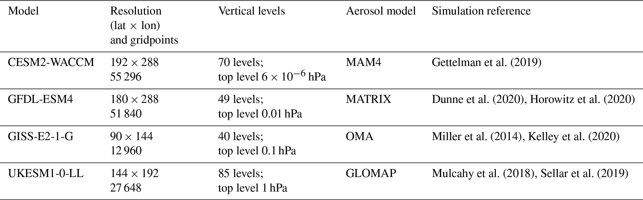
CESM2-WACCM (hereafter “CESM”) is a fully coupled Earth system model that integrates the Community Earth System Model version 2 (Emmons et al., 2020) with the Whole Atmosphere Community Climate Model version 6 (WACCM6). The atmospheric component operates at a horizontal resolution of 0.9375° latitude by 1.25° longitude, with 70 hybrid sigma-pressure vertical layers extending from the surface to $\mathrm{6}\times {\mathrm{10}}^{-\mathrm{6}}$ hPa. Its interactive chemistry and aerosol modules include the troposphere, stratosphere, and lower thermosphere, with a comprehensive treatment of 231 species, 150 photolysis reactions, 403 gas-phase reactions, 13 tropospheric heterogeneous reactions, and 17 stratospheric heterogeneous reactions (Emmons et al., 2020). The model utilizes the four-mode Modal Aerosol Model (MAM4) (Emmons et al., 2020) and features its secondary organic aerosol (SOA) framework based on the Volatility Basis Set (VBS, Donahue et al., 2013) approach. The photolytic calculations use both inline chemical modules and a lookup table approach, which does not consider changes in aerosols.

The Atmospheric Model version 4.1 (AM4.1, Horowitz et al., 2020) within the GFDL Earth system model (Dunne et al., 2020) incorporates an interactive chemistry scheme that spans both the troposphere and stratosphere (GFDL-ESM4; hereafter “GFDL”). The atmospheric component operates at a horizontal resolution of 1° latitude by 1.25° longitude, with 49 hybrid sigma-pressure vertical layers extending from the surface to 0.01 hPa. This scheme includes 56 prognostic tracers, 36 diagnostic species, 43 photolysis reactions, 190 gas-phase kinetic reactions, and 15 heterogeneous reactions. Stratospheric chemistry accounts for key O₃ depletion cycles (O_x, HO_x, NO_x, ClO_x, and BrO_x) and heterogeneous reactions on stratospheric aerosols (Austin et al., 2013). Photolysis rates are calculated dynamically with the FAST-JX version 7.1 code, which considers the radiative impacts of modeled aerosols and clouds. The chemical mechanism is further elaborated in Horowitz et al. (2020), and the gas-phase and heterogeneous chemistry are similar to those employed by Schnell et al. (2018). Non-interactive natural emissions of O₃ precursors are prescribed as outlined in Naik et al. (2013a).

The GISS model, developed by the NASA Goddard Institute for Space Studies, integrates the chemistry-climate model version E2.1 with the GISS Ocean v1 (G01) model (GISS-E2-1-G; hereafter “GISS”). The specific configurations of this model utilized for the CMIP6 are detailed in Kelley et al. (2020). In this study, we focus on the model subset that includes online interactive chemistry. The atmospheric component operates at a horizontal resolution of 2° latitude by 2.5° longitude, with 40 hybrid sigma-pressure vertical layers extending from the surface to 0.1 hPa. The interactive chemistry module employs the GISS Physical Understanding of Composition-Climate Interactions and Impacts (G-PUCCINI) mechanism for gas-phase chemistry (Kelley et al., 2020; Shindell et al., 2013). For aerosols, the model utilizes either the One-Moment Aerosol (OMA) or the Multiconfiguration Aerosol Tracker of Mixing state (MATRIX) model (Bauer et al., 2020). The gas-phase chemistry involves 146 reactions, including 28 photodissociation reactions, affecting 47 species across the troposphere and stratosphere, along with an additional five heterogeneous reactions. The model transports 26 aerosol particle tracers and 34 gas-phase tracers (OMA).

UKESM represents the United Kingdom's Earth system model (Sellar et al., 2019). It builds upon the Global Coupled 3.1 (GC3.1) configuration of HadGEM3 (Williams et al., 2018), incorporating additional Earth system components, such as ocean biogeochemistry, the terrestrial carbon-nitrogen cycle, and atmospheric chemistry (UKESM1-0-LL; hereafter “UKESM”). Walters et al. (2019) provided descriptions of the atmospheric and land components. The atmospheric component operates at a horizontal resolution of 1.25° latitude by 1.875° longitude, with 85 vertical layers extending from the surface to 85 km. The chemistry module in the UKESM model is a unified stratosphere-troposphere scheme (Archibald et al., 2020) including 84 tracers, 199 bimolecular reactions, 25 unimolecular and termolecular reactions, 59 photolytic reactions, 5 heterogeneous reactions, and 3 aqueous-phase reactions for the sulfur cycle from the United Kingdom Chemistry and Aerosols (UKCA) model. The aerosol module is based on the two-moment scheme from UKCA, known as GLOMAP mode, and is integrated into the Global Atmosphere 7.0/7.1 configuration of HadGEM3 (Walters et al., 2019). The UKESM uses interactive Fast-JX photolysis scheme, which is applied to derive photolysis rates between 177 and 850 nm, as described in Telford et al. (2013). In the lower mesosphere, photolysis rates are calculated using lookup tables (Lary and Pyle, 1991).

Models differ in their representation of O₃ source and sink processes, as well as in the definitions of the associated budget terms, which contributes to variability in model outcomes (Stevenson et al., 2006; Young et al., 2018). For example, in the GISS model, the tropospheric chemistry component simulates the NO_x-HO_x-O_x-CO-CH₄ system and the oxidation pathways for non-methane volatile organic compounds (NMVOCs). Central to these discrepancies are the treatments of non-methane volatile organic compound NMVOCs chemistry, which impacts both chemical production and destruction rates, along with surface removal mechanisms and stratospheric influences. Furthermore, the choice of tropopause definition can significantly alter the diagnosed O₃ burden, as well as the flux from the stratosphere.

All four of the interactive tropospheric chemistry models contain parameterizations of the nitrogen oxide (NO_x) emissions from lightning based on the height of the convective cloud top (Price et al., 1997; Price and Rind, 1992; Price, 2013), and the tropopause height for each model based on the WMO definition. Each model has a different way of implementing emissions and how much they are profiled. For instance, online calculations of lightning NO_x emissions during deep convection in the GISS model are based on the method described by Kelley et al. (2020). Lightning NO_x continues to be a major source of uncertainty in both model comparisons and the temporal development of tropospheric O₃ because it has a disproportionately significant influence on tropospheric-O₃ concentration relative to surface emissions (Murray et al., 2013).

BVOC emissions are modeled as a function of vegetation type and cover, as well as temperature and photosynthetic rates (gross primary productivity) (Unger, 2014; Sporre et al., 2019; Pacifico et al., 2011; Guenther et al., 1995). While models vary in the speciation of emitted VOCs, they commonly include isoprene and monoterpenes, each with its own distinct emission parameterization. Despite the common reliance on photosynthetically active radiation for the parameterization of BVOC emissions across the four models, there exist notable distinctions. For instance, the GFDL model exclusively considers the leaf area index, neglecting the impact of temperature on BVOC emissions, and the CESM, GISS, and UKESM models omit the influence of vegetation type from their calculations.

2.2 Simulation data and experimental design

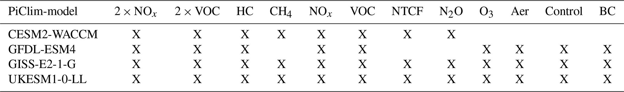
The primary objective of AerChemMIP is to quantitatively ascertain the influence of aerosols and reactive trace gases on the climate system, as well as the bidirectional feedback mechanisms involved (Collins et al., 2017). Table 2 presents a synopsis of the experimental configurations employed in this study. The control experiment, denoted as PiClim-control, is designed to stabilize both atmospheric composition and climatic conditions at a state reminiscent of the pre-industrial era, where the natural fractions of stratospheric ozone forcing species such as halocarbons was extremely low, specifically 1850 (radiative forcing contribution of ozone-depleting halocarbons approximately 0.12 W m⁻²) (Thornhill et al., 2021). The PiClim-2x experiment involves doubling of individual natural emission fluxes relative to the 1850 control, while the PiClim-x experiments calibrate these fluxes to align with the emission levels prevalent in 2014 (Collins et al., 2017). PiClim-2xNO_x represents to doubling of the nitric oxide emissions from natural sources due to lightning activity. PiClim-2xVOC represents to doubling of the volatile organic compound emissions from natural sources, including isoprene and monoterpenes. PiClim-HC represents the pre-industrial climatological control with 2014 halocarbons emissions both from anthropogenic (CFCs, HCFCs and compounds containing bromine) and natural sources. PiClim-CH₄ represents the pre-industrial climatological control with 2014 methane emissions both from anthropogenic and natural sources. PiClim-NO_x represents the pre-industrial climatological control with 2014 nitrogen oxide emissions both from anthropogenic and natural sources. PiClim-VOC represents the pre-industrial climatological control with 2014 VOC emissions both from anthropogenic and natural sources. PiClim-NTCF represents the pre-industrial climatological control with 2014 near-term climate forcers emissions, including aerosols and chemically reactive gases such as tropospheric ozone and methane. PiClim-N₂O represents the pre-industrial climatological control with 2014 nitrous oxide emissions both from anthropogenic and natural sources. PiClim-aer represents the pre-industrial climatological control with 2014 aerosol concentrations. PiClim-O₃ represents the pre-industrial climatological control with 2014 ozone concentrations. PiClim-BC represents the pre-industrial climatological control with 2014 black carbon concentrations.

Table 2 The available experiments of selected models in this study. “X” represents the experiment is available.

We analyzed models that had archived sufficient data in the Earth System Grid Federation (ESGF) system to permit accurate characterization of tropospheric O₃. In practice this meant we used archived O₃ data from the AERmon characterization of the tropospheric O₃ (variable name: “o3”) on native model grids. Other variables used include chemical production (variable name: “o3prod”), chemical destruction (variable name: “o3loss”), nitrogen monoxide (variable name: “no”), nitrogen dioxide (variable name: “no2”), isoprene (variable name: “isop”), organic dry aerosol (variable name: “emioa”), and secondary organic aerosol (variable name: “mmrsoa”). All data used in this paper are available on the Earth System Grid Federation website and can be downloaded from https://esgf-node.ipsl.upmc.fr/search/cmip6-ipsl/ (last access: 4 July 2024, ESGF-CEDA, 2024).

A new set of historical anthropogenic emissions has been developed with the Community Emissions Data System (CEDS, Hoesly et al., 2018). CEDS uses updated emission factors to provide monthly emissions of the major aerosol and trace gas species over the period 1750 to 2014 for use in CMIP6, and biomass burning emissions are based on a different inventory developed separate from CEDS (Van Marle et al., 2017). The primary analysis examines emissions of NO_x and VOCs from anthropogenic (Hoesly et al., 2018) and biomass burning sources (van Marle et al., 2017) that were provided as a common emission inventory to be used by all models (including the four in this study) in CMIP6 simulations. In the CESM and GFDL models, biogenic emissions, including isoprene and monoterpenes, are calculated interactively using MEGAN version 2.1 (Guenther et al., 2012) and are further utilized for SOA formation. While in the GISS model, biogenic emissions of isoprene are computed online and are sensitive to temperature (Shindell et al., 2006), whereas alkenes, paraffins, and terpenes are prescribed. And in the UKESM model, emissions of isoprene and monoterpenes are interactively calculated using the iBVOC emission model (Pacifico et al., 2011).

3 Results and discussions

3.1 Spatial, seasonal, and vertical distribution of tropospheric O₃

We first investigate the seasonal and vertical variations of ozone volume mixing ratio in the pre-industrial atmospheres simulated by four selected models. The analysis of tropospheric O₃ data derived from the PiClim experiment outcomes (five experiments common to the four models, including PiClim-2NO_x, PiClim-NO_x, PiClim-2VOC, PiClim-VOC, and PiClim-HC) of CMIP6 models reveals distinct seasonal cycles and inter-model variations (Fig. 1). The GISS model demonstrates the highest simulated tropospheric column O₃ volume mixing ratio at 50.29 ppbv in the 29th and 30th year of simulation, followed by the UKESM (44.50 ppbv), CESM (38.02 ppbv), and GFDL (31.03 ppbv), where the height of the tropopause is based on the definition of WMO. These are consistent with previous findings from historical experiments (Griffiths et al., 2021).

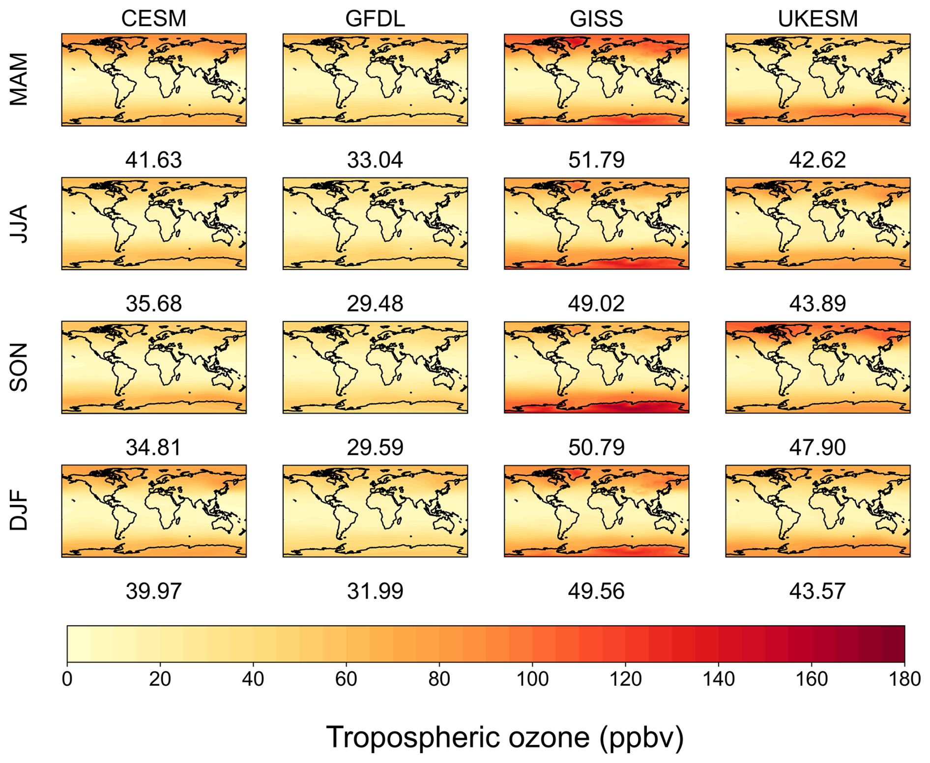
Figure 1 Comparison of the seasonal cycle of tropospheric column averaged volume mixing ratio of O₃ (density weighted) of the PiClim experiment results in the 29th and 30th year of simulation of the four models. Each row shows a separate meteorological season, arranged from top to bottom: March to May (MAM), June to August (JJA), September to November (SON), and December to February (DJF). Each column represents a selected model, listed from left to right: CESM, GFDL, GISS, and UKESM. The figures displayed below each chart represent the global tropospheric average ozone volume mixing ratio.

Furthermore, our analysis indicates that the disparity in O₃ volume mixing ratio during the PiClim experiment primarily occurs in polar regions. This may be attributed to the GISS model's ability to replicate a more robust entrainment of stratospheric O₃, a key source of tropospheric O₃ in the pre-industrial atmosphere, particularly at the poles. Previous studies have demonstrated that elevated O₃ levels in the Arctic during MAM and DJF, as well as in the Antarctic during JJA and SON, result from the cumulative impact of the polar O₃ barrier (Romanowsky et al., 2019).

Seasonal variations in tropospheric O₃ volume mixing ratio exhibit model-specific patterns. The CESM, GFDL, and GISS models simulate peak tropospheric O₃ volume mixing ratio in spring during the PiClim experiments. In contrast, the UKESM model reproduces maximum O₃ volume mixing ratio in autumn, indicating a limited capability in simulating dynamic circulations in the tropopause. Furthermore, the seasonal O₃ cycle simulations in CESM, GFDL, and GISS exhibit distinct discrepancies in their outcomes. For instance, the CESM model simulates the lowest O₃ volume mixing ratio in SON, while the GFDL model exhibits the lowest volume mixing ratio in JJA. The GISS model simulation indicates higher O₃ levels in autumn compared to DJF, which is consistent with results from historical experiments (Griffiths et al., 2021). Additionally, our analysis reveals that the CESM simulations demonstrate the most pronounced seasonal oscillation amplitude in O₃ volume mixing ratio, approximately 6.82 ppbv. This feature underscores the model's sensitivity to seasonal factors affecting tropospheric O₃ dynamics.

In the PiClim experiments, all four models accurately reproduce the peak volume mixing ratio of O₃ in the middle stratosphere at 10 hPa and the zonal average mixing ratios reaching their peak in the upper troposphere, particularly in extratropical regions, indicative of extended chemical lifetimes at higher altitudes. However, notable disparities are observed in the vertical distribution characteristics of O₃ among the four models (Fig. 2). Specifically, the CESM model exhibits the highest vertical extension, including an additional hotspot simulated in the thermosphere. While the GFDL and CESM2 models exhibit consistent simulation outcomes below 0.01 hPa, GISS and UKESM simulate significantly higher stratospheric O₃ levels at 10 hPa in comparison.

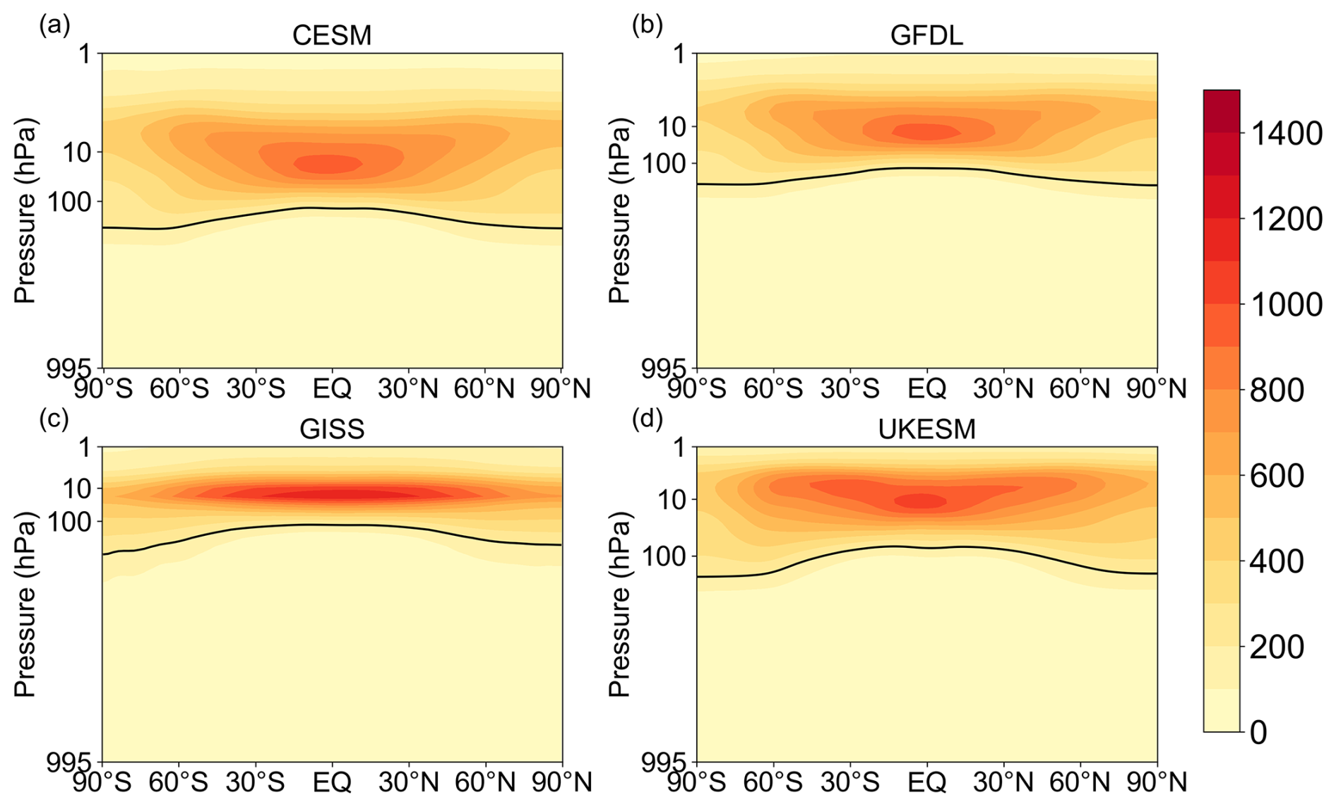
Figure 2 The zonal mean O₃ distribution for the 29th and 30th year of the PiClim experiment results from the (a) CESM, (b) GFDL, (c) GISS, and (d) UKESM model. Thick black lines represent the tropopause height for each model based on the WMO definition. Note: Each model is displayed on its native vertical pressure levels to preserve data integrity without interpolation, as applies for all related figures thereafter.

Notable distinctions are observed in the spatial distribution of O₃. The GISS model simulates a more vertically concentrated and latitudinally extended O₃ distribution. This characteristic may be a crucial factor contributing to the pronounced impact of O₃ transport in the polar stratosphere, as simulated by GISS. The zonal variability in O₃ distribution simulated by the UKESM falls between that of the GISS and CESM models. These inter-model discrepancies in O₃ simulation results likely reflect suboptimal representation of local and regional dynamics, as well as omitted chemical processes in corresponding models. The variability and uncertainty in O₃ precursor emission estimates further exacerbate these disparities.

Table 3 The averaged volume mixing ratio of global stratospheric ozone at all simulated vertical levels in the 29th and 30th year for each experiment of four models (ppbv).

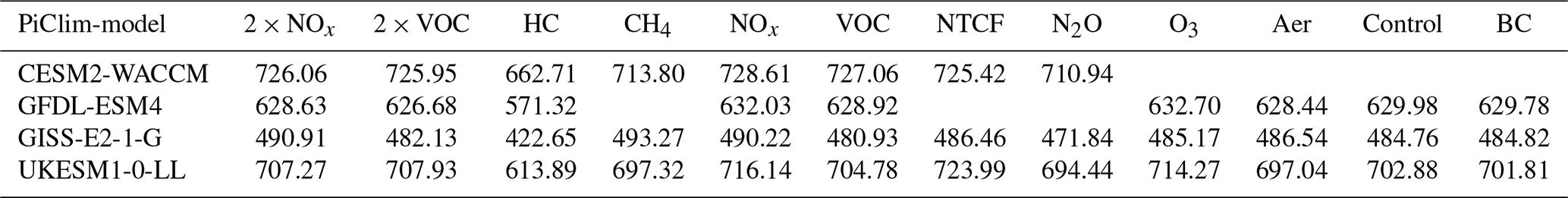
Table 4 The averaged volume mixing ratio of global tropospheric ozone in the 29th and 30th year for each experiment of four models (ppbv).

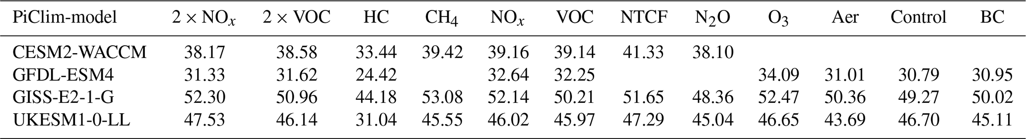
3.2 Characteristics of stratospheric and tropospheric O₃ of various experiments

Tables 3 and 4 present the stratospheric O₃ volume mixing ratio and tropospheric O₃ volume mixing ratio across all experiments from the four different models. The GISS model simulations show higher tropospheric O₃ volume mixing ratios, reflecting increased rates of stratospheric downwelling and surface O₃ precursor emissions. However, its overall O₃ volume mixing ratio is notably lower compared to the UKESM, CESM, and GFDL models, with reductions of 114.24, 76.16, and 47.04 ppbv, respectively. Analysis reveals that in the CESM, GFDL, and GISS models, the global O₃ molar fraction in the PiClim-2NO_x and PiClim-NO_x experiments surpasses that in the PiClim-2VOC and PiClim-VOC experiments. This difference is most pronounced in the GISS model, aligning with previous findings indicating its heightened sensitivity to NO_x response (Turnock et al., 2019). Conversely, in the UKESM model, the global O₃ molar fraction of the PiClim-2NO_x experiment is lower than that of the PiClim-2VOC experiment. Interestingly, the tropospheric O₃ volume mixing ratios in the PiClim-2NO_x experiment in the CESM and GFDL models are notably lower than in their respective PiClim-2VOC experiments, with reductions of 0.41 and 0.29 ppbv. This discrepancy challenges the conventional understanding that increased NO_x emissions from lightning activity should lead to tropospheric O₃ generation, suggesting a need for enhanced sensitivity simulations in these two models regarding O₃ and NO_x emissions from natural sources due to lightning activity. In contrast, the PiClim-2NO_x experiments of the GISS and UKESM models effectively simulate an increase in tropospheric O₃ volume mixing ratio compared to their PiClim-2VOC experiments. Furthermore, across all four models, the tropospheric O₃ volume mixing ratio of the PiClim-NO_x experiment surpasses that of the PiClim-VOC experiment, indicating the models' ability to accurately replicate the impact of rising anthropogenic emissions on O₃ production. Additionally, methane, a crucial natural source of volatile organic compounds and a key greenhouse gas, enhances tropospheric O₃ generation by CH₄ oxidation and influencing temperature, thereby elevating global O₃ volume mixing ratio. This phenomenon contributes to the heightened sensitivity of O₃ to methane volume mixing ratio in a clean atmosphere. Elevated volume mixing ratios of HCFCs (PiClim-HC) and nitrous oxide (PiClim-N₂O) lead to substantial stratospheric O₃ depletion, consequently affecting tropospheric O₃ volume mixing ratio through the pod coil process. Other influencing factors, such as aerosols and black carbon, induce warming through radiation effects, thereby simulating elevated O₃ volume mixing ratio.

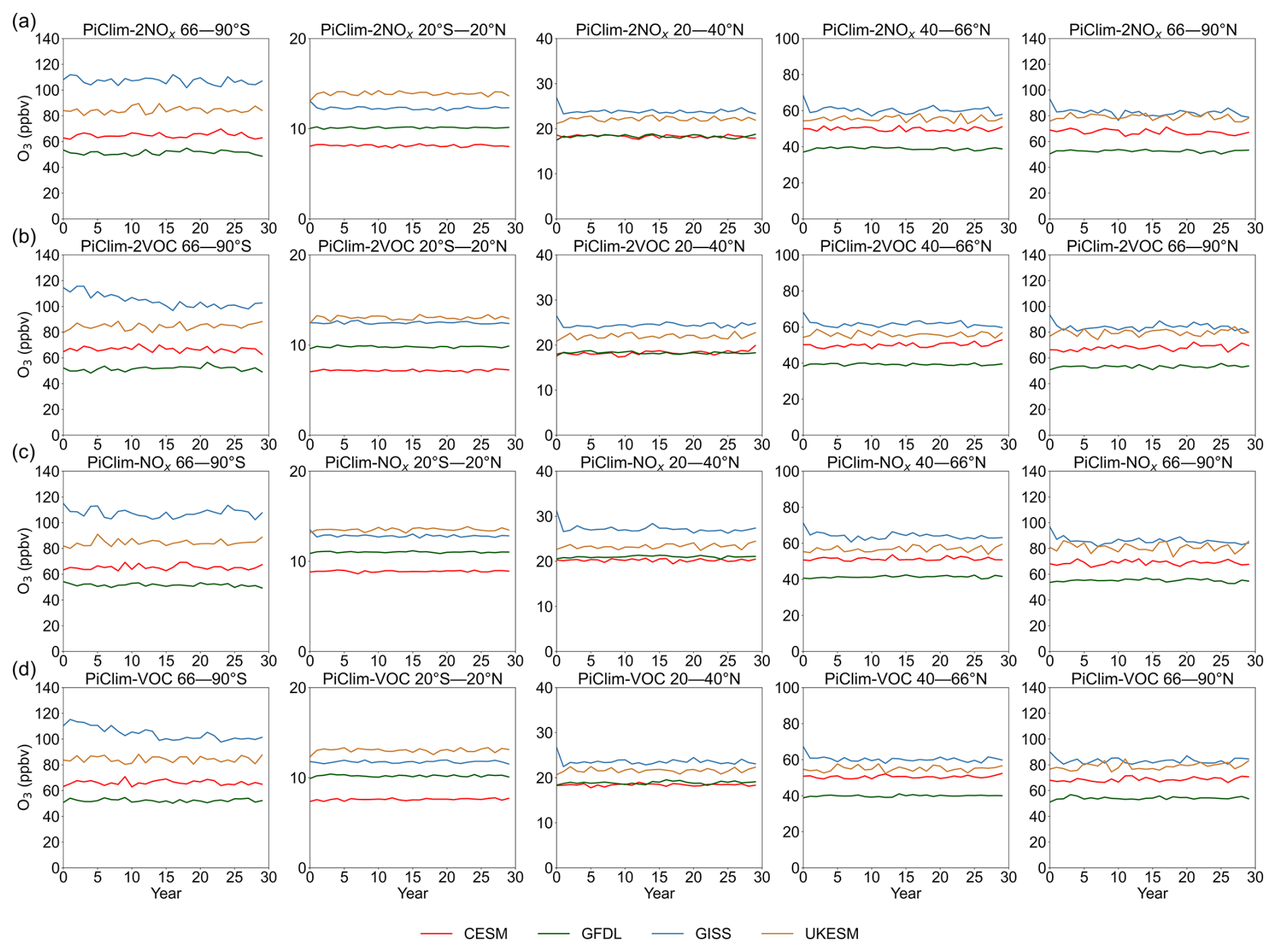
Figure 3 The temporal evolution characteristics of annual mean tropospheric column averaged O₃ volume mixing ratio at different latitudes for each model are presented for the (a) PiClim-2NO_x, (b) PiClim-2VOC, (c) PiClim-NO_x, and (d) PiClim-VOC experiment, the 4 models are represented by different line colors.

Figure 3 shows the temporal evolution of tropospheric O₃ levels across various latitudes, as simulated by four distinct models in O₃ precursor experiments. In the PiClim experiments, none of the models predicted an enhancement in O₃ volume mixing ratio with simulation time at all latitudes, reflecting the consistent chemical lifetime of O₃ within the pristine atmospheric conditions. However, discrepancies in O₃ predictions among the models become more pronounced with increasing latitudes. While the CESM model generally exhibits higher tropospheric O₃ volume mixing ratios compared to the GFDL model, it paradoxically portrays the lowest O₃ levels in the equatorial region. The GISS model demonstrates a marked disparity in tropospheric O₃ volume mixing ratios between the Antarctic and Arctic regions, with the former registering notably higher levels. In contrast, the CESM and GFDL models exhibit similar patterns in this regard. A unique feature of the GISS model is a notable declining trend in Antarctic tropospheric O₃ levels during the initial 15 years of both the PiClim-2VOC and PiClim-VOC experiments. This trend is not observed in the CESM, GFDL, and UKESM models, highlighting the sensitivity of the GISS model to precursors in simulating ozone is still higher than that of other models even in the pre-industrial clean atmosphere. The same conclusion was reached for NO_x experiments, but the ozone forcing was less than that in the VOC experiments. The UKESM model stands out with its pronounced simulation of elevated O₃ volume mixing ratios in the tropical belt. Furthermore, the PiClim-2xVOC experiment conducted within the UKESM model demonstrates a significant O₃ response to enhanced emissions of VOCs from natural sources in the equatorial region. This suggests a strong sensitivity of O₃ in the UKESM to increases in VOC emissions from natural sources.

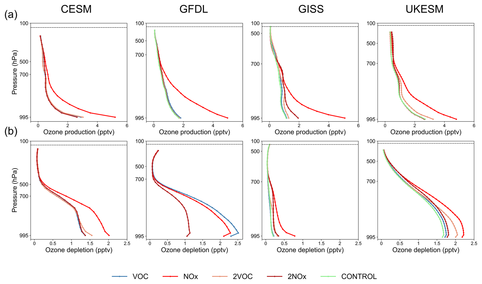
Figure 4 Vertical profiles of O₃ volume mixing ratio (a) chemical production and (b) chemical depletion rate for the 30th year across five experiments (it should be noted that the PiClim-control experiment data of the CESM model is not available) in the four models.

3.3 Analysis of O₃ generation in precursor experiments

In the shown subset of PiClim experiments, the O₃ production was defined as the cumulative tendency from HO₂, CH₃O₂, RO₂, and NO reactions, while O₃ loss encompassed the sum of O(1D)+H₂O, O₃+HO₂, OH+O₃, and O₃+alkene reactions. Figure 4 depicts the chemical production and consumption of tropospheric ozone in the five simulations performed by the four models. The GISS demonstrates the lowest O₃ chemical production among the models, whereas the other three models show generally consistent production levels. Notably, the GISS model exhibits a relatively low efficiency in O₃ chemical consumptions, primarily due to missing the loss of O₃ with isoprene and terpenes process. The low offset of ozone production and depletion in the pre-industrial atmosphere by the GISS model provides a new perspective based on previous studies indicating the high offset of ozone production and depletion in the present atmosphere by the GISS model. The four models all showed high ozone chemical production in the PiClim-NO_x experiment, indicating that the four all have perfect ability to simulate the photochemical generation mechanism of tropospheric ozone. However, the CESM and GFDL models do not show a significant increase in tropospheric O₃ chemical generation during the PiClim-2NO_x experiment. And although the GISS and UKESM models successfully simulated an increase in the O₃ chemical generation rate due to heightened lightning activity in this experiment, these increases in ozone production are also much smaller than the chemical production generated by the PiClim-NO_x experiment, which might show that the theoretical mechanism of ozone sensitivity to natural precursors in pre-industrial atmosphere differs from the present mechanism due to the differences in the characteristics of intermediate products such as OH. Furthermore, in either model, the ozone chemical production from the PiClim-NO_x experiment, while higher than in other experiments other than PiClim-NTCF, is much smaller than the ozone chemical production caused by this emission inventory in the atmosphere today (Fig. S5). Today's NO_x emission forcing has not led to a sustained increase in the ozone volume mixing ratio in the pre-industrial atmosphere over a long-time scale, which indicates important differences between the pre-industrial atmosphere and the present atmosphere in terms of the ozone generation environment and the ozone depletion environment.

Furthermore, the PiClim-2VOC experiment in the CESM and GFDL models lead to an increase in tropospheric O₃ volume mixing ratio, despite not reproducing higher O₃ chemical production. The UKESM model successfully captures the enhancement of O₃ chemical formation due to increased emissions of VOCs from natural sources, underscoring its precise sensitivity to these emissions and validating its capability to simulate O₃ dynamics influenced by them. However, the global O₃ volume mixing ratio in the PiClim-2xVOC experiment of these models is lower than that of the PiClim-VOC experiment. These observations illustrate the variability among models in capturing the O₃ response to its precursor species, stemming from varied treatments of critical atmospheric processes, including photolysis, dry deposition, transport mechanisms, and mixing dynamics. Furthermore, these findings highlight the variability in global O₃ sensitivity compared to local O₃ sensitivity, underscoring the complexity of studying O₃ sensitivity on a global scale to mitigate its climate impacts.

Figure 4b illustrates that, apart from the O₃ chemical formation mechanism, the CESM, GFDL, and UKESM models in the PiClim-2NO_x experiment do not accurately depict the O₃ chemical depletion process induced by NO_x. Despite successfully replicating the rise in NO and NO₂ levels (Fig. 5a and b) in the upper troposphere, these models fall short in capturing the NO_x-related O₃ depletion phenomenon. Moreover, the GISS model stands out with notably elevated NO_x volume mixing ratios attributed to heightened lightning activity compared to the other models. Additionally, it demonstrates a peak NO_x volume mixing ratio near 500 hPa across these five experiments conducted, a feature not observed in the other models.

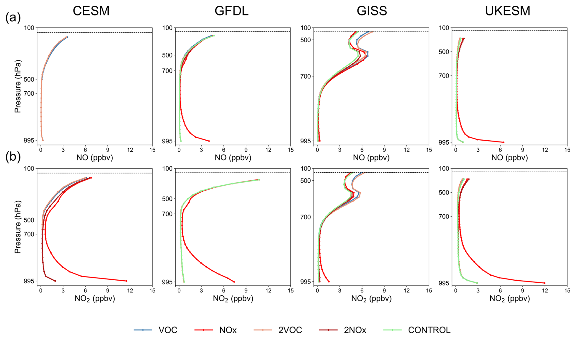
Figure 5 Vertical profiles of (a) NO and (b) NO₂ volume mixing ratios for the 30th year across five experiments in the four models. Note that the PiClim-control experiment data of the CESM model is not available.

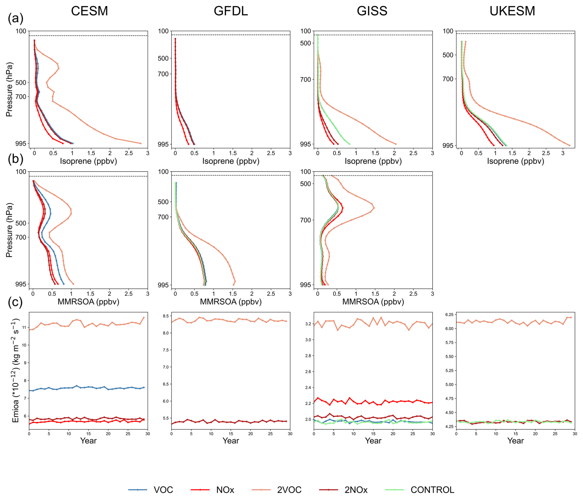
Figure 6 Vertical profiles of (a) isoprene volume mixing ratio and (b) secondary organic aerosol mass mixing ratio for the 30th year of all available experiments across the three models. (c) Temporal evolution characteristics of major emissions and the chemical production of organic dry aerosol particles from five experiments of the four models. Note that the PiClim-control experiment data of the CESM model is not available.

Figure 6 illustrates a notable inverse correlation between the consumption of isoprene and the chemical production of O₃ in four models, when the rise in VOCs emissions is not factored in. This relationship is attributed to the significance of isoprene as a natural VOC source in unpolluted atmospheres and highlights the absence of O₃ generation simulation due to lightning activity in the CESM, GFDL, and UKESM models. In the PiClim experiments, the UKESM model did not provide mass fraction of secondary particulate organic matter dry aerosol particles in the air (mmrsoa), and so we only include its volume mixing ratio of isoprene in the air (isop) and the primary emissions and chemical production of dry aerosol organic matter (emioa) in Fig. 6. Additionally, the CESM model exhibits higher emissions and chemical formation of organic dry aerosol particles compared to the GFDL and GISS models. This difference potentially contributes to the observed variation in global O₃ volume mixing ratios, with the highest levels recorded in the CESM model and the lowest in the GISS model. The vertical variation characteristics of ozone chemical production, chemical consumption, nitrogen oxides, and VOCs in the other seven experiments of the four models are characterized in the Supplement (Figs. S5–S7).

4 Conclusions

This study assessed the sensitivity of global-scale ozone (O₃) to precursor gases in a clean atmosphere and evaluated the simulation capabilities of four Earth system models using data from the PiClim experiments within the AerChemMIP framework. Our results highlight both strengths and limitations of these models in capturing O₃ response. The CESM and GFDL models excelled in reproducing seasonal O₃ cycles and the vertical distribution of O₃, but they showed limitations in simulating the tropospheric O₃ response to NO_x emissions from natural sources, such as lightning activity. Conversely, the GISS and UKESM models effectively simulated the positive correlation between tropospheric O₃ and temperature but were less sensitive to natural precursors compared to anthropogenic sources. Discrepancies, such as zonal temperature biases in the GISS model and stratospheric temperature inconsistencies in the GFDL model, underscore areas for improvement.

Our findings suggest that existing assumptions regarding O₃ sensitivity to natural precursors may require refinement in clean atmospheric conditions. This research provides critical insights into the interplay between O₃ and its precursors, enhancing the accuracy of O₃ simulations in Earth system models. Given the significant role of O₃ in radiative forcing, atmospheric oxidation, and climate feedback mechanisms, our study reinforces the necessity of precise modeling to better predict and mitigate future climate scenarios. Additionally, the results underscore the importance of controlling anthropogenic precursor emissions as an essential strategy to manage tropospheric O₃ volume mixing ratios and address broader climate change challenges. Furthermore, among the models analyzed, only the GISS model demonstrates a significant increase in Antarctic ozone levels compared to the Arctic (Fig. 3); the other three models yield similar ozone concentrations at both polar regions. This discrepancy seems to result from a distinct characteristic of the GISS model's dynamical representation of the Antarctic polar vortex. Figure 1 also reveals that the ozone difference in the GISS model is predominantly confined to JJA and SON (Antarctic winter-spring).

It is important to acknowledge that the results generated by the models are accompanied by a degree of uncertainty. Variations in the methodologies employed by different models to address chemical reactions, including the production and depletion of ozone, contribute to the uncertainty surrounding the ozone budget. Furthermore, discrepancies in the data pertaining to anthropogenic and natural emissions, particularly concerning NO_x and BVOC emissions, substantially influence the outcomes of these models. Additionally, the uncertainty associated with the stratosphere-troposphere exchange process represents a critical factor in the ozone budget, with notable divergences in the treatment of this process across various models.