Advances in CALIPSO (IIR) cirrus cloud property retrievals – Part 1: Methods and testing

In this study, we describe an improved Cloud-Aerosol Lidar and Infrared Pathfinder Satellite Observation (CALIPSO) satellite retrieval which uses the CALIPSO Imaging Infrared Radiometer (IIR) and the CALIPSO lidar for retrievals of ice particle number concentration N_i, effective diameter D_e and ice water content (IWC). By exploiting two IIR channels, this approach is fundamentally different from another satellite retrieval based on cloud radar and lidar that retrieves all three properties. A global retrieval scheme was developed using in situ observations from several field campaigns. The N_i retrieval is formulated in terms of $N_{\mathrm{i}}/A_{\mathrm{PSD}}$ ratios, where A_PSD is the directly measured area concentration of the ice particle size distribution (PSD), along with the absorption optical depth in two IIR channels and the equivalent cloud thickness seen by IIR. It is sensitive to the shape of the PSD, which is accounted for, and uses a more accurate mass-dimension relationship relative to earlier work. The new retrieval is tested against corresponding cloud properties from the field campaigns used to develop this retrieval, as well as a recent cirrus cloud property climatology based on numerous field campaigns from around the world. In all cases, favorable agreement was found. This analysis indicated that N_i varies as a function of τ. By providing near closure to the ice PSD, the natural atmosphere may be used more like a laboratory for studying key processes responsible for the evolution and life cycle of cirrus clouds and their impact on climate.

1 Introduction

Cirrus clouds contain only ice particles (i.e., no liquid cloud droplets), a condition guaranteed when cloud temperatures (T) are less than $\sim -$38 °C (Koop et al., 2000). The microphysical and radiative properties of cirrus clouds are subject to very different ice nucleation pathways as well as whether the cirrus clouds are of liquid origin or not (e.g., Krämer et al., 2016), and they also depend on aerosol particles of different sizes in complex ways (Ngo et al., 2024). With the ice particle size distribution (PSD) of cirrus clouds subject to so many factors, factors that may vary with latitude, season and surface type (e.g., land vs. ocean), there is a need to observe cirrus cloud PSDs from space if cirrus clouds are to be represented accurately in climate models. If PSDs in cirrus clouds are approximated as exponential, they can be characterized through satellite retrievals of the PSD ice water content (IWC), effective diameter (D_e) and ice particle number concentration (N_i) as described in Mitchell et al. (2020). Such satellite retrievals appear to be a necessary but not sufficient condition for understanding aerosol-cloud-climate interactions in cirrus clouds.

Ice crystals in cirrus clouds can form by either of two processes: homogeneous or heterogeneous ice nucleation (henceforth hom and het). The former requires no ice nucleating particles and can proceed through the freezing of haze and cloud solution droplets when T≤235 K (−38 °C) and the relative humidity with respect to ice (RH_i) exceeds some threshold where RH_i > ∼ 145 % (Koop et al., 2000). This results in generally higher concentrations of ice particles (N_i) relative to het (Barahona and Nenes, 2009; Jensen et al., 2012, 2013a, b; Cziczo et al., 2013). Under weak updraft conditions, N_i resulting from hom may be similar to N_i resulting from het (Krämer et al., 2016), and under atypical conditions (such as high concentrations of mineral dust), N_i resulting from het can exceed 200 L⁻¹ which is characteristic of hom (Barahona and Nenes, 2009; Cziczo et al., 2013). In cirrus clouds, het may occur at any RH_i > 100 %, and in the context of a cloud parcel moving in an updraft, ice is first produced through het, and subsequently through hom if the het-produced ice crystals do not prevent the RH_i from reaching the threshold RH_i needed for hom to occur (e.g., Haag et al., 2003). Overall, cirrus clouds formed primarily through hom will probably have substantially higher N_i and IWC (due to the higher RH_i of ice formation) relative to cirrus formed primarily through het (Krämer et al., 2016). Since the cirrus cloud extinction coefficient for sunlight is proportional to IWC $/D_{\mathrm{e}}$, these two types of cirrus clouds (i.e., hom and het dominated cirrus) may therefore display considerably different radiative properties.

In addition to extinction effects, relatively high N_i produced through hom can result in smaller ice crystals that fall slower relative to het-formed ice crystals (Krämer et al., 2016). These lower ice fall speeds contribute to higher IWCs and longer cloud lifetimes, and thus greater cloud coverage (Mitchell et al., 2008). In this way hom alters cloud radiative properties through changes in D_e and IWC (that affect cloud extinction and visible optical depth τ) and also cloud coverage. Many modeling studies have demonstrated the important impact that changes in ice fall speed have on climate (e.g., Sanderson et al., 2008; Mitchell et al., 2008; Eidhammer et al., 2017).

To date, there are two methods for retrieving all three cirrus cloud properties (N_i, D_e, IWC) from space: (1) the DARDAR approach based on the CloudSat Cloud Profiling Radar (CPR) and the Cloud-Aerosol Lidar and Infrared Pathfinder Satellite Observation (CALIPSO) lidar (i.e., Cloud and Aerosol Lidar with Orthogonal Polarization, or CALIOP), as described in Sourdeval et al. (2018) and Delanoë and Hogan (2010), and (2) a CALIPSO approach combining the CALIPSO Infrared Imaging Radiometer (IIR) with the CALIOP lidar, as described in Mitchell et al. (2018; henceforth M2018). These two approaches differ in many respects, with the DARDAR approach sensing optically thicker clouds due to the CPR (i.e., the CALIPSO approach is limited to visible cloud optical depths τ < ∼ 3). But 79 % of all ice clouds (of which cirrus clouds are a subcategory) have a τ < 3 (Hong and Liu, 2015). Moreover, the DARDAR N_i approach presumes a fixed PSD shape based on Delanoë et al. (2014) whereas the CALIPSO approach does not assume a PSD shape, but rather is based on PSD properties obtained from aircraft measurement probes during cirrus cloud field campaigns. Both methods are sensitive to small ice crystals (that dominate N_i) due to the lidar regarding (1) and due to photon tunneling (i.e., wave resonance) absorption regarding (2) which is most active when ice crystal lengths are comparable to the wavelength (∼ 10 µm in this case) as described in M2018.

This study presents a new CALIPSO satellite retrieval that borrows some methodology from M2018 but also develops new methods that greatly increase the sampling range of cirrus clouds and increase the accuracy of the retrievals. It is similar to M2018 in that it retrieves D_e, N_i and IWC by employing the effective absorption optical depth ratio, β_eff (a standard, well characterized CALIPSO IIR retrieval using retrieved absorption optical depths at 12.05 and 10.6 µm in this case), but it differs in that new equations are used for calculating N_i, D_e and IWC for greater accuracy and theoretical soundness as described in Sect. 2. As with M2018, empirical X–β_eff relationships are developed from cirrus cloud field campaigns as described in Sect. 3, where X is a microphysical property such as $N_{\mathrm{i}}/$ IWC, but IWC is estimated more accurately and the retrieval is based on more field campaigns. Moreover, retrievals (and ice cloud radiative properties) at terrestrial wavelengths can be sensitive to the shape of the PSD as described in Mitchell (2002) and Mitchell et al. (2011). Such a sensitivity was found in the case of tropical tropopause layer (TTL) cirrus clouds, where their PSD shape differed from the anvil cirrus clouds sampled at higher temperatures. Due to this PSD shape difference, TTL and anvil cirrus having the same β_eff can have different D_e, which was accounted for in this retrieval scheme. Finally, β_eff was obtained with the most recent CALIPSO Version 4.51 Level 2 products. In Sect. 4, the retrievals are tested against corresponding cloud properties from the field campaigns used to develop this method, as well as the cirrus cloud property climatology of Krämer et al. (2020) based on numerous cirrus cloud field campaigns. Conclusions are given in Sect. 5. Scientific discoveries resulting from this CALIPSO retrieval are described in Part 2 of this study (Mitchell and Garnier, 2025).

2 Developing a new CALIPSO IIR retrieval for cirrus cloud properties

2.1 Analytical formulation

The retrieval of M2018 is based on co-located observations from the IIR and the CALIOP lidar aboard the CALIPSO polar orbiting satellite. It retrieves N_i, D_e and IWC as a function of the effective absorption optical depth ratio β_eff, where β_eff=τ_abs (12.05 µm) $/$ τ_abs (10.6 µm) and τ_abs (12.05 µm) and τ_abs (10.6 µm) are the effective absorption optical depths retrieved in these IIR channels; β_eff is considered an effective ratio since the retrieval of β_eff from the cloud emissivity at each wavelength includes the effects of scattering. The N_i retrieval depends on three empirical β_eff relationships with D_e, the $N_{\mathrm{i}}/$ IWC ratio, and the PSD effective absorption efficiency at 12 µm Q_abs,eff (12 µm). These three β_eff relationships were derived from in situ measurements during cirrus cloud aircraft field campaigns. The latter is used to derive the visible layer extinction, α_ext, from τ_abs (12.05 µm) and the IIR equivalent cloud thickness Δz_eq. Layer N_i is derived from the $N_{\mathrm{i}}/$ IWC ratio after retrieving layer IWC from α_ext and the empirical D_e–β_eff relationship. The uncertainty in N_i can be reduced by eliminating its dependence on the empirical D_e–β_eff relationship and by replacing the $N_{\mathrm{i}}/$ IWC ratio with the $N_{\mathrm{i}}/A_{\mathrm{PSD}}$ ratio, where A_PSD is the PSD projected area per unit volume directly measured by the 2D-S probe (Lawson et al., 2006; Lawson, 2011). That is, the IWCs used to formulate the retrievals in M2018 were calculated from the ice particle projected area (A_p; directly measured by the 2D-S probe) and the ice particle mass (m)–A_p power law relationship of Baker and Lawson (2006), where considerable uncertainty in IWC enters through this m–A_p power law. This uncertainty can be eliminated by using the relationship between $N_{\mathrm{i}}/A_{\mathrm{PSD}}$ and β_eff, which can be determined from PSD in situ measurements during cirrus cloud field campaigns, analogous to the calculation of the $N_{\mathrm{i}}/$ IWC ratio as described in M2018.

To remove these uncertainties, the retrieval of M2018 was reformulated as follows. We begin by equating two different expressions for the effective absorption coefficient α_abs for a homogeneous single-layer cirrus cloud:

$$\begin{array}{}\text{(1)}& {\displaystyle \frac{{\mathit{\tau }}_{\mathrm{abs}}\left(\mathit{\lambda }\right)}{\mathrm{\Delta }{z}_{\mathrm{eq}}}}={\left[Q_{\mathrm{abs},\mathrm{eff}}\left(\mathit{\lambda }\right)\right]}_{{\mathit{\beta }}_{\mathrm{eff}}}{\left[{\displaystyle \frac{A_{\mathrm{PSD}}}{N_{\mathrm{i}}}}\right]}_{{\mathit{\beta }}_{\mathrm{eff}}}{N}_{\mathrm{i}},\end{array}$$

where τ_abs(λ) is the effective absorption optical depth at a given wavelength (λ), Q_abs,eff(λ) is the PSD effective absorption efficiency (${\mathit{\alpha }}_{\mathrm{abs}}/A_{\mathrm{PSD}}$) at the given wavelength and both Q_abs,eff and $A_{\mathrm{PSD}}/N_{\mathrm{i}}$ are empirical functions of β_eff (and are denoted accordingly). Moreover, A_PSD is an area concentration, having units of area per unit volume, while N_i is number per unit volume. This gives $A_{\mathrm{PSD}}/N_{\mathrm{i}}$ units of area per ice particle (e.g., cm²). Solving for N_i, and applying to the IIR channel at λ= 12.05 µm,

$$\begin{array}{}\text{(2)}& N_{\mathrm{i}}={\left[{\displaystyle \frac{N_{\mathrm{i}}}{A_{\mathrm{PSD}}}}\right]}_{{\mathit{\beta }}_{\mathrm{eff}}}{\displaystyle \frac{{\mathit{\tau }}_{\mathrm{abs}}\left(\mathrm{12.05}\mathrm{\mu }\mathrm{m}\right)}{{\left[Q_{\mathrm{abs},\mathrm{eff}}\left(\mathrm{12}\mathrm{\mu }\mathrm{m}\right)\right]}_{{\mathit{\beta }}_{\mathrm{eff}}}\mathrm{\Delta }{z}_{\mathrm{eq}}}}.\end{array}$$

Evaluating units, the right-hand side has units of reciprocal volume. As in M2018, β_eff and Q_abs,eff (12 µm) are based on in situ PSD measurements and the modified anomalous diffraction approximation (MADA) (Mitchell, 2000, 2002; Mitchell et al., 2006). Equation (2) is sensitive to the smallest ice crystals (which contribute the most to N_i) due to its dependence on β_eff, where β_eff is sensitive to photon tunneling (i.e., wave resonance) absorption, and this type of absorption is strongest when the ice particle size is comparable to the absorbed wavelength (e.g., M2018). The quantity Δz_eq is smaller than Δz, the cloud layer geometrical thickness measured by CALIOP, and accounts for the fact that the IIR instrument does not equally sense all levels of the cloud layer that contribute to thermal emission. This is accounted for through the IIR weighting profile as discussed in M2018 and Garnier et al. (2021a) and detailed later in Sect. 2.2.5.

The concept and definition of effective diameter D_e is given in Mitchell (2002) as

$$\begin{array}{}\text{(3)}& D_{\mathrm{e}}={\displaystyle \frac{\mathrm{3}\mathrm{IWC}}{\mathrm{2}{\mathit{\rho }}_{\mathrm{i}}{A}_{\mathrm{PSD}}}},\end{array}$$

where ρ_i is the bulk density of ice. This definition can be expanded to incorporate the β_eff relationships pertaining to $N_{\mathrm{i}}/A_{\mathrm{PSD}}$ and IWC $/N_{\mathrm{i}}$ (so that the N_i terms cancel):

$$\begin{array}{}\text{(4)}& D_{\mathrm{e}}={\displaystyle \frac{\mathrm{3}}{\mathrm{2}{\mathit{\rho }}_{\mathrm{i}}}}{\left[{\displaystyle \frac{N_{\mathrm{i}}}{A_{\mathrm{PSD}}}}\right]}_{{\mathit{\beta }}_{\mathrm{eff}}}{\left[{\displaystyle \frac{\mathrm{IWC}}{N_{\mathrm{i}}}}\right]}_{{\mathit{\beta }}_{\mathrm{eff}}},\end{array}$$

where the subscript β_eff indicates that these ratios are retrieved quantities related to β_eff. Since the D_e–β_eff relationship in M2018 was not as “tight” or precise as the $N_{\mathrm{i}}/$ IWC–β_eff relationship, and the $N_{\mathrm{i}}/A_{\mathrm{PSD}}$–β_eff relationship has a similar shape as the $N_{\mathrm{i}}/$ IWC–β_eff relationship, Eq. (4) is expected to reduce uncertainties in the retrieval of D_e.

Cirrus cloud climatologies such as those reported by Krämer et al. (2020) provide the spherical volume radius, R_v, of the mean ice particle mass, IWC $/N_{\mathrm{i}}$. Unlike D_e, R_v depends only on IWC $/N_{\mathrm{i}}$ as

$$\begin{array}{}\text{(5)}& R_{\mathrm{v}}={\left({\displaystyle \frac{\mathrm{3}}{\mathrm{4}\mathit{\pi }{\mathit{\rho }}_{\mathrm{i}}}}\right)}^{\mathrm{1}/\mathrm{3}}{\left[{\displaystyle \frac{\mathrm{IWC}}{N_{\mathrm{i}}}}\right]}_{{\mathit{\beta }}_{\mathrm{eff}}}^{\mathrm{1}/\mathrm{3}}.\end{array}$$

With unique retrieval equations for N_i and D_e, IWC is determined as

$$\begin{array}{}\text{(6)}& \mathrm{IWC}={\displaystyle \frac{{\mathit{\rho }}_{\mathrm{i}}}{\mathrm{3}}}{\mathit{\alpha }}_{\mathrm{ext}}{D}_{\mathrm{e}},\end{array}$$

where α_ext is the shortwave or visible extinction coefficient given as

$$\begin{array}{}\text{(7)}& {\mathit{\alpha }}_{\mathrm{ext}}=\mathrm{2}{\left[{\displaystyle \frac{\mathrm{1}}{Q_{\mathrm{abs},\mathrm{eff}}\left(\mathrm{12}\mathrm{\mu }\mathrm{m}\right)}}\right]}_{{\mathit{\beta }}_{\mathrm{eff}}}{\displaystyle \frac{{\mathit{\tau }}_{\mathrm{abs}}\left(\mathrm{12.05}\mathrm{\mu }\mathrm{m}\right)}{\mathrm{\Delta }{z}_{\mathrm{eq}}}}.\end{array}$$

Similarly, the cloud visible optical depth is given as

$$\begin{array}{}\text{(8)}& \mathit{\tau }=\mathrm{2}{\left[{\displaystyle \frac{\mathrm{1}}{Q_{\mathrm{abs},\mathrm{eff}}\left(\mathrm{12}\mathrm{\mu }\mathrm{m}\right)}}\right]}_{{\mathit{\beta }}_{\mathrm{eff}}}{\mathit{\tau }}_{\mathrm{abs}}\left(\mathrm{12.05}\mathrm{\mu }\mathrm{m}\right),\end{array}$$

and the cloud ice water path, IWP, is given as

$$\begin{array}{}\text{(9)}& \mathrm{IWP}={\displaystyle \frac{{\mathit{\rho }}_{\mathrm{i}}}{\mathrm{3}}}\mathit{\tau }{D}_{\mathrm{e}}.\end{array}$$

As noted, the relationships for the quantities $N_{\mathrm{i}}/A_{\mathrm{PSD}}$, $N_{\mathrm{i}}/$ IWC, and Q_abs,eff(λ) related to β_eff were derived from PSD measurements from cirrus cloud field campaigns. The field campaigns used here and in M2018 are the SPARTICUS (Small Particles in Cirrus) and TC4 (Tropical Composition, Cloud and Climate Coupling) field campaigns; see M2018 for details concerning SPARTICUS and TC4. The current study also uses the PSD measurements from the ATTREX and POSIDON field campaigns conducted in the tropical western Pacific, which are addressed in Sect. 2.3

2.2 CALIPSO processing and sampling improvements

The formulations presented above are applied to co-located CALIOP and IIR observations which provide τ_abs (12.05 µm), β_eff, and Δz_eq of cirrus cloud layers for selected scenes.

2.2.1 CALIPSO IIR data

While M2018 used the Version 3 (V3) CALIPSO products, this study uses the most recent Version 4.51 (V4.51) products (Vaughan et al., 2024). The IIR Level 2 V4.51 track product reports cloud effective emissivities ε_eff (12.05 µm) and ε_eff (10.6 µm) at 12.05 and 10.6 µm at 1 km resolution, from which the respective effective absorption optical depths τ_abs are derived as (M2018, Garnier et al., 2021a)

$$\begin{array}{}\text{(10)}& {\mathit{\tau }}_{\mathrm{abs}}=-\ln \left(\mathrm{1}-{\mathit{\epsilon }}_{\mathrm{eff}}\right).\end{array}$$

When both ε_eff (12.05 µm) and ε_eff (10.6 µm) are strictly between 0 and 1, β_eff can be retrieved as

$$\begin{array}{}\text{(11)}& {\mathit{\beta }}_{\mathrm{eff}}={\displaystyle \frac{{\mathit{\tau }}_{\mathrm{abs}}\left(\mathrm{12.05}\mathrm{\mu }\mathrm{m}\right)}{{\mathit{\tau }}_{\mathrm{abs}}\left(\mathrm{10.6}\mathrm{\mu }\mathrm{m}\right)}}.\end{array}$$

Both in M2018 and in this study, the calibrated and geo-located radiances are from the IIR Version 2 Level 1 products (Garnier et al., 2018). The IIR effective emissivity retrievals are informed by CALIOP cloud detection and characterization as reported in the CALIOP V4.51 5 km cloud and aerosols layer products. IIR effective emissivities are similar in this study and in M2018 which was based on improved IIR V3 Level 2 data.

The contribution from the surface that enters in the computation of the effective emissivities was improved in the suite of Version 4 products after the analysis of IIR data in clear sky conditions as determined by CALIOP, following the same rationale as described in M2018. Land and oceans are first identified using International Geosphere and Biosphere Program surface types reported in the CALIPSO products. The presence of snow or sea ice, which was based solely on a snow/ice index in M2018, is refined in Version 4 by using the co-located 532 nm surface depolarization ratio reported by CALIOP. Following Lu et al. (2017), surface depolarization ratios larger than 0.6 are indicative of snow or sea ice. Water, sea ice and snow types are assigned different sets of static surface emissivities. Over snow-free land, the surface emissivity at 12.05 µm is also static, and the initial surface temperature provided as an input to the algorithm is adjusted to obtain radiative closure in clear air conditions. Surface emissivity at 10.6 µm is from in-house monthly daytime and nighttime maps (resolution: latitude × longitude = 1°×2°) derived by again reconciling simulations and clear air observations.

The determination of the cloud radiative temperature, T_r, for the computation of the blackbody cloud radiance was improved in Version 4 following the rationale described in M2018. It is determined from the temperature at the centroid altitude of the CALIOP 532 nm attenuated backscatter profile and is further corrected using parameterized functions of emissivity and cloud thermal thickness (Garnier et al., 2021a).

In M2018, the atmospheric profiles and surface temperature used for the CALIOP and IIR retrievals were from the Global Modeling and Assimilation Office (GMAO) Goddard Earth Observing System Version 5 (GEOS-5) model. In Version 4, these retrievals use the GMAO Modern-Era Retrospective analysis for Research and Applications Version 2 (MERRA-2) model (Gelaro et al., 2017).

2.2.2 Cirrus cloud sampling

Because IIR is a passive instrument, we require, as in M2018, the cirrus cloud of interest to be the only cloud layer detected by CALIOP in the atmospheric column seen by the IIR pixel. Only clouds detected with a 5 and 20 km horizontal averaging of the CALIOP signal are considered. Importantly, IIR pixels containing clouds detected at the finest single shot (333 m) horizontal resolution are discarded (Garnier et al., 2021a). In addition, atmospheric columns where absorbing dust was detected by CALIOP are discarded. For this study, the identification of cirrus clouds relies on the CALIOP ice/water phase assignment of cloud layers, which was improved in Version 4 (Avery et al., 2020). We select those clouds composed of Randomly Oriented Ice with high confidence in the phase assignment. In Version 4, CALIOP cloud-aerosol discrimination is performed at any altitude, whereas it was limited to the troposphere in Version 3. Because of uncertainties in the determination of the tropopause altitude, upper troposphere tropical cirrus clouds were missed in Version 3 but are included in Version 4 (Fig. 15 of Avery et al., 2020). In addition, polar stratospheric clouds classified as ice are now sampled.

We further require that the cirrus clouds are fully sampled by CALIOP to ensure that their true base is detected. These semi-transparent clouds that do not fully attenuate the CALIOP signal have an IIR effective emissivity at 12.05 µm smaller than approximately 0.8 or visible optical depth smaller than approximately 3 (Fig. 2 of Garnier et al., 2021b).

The radiative temperature is deemed representative of the IIR layer retrievals and for this study, we require T_r to be lower than 235 K. Unlike in M2018, cirrus clouds with base altitude warmer than 235 K are included because of their CALIOP classification as ice with high confidence.

2.2.3 Absorption optical depth uncertainties

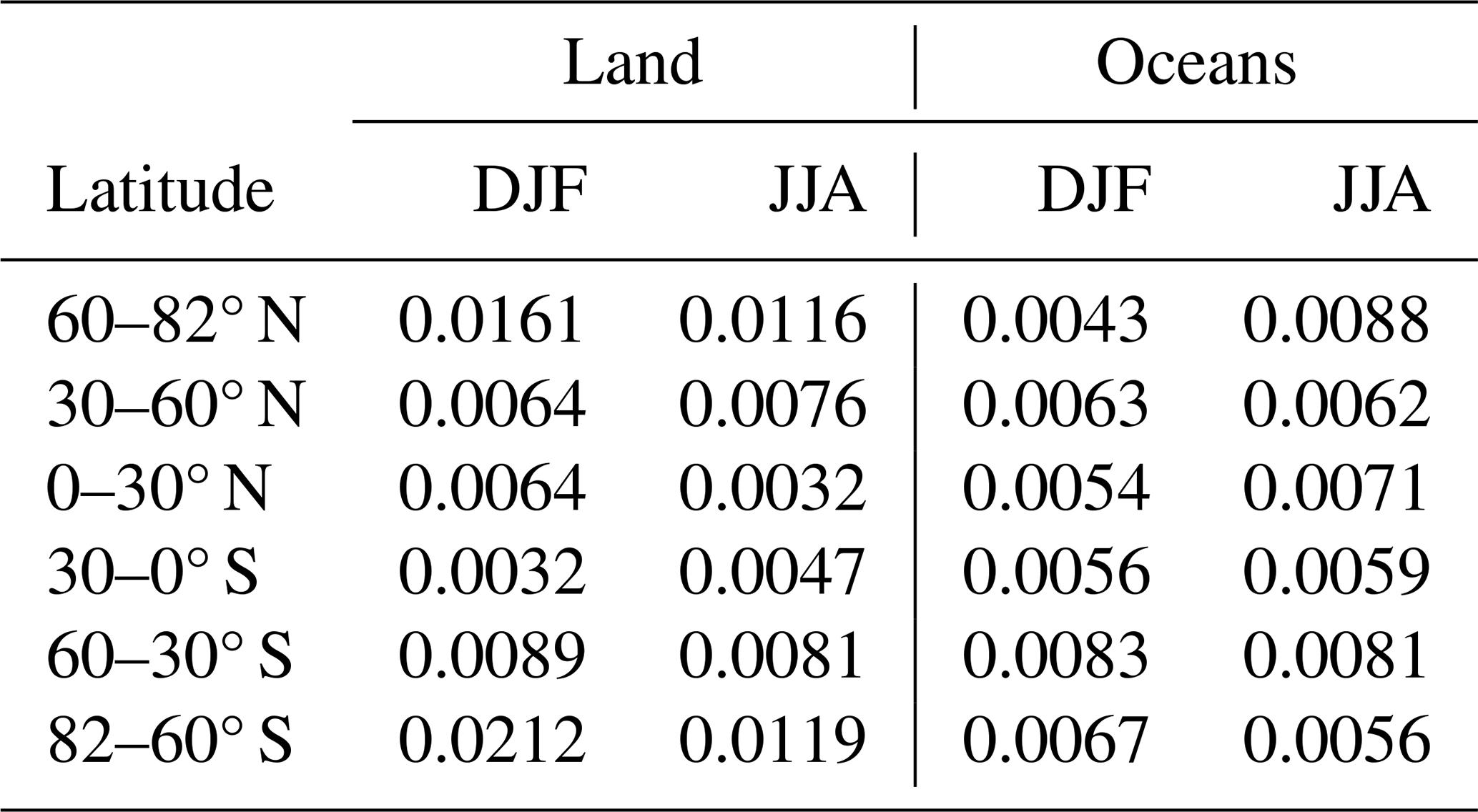
Uncertainties in ε_eff (12.05 µm) and ε_eff (10.6 µm) induce uncertainties in τ_abs (12.05 µm) and τ_abs (10.6 µm) and subsequently in β_eff. In semi-transparent clouds, the main sources of error are from the measured radiances and from the surface contribution estimates, and errors increase as effective emissivity and optical depth decrease (M2018, Garnier et al., 2021a). Errors in the surface contribution estimates are larger over land than over oceans due to the larger variability of surface emissivity and surface temperature over land. To evaluate IIR τ_abs (12.05 µm), we use CALIOP 532 nm layer integrated attenuated backscatter (IAB), which is an independent and measured quantity related to visible optical depth. Even though the relationship between CALIOP IAB and IIR τ_abs (12.05 µm) depends on Q_abs,eff (12 µm), the extinction-to-backscatter lidar ratio, and the contribution of multiple scattering to the lidar backscatter (Garnier et al., 2015), CALIOP IAB is a reliable reference to assess IIR retrieval errors as optical depth and IAB tend to zero. Furthermore, CALIOP IAB uncertainties are not sensitive to land–ocean differences. Figures 1 and 2 show median IIR τ_abs (12.05 µm) and percentiles vs. CALIOP IAB in six latitude bands over land and oceans, respectively, during December–January–February (DJF) and June–July–August (JJA) of 2008, 2010, 2012, and 2013. The statistics are built using IAB bins of $\mathrm{5}\times {\mathrm{10}}^{-\mathrm{4}}$ sr⁻¹ up to IAB = 0.02 sr⁻¹ including non-physical τ_abs (12.05 µm) negative values resulting from retrieval errors. Because most of the samples have IAB > 5 × 10⁻⁴ sr⁻¹, the lowest bin is from 5 × 10⁻⁴ to 10⁻³ sr⁻¹ where median IAB is ∼ 7.6 × 10⁻⁴ sr⁻¹. As CALIOP IAB tends to zero, median τ_abs (12.05 µm) tends to zero as expected, both over land and over oceans. To IAB = 7.6 × 10⁻⁴ sr⁻¹ corresponds a visible optical depth (τ) ∼ 0.016–0.026 assuming an extinction-to-backscatter lidar ratio between 21 and 35 sr⁻¹ (Young et al., 2018), that is median τ_abs (12.05 µm) ∼ 0.0058–0.013 assuming Q_abs,eff between 0.72 and 0.96 (see Eq. 8 and Sect. 3). The median τ_abs (12.05 µm) values in the lowest bin listed in Table 1 are ∼ 0.0091 ± 0.0054 over land and ∼ 0.0065 ± 0.0013 over oceans. This is consistent with expectations and therefore shows no evidence of bias in the retrievals. Over land, the largest discrepancy is at 82–60° S in DJF where median τ_abs (12.05 µm) might be too large by ∼ 0.01. Otherwise, the discrepancies are smaller than ± 0.003. Over oceans, the largest discrepancy is at 60–82° N in DJF where median τ_abs (12.05 µm) might be too small by ∼ 0.002. The spread of τ_abs (12.05 µm) values at a given IAB is clearly larger over land in Fig. 1 than over oceans in Fig. 2 in the smaller range of IABs and up to IAB = 0.02 sr⁻¹ in winter in the polar regions, which is due to the larger IIR uncertainties over land resulting from the variability of surface conditions. The τ_abs dispersions over land at high latitudes are approximately twice during winter relative to summer, which might be related to larger uncertainties in surface and atmospheric parameters and smaller radiative contrast between the surface and the cloud temperature.

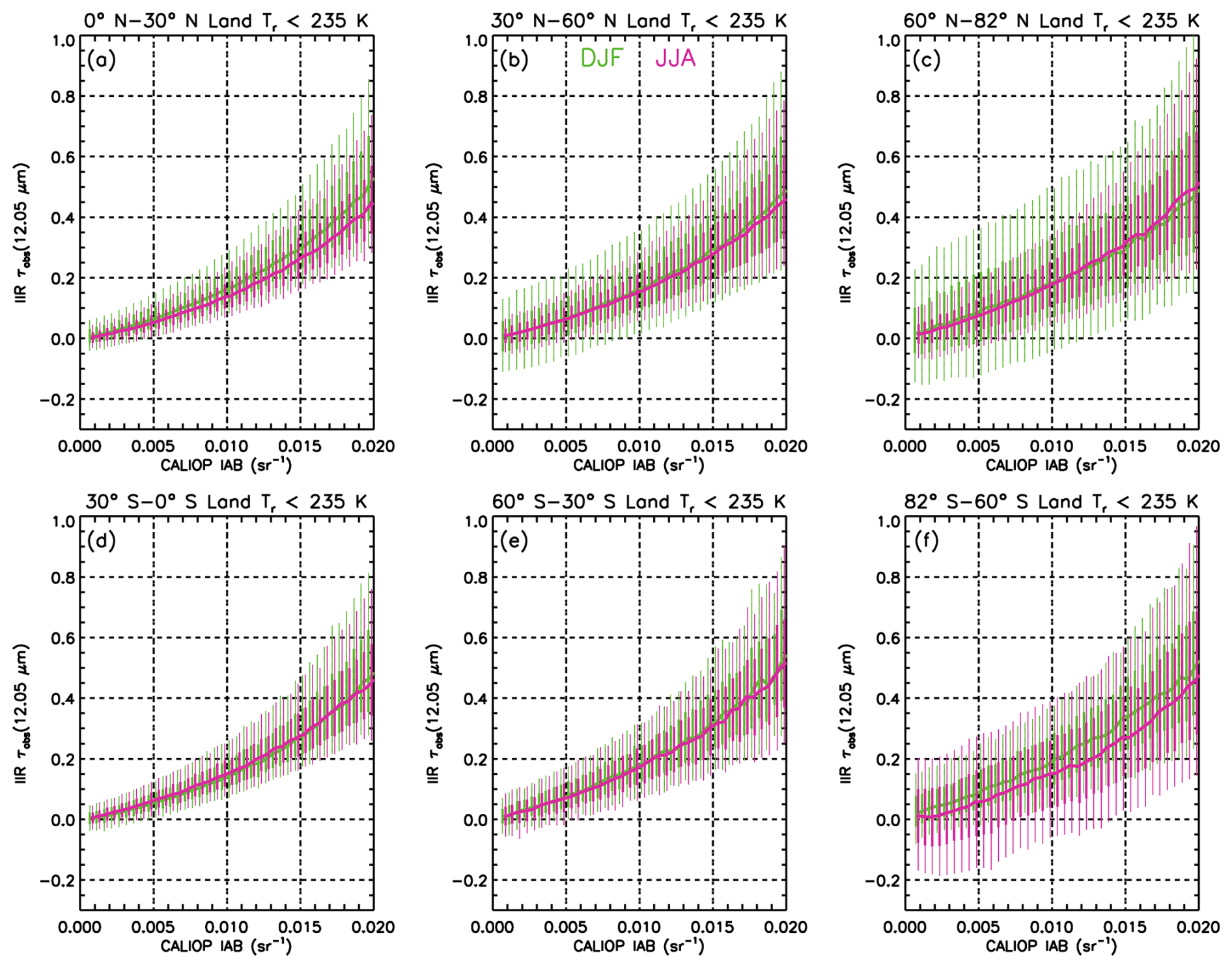
Figure 1 IIR τ_abs (12.05 µm) vs. CALIOP IAB over land in December–January–February (DJF, green) and in June–July–August (JJA, magenta). The solid curves show medians. The thin vertical lines are between the 10th and 90th percentiles and the superimposed thick lines are between the 25th and 75th percentiles. Each row features the tropics (0–30°, panels a, d), midlatitudes (30–60°, panels b, e), and high latitudes (60–82°, panels c, f) in the northern (panels a–c) and in the southern (panels d–f) hemisphere during 2008, 2010, 2012 and 2013.

Figure 2 Same as Fig. 1 but over oceans.

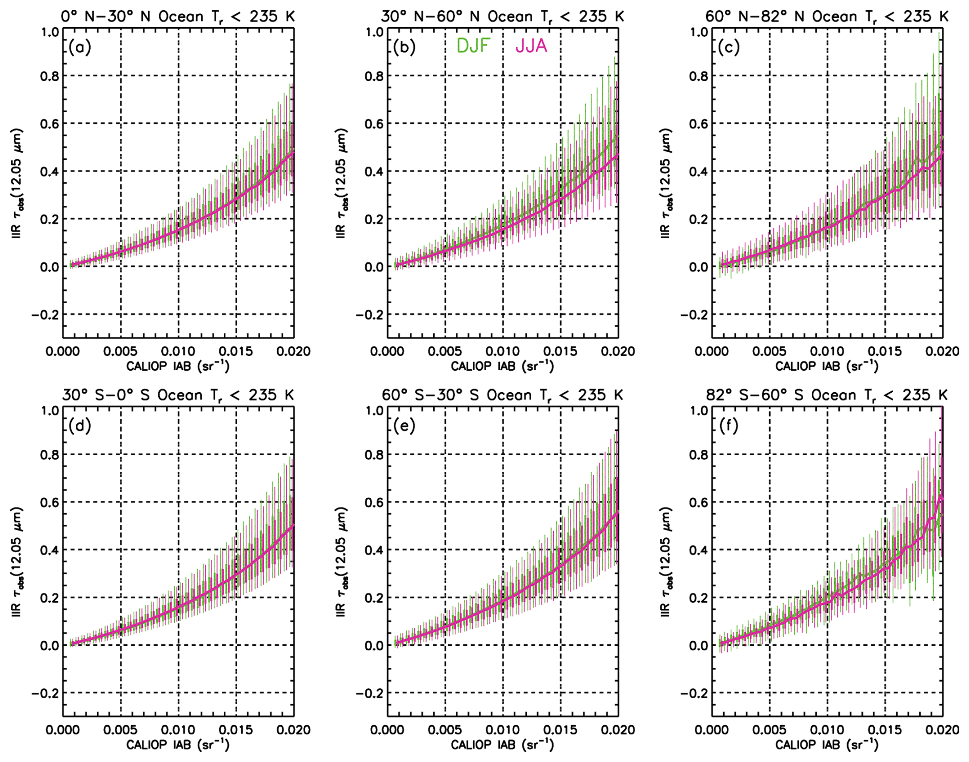
Table 1 Median IIR τ_abs (12.05 µm) in the lowest bin at CALIOP IAB ∼ 7.6 × 10⁻⁴ sr¹ using all retrievals (cf Figs. 1 and 2).

2.2.4 Impact of optical depth uncertainties in β_eff and measurement thresholds

Uncertainties in β_eff are driven by optical depth uncertainties at 12.05 and 10.6 µm. In addition to the random noise, inter-channel biases of the retrievals could yield systematic biases in β_eff, which need to be assessed. A first approach is to evaluate the median τ_abs (12.05 µm) − τ_abs (10.6 µm) differences (hereafter τ_abs12–10) when IAB tends to 0, i.e., in the lowest bin at CALIOP IAB ∼ 7.6 × 10⁻⁴ sr¹ and using all retrievals. Since the imaginary index of refraction (a measure of absorption efficiency) at 10.6 µm is lower than at 12.05 µm, we expect positive differences. The results in Appendix A show that the median differences are overall consistent with expectations, thereby showing no evidence of detectable biases.

However, β_eff can be computed only when τ_abs (12.05 µm) and τ_abs (10.6 µm) have physical positive values. Therefore, because of retrieval random errors, especially over land, the τ_abs (12.05 µm) and τ_abs (10.6 µm) distributions are truncated when computing β_eff, because the scatter around median τ_abs at low IAB values will tend to be more negative at 10.6 µm relative to 12.05 µm. To illustrate the impact of these truncations, Fig. 3 shows the median τ_abs (12.05 µm) −τ_abs (10.6 µm) differences vs. IAB over land for all retrievals (solid lines) and for samples having only positive values for both τ_abs (12.05 µm) and τ_abs (10.6 µm) (dashed line) for which β_eff can be retrieved. These β_eff values are also shown (diamonds) and are given by the right-hand axis values. Figure 4 is the same as Fig. 3 but for retrievals over oceans.

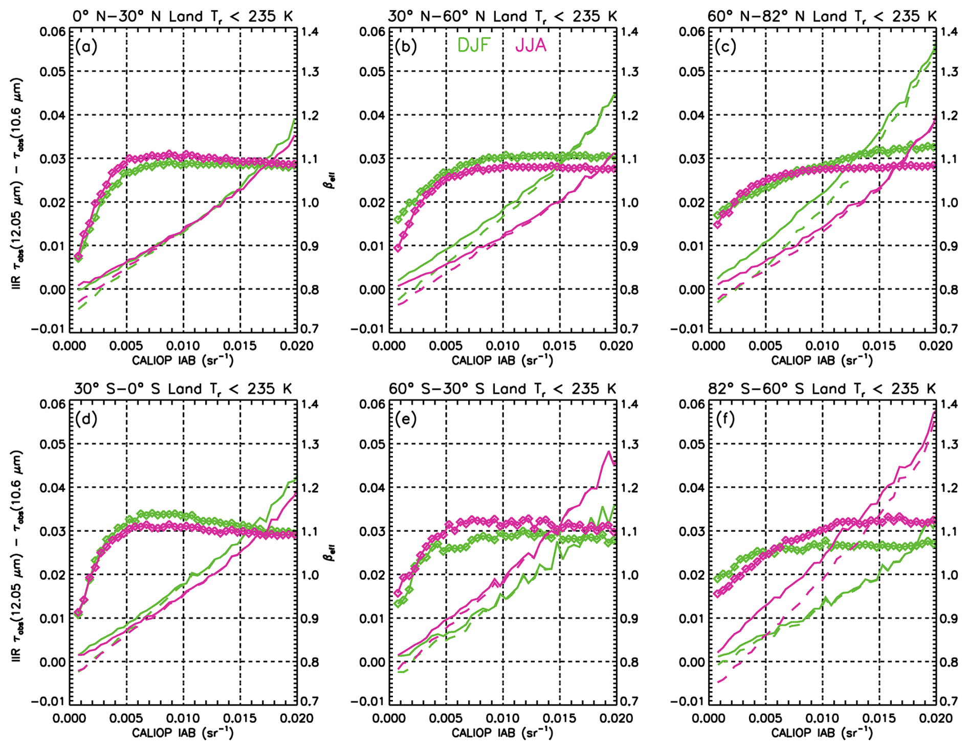
Figure 3 Median τ_abs (12.05 µm)−τ_abs (10.6 µm) difference vs. CALIOP IAB over land for all samples (solid), and for samples with positive absorption optical depths (dashed) for which β_eff (diamonds, right-hand vertical axis) can be retrieved. Each row features the tropics (0–30°, panels a, d), midlatitudes (30–60°, panels b, e), and high latitudes (60–82°, panels c, f) in the northern (panels a–c) and in the southern (panels d–f) hemisphere during December–January–February (DJF, green) and June–July–August (JJA, magenta) of 2008, 2010, 2012 and 2013.

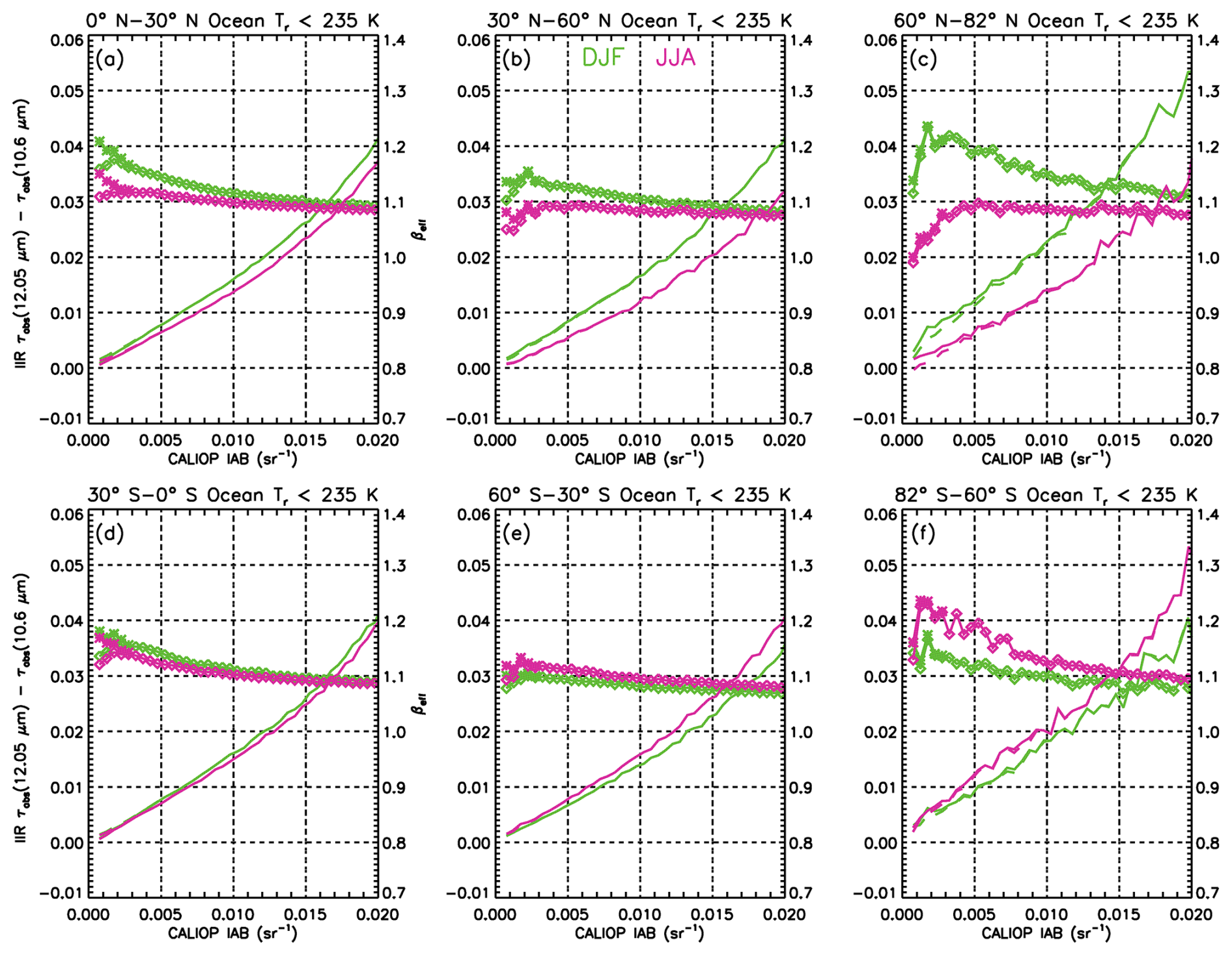
Figure 4 Same as Fig. 3 but over oceans. In addition, the differences between the asterisks and the diamonds show that requiring τ_abs (12.05 µm) ≥0.006 or visible optical depth $>\sim$ 0.01 increases median β_eff at IAB ≤0.002 sr⁻¹.

The comparison of the solid and dashed lines in Fig. 3 over land shows that discarding non-physical absorption optical depths yields underestimated optical depth differences, and therefore underestimated β_eff values. These systematic low biases result largely from the greater percentage of negative values in the dispersion around τ_abs (10.6 µm) at low IAB, so that using only the positive values yields a smaller (or negative) difference for τ_abs (12.05 µm) minus τ_abs (10.6 µm).

The greater separation between the solid and dashed curves in Fig. 3 during polar winter may relate to a lower contrast between the surface and cloud radiances and/or overall weaker radiances. But more generally, the divergence between these curves relates to the truncation bias noted above. Moreover, the decrease in β_eff with decreasing IAB for IAB < 0.01 sr⁻¹ in Fig. 3 in the polar regions, and IAB < 0.005 sr⁻¹ elsewhere, tends to roughly correspond with the divergence between the solid and dashed curves. These two trends are largely absent over oceans (cf. Fig. 4) where surface emissivity and temperature are well characterized, thus greatly reducing the amount of scatter around the median values of τ_abs (10.6 µm) and τ_abs (12.05 µm). The only exception is at high latitude in the northern hemisphere (Fig. 4c) for both seasons where β_eff at IAB smaller than 0.003 sr⁻¹ appears to be underestimated.

From this analysis, we chose a threshold IAB > 0.01 sr⁻¹ over land to ensure that the distributions are not or only slightly truncated. Nevertheless, for high latitudes in winter, median β_eff is probably underestimated for IAB up to 0.02 sr⁻¹. The chosen IAB > 0.01 sr⁻¹ threshold corresponds to median τ_abs (12.05 µm) ∼ 0.15 (Figs. 1 and 2), that is τ > ∼ 0.24–0.3 on average.

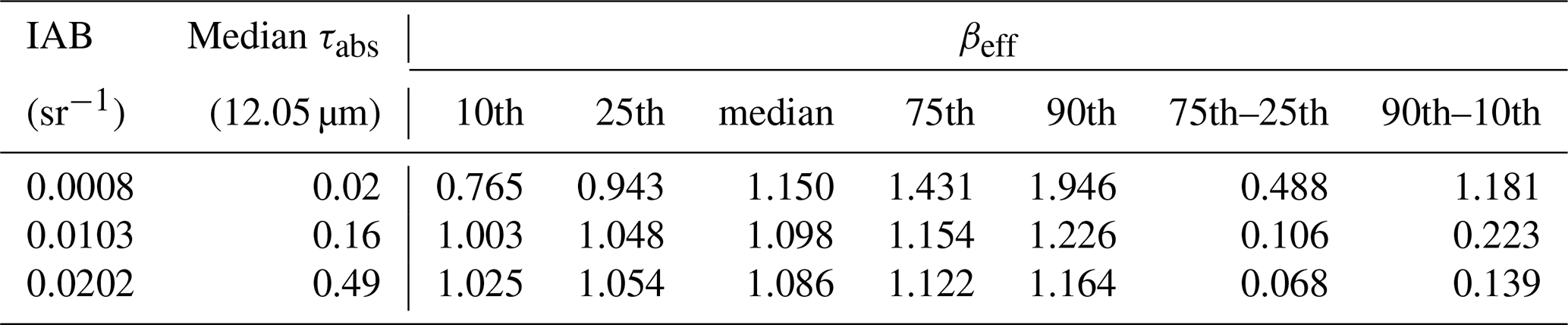
In M2018, an IAB threshold of 0.01 sr⁻¹ was applied to all retrievals, both over land and oceans. However, Fig. 4 shows that this condition can be relaxed over oceans. We refined the analysis over oceans by inspecting the fraction of negative τ_abs (10.6 µm) values as τ_abs (12.05 µm) increases from zero with increments of 0.001. We estimate that the τ_abs (10.6 µm) distribution is not significantly truncated when more than 90 % of the τ_abs (10.6 µm) values are positive, yielding a lower threshold of 0.006 for τ_abs (12.05 µm) or τ > ∼ 0.01. The asterisks in Fig. 4 show that applying this threshold slightly increases median β_eff at IAB ≤ 0.002 sr⁻¹, most notably in the tropics and at mid-latitude. Nevertheless, the width of the β_eff distributions increases rapidly as IAB and optical depth approach zero, which is due in large part to increasing random uncertainties (Garnier et al., 2021b; M2018). This is illustrated in Table 2 for JJA at 0–30° N, where the difference between the 75th and 25th β_eff percentiles is ∼ 0.49 for median τ_abs (12.05 µm) = 0.02 but only ∼ 0.07 for median τ_abs (12.05 µm) = 0.49. The difference between the 90th and 10th percentiles is approximately twice these values.

Table 2 β_eff percentiles, as well as 75th–25th and 90th–10th percentiles differences for three CALIOP IAB bins over oceans where τ_abs (12.05 µm) > 0.006 (or $\mathit{\tau }>\sim$ 0.01).

2.2.5 IIR equivalent layer thickness, Δz_eq and radiative temperature

Even though the IIR is a passive instrument that retrieves layer integrated quantities such as cloud optical depth, the cloud boundaries information provided by CALIOP allows one to retrieve vertically resolved layer properties such as the layer extinction coefficient. However, the high sensitivity of CALIOP to cloud detection and the expected variability of extinction within the layer are such that only a portion of the cloud layer detected by CALIOP is “seen” by IIR. Thus, relevant for our retrievals is the IIR equivalent layer thickness, Δz_eq, which is estimated using the IIR in-cloud weighting function derived from the in-cloud 532 nm CALIOP extinction profile of vertical resolution, δz (Garnier et al., 2021a). For this analysis, we choose to use the IIR channel centered at 12.05 µm.

The effective emissivity ε_eff of a cloud composed of n vertical bins, i, from i=1 at cloud base to i=n at cloud top can be seen as the vertically integrated in-cloud IIR effective emissivity attenuated profile ε_att (i) written as

$$\begin{array}{}\text{(12)}& {\mathit{\epsilon }}_{\mathrm{att}}\left(i\right)=\mathit{\epsilon }\left(i\right){\prod }_{j=i+\mathrm{1}}^{j=n}\left(\mathrm{1}-\mathit{\epsilon }\left(j\right)\right).\end{array}$$

In Eq. (12), ε(i) is the emissivity of bin i, and the second term represents the transmittance through the overlying cloudy bins. The ε(i) term is derived from the CALIOP cloud extinction coefficient of bin i, α_part(i), as

$$\begin{array}{}\text{(13)}& \mathit{\epsilon }\left(i\right)=\mathrm{1}-\exp \left(-{\mathit{\alpha }}_{\mathrm{part}}\left(i\right)\mathit{\delta }z/r\right),\end{array}$$

where r is the scaling ratio between the CALIOP layer optical depth, τ_CAL, and the cloud effective absorption depth τ_abs. The IIR weighting function, WF_IIR(i), is obtained from Eq. (12) after normalization by ε_eff as

$$\begin{array}{}\text{(14)}& {\mathrm{WF}}_{\mathrm{IIR}}\left(i\right)={\displaystyle \frac{{\mathit{\epsilon }}_{\mathrm{att}}\left(i\right)}{{\mathit{\epsilon }}_{\mathrm{eff}}}},\end{array}$$

so that

$$\begin{array}{}\text{(15)}& {\sum }_i{\mathrm{WF}}_{\mathrm{IIR}}\left(i\right)=\mathrm{1}.\end{array}$$

Then, we compute the IIR-weighted layer extinction coefficient, α_CAL-IIR, as

$$\begin{array}{}\text{(16)}& {\mathit{\alpha }}_{\text{CAL-IIR}}={\sum }_{i=\mathrm{1}}^{i=n}{\mathit{\alpha }}_{\mathrm{part}}\left(i\right){\mathrm{WF}}_{\mathrm{IIR}}\left(i\right).\end{array}$$

This IIR-weighted layer extinction coefficient is larger than or equal to the mean layer extinction, noted mean (α_CAL). Finally, the IIR equivalent layer thickness, Δz_eq, is related to the geometric thickness Δz as

$$\begin{array}{}\text{(17)}& \mathrm{\Delta }{z}_{\mathrm{eq}}=\mathrm{\Delta }z{\displaystyle \frac{\mathrm{mean}\left({\mathit{\alpha }}_{\mathrm{CAL}}\right)}{{\mathit{\alpha }}_{\text{CAL-IIR}}}}.\end{array}$$

The ratio r in Eq. (13) is estimated using CALIOP visible optical depth, and might thus differ from $\mathrm{2}/Q_{\mathrm{abs},\mathrm{eff}}$ (12 µm) used in this study to derive visible optical depth, τ (Eq. 8). Importantly, Δz_eq does not depend on this ratio. Had we used τ instead of τ_CAL, both α_part and r in Eq. (13) would have been multiplied by $\mathit{\tau }/{\mathit{\tau }}_{\mathrm{CAL}}$ and ε(i) and the subsequent WF_IIR(i) would have been unchanged. Similarly, both mean(α_CAL) and α_CAL-IIR in Eq. (17) would have been multiplied by $\mathit{\tau }/{\mathit{\tau }}_{\mathrm{CAL}}$, leaving Δz_eq unchanged. We note, however, that without vertically resolved information, $\mathrm{2}/Q_{\mathrm{abs},\mathrm{eff}}$ (12 µm) (or r) is supposed constant within the layer.

Two cirrus examples are shown in Fig. 5 where the CALIOP extinction coefficient (α_part) profile is in black and the IIR weighting function (WF_IIR) profile is in red. The vertical resolution is δz= 0.06 km. The first example in panel (a) is a TTL cirrus between 15.13 and 16.5 km observed in June 2010. Retrieved ε_eff is equal to 0.06 and the black and red curves have an almost identical shape because the attenuation term in Eq. (12) is close to 1. We find Δz_eq= 0.52 km, which corresponds roughly to the main marked peak and to the secondary maximum. In panel (b), the cirrus is between 6.74 and 10.74 km in the Southern Ocean in August 2008. Here, retrieved ε_eff is equal to 0.44 and relative to the black curve, the lower part of the cloud contributes less to the cloud emissivity than the upper part. The equivalent thickness Δz_eq= 2.98 km can be seen as the portion of the cloud above 7.8 km where WF_IIR exceeds approximately 0.008. In these examples, $\mathrm{\Delta }{z}_{\mathrm{eq}}/\mathrm{\Delta }z$ is equal to 0.38 (a) and 0.74 (b). Figure 6 shows Δz_eq vs. Δz for all the sampled cirrus over oceans, showing that $\mathrm{\Delta }{z}_{\mathrm{eq}}/\mathrm{\Delta }z$ is globally mostly between 0.5 and 0.9.

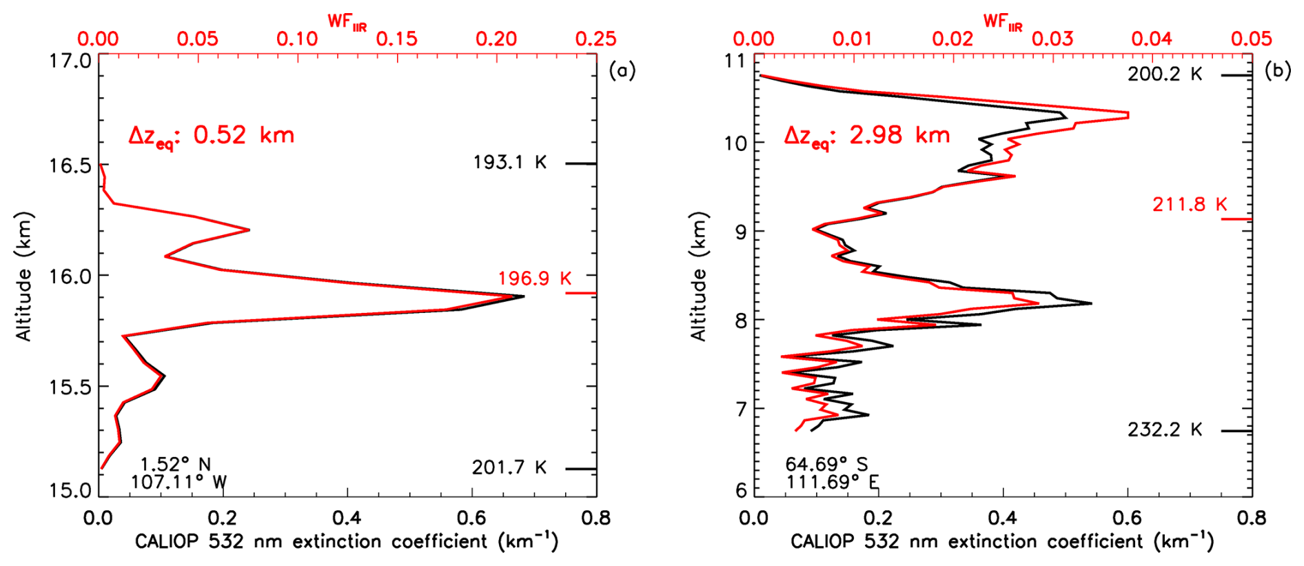
Figure 5 Two cirrus cloud examples showing the CALIOP extinction coefficient (α_part) profile in black and the IIR weighting function (WF_IIR) profile in red, with Δz_eq indicated in red. The temperatures in black on the right-hand side of each panel are at cloud top and base, and in red is the radiative temperature (T_r) at the corresponding altitude. These examples are extracted from CALIPSO granules (a) 2010-06-04T08-39-58ZN and (b) 2008-08-12T07-26-54ZD, with latitude and longitude given in the lower left-hand corner of the respective panels.

The examples shown in Fig. 5 illustrate that the IIR weighting function is in first approximation the CALIOP extinction profile normalized to the optical depth if the attenuation term in Eq. (12) is supposed to be close to 1 and ε(i) is approximated to the corresponding τ_abs in Eq. (13). This IIR weighting function is also used to determine the cloud centroid radiance and the corresponding radiative temperature, T_r (Garnier et al., 2021a), which is given in red in each panel. The temperatures in black are T_top and T_base at the layer top and base altitudes, respectively. Because computing a centroid temperature would yield a temperature differing by less than a few tenths of a degree Kelvin (M2018), T_r can be seen as the temperature dividing the cloud optical depth τ into equal parts. In panel (a) where WF_IIR exhibits one main peak, the altitude corresponding to T_r is 15.9 km, near the WF_IIR maximum. The T_r–T_top difference is 45 % of the thermal thickness. In panel (b), the altitude corresponding to T_r is 9.1 km located between the two peaks of comparable amplitude, slightly closer to the upper one. T_r is slightly closer to the top with a T_r–T_top difference of 36 % of the thermal thickness. As discussed in M2018 and illustrated in Fig. 7 showing T_r–T_top against T_base–T_top for all the sampled cirrus over oceans, T_r–T_top represents typically 30 % to 70 % of T_base–T_top. Using temperature difference as a proxy for altitude difference, it appears that T_r is on average at mid-cloud.

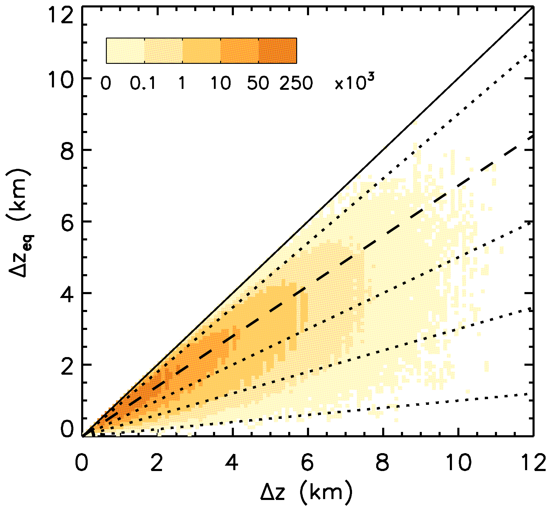
Figure 6 Δz_eq vs. Δz for all sampled cirrus over oceans during 2008, 2010, 2012, and 2013. The colors represent the IIR pixels density. The dashed and dotted lines, from bottom to top, represent $\mathrm{\Delta }{z}_{\mathrm{eq}}/\mathrm{\Delta }z$ of 0.1, 0.3, 0.5, 0.7, and 0.9.

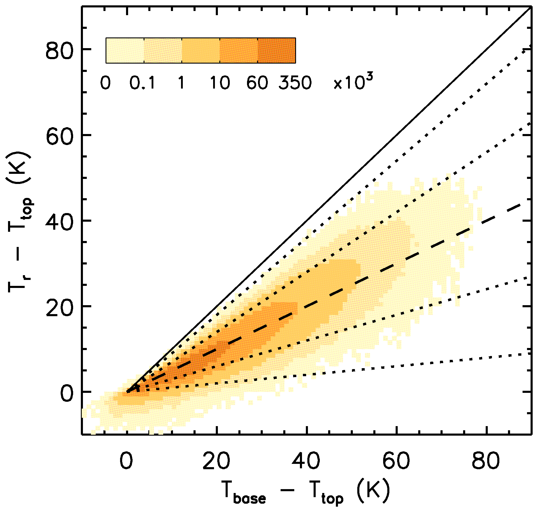
Figure 7 T_r–T_top vs. T_base–T_top for all sampled cirrus over oceans during 2008, 2010, 2012, and 2013. The colors represent the IIR pixels density. The dashed and dotted lines, from bottom to top, represent (T_r–T_top) $/$ (T_base–T_top) of 0.1, 0.3, 0.5, 0.7, and 0.9. Using temperature difference as proxy for altitude difference, it appears that T_r is on average at mid-cloud.

2.3 Inclusion of additional tropical cirrus field campaigns

The M2018 CALIPSO retrieval was based on X–β_eff relationships (where X refers to $N_{\mathrm{i}}/$ IWC, D_e, or $\mathrm{2}/Q_{\mathrm{abs},\mathrm{eff}}$ (12 µm)) developed from the SPARTICUS (Jensen et al., 2013a) and TC4 (Toon et al., 2010) cirrus cloud field campaigns. In this new retrieval, the ATTREX and POSIDON cirrus cloud field campaigns (Jensen et al., 2017; Schoeberl et al., 2019) conducted in the tropical western Pacific were also used for this purpose, along with the SPARTICUS and TC4 field campaigns. Cirrus clouds were sampled in POSIDON by the NASA WB-57 aircraft, which flew the SPEC Inc. Fast Cloud Droplet Probe (FCDP; Glienke and Mei, 2020; Lawson et al., 2017), two-dimensional stereo (2D-S) probe (Lawson et al., 2006) and Cloud Particle Imager (CPI; Lawson et al., 2001). During ATTREX, they were sampled by the Global Hawk uncrewed aircraft system, which flew the SPEC Inc. Hawkeye instrument to measure ice PSDs between −50 and −85 °C but mostly in the TTL between −65 and −85 °C (Woods et al., 2018). The Hawkeye houses three instruments that measure the complete cloud PSD and the corresponding size-resolved cloud particle shapes; these are versions of the FCDP, the 2D-S probe and the CPI. The FCDP and 2D-S probe tips are designed to minimize ice particle shattering, and particle interarrival times are used to identify and remove clusters of particles resulting from shattering (Baker et al., 2009). The FCDP sampled particles between 1 and 50 µm while the 2D-S sampled ice particle maximum dimension D from 10 to 1280 µm (Woods et al., 2018), although D>1280 µm can be estimated up to 4 mm (Jensen et al., 2017). However, the first (5–15 µm) size bin of the 2D-S probe and the last size bin (45–50 µm) of the FCDP were not used for producing composite mean PSDs. Figure 8 shows representative mean PSD examples from POSIDON (on left) and ATTREX (on right) along with information on corresponding effective radius (R_eff), N_i, and IWC. The agreement between the FCDP and 2DS probes where they overlap (from 15 to 45 µm, indicated by the red and blue histograms) was good (as shown here) for most of the PSD measurements. The number of PSDs during POSIDON having notably poorer agreement than those in Fig. 8 was 3 out of 66 PSDs in total, or 4.5 %, with similar findings for ATTREX. Moreover, Jensen et al. (2013a) found good agreement for N_i between the 2D-S and another N_i probe (the Video Ice Particle Sampler or VIPS) when the first size bin of the 2D-S probe was not considered.

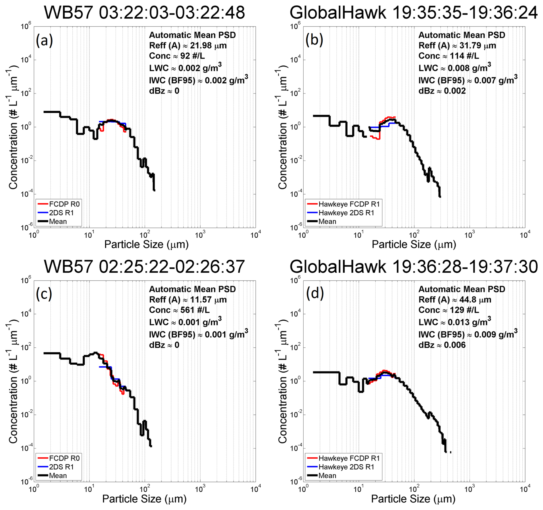
Figure 8 Representative mean composite PSD from the ATTREX (b, d) and POSIDON (a, c) field campaigns, sampled by the FCDP (1.5–45 µm) and 2D-S (15–1280 µm) probes. The two probes in their overlap region (red and blue histograms) yield relatively consistent values, providing confidence in these measurements.

For the SPARTICUS and TC4 campaigns, PSDs were measured only by the 2D-S probe. To determine whether ice particle concentrations in the first size bin (i.e., N(D)₁) of the 2D-S probe should be used for calculating the $N_{\mathrm{i}}/$ IWC–β_eff, $N_{\mathrm{i}}/A_{\mathrm{PSD}}$–β_eff and $\mathrm{1}/Q_{\mathrm{abs},\mathrm{eff}}$ (12 µm)–β_eff relationships from these campaigns (that were used in this retrieval as described in Sect. 3), PSDs from the POSIDON campaign were qualitatively evaluated from PSD plots provided by SPEC, Inc. The good agreement noted above between the FCDP and 2D-S probes from 15 to 45 µm suggests that the FCDP measurements from 1 to 15 µm may also be realistic. Jensen et al. (2013a) states that “In nearly all of the 2D-S size distributions, the concentration in the first size bin (5–15 µm) is considerably larger than the concentrations in the next few larger bins, and the first bin often contributes significantly to the overall ice concentration.” We found this to be true of the ATTREX-POSIDON 2D-S measurements as well. For the POSIDON PSDs, N(D)₁ of the 2D-S was within a factor of ∼ 2.5 of the combined corresponding FCDP bins for 23 % of the PSDs but exhibited much higher factors ranging from 3 to 32 for the other PSDs. On average, the 2D-S N(D)₁ was a factor of 10.4 ± 8.1 greater than the ice particle concentration in the corresponding FCDP bins. Therefore, regarding the SPARTICUS and TC4 PSDs, we modified the measured PSDs by dividing the 2D-S N(D)₁ by 10.4 to approximately correct for this behavior. While this correction would not always be valid for a single PSD measurement, it may be realistic for a large ensemble of PSDs. Relevant information for the SPARTICUS and TC4 field campaigns can be found in M2018. In M2018, different assumptions regarding N(D)₁ resulted in different retrieval formulations, but in the current approach, only one retrieval formulation is needed and presented.

2.4 Treatment of ice water content

As shown in Fig. 8, ATTREX and POSIDON PSDs were generally narrow, with maximum ice particle sizes generally less than 400 µm and often less than 150 µm. The Baker and Lawson (2006) ice particle area-mass expression that has normally been used to calculate the IWC for SPEC, Inc. PSD data predicts a spherical ice particle mass greater than predicted for spherical ice particles at bulk ice density (0.917 g cm⁻³) when ice particle maximum dimension D<47 µm (which is non-physical). Since much of the PSD mass during the ATTREX and POSIDON campaigns is often associated with D<47 µm, the ice particle mass-dimension expressions described in Erfani and Mitchell (2016; henceforth EM2016) were used for developing relationships in this retrieval scheme since the EM2016 mass-dimension relationships were designed to calculate the mass of small particle sizes <100 µm more realistically. These EM2016 relationships are shown in Fig. 9, along with relationships from Lawson et al. (2019) for marine anvils cirrus, from Mitchell et al. (2010), and from Weitzel et al. (2020). It is seen that these relationships are relatively consistent, especially for D<100 µm where uncertainties are greatest.

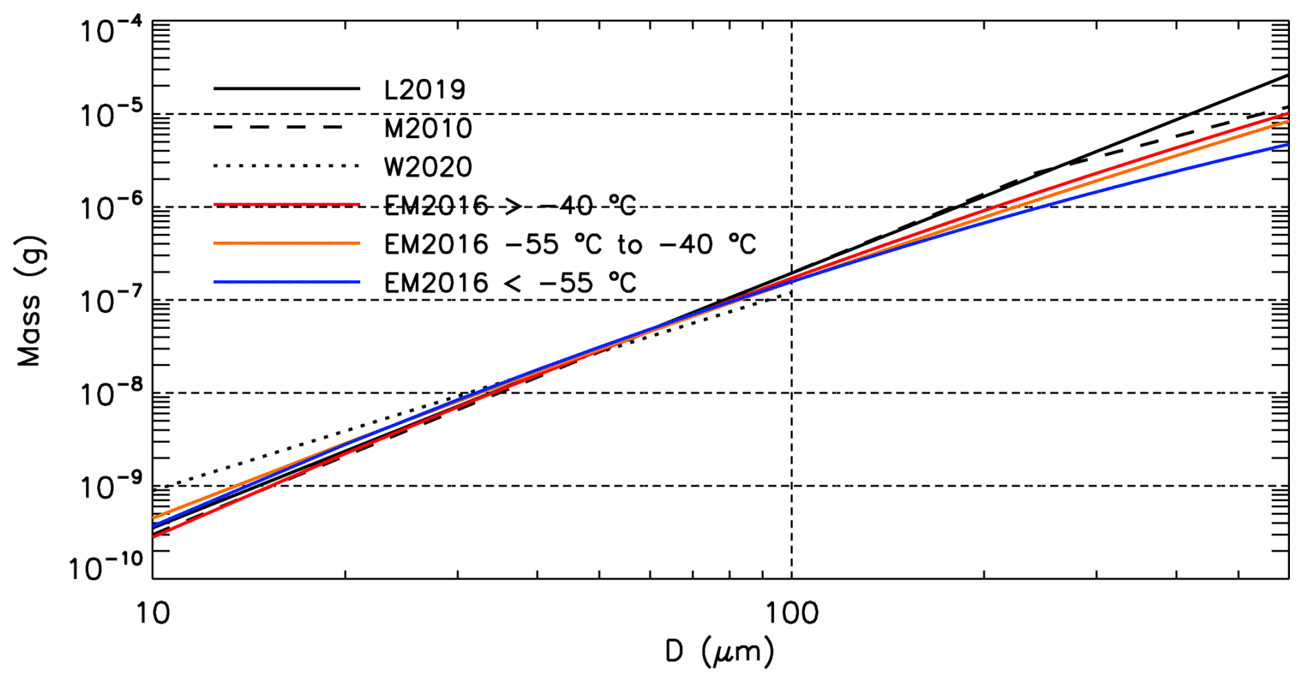
Figure 9 Relationships between mass m (g) and particle dimension D (µm) from Lawson et al. (2019) (L2019, solid black line), Mitchell et al. (2010) (M2010, dashed black line), Weitzel et al. (W2020, dotted black line), and from EM2016 for temperatures colder than 55 °C (blue), between −55 and −40 °C (orange) and warmer than −40 °C (red).

2.4.1 Mass-dimension relationship and β_eff

We recall that β_eff of the PSD is the ratio of effective absorption efficiencies at 12.05 and 10.6 µm, where “effective” refers to the scattering contribution (see Eqs. 4 and 5 of M2018). For this discussion, we can assume that β_eff ∼ β, i.e., the ratio of absorption efficiencies at 12.05 and 10.6 µm. As discussed in Mitchell (2002), the relevant dimension to characterize the absorption efficiency of the single particle at a given wavelength, λ, is the effective distance d_e defined as

$$\begin{array}{}\text{(18)}& d_{\mathrm{e}}={\displaystyle \frac{m}{{\mathit{\rho }}_{\mathrm{i}}\cdot A_{\mathrm{p}}}}.\end{array}$$

Similarly, absorption efficiencies, q_abs (λ), derived from MADA are uniquely related to d_e, as shown in Fig. 10a for the IIR channels using several ATTREX and POSIDON PSDs. The x-axis is ($\mathrm{3}/\mathrm{2}$) × d_e, noting that this quantity is the effective diameter of the single particle. While A_p is directly measured, m is derived from mass-dimension or mass-area relationships, so that d_e depends on these relationships. The discontinuities in q_abs (λ) result from changes in the MADA tunneling (i.e., resonance) efficiencies that depend on ice particle shape and size (M2018; Sect. 2.3). The PSD absorption efficiency Q_abs (λ) is obtained after integration of q_abs (λ) over the area distribution, A(D), where D is particle dimension. Because q_abs (λ) is uniquely related to d_e, Q_abs (λ) can be written

$$\begin{array}{}\text{(19)}& Q_{\mathrm{abs}}\left(\mathit{\lambda }\right)={\int }_{\mathrm{PSD}}{q}_{\mathrm{abs}}(\mathit{\lambda },d_{\mathrm{e}}(D\left)\right)A\left(D\right)\mathrm{d}D\end{array}$$

and

$$\begin{array}{}\text{(20)}& \mathit{\beta }={\displaystyle \frac{Q_{\mathrm{abs}}\left(\mathrm{12}\mathrm{\mu }\mathrm{m}\right)}{Q_{\mathrm{abs}}\left(\mathrm{10.6}\mathrm{\mu }\mathrm{m}\right)}}.\end{array}$$

It appears that Q_abs (λ) and β of a PSD depend on the variation of A(D) with d_e, which again depends on the estimated mass of the single particle. This is illustrated in Fig. 10b–d with three examples from the ATTREX and POSIDON campaigns, where the same A(D) is shown vs. ($\mathrm{3}/\mathrm{2}$) × d_e using the mass from EM2016 (shown black) and from SPEC (shown red). The black distributions are shifted towards smaller d_e values compared to the red ones, yielding a larger β (and ultimately β_eff) value using the EM2016 relationships. In these examples, the β_eff values are increased from 1.059 to 1.091 in panel (a), from 1.088 to 1.192 in panel (b) and from 1.191 to 1.316 in panel (c).

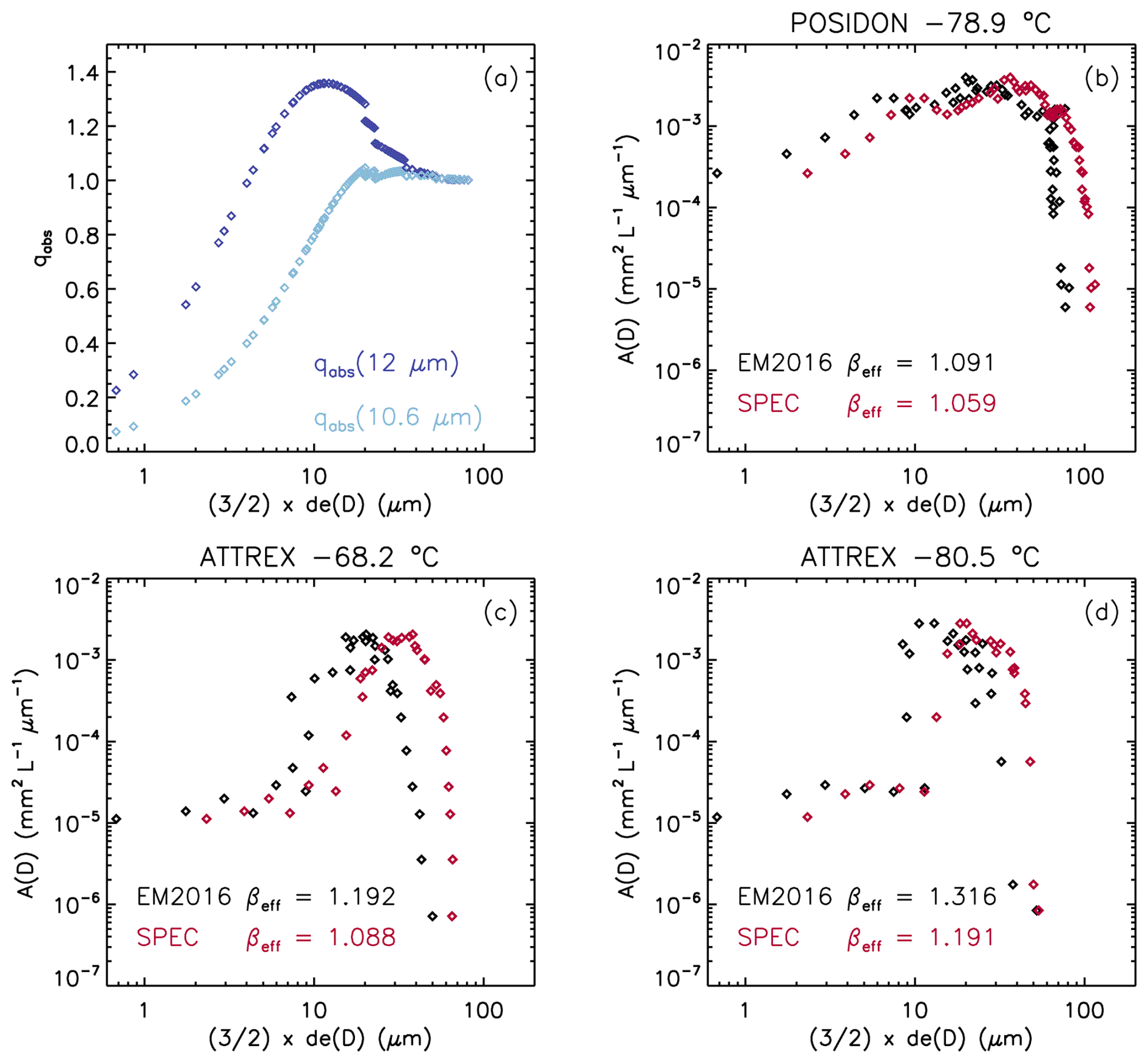
Figure 10 Panel (a) shows the unique relationship between absorption efficiency at 12 µm (dark blue) and 10.6 µm (light blue) and effective distance d_e (D). Panels (b)–(d) show three examples of A(D) vs. ($\mathrm{3}/\mathrm{2}$) × d_e(D) from the POSIDON (b) and the ATTREX (c)–(d) campaigns with d_e(D) computed using particle mass from EM2016 (black) and SPEC (red). The smaller mass using EM2016 yields smaller d_e(D) and larger β_eff values.

2.4.2 IIR β_eff – temperature comparisons with SPEC and EM2016

To assess the impact of the m–D relationships on in situ β_eff, we compared β_eff of PSDs measured during the ATTREX (2014) and POSIDON campaigns with independent IIR β_eff retrievals (Fig. 11). Because one-to-one comparisons are not possible, we compared β_eff vs. temperature, which is layer radiative temperature for IIR. To match the field campaigns, IIR samples are in 0–20° N and 130–160° E during February and March 2014 for ATTREX and October 2016 for POSIDON (Schoeberl et al., 2019). Comparisons in Fig. 11 are for IIR single-layer semi-transparent cirrus clouds having IAB > 0.01 sr⁻¹ or τ > ∼ 0.3. Most of the PSD β_eff derived using the SPEC relationships are smaller than median IIR β_eff, whereas using the EM2016 relationships brings PSD and IIR β_eff values in a good agreement. However, because the field campaigns targeted TTL cirrus clouds, most of the PSD temperatures are colder than 208 K whereas IIR sampling is sparse below 200 K. As the sampled region is over oceans, we repeated the experiment in Fig. 12 but this time by including cloud having τ∼ 0.01. IIR sampling of TTL clouds is improved in Fig. 12, so that the comparisons are more informative. Despite the increased random noise, which explains the larger occurrence of extreme IIR β_eff values in Fig. 12 than in Fig. 11, IIR and PSD β_eff are again in better agreement for the EM2016 relationships. The horizontal dashed light blue lines in the left-hand panels of Figs. 11 and 12 indicate β_eff at the sensitivity limit (see Sect. 3).

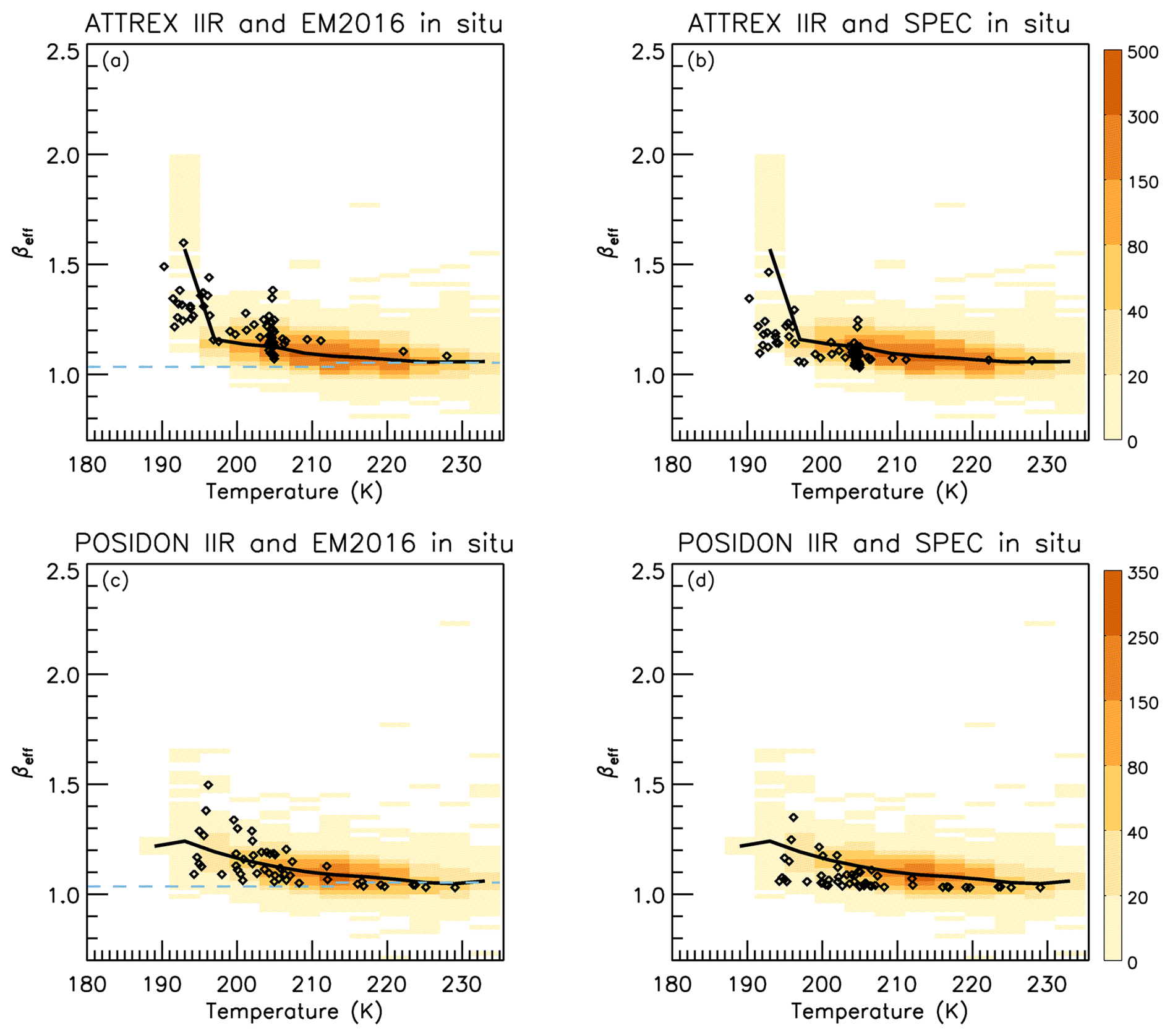
Figure 11 IIR β_eff vs. temperature in 0–20° N and 130–160° E during February and March 2014 (ATTREX, panels a, b) and October 2016 (POSIDON, panels c, d) compared with β_eff of PSDs (diamonds) measured during the denoted campaigns using the EM2016 (panels a, c) and the SPEC (panels b, d) mass-dimension relationships. The colors indicate IIR samples density and black curves represent median IIR β_eff. The horizontal dashed light blue lines in panels (a) and (c) indicate β_eff at the sensitivity limit (see Sect. 3). IIR optical depth > ∼ 0.3.

3 Relationships used in the retrieval

3.1 Correction of the smallest bin of the 2D-S probes and mass-dimension relationship

As discussed in Sect. 2.3, a modification of the smallest bin of the PSDs is needed for the SPARTICUS and TC4 campaigns where only the 2D-S probe was used. The correction was determined from the analysis of PSDs measured during the ATTREX and POSIDON campaigns since the FCDP was used over the ice particle size-range corresponding to the smallest 2D-S bin. In addition, based on the findings presented in Sect. 2.4, we now use the EM2016 mass-dimension relationships.

It is instructive to examine the impact of these changes in terms of the N_i retrieval as described in Eq. (2). The field campaign dependence (and thus the 2D-S probe dependence) of N_i enters through the β_eff dependent terms in Eq. (2), that is, through the $N_{\mathrm{i}}/A_{\mathrm{PSD}}$–β_eff and the [$\mathrm{1}/Q_{\mathrm{abs},\mathrm{eff}}$ (12 µm)]–β_eff relationships. From Eq. (2), the product of these two ratios is $N_{\mathrm{i}}/{\mathit{\alpha }}_{\mathrm{abs}}$ which is plotted in Fig. 13, showing the impact of the mass-dimension relationships and of the N(D)₁ assumption on the N_i retrieval. There are three assumptions: (1) N(D)₁ is unmodified, meaning the N(D)₁ measurement is correct, (2) N(D)₁ is modified, divided by 10.4 as discussed in Sect. 2.3, and (3) N(D)₁= 0. These three assumptions were evaluated in Fig. 13 using 2D-S PSD data from the SPARTICUS field campaign measured at temperatures less than −38 °C using the EM2016 relationships. Assumption (1) as derived in M2018 is also shown in black, showing that using the EM2016 relationships (in purple) reduces retrieved N_i. Taking the modified assumption (in navy blue) to be most realistic, it is seen that either assumption (1) or (3) can produce significant errors. Moreover, this reveals the N_i retrieval sensitivity to the size bin for the smallest ice particles. It was fortuitous that both the FCDP and 2D-S probes were flown during the ATTREX and POSIDON field campaigns, which enabled the estimation of a correction factor. Hence forward, only the modified assumption is used for N(D)₁ for both SPARTICUS and TC4.

Figure 12 Same as Fig. 11 but using IIR optical depth > ∼ 0.01.

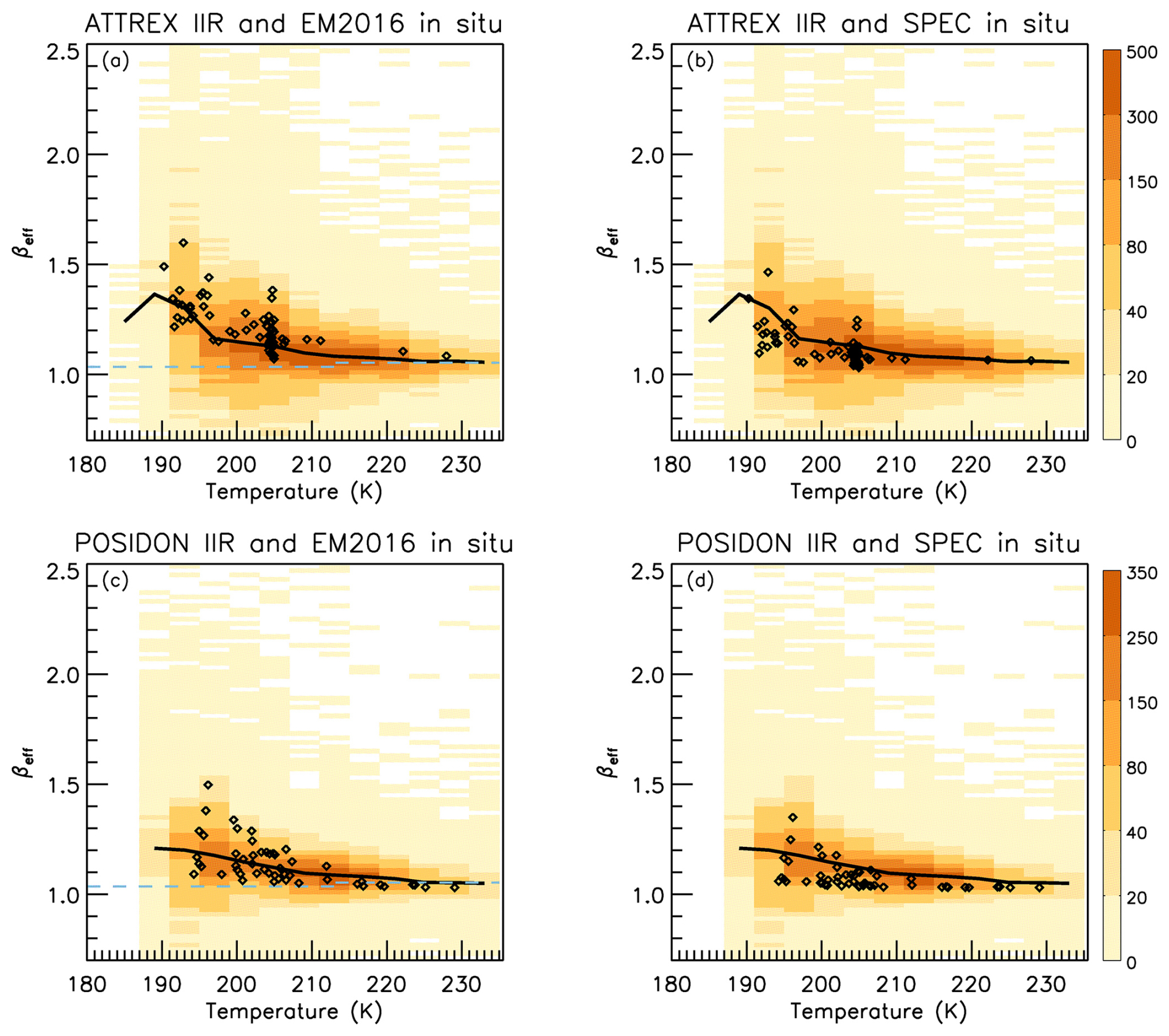
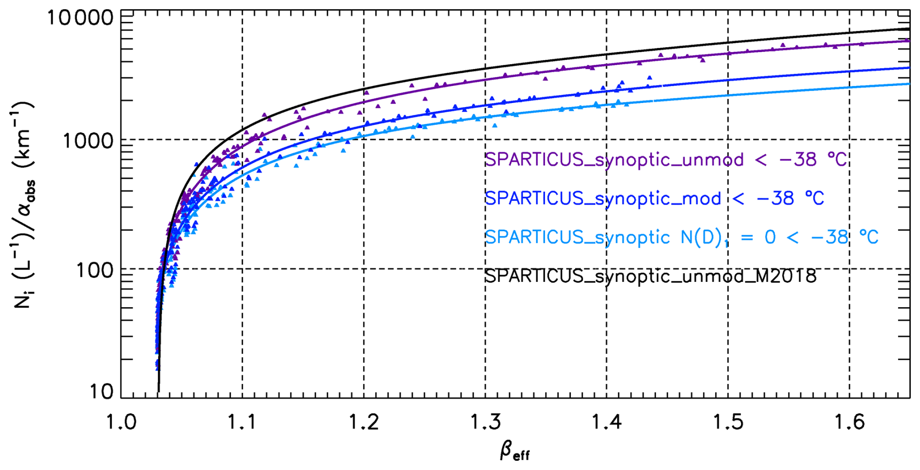
Figure 13 Sensitivity of the SPARTICUS N_i retrieval using the EM2016 mass-dimension expressions to assumptions concerning the first size bin of the 2D-S probe, N(D)₁, which can either be unmodified (purple), modified (by dividing N(D)₁ by 10.4, navy blue), or set equal to zero (light blue). The black curve is the relationships for N(D)₁ unmodified from M2018. See text for details.

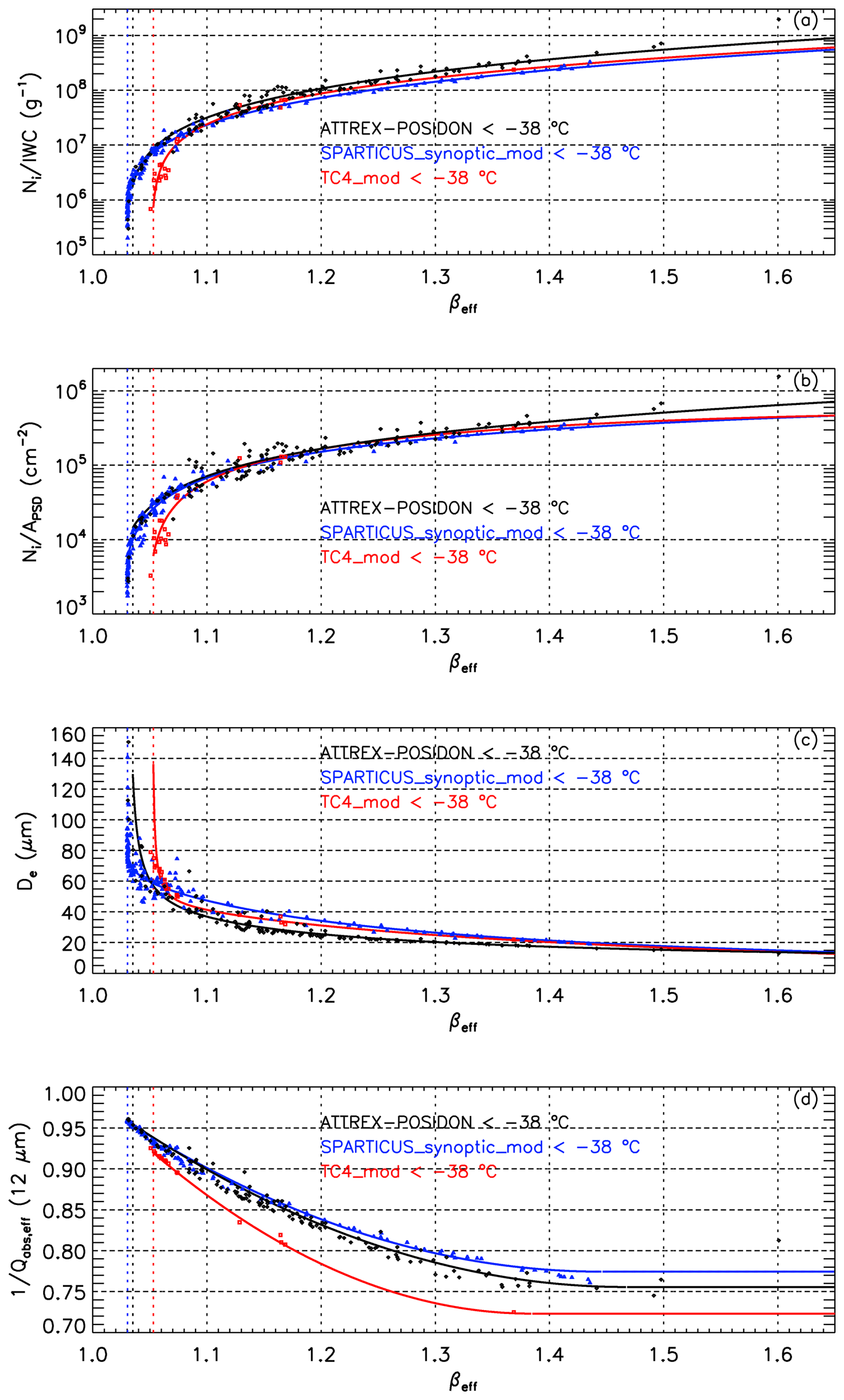
Figure 14 The dependence of this retrieval on β_eff is comprised of the above four types of relationships. The curve fits shown correspond to the ATTREX-POSIDON (black), SPARTICUS (navy blue) and TC4 (red) field campaigns where SPARTICUS is based on synoptic cirrus clouds and N(D)₁ was modified for SPARTICUS and TC4. Data points were calculated from the PSD samples having temperature less than −38 °C with colors indicating the respective field campaign.

3.2 Relating β_eff to $N_{\mathrm{i}}/$ IWC, $N_{\mathrm{i}}/A_{\mathrm{PSD}}$, D_e, and $\mathrm{1}/Q_{\mathrm{abs}}$ (12 µm)

The X–β_eff relationships used in the retrieval Eqs. (2), (4) and (7) where X is $N_{\mathrm{i}}/A_{\mathrm{PSD}}$, $N_{\mathrm{i}}/$ IWC and $\mathrm{1}/Q_{\mathrm{abs}}$ (12 µm), respectively, are shown in Fig. 14 along with the β_eff dependence of D_e which is based on Eq. (4). The solid lines in panels (a), (b) and (d) are second-order polynomial curve fits based on the indicated field campaigns where both X and β_eff are calculated from PSD measurements and MADA (in the case of $\mathrm{1}/Q_{\mathrm{abs}}$ and β_eff). The solid lines in panel (c) are based on Eq. (4). PSDs from the ATTREX and POSIDON field campaigns are mostly from TTL cirrus and were sampled using the same instruments in the tropical western Pacific; therefore, they were combined as a single dataset. While the SPARTICUS data were subdivided into anvil cirrus and synoptic cirrus (i.e., any cirrus not associated with convection), only the curve fits for synoptic cirrus were used since they represented both cirrus types well. All the PSDs used to produce Fig. 14 were measured at temperatures less than −38 °C. The IWCs and β_eff values were calculated using the m-D expressions in EM2016.

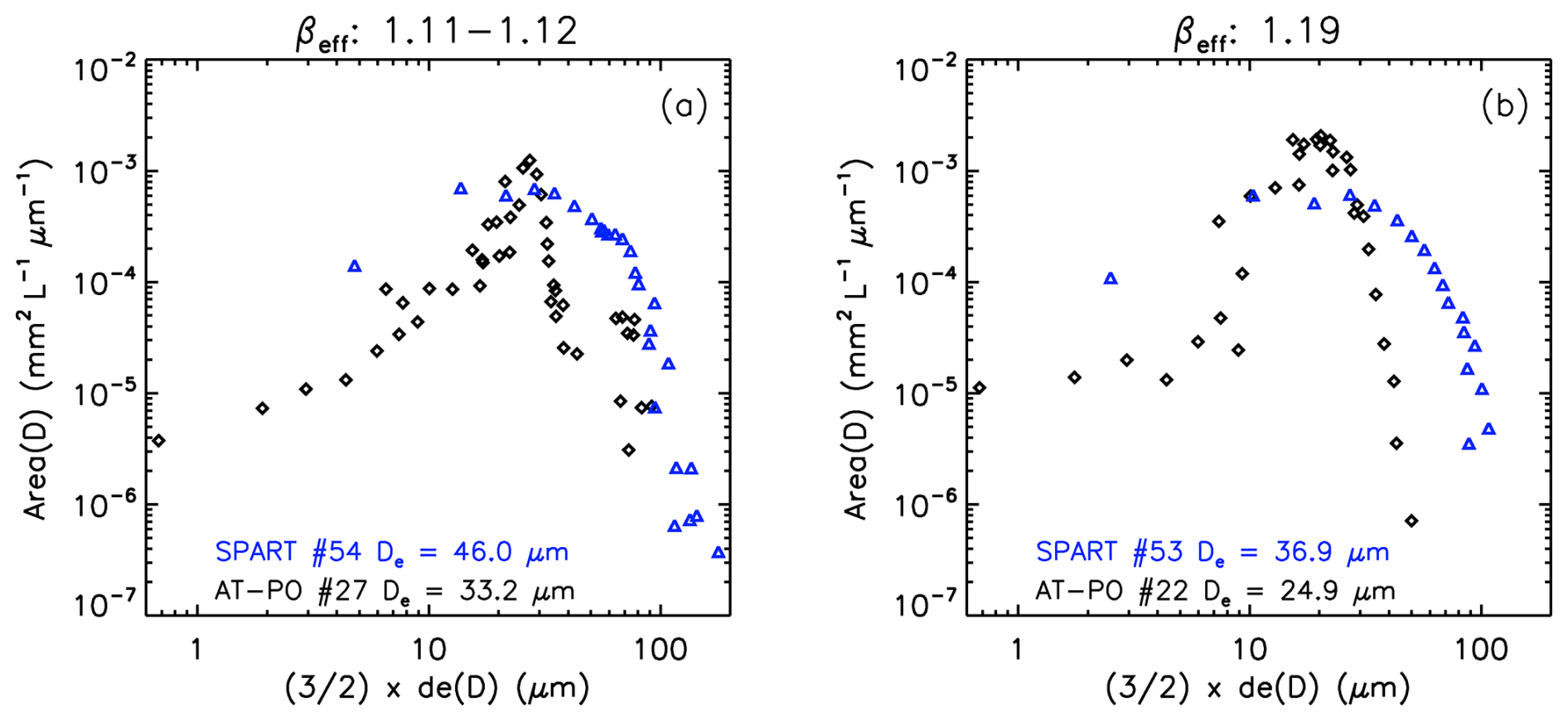
Figure 15 Comparisons of area PSDs from the ATTREX-POSIDON (black) and SPARTICUS (blue) campaigns having very similar β_eff values but considerably different D_e values, illustrating how differences in PSD shape between the two field campaigns can yield different D_e–β_eff relationships.

Note that X, which is sampled from aircraft (i.e., calculated from the sampled PSD), can be sampled at any level in the cloud, and from this sampled PSD, β_eff is also calculated using MADA as described in Sect. 2.3 of M2018, and Eqs. (4) and (5) from M2018. When X= $\mathrm{1}/Q_{\mathrm{abs}}$ (12 µm), the same is true but in this case X is calculated more like β_eff is calculated; β_eff can be viewed as a radiative characterization or microphysical index of the PSD. Despite large environmental differences among samples, the X–β_eff relationships obtained are relatively tight (i.e., dispersion is not large). This enables them to be used whereby a given point on these X–β_eff relationships represents a cloud layer of arbitrary thickness where β_eff is related to the PSD. The retrieval then matches the β_eff from these in situ X–β_eff relationships with the IIR retrieved β_eff to obtain retrieved X. Since the IIR retrieved β_eff corresponds to the extinction-weighted PSD for the cloud layer, retrieved X corresponds to this extinction-weighted PSD.

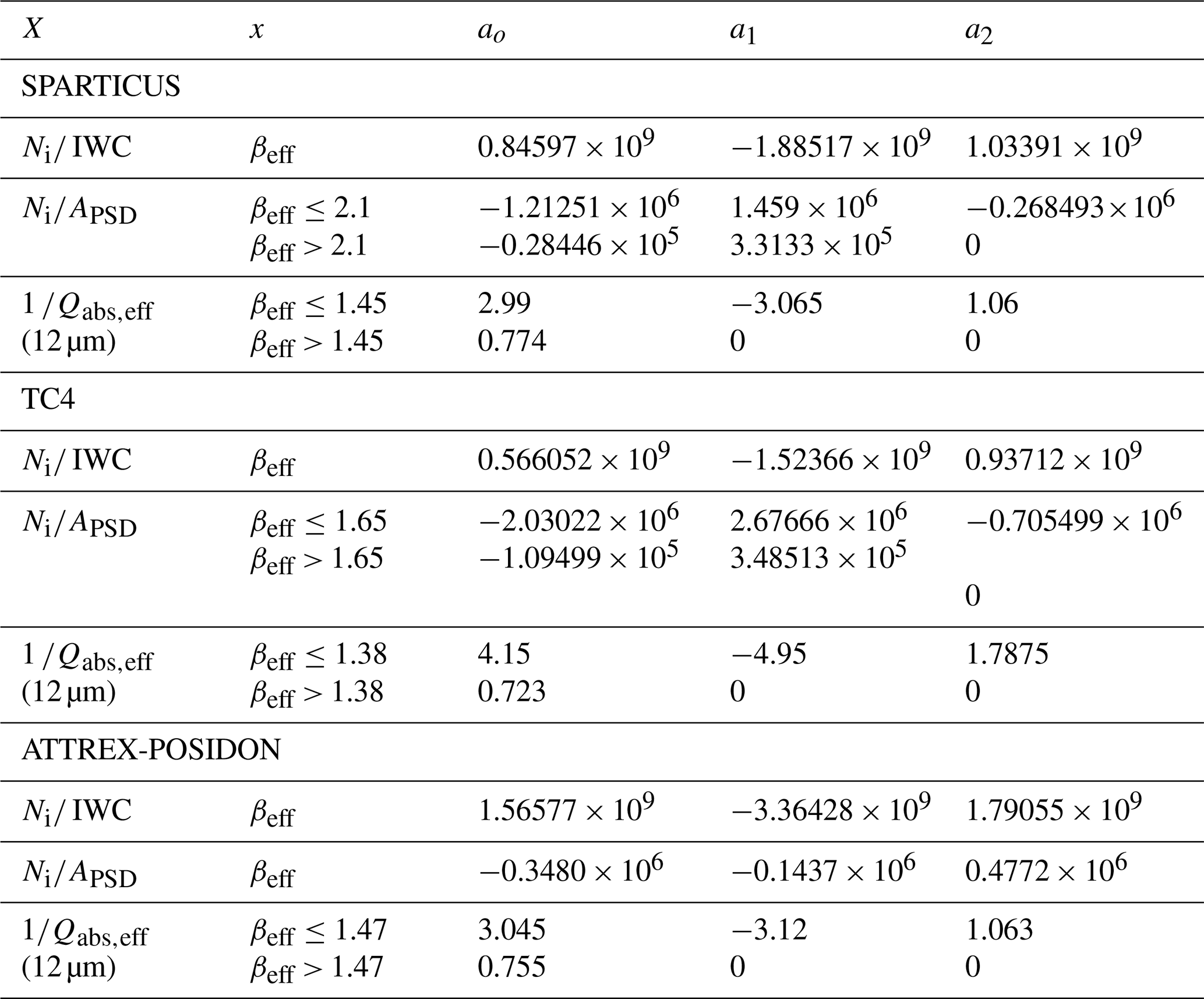
A plot similar to Fig. 14 but showing the curve fits only is included in the Supplement to this article (Fig. S1) and the coefficients used to produce these curves are listed in Table 3, where β_eff is the independent variable and the retrieved microphysical ratio is the dependent “X” variable. Sometimes a linear extrapolation had to be defined to extend the validity of the formulation over the full range of β_eff. These X–β_eff relationships in Table 3 are only valid when β_eff<10 (and are evaluated at β_eff= 10 if β_eff > 10). In practice, β_eff almost never exceeds 10 and rarely exceeds 2.

Table 3 Regression curve variables and coefficients for polynomials of the form $X=a_{\mathrm{0}}+a_{\mathrm{1}}\times +a_{\mathrm{2}}{x}^{\mathrm{2}}$ used in the CALIPSO retrieval. Units for $N_{\mathrm{i}}/$ IWC and $N/A_{\mathrm{PSD}}$ are in g⁻¹ and cm⁻², respectively.

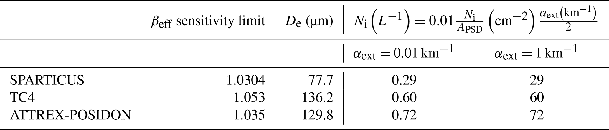
As noted in M2018, our retrieval of N_i and D_e is the most sensitive to β_eff when the PSD includes a large proportion of small ice crystals and β_eff is relatively large. The vertical dashed lines in Fig. 14 indicate the β_eff sensitivity limit for each field campaign dataset, which are listed in Table 4. If the retrieved β_eff lies below this value, the retrieved quantity in the X-column of Table 3 is evaluated at the β_eff sensitivity limit. Since D_e is essentially a product of two of these ratios, it is constant at the sensitivity limit, as shown in Table 4. However, when the retrieved property has an additional dependence on α_ext and therefore τ_abs (12.05 µm), that property is not a constant at the sensitivity limit since τ_abs (12.05 µm) is not subject to this limit. This is illustrated in Table 4, where the N_i retrieval equation is expressed in terms of the extinction coefficient for visible light α_ext. Two values of α_ext are given that bracket the α_ext range commonly found in cirrus, and corresponding N_i values are given for each α_ext and β_eff sensitivity limit, where $N_{\mathrm{i}}/A_{\mathrm{PSD}}$ is evaluated at the sensitivity limit for each campaign.

Table 4 Maximum retrieved D_e (µm) and minimum retrieved N_i (L⁻¹) at β_eff sensitivity limit.

3.3 Strategy for a global retrieval scheme

The X–β_eff relationships from the three field campaigns shown in Fig. 14 are overall consistent, but they exhibit differences. The D_e–β_eff relationship for TC4 differs significantly from that of the ATTREX-POSIDON campaigns, even though these three campaigns were conducted in the tropics, and they both differ from the SPARTICUS relationship obtained at mid-latitudes. For a given β_eff larger than 1.05, ATTREX-POSIDON yields the smallest D_e and SPARTICUS the largest one. By expressing PSDs in terms of d_e (effective photon path) as described in Sect. 2.4.1, Fig. 15 shows that TTL PSDs differ substantially from SPARTICUS PSDs over a narrow range of β_eff (i.e., β_eff is approximately constant). Since β_eff is essentially the ratio of two absorption coefficients involving the integration of PSD area, integrals of PSD area are shown. Each panel in Fig. 15 shows a SPARTICUS PSD and a PSD taken from either the ATTREX or POSIDON campaign, having similar β_eff values. In the bottom are the corresponding D_e values. It is seen that over a very narrow range of β_eff, D_e changes considerably (along with PSD shape), suggesting that the D_e–β_eff relationship is subject to changes in PSD shape. The number of TC4 PSDs were much less than for SPARTICUS, precluding the pairing of PSDs of similar β_eff. Nonetheless, it appears likely that PSD shape differences may be responsible for the different D_e–β_eff relationships regarding the anvil cirrus sampled during TC4 and the TTL cirrus sampled during ATTREX-POSIDON.

Supporting evidence relating to differences between anvil and TTL cirrus is found in Gasparini et al. (2018), which contrasted in situ cirrus dominating at $T<-\mathrm{55}$ °C (including TTL cirrus) with liquid origin cirrus dominating when −55 °C $<T<-\mathrm{40}$ °C, where the latter are either anvil cirrus formed from deep convection or are glaciated mixed phase clouds. Consistent with Gasparini et al. (2018), Heymsfield et al. (2014) found a D_e discontinuity in cirrus clouds in the tropics and at the top of mid-latitude clouds between ∼ −60 and −65 °C, with much smaller D_e at these lower temperatures (their Fig. 11).

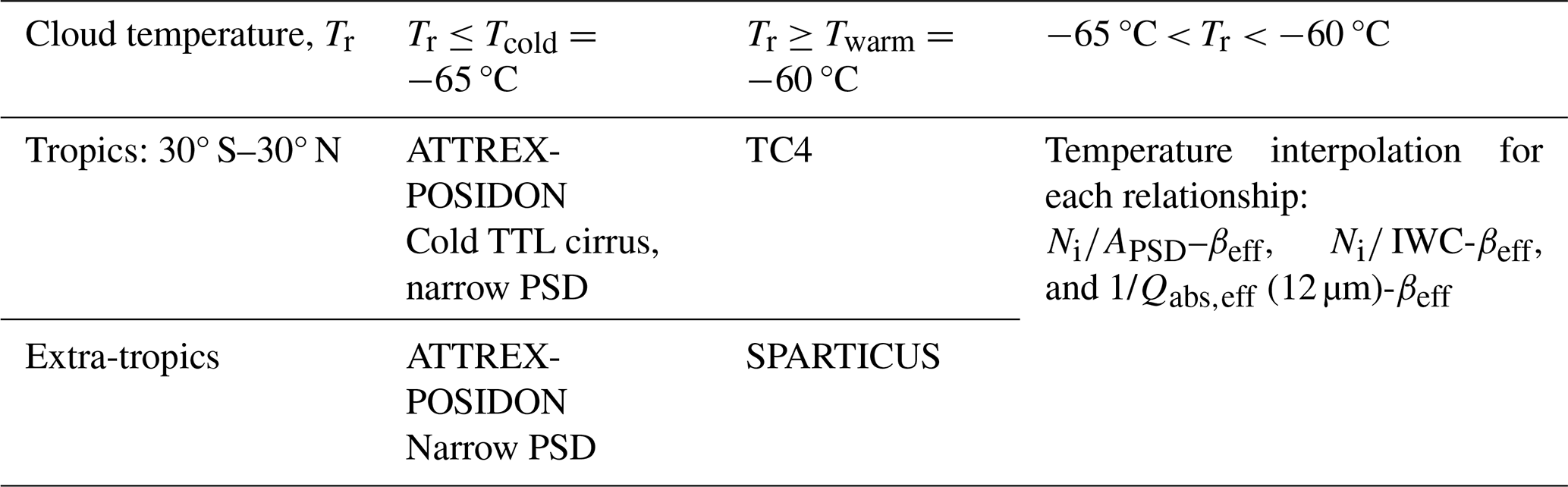
To accommodate these findings, we developed a latitude- and temperature-dependent scheme for our retrieval as described in Table 5. That is, for clouds having radiative temperature $T_{\mathrm{r}}<-$65 °C, the ATTREX-POSIDON D_e–β_eff relationship was used at any latitude. When $T_{\mathrm{r}}>-$60 °C, the TC4 D_e–β_eff relationship was used in the tropics (30° S–30° N) and the SPARTICUS D_e–β_eff relationship was used outside the tropics. Between −60 and −65 °C, a temperature interpolation between the two relevant formulations was implemented. The same practice applies to the other X–β_eff relationships as listed in Table 3. This temperature dependence mostly affects the tropics as shown in Fig. 16, featuring seasonal maps of the fraction of IIR pixels with cirrus clouds having $T_{\mathrm{r}}<-\mathrm{65}$ °C relative to all pixels with cirrus clouds (where cirrus clouds are defined as having T_r≤235 K). These fractions are for $\mathrm{0.01}<\mathit{\tau }<\sim$ 3 sampled only over oceans. This fraction was evaluated over both land and ocean using ∼ $\mathrm{0.3}<\mathit{\tau }<\sim$ 3 in the Supplement (Fig. S2) where it is shown that in the tropics, the fraction over land is comparable to that over the tropical western Pacific. Over the tropics, this fraction can easily exceed 60 % or 70 %, while outside the tropics, this fraction is generally <5 %, with exceptions over the Antarctic (JJA and SON) and over Greenland (DJF) as shown in the Supplement.

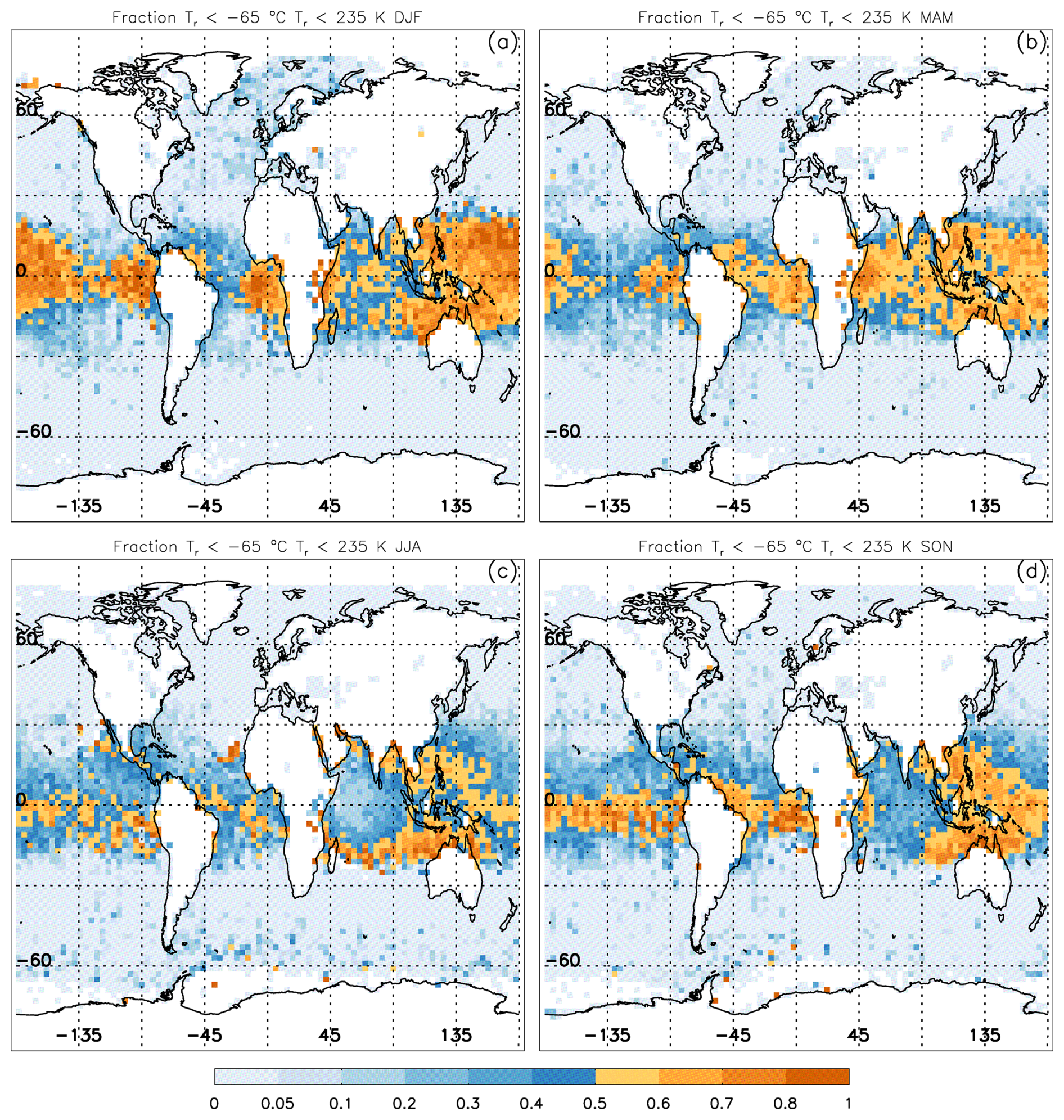
Figure 16 Seasonal maps of the fraction of cirrus cloud pixels (T_r≤ 235 K) having $T_{\mathrm{r}}<-\mathrm{65}$ °C (208 K) over oceans only, where ∼ 0.01 < τ < ∼ 3. This is the fraction of cirrus clouds for which the ATTREX-POSIDON formulation is used in this retrieval. The four panels are for (a) December–January–February (DJF), (b) March–April–May (MAM), (c) June–July–August (JJA), and (d) September–October–November (SON) during 2008, 2010, 2012 and 2013.

Table 5 Combination of the empirical relationships from the various campaigns. The T_cold and T_warm temperature limits were chosen based on the sampled temperatures during the respective campaigns.

The X–β_eff relationships listed in Table 3 together with the combination strategy listed in Table 5 can be used to reproduce the findings shown in Sect. 4 and in Part 2 of this study.

3.4 Retrieval uncertainties

Uncertainties in retrieved β_eff, noted Δβ_eff, translate into uncertainties in $N_{\mathrm{i}}/A_{\mathrm{PSD}}$, $N_{\mathrm{i}}/$ IWC, $\mathrm{1}/Q_{\mathrm{abs},\mathrm{eff}}$ (12 µm) and ultimately D_e. While Δβ_eff increases as optical depth decreases, the resulting uncertainty in X, noted ΔX, depends also on the $\partial X/\partial {\mathit{\beta }}_{\mathrm{eff}}$ slope of the X–β_eff relationships at retrieved β_eff. An additional contribution to the uncertainty in N_i, IWC and α_ext is the uncertainty in τ_abs (12 µm). The uncertainties in τ_abs (12 µm) and β_eff are estimated following the same rationale as in M2018. Details are given in Appendix B which includes the equations used to estimate the uncertainties in N_i, D_e, IWC, α_ext and R_v. Note that additional uncertainties in the X–β_eff relationships are difficult to estimate and are not included in this assessment. We see in the following section that relative uncertainties in N_i typically exceed 100 % when $\mathrm{0.01}<\mathit{\tau }<\sim$ 3. These large random uncertainties of individual retrievals can be mitigated by accumulating many samples. Median values of an ensemble of retrievals should not be too affected by the samples having β_eff smaller than the sensitivity limit for which $N_{\mathrm{i}}/A_{\mathrm{PSD}}$, $N_{\mathrm{i}}/$ IWC, $\mathrm{1}/Q_{\mathrm{abs},\mathrm{eff}}$ (12 µm) and ultimately D_e are set to constant values.

3.5 Comparison with previous work

For comparison with the previous work (M2018), Fig. 17a shows the $N_{\mathrm{i}}/{\mathit{\alpha }}_{\mathrm{abs}}$ ratio from the ATTREX-POSIDON (black), SPARTICUS (navy blue), and TC4 (red) relationships developed in this study vs. the $N_{\mathrm{i}}/{\mathit{\alpha }}_{\mathrm{abs}}$ ratio from SPARTICUS N(D)₁ unmodified established in M2018, which, out of the four formulations examined in M2018, yielded the largest N_i values (Fig. 5 in M2018). Also shown in Fig. 17a is TC4 N(D)₁= 0 from M2018 (dashed orange) which yielded the lowest N_i values. We see that N_i from this study is approximately half N_i from M2018 SPARTICUS unmodified for both SPARTICUS and TC4 which are similar to M2018 N(D)₁= 0, while the ATTREX-POSIDON value is a half to two thirds. Panel (b) in Fig. 17 compares the D_e retrievals.

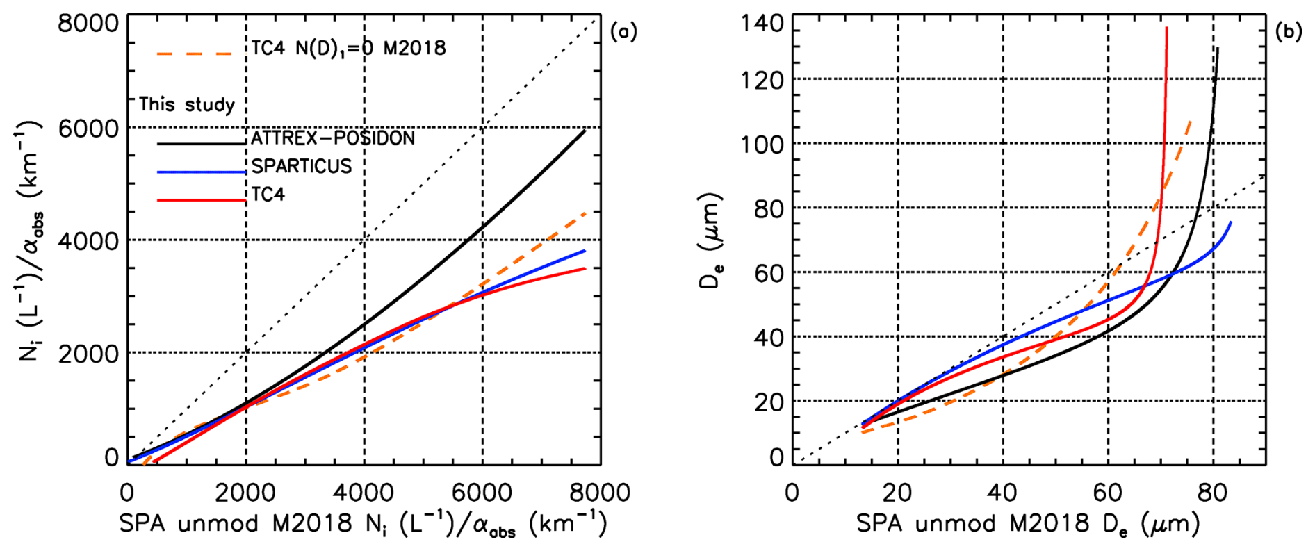
Figure 17 Comparison of (a) N_i and (b) D_e retrievals in this study (black: ATTREX-POSIDON, navy blue: SPARTICUS, red: TC4) and from TC4 N(D)₁= 0 in M2018 (dashed orange) with retrievals from SPARTICUS N(D)₁ unmodified in M2018.

4 Testing of the retrieval

Since this CALIPSO-IIR retrieval was developed from cirrus cloud field campaign measurements, we compared the satellite retrievals of N_i, D_e, IWC and α_ext during the period of the field campaigns over their respective regions with these same properties that were measured in situ during the field campaigns. In this section, the retrieval is tested against aircraft measurements from the ATTREX and POSIDON field campaigns for the tropics (together ATPO) and against SPARTICUS aircraft measurements for the midlatitudes. In addition, the Krämer et al. (2020) global climatology of cirrus cloud properties, based on numerous cirrus cloud field campaigns, is compared against the corresponding properties from this retrieval.

4.1 Comparisons with ATTREX and POSIDON PSD data

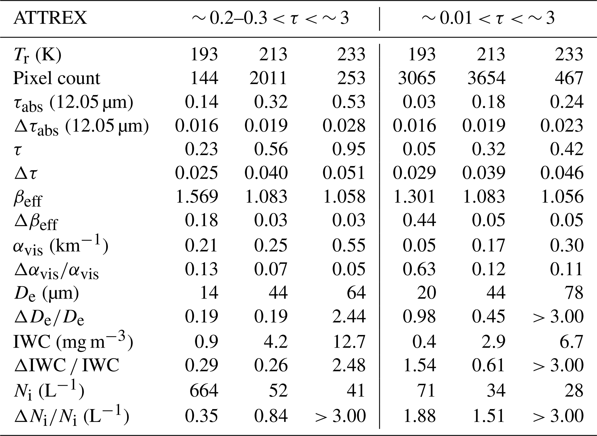
Since cirrus clouds sampled during these field campaigns were over ocean, their aircraft-measured properties can be compared against corresponding retrieved properties for cirrus having ∼ $\mathrm{0.01}<\mathit{\tau }<\sim$ 3, as shown for ATTREX in Fig. 18 and for POSIDON in Fig. 19. These retrievals were confined to the field campaign domain (in the tropical western Pacific) and to the campaign sampling period (February–March 2014 for ATTREX and October 2016 for POSIDON). The retrieval sample density is given by the color bar while the black diamonds indicate the aircraft in situ PSD measurements for a given property. The blue dashed curves in the D_e plots indicates the fraction of cirrus clouds for which D_e could be “reliably” retrieved (i.e., β_eff>β_eff sensitivity limit); D_e retrievals for which β_eff<β_eff sensitivity limit comprise the high sample densities between 130 and 136 µm. As PSDs broaden at higher temperatures, D_e increases and the β_eff<β_eff sensitivity limit occurs more often, which is evident from POSIDON in situ D_e and the blue dashed curve. Overall, the ATTREX and POSIDON retrievals appear consistent with the corresponding in situ values. Similar comparisons for optically thicker cirrus where ∼ $\mathrm{0.3}<\mathit{\tau }<\sim$ 3 are given in the Supplement (Figs. S3 and S4). Table 6 lists median retrieved properties and relative uncertainty estimates for ATTREX for cirrus having ∼ 0.2–$\mathrm{0.3}<\mathit{\tau }<\sim$ 3 (left) and ∼ $\mathrm{0.01}<\mathit{\tau }<\sim$ 3 (right). A similar table for the POSIDON campaign is shown in the Supplement (Table S1). In Table 6, median Δβ_eff ranges from 0.03 to 0.44 where median τ= 0.05 at T_r= 193 K, $\mathrm{\Delta }{N}_{\mathrm{i}}/N_{\mathrm{i}}=$ 1.88 and $\mathrm{\Delta }{D}_{\mathrm{e}}/D_{\mathrm{e}}=$ 0.98. The smallest median $\mathrm{\Delta }{N}_{\mathrm{i}}/N_{\mathrm{i}}$ is 0.35 at T_r= 193 K when only the thicker clouds are sampled and median τ is somewhat small (0.23), but this is compensated for by the fact that β_eff= 1.57 where the sensitivity of the technique is very favorable. In contrast, median β_eff is 1.056–1.058 at 233 K, where the sensitivity of the technique is less favorable, which explains the occurrence of relative uncertainties larger than 2.4 despite the small Δβ_eff= 0.03.

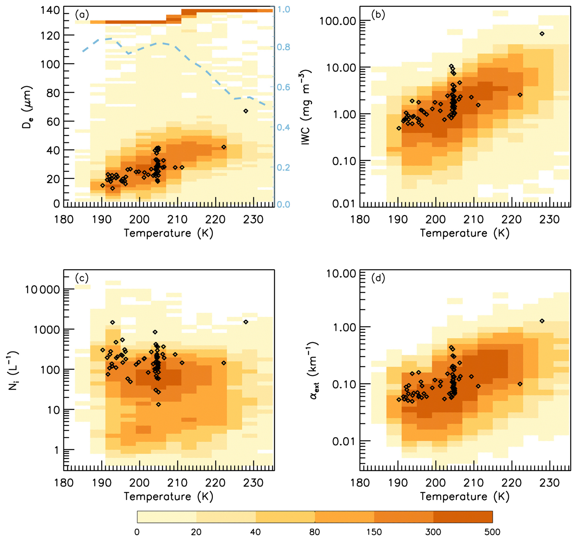
Figure 18 Pixel sampling densities (given by the color bar) for retrievals of (a) D_e, (b) IWC, (c) N_i, and (d) α_ext taken during the period of the ATTREX field campaign (February–March 2014) over the ATTREX domain (0–20° N and 130–160° E) where ∼ 0.01 < τ < ∼ 3. Black diamonds indicate corresponding aircraft PSD measurements of these properties. The right-hand vertical axis of the D_e plot indicates the fraction of cirrus clouds sampled having β_eff greater than the β_eff sensitivity limit given by the blue dashed curve while the high sample densities having D_e between 130 µm and 136 µm are from samples having β_eff lower than the β_eff sensitivity limit (i.e., non-quantifiable D_e). The change in D_e from 130 to 136 is due to the temperature interpolation (ATPO to TC4).

Again, these uncertainty estimates characterize random uncertainties of individual retrievals and are reduced for statistical analyses involving a large number of samples.

Table 6 Median values and estimated uncertainties of various retrieved properties at 193, 213, and 233 K for ∼ 0.2–0.3 < $\mathit{\tau }<\sim$ 3 (left) and ∼ 0.01 $<\mathit{\tau }<\sim$ 3 (right) during the ATTREX campaign.

4.2 Comparisons with SPARTICUS PSD data

As mentioned, N(D)₁ of the SPARTICUS PSD data was divided by 10.4 to correct N(D)₁ based on a comparison of N(D)₁ with corresponding FCDP values from the POSIDON campaign. These corrected SPARTICUS PSDs are used in this section to compare in situ cirrus cloud properties with corresponding retrieved values. As with the ATTREX and POSIDON campaigns, these retrievals are from the SPARTICUS domain (31–42° N and 90–103° W) during the campaign measurement period (January to April 2010). Since these retrievals are over land, they were restricted to the thicker cirrus where $\sim \mathrm{0.3}<\mathit{\tau }<\sim \mathrm{3}$. These comparisons are shown in Fig. 20. As before, the blue dashed curve in panel (a) indicates the fraction of D_e retrievals having β_eff > the β_eff sensitivity limit which corresponds to D_e≈ 78 µm (shown by the narrow band of high pixel sampling densities). At the highest cirrus temperatures (T_r), in situ D_e tends to be higher than retrieved D_e (where β_eff > the β_eff sensitivity limit). This may be partly due to aircraft sampling of relatively thick cirrus clouds below the mid-cloud level (i.e., at higher temperatures) where PSDs are broader (with larger D_e) due to longer ice particle growth times through vapor diffusion and aggregation. In contrast, retrieved D_e characterizes a layer and might reflect the presence of smaller crystals above the aircraft flight level. Similar reasons may explain why in situ IWCs tend to be higher than retrieved IWCs at higher T_r. Overall, the retrievals in Fig. 20 exhibit reasonable agreement with SPARTICUS in situ measurements, similar to the ATTREX and POSIDON comparisons.

Figure 19 Same as Fig. 18 but for the POSIDON field campaign in October 2016.

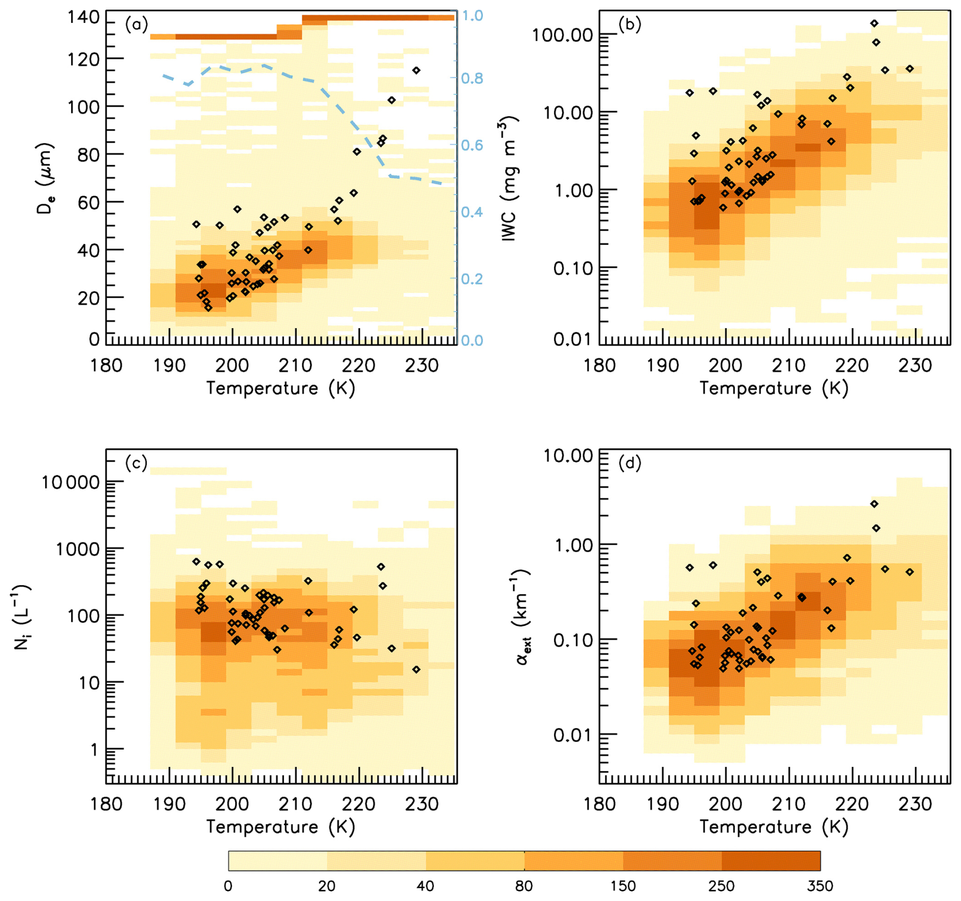
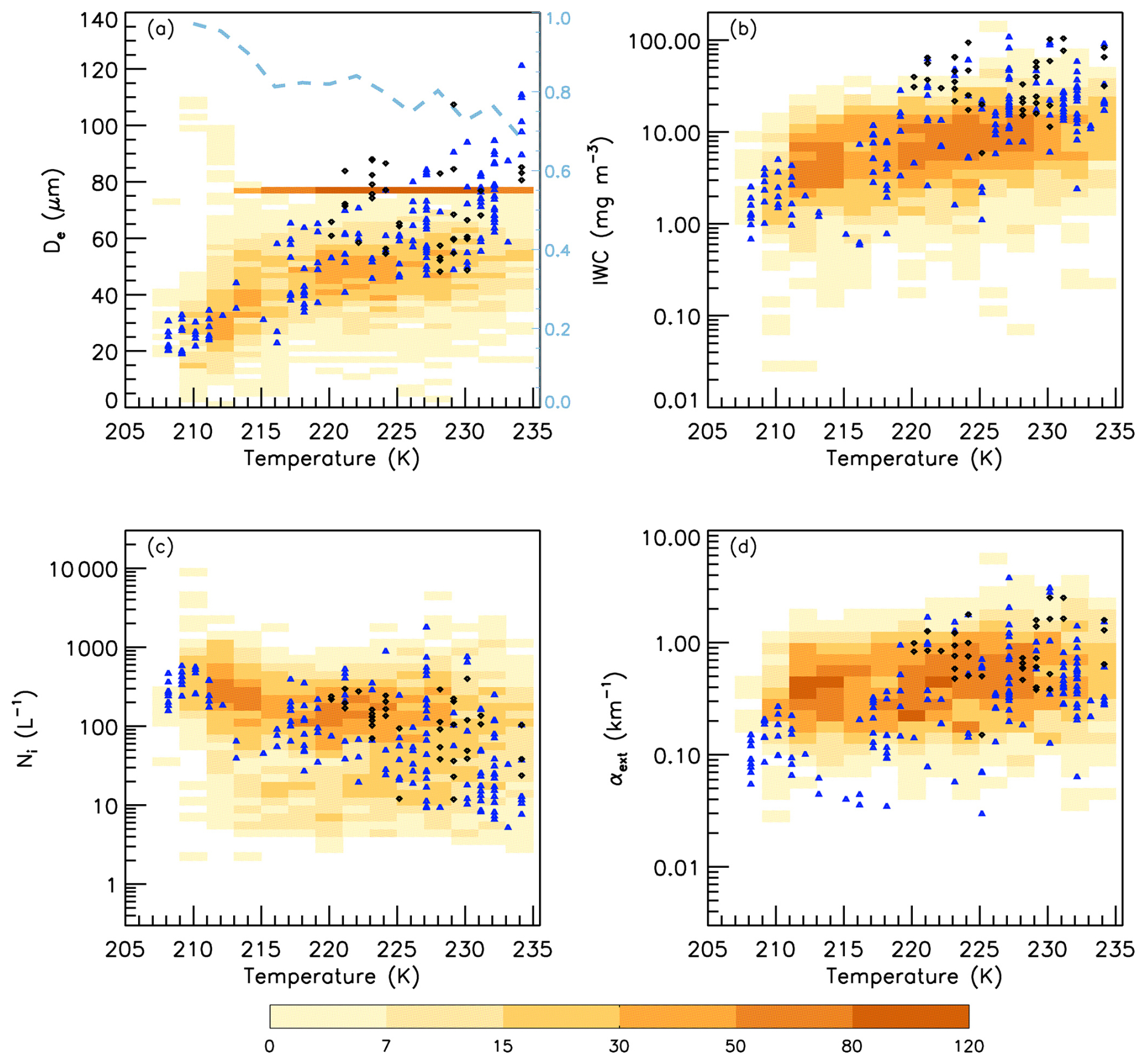
Figure 20 Pixel sampling densities (given by the color bar) for retrievals of (a) D_e, (b) IWC, (c) N_i, and (d) α_ext taken during the period of the SPARTICUS field campaign (January to April 2010) over the SPARTICUS domain (31–42° N; 90–103° W) where ∼ 0.3 < τ < ∼ 3. Black and blue symbols indicate corresponding aircraft PSD measurements of these properties for anvil and synoptic cirrus, respectively. The right-hand vertical axis of the D_e plot indicates the fraction of cirrus clouds sampled having β_eff greater than the β_eff sensitivity limit given by the blue dashed curve while the high sample densities having D_e ∼ 78 µm are from samples having β_eff lower than the β_eff sensitivity limit (i.e., non-quantifiable D_e).

The difficulty to directly compare IIR layer retrievals with aircraft in situ data is illustrated in the SPARTICUS case study shown in Fig. 21 for 30 March 2010. Following the CALIPSO track, the Learjet flew northwards (leg 1, triangles) with measurements at 11 km altitude 7 to 3 min before the CALIPSO overpass and then southwards (leg 2, diamonds) with measurements at 11.6 km altitude 6.5 to 8 min after. CALIPSO detected a single layer cirrus of top altitude near 12.6 km. The colors in panel (a) represent the altitude-dependent CALIOP extinction profiles scaled to IIR τ. The colors inside the triangles and diamonds indicate the PSD extinctions larger than 0.01 km⁻¹ after averaging over a 30 s period. At the top of panel (a) is IIR cloud layer α_ext, which was derived from τ and Δz_eq shown in panel (b). As discussed in Sect. 2.2.5, Δz_eq represents the portion of a layer contributing the most to the cloud emissivity. The solid black line in panel (a) is the radiative altitude corresponding to T_r, which to a first approximation corresponds to the mid-cloud altitude (see Fig. 7). IIR D_e in red in panel (c) (with vertical bars indicating D_e ± ΔD_e) is lower than the in situ values, which is explained by the fact that both flight legs were below the radiative altitude. That is, in the lower half of an ice cloud, mean ice particle size tends to be larger and N_i lower relative to the upper half due to diffusional growth and aggregation (e.g., Mitchell, 1988, 1994; Field and Heymsfield, 2003). Only a lower portion of the cloud was detected by the CloudSat radar (shown by the stars) between latitudes 36.5 and 36.78°. IIR D_e is the smallest (around 20 µm) south of 36.5° and north of 36.78° where there is no radar detection, indicating crystals smaller than about 40 µm. Moreover, the absence of radar detection outside this CloudSat domain (defined by the stars) indicates ice particles smaller than ∼ 40 µm, revealing a vertical gradient in ice particle size. Regarding N_i (panel (d) showing N_i ± ΔN_i), the large IIR N_i values in red between 300 and 850 L⁻¹ are explained by higher N_i near cloud top. Regarding uncertainties, ΔN_i is overall equal to about 80 L⁻¹ and its noticeable increase up to 300 L⁻¹ in the northernmost part of the cloud is due to the decrease of τ. The same observation applies to ΔD_e which is between 3 and 11 µm. To summarize, while the vertically resolved extinction retrievals exhibit reasonable agreement with the in situ extinction measurements, the bulk cloud layer retrievals often do not exhibit similar agreement, and this appears to be due to vertical gradients in D_e and N_i and aircraft sampling location. This case study has been classified as ridge crest cirrus which have higher N_i than the other cirrus cloud classes described in Muhlbauer et al. (2014). In this regard, the retrievals here are consistent with this category of cirrus cloud.

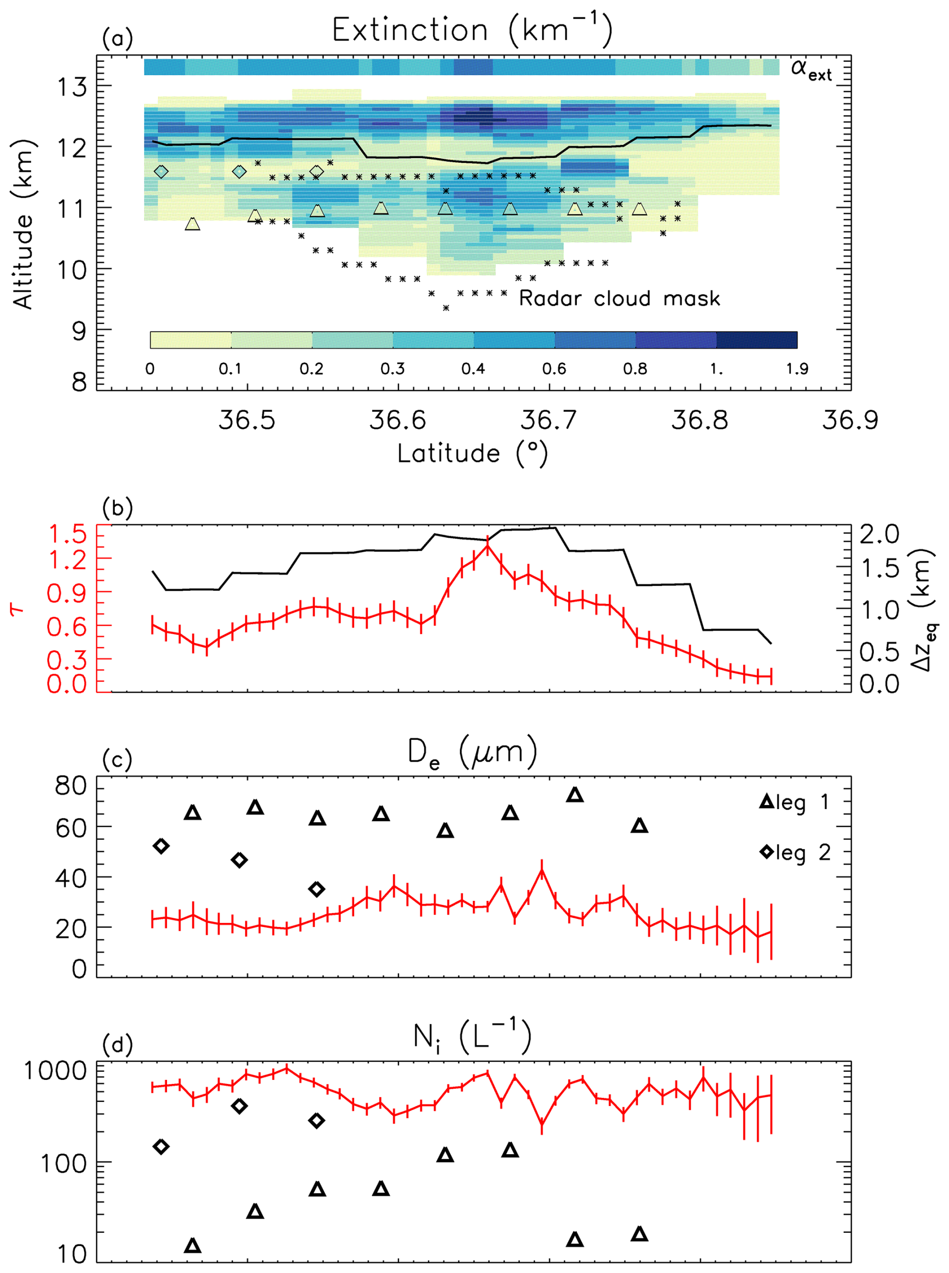
Figure 21 Comparison of IIR retrievals and in situ observations on 30 March 2010 during the SPARTICUS field campaign (CALIPSO granule 2010-03-30T19-27-25ZD). (a) extinction profile derived from the CALIOP lidar, IIR layer α_ext, and PSD extinctions in leg 1 (triangles) and leg 2 (diamonds). The solid black line in panel (a) is the radiative altitude corresponding to T_r. The stars denote the boundaries of the CloudSat radar GEOPROF cloud mask, and the color bar at the bottom gives α_ext values; (b) IIR τ (red) and Δz_eq (black, right-hand axis); (c) IIR (red) and in situ (triangles and diamonds) D_e; (d) same as (c) but for N_i. The vertical bars in red in panels (b)–(d) represent the IIR estimated uncertainties.

4.3 Comparisons with a global cirrus cloud property climatology

A recent study by Krämer et al. (2020) has expanded the in situ cirrus cloud property database described in Krämer et al. (2009) by a factor of 5 to 10 (depending on cloud property). Here we compare the temperature dependence of R_v, N_i and IWC from the CALIPSO-IIR retrievals and from the Krämer et al. (2020) climatology. Since the aircraft measurements used in Krämer et al. (2020) often did not allow D_e to be calculated (and thus D_e was not reported), we use R_v as a measure of ice particle size for comparison purposes since R_v is reported in Krämer et al. (2020). However, R_v and D_e are unique quantities where D_e cannot be calculated from R_v (and vice-versa). Since D_e partly determines a cloud's radiative properties, D_e and R_v are intercompared in Appendix C based on in situ data and for different PSD shape assumptions using a PSD model that assumes a simple gamma PSD distribution. While natural PSDs exhibit shapes more complex than these gamma PSDs, this modeling exercise suggests the relation between D_e and R_v depends on PSD shape.

Figure 3 in Krämer et al. (2020) shows that aircraft measurements are mostly between 20° S and 63° N. Thus, the IIR retrievals were averaged over oceans for 20° S–0°, 0°–30° N, and 30–63° N for 4 years (2008, 2010, 2012 and 2013). Since the Krämer et al. (2020) data have no seasonal dependence, IIR retrievals were averaged over all seasons. The results are shown in Fig. 22, where the IIR results, using T_r for the temperature, are in red for samples with τ > ∼ 0.3 and in blue using τ > ∼ 0.01. In situ data (black curves) in panels (a) and (c) are the climatological values. In panel (d) showing IWC, the black curve is an estimate of median in situ IWC derived from median in situ R_v and median in situ N_i using Eq. (5). The retrieved values of R_v, N_i and IWC for τ>0.01 (blue curves) are generally within the ± 25 percentile range of corresponding in situ values.

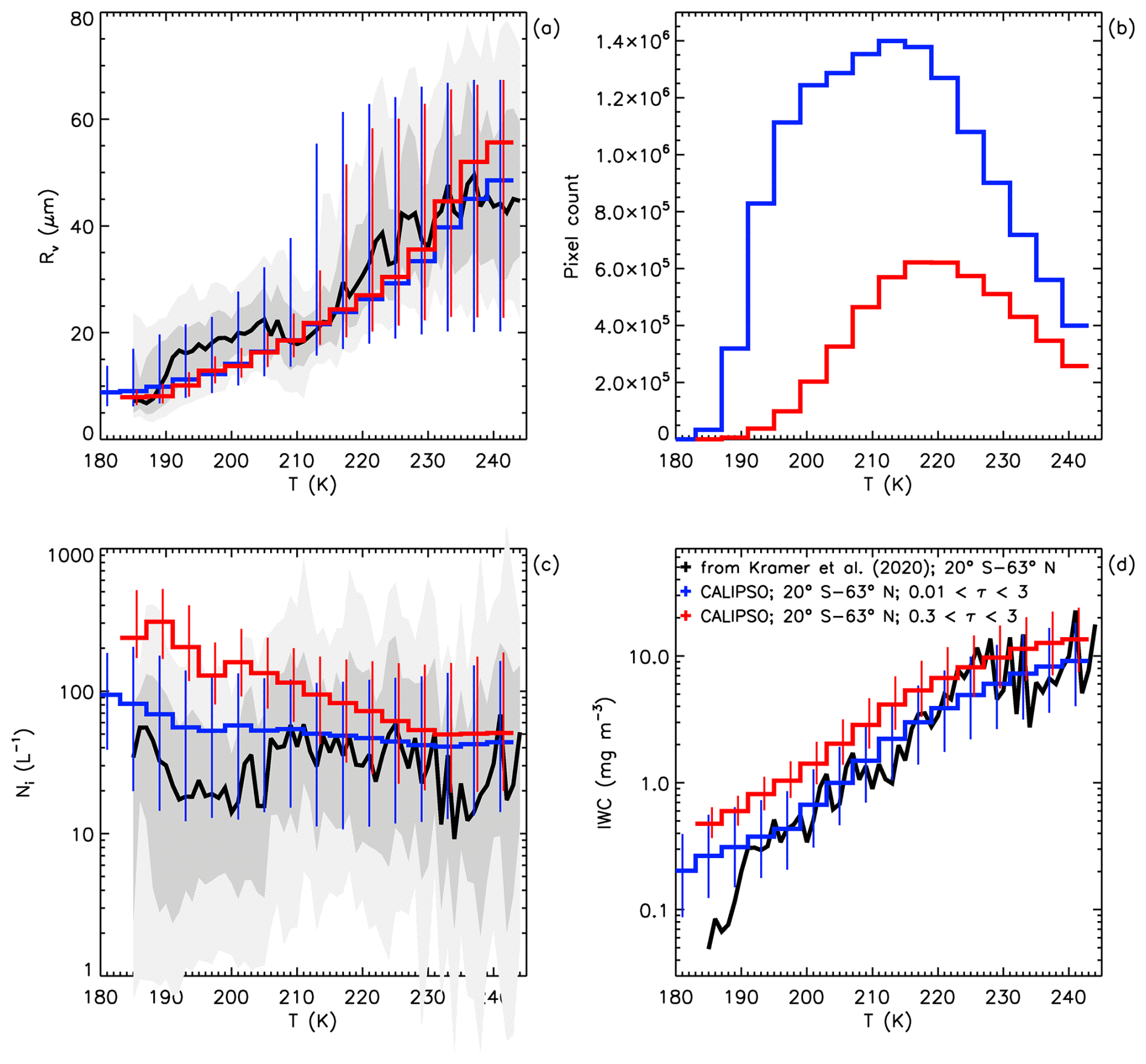
Figure 22 Temperature dependence of median values of (a) R_v (µm), (c) N_i (L⁻¹), and (d) IWC (mg m⁻³) from the IIR retrievals (red: ∼ 0.3 < τ < ∼ 3; blue: ∼ 0.01 < τ < ∼ 3) and from the Krämer et al. (2020) in situ climatology (black curves). The vertical bars indicate the IIR 25th and 75th percentiles, except in panel (b) which shows the number of IIR sampled pixels. The light shade of gray in panels (a) and (c) is between the 10th and 90th percentiles and the superimposed darker shade of gray is between the 25th and 75th percentiles for the in situ data.

The large spread of IIR data when τ can be as low as ∼ 0.01 (blue) compared to τ > ∼ 0.3 (red) is due in part to larger random uncertainties in clouds having optical depth <0.3, which represent the majority of the samples at T<215 K (panel (b)). We note, however, that median R_v from the red and blue curves are similar, suggesting no systematic bias introduced by the retrievals at $\mathit{\tau }<\sim$ 0.3. IIR and in situ median R_v agree reasonably well at T > 210 K and below 190 K. IIR R_v increases steadily with temperature and can be lower than in situ R_v by up to 7 µm between 190 and 205 K.

Differences between the optically thicker (τ > 0.3, red) and thinner (τ > 0.01, blue) N_i and IWC retrievals may be due to differences in ice nucleation processes (i.e., het and hom) as described in Part 2, with hom occurring more often in the optically thicker cirrus clouds, promoting higher N_i and IWC. If true, it may be important during cirrus cloud field campaigns to attempt to characterize the cirrus in terms of τ to make in situ cloud property comparisons with cirrus cloud remote sensing and climate modeling results more meaningful. Fortunately, Krämer et al. (2020) contains a disclaimer stating, “Because of the dangerous nature of measurements under such conditions, the frequency of convective – and also orographic wave cirrus – is underrepresented in the entire in situ climatology”. And related to this, there is a statement about the higher in situ N_i in Krämer et al. (2009) resulting from flights in the “lee wave cirrus behind the Norwegian mountains”. Orographic gravity waves (OGWs) produce relatively high updrafts more conducive to hom and tend to produce optically thicker cirrus clouds with higher N_i that can be spatially extensive (M2018). The sparsity of OGW cirrus in situ sampling in Krämer et al. (2020) may help explain the tendency of IIR N_i being slightly higher than in situ N_i in Fig. 22.

The retrieved median N_i in Fig. 22 (blue curve) exhibit similar magnitudes as a function of temperature to those of the DARDAR N_i retrieval (Sourdeval et al., 2018), which are compared against the median N_i of the Krämer et al. climatology in Fig. 15 of Krämer et al. (2020). The main difference between the DARDAR N_i retrieval and this one is that median DARDAR N_i is higher for T<220 K, with DARDAR N_i ∼ 100 L⁻¹ for T<205 K.

5 Conclusions

This study has utilized the CALIPSO IIR and CALIOP lidar in new ways, resulting in new methods for retrieving N_i, D_e, IWC, IWP, α_ext and τ. The following improvements contributed to this CALIPSO retrieval:

1. By expanding the sampling range to include optically thinner cirrus clouds (0.01 < τ < 3) over oceans, the sampling has become more representative of all cirrus clouds over oceans. The sampling over land, snow and sea ice remains limited to thicker cirrus clouds having τ > 0.3 because of larger uncertainties in IIR absorption optical depth retrievals.

2. The retrieval of N_i has become more accurate by using the $N_{\mathrm{i}}/A_{\mathrm{PSD}}$ ratio, which is directly measured by aircraft probes.

3. The computation of in situ β_eff used in the X–β_eff relationships was improved using mass-dimension relationships that appear more realistic.

4. The retrieval of D_e has become more accurate by using the ratios $N_{\mathrm{i}}/A_{\mathrm{PSD}}$ and $N_{\mathrm{i}}/$ IWC, where IWC is estimated using the more realistic mass-dimension relationships.

5. Improvements in D_e accuracy transfer to improvements in IWC and IWP accuracy via Eqs. (6) and (9), respectively.

6. The relationship between D_e and β_eff was not unique, where PSDs having the same β_eff can have different D_e due to PSD shape differences between TTL cirrus and cirrus at higher temperatures. For this reason, separate X–β_eff relationships were developed for TTL and anvil (or synoptic) cirrus, with a temperature interpolation linking these two temperature regimes. This mostly affects the tropics where cirrus clouds are abundant in the TTL (see Fig. 16). The X–β_eff relationships for the SPARTICUS synoptic and the TC4 anvil cirrus yield similar N_i retrievals (see Fig. 17).

7. By comparing the FCDP and 2D-S probes in their overlap region, the first size bin of the 2D-S probe was corrected to a first approximation, resulting in improved X–β_eff relationships.

8. In general, the physical properties of cirrus clouds differ when comparing optically thicker ($\mathrm{0.3}<\mathit{\tau }<\mathrm{3}$) cirrus clouds with all cirrus clouds ($\mathrm{0.01}<\mathit{\tau }<\mathrm{3}$), where N_i and IWC are higher in the optically thicker cirrus clouds.

This study should be extended to more field campaigns, in particular at high latitude, to further investigate the variability in the X–β_eff relationships, which seems more important for D_e than for N_i. In view of point (8) (above), cirrus cloud field campaigns should indicate, if possible, the type of cirrus clouds being sampled, especially outside the tropics where OGW cloud cirrus (often having τ > 0.3) are common (M2018). A global/seasonal analysis of the frequency of occurrence of these OGW cirrus clouds, developed through satellite remote sensing, would also be useful for testing the representation of cirrus clouds in climate models, given their distinct optical properties.

Given the apparent dependence of N_i and IWC on τ, the agreement between the two remote sensing methods (DARDAR and CALIPSO) and the Krämer et al. (2020) climatology appears reasonable. That is, cirrus associated with strong updrafts (i.e., anvil cirrus near convection and OGW cirrus) are generally avoided during cirrus field campaigns for safety reasons (Krämer et al., 2020) and therefore may not be accurately represented by in situ sampling-based climatology. It may be possible that the high median DARDAR N_i (∼ 100 L⁻¹) for T<205 K (Krämer et al., 2020, Fig. 15) relative to in situ climatological N_i in Fig. 22 results from the DARDAR sampling of thick anvil cirrus near convection where hom affects N_i more profoundly. This CALIPSO retrieval does not sample such cirrus (i.e., τ > 3) and thus would retrieve a lower median climatological N_i. Nonetheless, tropical cirrus clouds having τ<3 are probably representative of tropical cirrus in terms of their areal coverage, which matters most for cloud radiative effects.

This CALIPSO retrieval provides layer properties based on layer β_eff and the IIR weighting function derived from the CALIOP extinction profiles at 532 nm. Future work could aim at estimating in-cloud vertical profiles of IWC, D_e, and N_i. This would require knowledge of the in-cloud variation of β_eff, which could be inferred from a priori assumptions regarding variations of D_e further constrained by co-located CloudSat radar observations when available.

The application of this CALIPSO retrieval for studying the physics of cirrus clouds is exemplified in Part 2 of this article. In particular, a method for estimating the fraction of cirrus clouds strongly affected by hom is presented as well as a new conceptual model for cirrus cloud formation and evolution.

Appendix A: Inter-channel optical depth differences

Both over land and over oceans, the solid lines in Figs. 3 and 4 tend to zero as IAB tends to zero, as expected. The median τ_abs12–10 differences are listed in Table A1. To estimate whether these differences are realistic, Table A1 also includes an approximate β_eff derived from the median τ_abs12–10 and median τ_abs (12.05 µm) listed in Table 1 as

$$\begin{array}{}\text{(A1)}& {\mathit{\beta }}_{\mathrm{eff}}\mathrm{proxy}={\displaystyle \frac{\mathrm{median}{\mathit{\tau }}_{\mathrm{abs}}\left(\mathrm{12.05}\mathrm{\mu }\mathrm{m}\right)}{\mathrm{median}{\mathit{\tau }}_{\mathrm{abs}}\left(\mathrm{12.05}\mathrm{\mu }\mathrm{m}\right)-\mathrm{median}{\mathit{\tau }}_{\mathrm{abs}}\mathrm{12}-\mathrm{10}}}.\end{array}$$

This approximate β_eff is the ratio of two very small optical depths (smaller than 0.01) and is therefore very sensitive to small inter-channel biases. It is as expected larger than 1, except at 0–30° N over land in DJF where it is only slightly smaller. We estimate that the upper range of realistic values for β_eff is ∼ 1.5–2, so that β_eff= 3.2 at 60–82° N over oceans in DJF is unambiguously overestimated. Decreasing τ_abs12–10 from 0.0029 to 0.0010 would bring β_eff to 1.3, suggesting a positive 12–10 inter-channel bias ≤0.002 at 60–82° N over oceans in DJF. Note that the impact of such an inter-channel bias decreases sharply as optical depth increases (Garnier et al., 2021a). For instance, at τ_abs (12.05 µm) = 0.05, corresponding to IAB ∼ 0.004 in Fig. 2, β_eff= 1.2 in Fig. 4 could correspond to true β_eff∼ 1.145, i.e., β_eff could be overestimated but less than 0.06. At τ_abs (12.05 µm) = 0.15, corresponding to IAB ∼ 0.01 in Fig. 2, β_eff= 1.15 in Fig. 4 could be overestimated by less than 0.02.

Table A1 Median IIR τ_abs (12.05 µm)–τ_abs (10.6 µm) (i.e., τ_abs12–10) at CALIOP IAB ∼ 7.6 × 10⁻⁴ sr⁻¹ using all retrievals (cf. solid lines in Figs. 3 and 4) and an approximation for β_eff (Eq. A1).

Appendix B: Retrieval uncertainty analysis

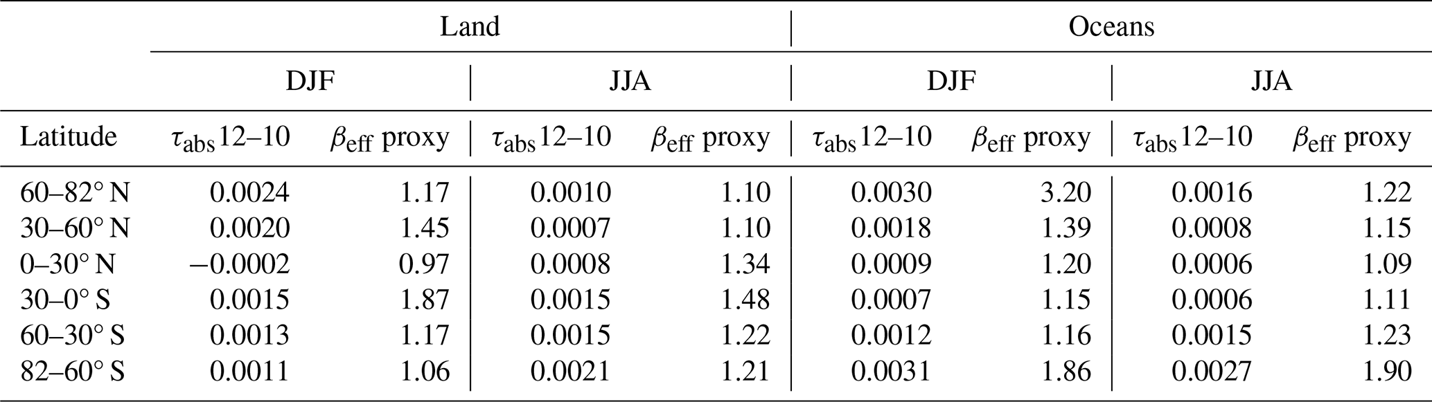
B1 Ice particle number concentration, N_i

The retrieval equation for the ice particle number concentration, N_i, is

$$\begin{array}{}\text{(B1)}& N_{\mathrm{i}}={\left[{\displaystyle \frac{N_{\mathrm{i}}}{A_{\mathrm{PSD}}}}\right]}_{{\mathit{\beta }}_{\mathrm{eff}}}{\displaystyle \frac{{\mathit{\tau }}_{\mathrm{abs}}\left(\mathrm{12.05}\mathrm{\mu }\mathrm{m}\right)}{{\left[Q_{\mathrm{abs},\mathrm{eff}}\left(\mathrm{12}\mathrm{\mu }\mathrm{m}\right)\right]}_{{\mathit{\beta }}_{\mathrm{eff}}}\mathrm{\Delta }{z}_{\mathrm{eq}}}}.\end{array}$$

The quantities $N_{\mathrm{i}}/A_{\mathrm{PSD}}$ and $\mathrm{1}/Q_{\mathrm{abs},\mathrm{eff}}$ (12 µm) are retrieved from β_eff using regression curves and the coefficients listed in Table 3. By writing x=β_eff, they are computed as

$$\begin{array}{}\text{(B2)}& \left({\displaystyle \frac{N_{\mathrm{i}}}{A_{\mathrm{PSD}}}}\right)\left({\mathrm{cm}}^{-\mathrm{2}}\right)={\sum }_{i=\mathrm{0}}^{i=\mathrm{2}}{b}_{\mathrm{i}}{x}^i\end{array}$$

and

$$\begin{array}{}\text{(B3)}& {\displaystyle \frac{\mathrm{1}}{Q_{\mathrm{abs},\mathrm{eff}}\left(\mathrm{12}\mathrm{\mu }\mathrm{m}\right)}}={\sum }_{i=\mathrm{0}}^{i=\mathrm{2}}{c}_{\mathrm{i}}{x}^i.\end{array}$$

Equation (B1) can be re-written as

$$\begin{array}{}\text{(B4)}& N_{\mathrm{i}}\left({\mathrm{L}}^{-\mathrm{1}}\right)=\mathrm{0.01}\times f\left(x\right)\left({\mathrm{cm}}^{-\mathrm{2}}\right)\times {\mathit{\alpha }}_{\mathrm{abs}}\left({\mathrm{km}}^{-\mathrm{1}}\right),\end{array}$$

with

$$\begin{array}{}\text{(B5)}& f\left(x\right)=\left({\sum }_{i=\mathrm{0}}^{i=\mathrm{2}}{b}_{\mathrm{i}}{x}^i\right)\left({\sum }_{i=\mathrm{0}}^{i=\mathrm{2}}{c}_{\mathrm{i}}{x}^i\right)\end{array}$$

and

$$\begin{array}{}\text{(B6)}& {\mathit{\alpha }}_{\mathrm{abs}}={\displaystyle \frac{{\mathit{\tau }}_{\mathrm{abs}}\left(\mathrm{12.05}\mathrm{\mu }\mathrm{m}\right)}{\mathrm{\Delta }{z}_{\mathrm{eq}}}}.\end{array}$$

Assuming a negligible error in ΔZ_eq, and writing τ_abs (12.05 µm) as τ₁₂ and τ_abs (10.6 µm) as τ₁₀ for more clarity, so that $x={\mathit{\tau }}_{\mathrm{12}}/{\mathit{\tau }}_{\mathrm{10}}$, the derivative of N_i can be written

$$\begin{array}{}\text{(B7)}& {\displaystyle \frac{\mathrm{d}{N}_{\mathrm{i}}}{N_{\mathrm{i}}}}={\displaystyle \frac{\mathrm{1}}{f}}{\displaystyle \frac{\partial f}{\partial x}}x\left({\displaystyle \frac{\mathrm{d}{\mathit{\tau }}_{\mathrm{12}}}{{\mathit{\tau }}_{\mathrm{12}}}}-{\displaystyle \frac{\mathrm{d}{\mathit{\tau }}_{\mathrm{10}}}{{\mathit{\tau }}_{\mathrm{10}}}}\right)+{\displaystyle \frac{\mathrm{d}{\mathit{\tau }}_{\mathrm{12}}}{{\mathit{\tau }}_{\mathrm{12}}}}.\end{array}$$

In Eq. (B7), the derivative of x=β_eff is

$$\begin{array}{}\text{(B8)}& \mathrm{d}x=\mathrm{d}{\mathit{\beta }}_{\mathrm{eff}}=x\left({\displaystyle \frac{\mathrm{d}{\mathit{\tau }}_{\mathrm{12}}}{{\mathit{\tau }}_{\mathrm{12}}}}-{\displaystyle \frac{\mathrm{d}{\mathit{\tau }}_{\mathrm{10}}}{{\mathit{\tau }}_{\mathrm{10}}}}\right).\end{array}$$

Errors in τ₁₂ and in τ₁₀ are computed by propagating errors in (i) the measured brightness temperatures T_m, (ii) the background brightness temperatures T_BG and (iii) the blackbody brightness temperatures T_BB (Garnier et al., 2015, 2021a, M2018). For each of the three temperature (T) components (T_BG, T_BB and T_m), $\frac{\partial \mathit{\tau }}{\partial T}$ in channels 12 and 10 is computed as

$$\begin{array}{}\text{(B9)}& {\displaystyle \frac{\partial \mathit{\tau }}{\partial T}}={\displaystyle \frac{\mathrm{1}}{\mathrm{1}-\mathit{\epsilon }}}{\displaystyle \frac{\partial \mathit{\epsilon }}{\partial \mathrm{T}}},\end{array}$$

where the effective emissivity in the channel, ε, and the three associated $\frac{\partial \mathit{\epsilon }}{\partial T}$ terms are reported in the IIR Version 4 product.

The uncertainties ΔT_m10 in T_m10 at 10.6 µm and ΔT_m12 in T_m12 at 12.05 µm are random errors set to 0.3 K, which are statistically independent (Garnier et al., 2015, 2021a). Because the same cloud temperature is used to compute τ₁₂ and τ₁₀, the uncertainty ΔT_BB in T_BB is the same at 10.6 and at 12.05 µm. A random error of ±2 K is estimated to include errors in the atmospheric model. Finally, it was shown in Garnier et al. (2021a) that the uncertainty ΔT_BG in T_BG can be considered identical in both channels; ΔT_BG is estimated to be 1 K over oceans and 3 K over land.

Finally, the relative uncertainty $\mathrm{\Delta }{N}_{\mathrm{i}}/N_{\mathrm{i}}$ is written as

$$\begin{array}{}\text{(B10)}& \begin{array}{rl}& {\left({\displaystyle \frac{\mathrm{\Delta }{N}_{\mathrm{i}}}{N_{\mathrm{i}}}}\right)}^{\mathrm{2}}=\\ & {\left[{\displaystyle \frac{\mathrm{1}}{f}}{\displaystyle \frac{\partial f}{\partial x}}x\left({\displaystyle \frac{\partial {\mathit{\tau }}_{\mathrm{12}}}{{\mathit{\tau }}_{\mathrm{12}}\partial T_{\mathrm{BG}}}}-{\displaystyle \frac{\partial {\mathit{\tau }}_{\mathrm{10}}}{{\mathit{\tau }}_{\mathrm{10}}\partial T_{\mathrm{BG}}}}\right)+{\displaystyle \frac{\partial {\mathit{\tau }}_{\mathrm{12}}}{{\mathit{\tau }}_{\mathrm{12}}\partial T_{\mathrm{BG}}}}\right]}^{\mathrm{2}}\\ & \mathrm{\Delta }{T}_{\mathrm{BG}}^{\mathrm{2}}+\left[{\displaystyle \frac{\mathrm{1}}{f}}{\displaystyle \frac{\partial f}{\partial x}}x\left({\displaystyle \frac{\partial {\mathit{\tau }}_{\mathrm{12}}}{{\mathit{\tau }}_{\mathrm{12}}\partial T_{\mathrm{BB}}}}-{\displaystyle \frac{\partial {\mathit{\tau }}_{\mathrm{10}}}{{\mathit{\tau }}_{\mathrm{10}}\partial T_{\mathrm{BB}}}}\right)\right.\\ & {\left.+{\displaystyle \frac{\partial {\mathit{\tau }}_{\mathrm{12}}}{{\mathit{\tau }}_{\mathrm{12}}\partial T_{\mathrm{BB}}}}\right]}^{\mathrm{2}}\mathrm{\Delta }{T}_{\mathrm{BB}}^{\mathrm{2}}+{\left[\left({\displaystyle \frac{\mathrm{1}}{f}}{\displaystyle \frac{\partial f}{\partial x}}x+\mathrm{1}\right){\displaystyle \frac{\partial {\mathit{\tau }}_{\mathrm{12}}}{{\mathit{\tau }}_{\mathrm{12}}\partial T_{\mathrm{m}\mathrm{12}}}}\right]}^{\mathrm{2}}\\ & \mathrm{\Delta }{T}_{\mathrm{m}\mathrm{12}}^{\mathrm{2}}+{\left[\left({\displaystyle \frac{\mathrm{1}}{f}}{\displaystyle \frac{\partial f}{\partial x}}x\right){\displaystyle \frac{\partial {\mathit{\tau }}_{\mathrm{10}}}{{\mathit{\tau }}_{\mathrm{10}}\partial T_{\mathrm{m}\mathrm{10}}}}\right]}^{\mathrm{2}}\mathrm{\Delta }{T}_{\mathrm{m}\mathrm{10}}^{\mathrm{2}}.\end{array}\end{array}$$

B2 Effective diameter, D_e

$$\begin{array}{}\text{(B11)}& D_{\mathrm{e}}={\displaystyle \frac{\mathrm{3}}{\mathrm{2}{\mathit{\rho }}_{\mathrm{i}}}}{\left[{\displaystyle \frac{N_{\mathrm{i}}}{A_{\mathrm{PSD}}}}\right]}_{{\mathit{\beta }}_{\mathrm{eff}}}{\left[{\displaystyle \frac{\mathrm{IWC}}{N_{\mathrm{i}}}}\right]}_{{\mathit{\beta }}_{\mathrm{eff}}},\end{array}$$

with ρ_i= 0.917 g cm⁻³. Again, ($N_{\mathrm{i}}/A_{\mathrm{PSD}}$) is given by Eq. (B2), and (IWC $/N_{\mathrm{i}}$) is retrieved from x=β_eff as

$$\begin{array}{}\text{(B12)}& {\displaystyle \frac{\mathrm{IWC}}{N_i}}\left(g\right)=\mathrm{1}/{\sum }_{i=\mathrm{0}}^{i=\mathrm{2}}{d}_{\mathrm{i}}{x}^i.\end{array}$$

Equation (B11) can be re-written as

$$\begin{array}{}\text{(B13)}& \begin{array}{rl}{D}_{\mathrm{e}}\left(\mathrm{\mu }\mathrm{m}\right)& ={\mathrm{10}}^{\mathrm{4}}\times \left({\displaystyle \frac{\mathrm{3}}{\mathrm{2}{\mathit{\rho }}_{\mathrm{i}}}}\right)\times g\left(x\right)\left(\mathrm{g}{\mathrm{cm}}^{-\mathrm{2}}\right)\\ & ={\mathrm{10}}^{\mathrm{4}}\left({\displaystyle \frac{\mathrm{3}}{\mathrm{2}{\mathit{\rho }}_{\mathrm{i}}}}\right){\displaystyle \frac{{\sum }_{i=\mathrm{0}}^{i=\mathrm{2}}{b}_{\mathrm{i}}{x}^i}{{\sum }_{i=\mathrm{0}}^{i=\mathrm{2}}{d}_{\mathrm{i}}{x}^i}}.\end{array}\end{array}$$

Using the same notations as used previously, we can show that

$$\begin{array}{}\text{(B14)}& {\displaystyle \frac{\mathrm{d}{D}_{\mathrm{e}}}{D_{\mathrm{e}}}}={\displaystyle \frac{\mathrm{1}}{g}}{\displaystyle \frac{\partial g}{\partial x}}x\left({\displaystyle \frac{\mathrm{d}{\mathit{\tau }}_{\mathrm{12}}}{{\mathit{\tau }}_{\mathrm{12}}}}-{\displaystyle \frac{\mathrm{d}{\mathit{\tau }}_{\mathrm{10}}}{{\mathit{\tau }}_{\mathrm{10}}}}\right).\end{array}$$

Finally, the relative uncertainty $\mathrm{\Delta }{D}_{\mathrm{e}}/D_{\mathrm{e}}$ is written as

$$\begin{array}{}\text{(B15)}& \begin{array}{rl}& {\left({\displaystyle \frac{\mathrm{\Delta }{D}_{\mathrm{e}}}{D_{\mathrm{e}}}}\right)}^{\mathrm{2}}={\left[{\displaystyle \frac{\mathrm{1}}{g}}{\displaystyle \frac{\partial g}{\partial x}}x\left({\displaystyle \frac{\partial {\mathit{\tau }}_{\mathrm{12}}}{{\mathit{\tau }}_{\mathrm{12}}\partial T_{\mathrm{BG}}}}-{\displaystyle \frac{\partial {\mathit{\tau }}_{\mathrm{10}}}{{\mathit{\tau }}_{\mathrm{10}}\partial T_{\mathrm{BG}}}}\right)\right]}^{\mathrm{2}}\\ & \mathrm{\Delta }{T}_{\mathrm{BG}}^{\mathrm{2}}+{\left[{\displaystyle \frac{\mathrm{1}}{g}}{\displaystyle \frac{\partial g}{\partial x}}x\left({\displaystyle \frac{\partial {\mathit{\tau }}_{\mathrm{12}}}{{\mathit{\tau }}_{\mathrm{12}}\partial T_{\mathrm{BB}}}}-{\displaystyle \frac{\partial {\mathit{\tau }}_{\mathrm{10}}}{{\mathit{\tau }}_{\mathrm{10}}\partial T_{\mathrm{BB}}}}\right)\right]}^{\mathrm{2}}\mathrm{\Delta }{T}_{\mathrm{BB}}^{\mathrm{2}}\\ & +{\left[{\displaystyle \frac{\mathrm{1}}{g}}{\displaystyle \frac{\partial g}{\partial x}}x{\displaystyle \frac{\partial {\mathit{\tau }}_{\mathrm{12}}}{{\mathit{\tau }}_{\mathrm{12}}\partial T_{\mathrm{m}\mathrm{12}}}}\right]}^{\mathrm{2}}\mathrm{\Delta }{T}_{\mathrm{m}\mathrm{12}}^{\mathrm{2}}\\ & +{\left[{\displaystyle \frac{\mathrm{1}}{g}}{\displaystyle \frac{\partial g}{\partial x}}x{\displaystyle \frac{\partial {\mathit{\tau }}_{\mathrm{10}}}{{\mathit{\tau }}_{\mathrm{10}}\partial T_{\mathrm{m}\mathrm{10}}}}\right]}^{\mathrm{2}}\mathrm{\Delta }{T}_{\mathrm{m}\mathrm{10}}^{\mathrm{2}}.\end{array}\end{array}$$

B3 Ice water content

$$\begin{array}{}\text{(B16)}& \mathrm{IWC}={\mathrm{N}}_{\mathrm{i}}{\left[{\displaystyle \frac{\mathrm{IWC}}{{\mathrm{N}}_{\mathrm{i}}}}\right]}_{{\mathit{\beta }}_{\mathrm{eff}}}.\end{array}$$

Using Eq. (B4), Eq. (B16) can be re-written

$$\begin{array}{}\text{(B17)}& \mathrm{IWC}\left({\mathrm{mgm}}^{-\mathrm{3}}\right)={\mathrm{10}}^{\mathrm{4}}\times h\left(x\right)\left(\mathrm{g}{\mathrm{cm}}^{-\mathrm{2}}\right)\times {\mathit{\alpha }}_{\mathrm{abs}}\left({\mathrm{km}}^{-\mathrm{1}}\right),\end{array}$$

with

$$\begin{array}{}\text{(B18)}& h\left(x\right)=f\left(x\right)/{\sum }_{i=\mathrm{0}}^{i=\mathrm{2}}{d}_{\mathrm{i}}{x}^i.\end{array}$$

The relative uncertainty ΔIWC $/$ IWC is given by Eq. (B10) with f(x) replaced by h(x).

B4 Visible IIR equivalent extinction coefficient, α_ext

$$\begin{array}{}\text{(B19)}& {\mathit{\alpha }}_{\mathrm{ext}}=\mathrm{2}{\left[{\displaystyle \frac{\mathrm{1}}{Q_{\mathrm{abs},\mathrm{eff}}\left(\mathrm{12}\mathrm{\mu }\mathrm{m}\right)}}\right]}_{{\mathit{\beta }}_{\mathrm{eff}}}{\displaystyle \frac{{\mathit{\tau }}_{\mathrm{abs}}\left(\mathrm{12.05}\mathrm{\mu }\mathrm{m}\right)}{\mathrm{\Delta }{z}_{\mathrm{eq}}}}.\end{array}$$

Equation (B19) can be written

$$\begin{array}{}\text{(B20)}& \begin{array}{rl}& {\mathit{\alpha }}_{\mathrm{ext}}\left({\mathrm{km}}^{-\mathrm{1}}\right)=k\left(x\right)\times {\mathit{\alpha }}_{\mathrm{abs}}\left({\mathrm{km}}^{-\mathrm{1}}\right)\\ & =\mathrm{2}\left({\sum }_{i=\mathrm{0}}^{i=\mathrm{2}}{c}_{\mathrm{i}}{x}^i\right)\times {\mathit{\alpha }}_{\mathrm{abs}}\left({\mathrm{km}}^{-\mathrm{1}}\right).\end{array}\end{array}$$

Again, the relative uncertainty $\mathrm{\Delta }{\mathit{\alpha }}_{\mathrm{ext}}/{\mathit{\alpha }}_{\mathrm{ext}}$ is given by Eq. (B10), using now k(x) instead of f(x).

B5 Volume radius, R_v

$$\begin{array}{}\text{(B21)}& R_{\mathrm{v}}={\left({\displaystyle \frac{\mathrm{3}}{\mathrm{4}\mathit{\pi }{\mathit{\rho }}_{\mathrm{i}}}}\right)}^{\mathrm{1}/\mathrm{3}}{\left[{\displaystyle \frac{\mathrm{IWC}}{N_{\mathrm{i}}}}\right]}_{{\mathit{\beta }}_{\mathrm{eff}}}^{\mathrm{1}/\mathrm{3}},\end{array}$$

which can be written as

$$\begin{array}{}\text{(B22)}& \begin{array}{rl}{R}_{\mathrm{v}}\left(\mathrm{\mu }\mathrm{m}\right)& ={\mathrm{10}}^{\mathrm{4}}\times {\left({\displaystyle \frac{\mathrm{3}}{\mathrm{4}\mathit{\pi }{\mathit{\rho }}_{\mathrm{i}}}}\right)}^{\mathrm{1}/\mathrm{3}}\times l\left(x\right)\\ & ={\mathrm{10}}^{\mathrm{4}}{\left({\displaystyle \frac{\mathrm{3}}{\mathrm{4}\mathit{\pi }{\mathit{\rho }}_{\mathrm{i}}}}\right)}^{\mathrm{1}/\mathrm{3}}{\left({\sum }_{i=\mathrm{0}}^{i=\mathrm{2}}{\mathrm{d}}_{\mathrm{i}}{x}^i\right)}^{\mathrm{1}/\mathrm{3}}.\end{array}\end{array}$$

Eq. (B22) is of the same form as Eq. (B13) and the relative uncertainty $\mathrm{\Delta }{R}_{\mathrm{v}}/R_{\mathrm{v}}$ is given by Eq. (B15) by replacing g(x) with l(x).

Appendix C: Relating R_v to D_e

Figure C1 shows the relationship between D_e and R_v for the PSDs measured at temperatures lower than −38 °C during the ATTREX-POSIDON, SPARTICUS (synoptic cirrus clouds only) and TC4 field campaigns. We recall that PSDs measured during SPARTICUS and TC4 were modified by dividing N(D)₁ measured in the first bin by a correction factor equal to 10.4 (see Sect. 2.3). For reference, the curves in gray show relationships assuming a simple gamma PSD distribution expressed as

$$\begin{array}{}\text{(C1)}& N\left(D\right)=N_{\mathrm{0}}{D}^{\mathit{\upsilon }}{e}^{-\mathit{\lambda }D},\end{array}$$

where D is the ice particle maximum dimension, ν is the PSD dispersion parameter and λ is the PSD slope in log N(D)–D space and where ν is varied between −0.5 and 4.0. Values of R_v and D_e of a PSD were computed using mass-dimension and area-dimension relationships from EM2016 for anvil cirrus clouds between −55 and −40 °C in combination with a temperature-dependent PSD scheme for tropical anvil cirrus clouds (Mitchell et al., 1999) where only the large ice particle mode was used. They are independent of the multiplying term, N₀. The small-particle end of the PSD is governed by ν, with decreasing contributions from these smaller particles as ν increases. The simulated PSDs reproduce the general behavior seen in the in situ data, and they illustrate the dependence of the D_e–R_v relationship on the PSD shape. The exponential form of Eq. (C1) (i.e., ν=0) gives an approximate representation for those cirrus clouds having relatively high concentrations of small ice crystals, assuming that the mid-to-large sizes follow an exponential distribution and D_e is > 50 µm. For narrow PSDs having D_e<50 µm, ν tends to be much greater than zero.

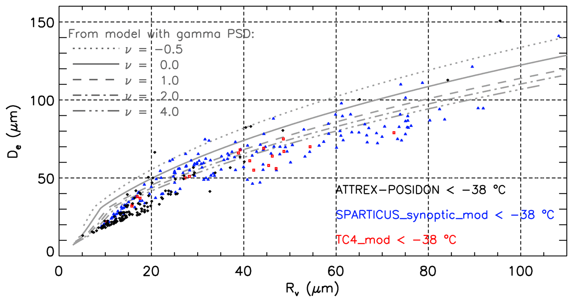
Figure C1 D_e against R_v for the PSDs measured at $T<-\mathrm{38}$ °C during the ATTREX-POSIDON (black), SPARTICUS (navy blue) and TC4 (red) field campaigns where SPARTICUS is based on synoptic cirrus clouds and N(D)₁ was modified for SPARTICUS and TC4. The gray curves are from a model with gamma PSD for 5 values of the PSD dispersion parameter, ν, between −0.5 and 4, illustrating that PSD shape affects the D_e–R_v relationship.