Impact of atmospheric turbulence on the accuracy of point source emission estimates using satellite imagery

Observation-based monitoring of the status of greenhouse gas emissions goals set at the 2015 Paris Climate Summit is critical to provide timely, accurate and precise information on the progress towards these goals. Observations also permit the identification of potential deviations from the adopted policies that could compromise the efforts to reduce the future impact of pollutants on the climate.

Current remote sensing capabilities of atmospheric CO₂ have demonstrated the ability to estimate emissions from the strongest sources of CO₂ based on imagery of individual plumes in conjunction with wind speed estimates. However, a realistic evaluation of the accuracy of the obtained estimates is essential. Here, we examine how the stochastic nature of daytime atmospheric turbulence affects the estimation of CO₂ emissions from a lignite coal power plant in Bełchatów, Poland. For this investigation, we use a high-resolution (400 m × 400 m × 85 levels) atmospheric model set up in a realistic configuration. We demonstrate that persistent structures in the downwind concentration fields of emitted plumes can cause significant uncertainties in the retrieved fluxes, on the order of 10 % of the total source strength, when the commonly used cross-sectional mass-flux (CSF) method is applied with short distances between individual estimates. These form a significant contribution to the overall uncertainty which remains unavoidable in the presence of atmospheric turbulence.

Furthermore, we applied temporally tagged tracers for the decomposition of the plume variability into its constituent parts. These tracers helped us to explain why spatial scales of variability in plume intensity are far larger than the size of turbulent eddies – a finding that challenges previous assumptions.

1 Introduction

The importance of greenhouse gases (GHGs) for the Earth's climate, particularly CO₂, has been established for decades now. Their emissions to the atmosphere remain high and, more importantly, above the optimal pathway that would assure limited climate change, represented by a 1.5 °C mean atmospheric temperature increase by the end of 21th century against a 1850–1900 baseline (IPCC, 2023). Over the last few decades, a range of international policies have been adopted, aiming to minimize the adverse effects of climate change, with the 2015 Paris Agreement (UN, 2015) being the most recent effort coordinated within the United Nations frameworks. Mitigation plans within the agreement are tightly connected with the annual reporting of the emission rates through National Inventory Reports (NIRs), prepared in order to provide accurate and timely information to the international community. Common methodologies used within NIRs are based on bottom-up statistical methods that, in many cases, rely on indirect (proxy) datasets characterized by varying degrees of accuracy (Eggleston et al., 2006). Inconsistencies still exist, especially in underdeveloped countries, which affects our ability to formulate informed and socially acceptable policies to mitigate and adapt to climate change. The provision of transparent and accurate NIRs has a critical impact on building and maintaining societal trust, which is especially important as emission reduction and climate mitigation policies can incur significant societal costs, both monetary and otherwise. Independent, science-based observations of GHG emissions offer a promising approach to enhance the confidence of all stakeholders.

Two issues affect our ability to provide accurate regional budgets of GHGs. First, ground-based networks do not have sufficient density to feed the models that would help to estimate the anthropogenic fluxes at sufficient accuracy where the strongest emissions occur (China, EU, India and USA; see Janssens-Maenhout et al., 2019). Second, in developing countries, where the emissions are smaller but are characterized by larger uncertainties, the ground-based observations are either sparse or missing altogether. Airborne and spaceborne platforms have an important role in filling the observation gap as they can provide information at high spatial resolutions in the regions where only limited (or no) ground-based observations are available. Because of the limitations in terms of range, high unit costs and sparse temporal coverage, the relevance of airborne observations for direct emission estimation at the global or regional scales has historically been largely limited to constraining natural fluxes (Gerbig et al., 2003) or validation of global models (Gałkowski et al., 2021), but, in recent years, robust studies covering larger regions have been conducted, especially concerning emissions from oil and gas industries (e.g. Sherwin et al., 2024). Airborne observations of in situ mole fractions have been successfully used to provide important insights into the subregional and local sources of anthropogenic GHG emissions, employing either pure data-focused analysis (Lowry et al., 2001; Turnbull et al., 2011), mass-balance estimations (Cambaliza et al., 2014; Klausner et al., 2020; Fiehn et al., 2020) or formal inversions of varying complexity (Krings et al., 2018; Lopez-Coto et al., 2020; Kostinek et al., 2021).

Rapid developments in remote sensing instrumentation have opened the avenue for direct estimations of GHG emissions. Although remote sensing instruments installed on airborne platforms have been used successfully for this purpose in the past (Krings et al., 2013; Thorpe et al., 2016; Krautwurst et al., 2021; Wolff et al., 2021), satellite observations offer a distinct advantage due to their global coverage and lower cost per observation. The newest generation of spaceborne sensors has already demonstrated the ability to estimate emissions of pollutants from larger emitting regions and also from single sources – if sufficiently strong. For example, OCO-2 and OCO-3 observations were used to estimate CO₂ emissions from selected large cities and power plants (Nassar et al., 2017; Reuter et al., 2019; Fuentes Andrade et al., 2024), and satellites like GHGSat-D and MethaneAir have shown promise in detecting localized CH₄ plumes with rapid emission estimation (Jervis et al., 2021; Chulakadabba et al., 2023). These successful deployments further motivate the development and use of an operational chain of dedicated satellite missions. Early steps towards such a system were taken through the proposed Earth Explorer mission CarbonSat (Bovensmann et al., 2010). This work was subsequently expanded and resulted in the design and approval of CO2M (Copernicus Anthropogenic CO₂ Monitoring Mission), a constellation of satellites that are to be launched within the current decade (Sierk et al., 2021) and that will form the backbone of the operational system with the CO₂ emission monitoring and verification support (MVS) capacity, as described by Janssens-Maenhout et al. (2020).

A variety of methods have been applied to estimate GHG emissions using either actual remote sensing observations or synthetic data that emulate such observations. A good general description of these methods, their assumptions, and their respective strengths and weaknesses is available in Varon et al. (2018). Of the four methods listed in that study, the Gaussian plume inversion (GPI, Krings et al., 2011; Nassar et al., 2017), the integrated mass enhancement (IME, Frankenberg et al., 2016) and the cross-sectional flux methods (CSF, Krings et al., 2011) have been widely used in practical applications in recent years. Current developments include improvements in plume detection algorithms, also by using auxiliary NO₂ measurements (Kuhlmann et al., 2019, 2021), robust statistical analyses of emission estimates from repeated scenes by a single spaceborne instrument (Nassar et al., 2022; Fuentes Andrade et al., 2024; Santaren et al., 2025) and detailed bottom-up information for comparisons (Nassar et al., 2022; Fuentes Andrade et al., 2024). Across these studies, the reported total emission uncertainty estimated from a single satellite image usually remains between 10 % to 20 % even under the most favourable conditions, i.e. when analysing simple point sources (like power plants) in a cloud-free atmosphere with small gradients in the background fields.

Significant variability exists in the methodology of reporting uncertainty. Uncertainty associated with wind speed estimation has been recognized as one of the most significant (Varon et al., 2018), especially under low wind speeds. No standardized method of uncertainty evaluation has yet emerged, however, resulting in large discrepancies in reported uncertainty estimates. Fuentes Andrade et al. (2024), for example, reported that uncertainty in the wind speed estimation contributes between 24 % and 82 % to the total reported emission uncertainty for nine analysed cases with wind speeds between 3.4 and 9.1 m s⁻¹. In an earlier study based on 10 OCO-3 scenes, Nassar et al. (2022) reported a similar range of uncertainties throughout the sample. However, when only considering the scenes in common with the study of Fuentes Andrade et al. (2024), significantly different total uncertainties were reported. Other error components recognized as significant included the instrument precision (Varon et al., 2018; Kuhlmann et al., 2019), background (Kuhlmann et al., 2019, 2020) and plume rise (Nassar et al., 2022); e.g. Kuhlmann et al. (2020) consider a “method error” that represents the intrinsic uncertainties of the method that arise from simplified assumptions. Large discrepancies between methodologies of error estimation make it difficult to realistically estimate the uncertainty ranges for existing and upcoming satellite missions.

Another major contribution to the reported uncertainty stems from spatial variability due to stochastic turbulence present in the daytime atmosphere (which is when virtually all relevant observations have been collected so far), not explicitly accounted for in any of the methods applied to spaceborne or airborne data. The first analysis of this spatial variability in atmospheric CO₂ was applied to the vertical distribution of CO₂ by Gerbig et al. (2003) and augmented by Lin et al. (2004) to assess representation errors associated with the spatial grid resolution of transport models typically used in inverse modelling. A similar approach to the one used in those studies has been applied in a recent study by Fuentes Andrade et al. (2024) to estimate the uncertainty of emission estimates due to turbulent dispersion (dubbed “dispersion uncertainty”), separating the impact of correlated structures in the CSF method (see Fig. 5 in that study).

Here, a corresponding method is deployed to assess the scales of variability at a somewhat higher spatial resolution, as apparent in partial columns in simulated plumes of CO₂, to assess the impact on the uncertainty of point source emissions and to provide insights into the mechanics influencing emission estimates from the CSF method. We propose that there is a connection between the local wind at the emission point and time and the apparent emissions estimated downwind. That connection is established at the moment of emission and remains in the advected CO₂ signal over distances larger than the eddy scale. Air parcels under low local wind would be loaded with higher mole fractions as the dilution into the atmosphere is lower, while, under higher wind speeds, the dilution into the atmospheric air parcel is larger. We further argue that this variability in mole fractions persists in the downwind advected plumes, causing variability in the apparent emissions reported in the measurements. In order to shed light on these phenomena, we employ high-resolution WRF (Weather Research and Forecast)-GHG simulations over a previously studied point source, enhancing the modelling system with temporally tagged tracers.

The paper is structured as follows: Sect. 2 is dedicated to the description of the experimental setup, study area and model configuration. A detailed description of the temporally tagged tracer concept and application is provided as well. Section 3 presents the results, and Sect. 4 presents a discussion of the results. The conclusions and outlook are presented in Sect. 5.

2 Methods

2.1 Study area

The Bełchatów power plant (BPP) is one of the largest anthropogenic CO₂ point sources globally, relying on lignite coal for power generation. The nominal capacity of the plant was 5102 MW of electrical power in 2021, approximately 13 % of the total capacity of the Republic of Poland (https://pgegiek.pl/Nasze-oddzialy/Elektrownia-Belchatow, last access: 30 August 2024). Under both national and EU legislation, accurate information on GHG emissions and operational status is publicly available, making the BPP an excellent target for developing and testing new instruments and methods. In fact, the BPP has already been used in several studies focusing on developing emission estimation methods (Nassar et al., 2022; Fuentes Andrade et al., 2024) or modelling approaches (Brunner et al., 2023).

The power station is located at 51.267° N, 19.325° E, in the vicinity of Bełchatów in central Poland. Emissions of CO₂ and other compounds are reported through the European Pollutant Release and Transfer Register (E-PRTR). Reported emissions of CO₂ from 2018 to 2022 varied between 30.1 and 38.4 Mt CO₂ yr⁻¹, with a minimum in 2020 (EEA, 2023). The topography of the surrounding area is mostly flat and characterized by minor orographic variability, with notable exceptions being the deep (up to approximately 200 m) open-pit lignite coal mine located directly to the south of the power plant, neighboured by the coal heap containing the residue of the mining operation (up to 175 m high) to the southeast (Fig. 1). The area of the mine pit was approximately 12 km² in 2020.

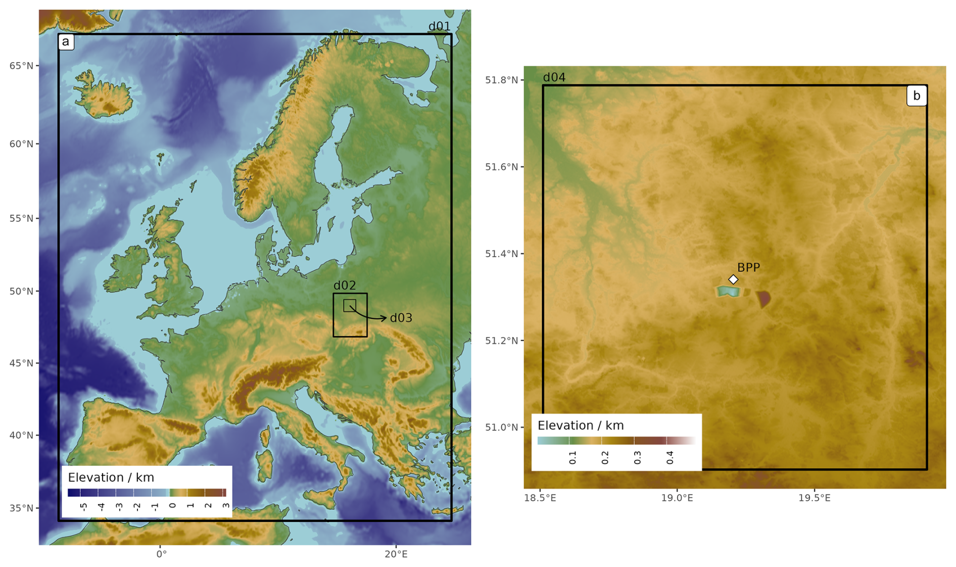
Figure 1 WRF domains for the simulations superimposed onto a topography map. (a) Extent of parent and nested domains. (b) High-resolution domain. BPP denotes Bełchatów power plant, the location of which is marked with a white rhombus.

2.2 WRF-GHG

The numerical experiment presented here was performed using the Weather Research and Forecast Eulerian model WRF (Skamarock et al., 2008) with the Advanced Research WRF (ARW) core enabled. WRF was developed within a large collaborative project led by the National Center for Atmospheric Research (NCAR) and has been augmented over the years by improvements from a number of community users. The model integrates the non-hydrostatic, fully compressible flux form Euler equations on a terrain-following mass-based vertical coordinate and has been successfully applied for meteorological and tracer transport studies at scales ranging from global to local thanks to the ability to dynamically downscale the computations through a nesting algorithm.

For our experiment, we employed WRF v3.9.1.1., with the addition of the GHG module (Beck et al., 2011), implemented within the WRF-Chem (Grell et al., 2005; Ahmadov et al., 2009). Hereafter we refer to this framework as WRF-GHG. The module allows for the emission, transport and mixing of inert CO₂ tracers, as well as online calculation of photosynthetic and respiration fluxes, although that feature was not used in the current study. We applied the system in a limited-area mode, using meteorological boundary conditions from the ECMWF Integrated Forecasting System HRES run, downloaded at 0.125°×0.125° horizontal and L137 vertical resolution (ECMWF, 2022).

The model was run in a one-way nested configuration with three domains of gradually increasing spatial and temporal resolution (Fig. 1). The parent domain spanned continental Europe with a 10 km horizontal grid. The intermediate nested domain covered parts of southern and central Poland at 2 km horizontal resolution, and the final nested domain was run at 400 m horizontal resolution and spanned a rectangular area of 100 km × 100 km, centred around the BPP. To ensure model stability, the domains were run with time steps of 50, 10 and 2 s, respectively. We used the classical mass-based terrain-following η coordinate definition, with the model top set at a constant p=50 hPa, corresponding to approximately 20 km a.m.s.l. As the vertical transport of tracers was one of the key phenomena investigated in our experiment, we have also used a high-resolution vertical level structure in the lower atmosphere, with 85 full-model levels between the surface and the model top. The lowest layer thickness was set to 25 m, with 38 levels below 3 km altitude.

We have used WRF parameterizations suitable for the spatio-temporal scales involved, including the Thompson microphysics scheme, RRTMG schemes for longwave and shortwave radiation, the revised MM5 scheme for surface layer physics, and the Noah Land Surface Model. Grell 3D cumulus parameterization was enabled in the parent domain only. Full-model settings (including all relevant citations) are provided in Table S1 in the Supplement. As the nested domains are run at horizontal resolutions in the so-called “grey zone” (i.e. grids with horizontal spacing between 0.2 and 6 km; see Honnert et al., 2020), we have applied the Shin–Hong PBL (planetary boundary layer) scheme (Shin and Hong, 2015) for all simulated domains. This parameterization introduces scale dependency for vertical transport in the convective PBL and follows the YSU scheme in the free atmosphere. We have used the default MODIS land use category maps (at 30^′′) and elevation maps (at 1^′ resolution for the parent domain and 30^′′ for nested domains). Grid nudging was applied in the parent domain to maintain wind, temperature and moisture fields consistent with the driving meteorological data at a continental scale. We did not apply any nudging to the intermediate and high-resolution domains to allow the WRF internal parameterizations to drive the tracer transport at smaller scales. The strength of the nudging coefficient for water vapour was reduced to $\mathrm{4.5}\times {\mathrm{10}}^{-\mathrm{5}}$ m s⁻¹ following Spero et al. (2018).

Prior to data analysis, simulated CO₂ fields were interpolated from WRF's Lambert Conformal Conic projection to a time-varying Cartesian coordinate system centred at the BPP and oriented towards the direction of the effective wind (u_eff), calculated every minute as an average of local wind speeds sampled between 200–600 m a.g.l. over a square area (20 km × 20 km) surrounding the BPP. The height range was selected as the applied emissions are distributed mostly in this range (see the following section).

The vertical structure of the original WRF grid was preserved exactly, while the horizontal resolution was increased 2-fold in order to better preserve the spatial features of the modelled plume (200 m × 200 m), using bilinear interpolation. The output grid formed a perpendicular area ranging from −5 to +40 km in the X (along-wind) direction and −25 to 25 km in the Y direction in order to capture the full width of the plume throughout the period relevant for the analysis.

2.3 Emissions and tagged tracers

Three individual stacks were responsible for CO₂ emissions at the BPP in 2020. Nassar et al. (2022, Table 4) used publicly available data and found that only blocks B2–B12 of the power plant were operational on 10 April 2020, our date of interest. These blocks emit CO₂ through two tall (300 m high) stacks located 330 m apart. In our model we combined both into a single point source as our horizontal grid size is 400 m. We applied emissions of CO₂ at the constant rate equal to the average annual emissions officially reported by the BPP for the year 2018, i.e. 38.4 Mt CO₂ yr⁻¹ (EEA, 2023). Instead of a dedicated plume rise mechanism, we applied an invariable vertical profile in emissions, with tracer mass distributed along a Gaussian curve centred at $H_{\mathrm{eff}}=\mathrm{4}/\mathrm{3}H$, with a standard deviation of ${\mathit{\sigma }}_{\mathrm{H}}=\mathrm{1}/\mathrm{3}H$, where H is the emitting stack height of 300 m. Examples of emission profiles and resulting model mole fractions are given in Fig. S1 in the Supplement.

The emissions from the stack are subsequently advected in the model throughout the full simulation period. We used this tracer primarily to monitor the spatial extent over which the tracers represent the whole plum and to calculate the dependence of emission estimate statistics over variable distances.

We also used 60 additional tracers tagged by the time of release (temporally tagged tracers) in order to study the effects of atmospheric turbulence on source estimation inference. Each tracer corresponds to a short segment of the emitted plume, together encompassing the full emission signal emitted from the stack over a 3 h time period (see the next section). Segments of 3 min were chosen as a compromise between the desire for maximum detail and computational constraints. This time was sufficient to represent wind variability at the emission point. The numerical tests have shown only a 1.5 % loss of variance when using 3 min averaged output as compared to instantaneous 1 min output.

The resulting CO₂ signals are conceptually similar to the “particles” or “air parcels” used in Lagrangian models. We refer to these emitted plume segments as “puffs”. The distribution of CO₂ mole fractions for a selection of puffs is presented in Fig. S2, and an example XCO₂ from a single puff is plotted in Fig. 4 (see Sect. 3) against the full plume extent.

Using these short puffs allows us to evaluate the impact of large eddies interacting with the tracer at the point of emission, as well as during their advection to further downstream areas. For this we specifically calculate plume centroids to follow the motion of each puff (details in Sect. 2.8.1), as well as the wind speed during the time of the tracer release, which directly impacts the initial dilution of the tracer when emitted into the atmosphere (detailed in Sect. 2.8.2).

2.4 Simulated case

For our study, we ran the simulation for a period between 18:00 UTC on 9 April 2020 and 21:00 UTC on 10 April 2020. These dates were selected as good candidates as OCO-3 observations from that day displayed characteristic variability of apparent emissions that we investigate in this study. In the model, we emitted 60 puffs between 09:00 and 12:00 UTC (11:00–14:00 LT) in successive 3 min periods. The numerical analysis of the output was performed when the final tracer was emitted completely, i.e. at 12:00 UTC. By that point, the oldest tagged tracers had already been advected through the modelling domain for 3 h. We stored the 1 min output for the high-resolution domain from 09:00 until 21:00 UTC for maximum temporal coverage over the analysed day.

2.5 Column-averaged mole fractions

The column-averaged dry-air mole fraction, commonly used in remote sensing measurements, is a scalar quantity that integrates trace gas abundances across the whole atmospheric column. It offers advantages over reporting in mass units as it reduces the influence of surface pressure and topography on the retrieved signals. For every output time, WRF-GHG provides 3D fields of dry-air mole fraction enhancements (designated as ΔC for the full plume tracer), from which we calculate column-averaged dry-air mole fraction using the following formula:

$$\begin{array}{}\text{(1)}& \mathrm{\Delta }X{C}_{ij}=\sum _k\mathrm{\Delta }{C}_{ijk}{\mathit{\omega }}_{ijk}.\end{array}$$

Here, ΔXC_ij is the enhancement of the column-averaged dry-air mole fraction of CO₂ at coordinate (x_i, y_j) of the Eulerian grid. ΔC_ijk is the dry-air mole fraction of CO₂ at model grid coordinates (x_i, y_j, z_k), given in mol mol⁻¹, and ω_ijk denotes the weights applied to each value, calculated as

$$\begin{array}{}\text{(2)}& {\mathit{\omega }}_{ijk}={\displaystyle \frac{{\left[n_{\mathrm{d}}\right]}_{ijk}}{\sum _k{\left[n_{\mathrm{d}}\right]}_{ijk}}}={\displaystyle \frac{\mathrm{1}}{N_{\mathrm{d}}}}{\left[n_{\mathrm{d}}\right]}_{ijk}.\end{array}$$

Here, [n_d]_ijk is the number of moles of dry air in the grid cell at x_i, y_j, z_k, and N_d is the total number of moles of dry air throughout the air column. Because our model top was set at 50 hPa, we applied a correction to account for the missing atmospheric mass when calculating the weights. The formulas above are independent of axis orientation, but the values discussed are in the wind-rotated coordinate system, with the x axis being oriented along the wind direction.

2.6 Cross-sectional flux method of estimating apparent emissions

By assuming that the mass of the tracer is conserved (true in the case of long-lived greenhouse gases advected over short distances), emission rates at the source can be inferred by integrating the tracer mass elements passing through a plane perpendicular (i.e. along the y axis) to the wind direction at a certain distance x downstream from the source. This can be described mathematically as follows:

$$\begin{array}{}\text{(3)}& \mathrm{\Phi }\left(x\right)=u_{\mathrm{eff}}\underset{-\mathrm{\infty }}{\overset{\mathrm{\infty }}{\int }}\mathrm{\Delta }\mathrm{\Omega }(x,y)\mathrm{d}y.\end{array}$$

Here, x and y denote coordinates (in m) in the rotated Cartesian grid, with the x axis being oriented along the wind direction. Φ(x) denotes the estimated emission (further referred to as the “apparent emission”) at cross-sections computed at x (in kg s⁻¹). ΔΩ(x,y) is the column-integrated enhancement of CO₂ (in kg m⁻²), and u_eff is the effective wind speed in the direction along the x axis (given in m s⁻¹). It should be noted that the equation is true when turbulent flux along the x axis is small compared to the advective flux characterized by u_eff. An excellent overview of the turbulent and advective flux terms is available in Conley et al. (2017), who show that, when winds are close to and below this threshold, upwind-directed fluxes may cause overestimation of the scalar source strength for near-surface point sources. Varon et al. (2018) have argued that, for a typical turbulent day, this condition is met when wind speeds are 2 m s⁻¹ or higher and used this value as a lower limit of the applicability of the CSF method. We follow the approach of previously published measurement-driven studies that included the analysed case (Nassar et al., 2022; Fuentes Andrade et al., 2024) and assume that the turbulent flux component can be neglected in the downwind areas.

It can be shown that, for the WRF Eulerian grid, ΔΩ(x,y) can be discretized as follows:

$$\begin{array}{}\text{(4)}& \mathrm{\Delta }{\mathrm{\Omega }}_{ij}={\displaystyle \frac{\mathit{\mu }{N}_{\mathrm{d}}}{A}}\mathrm{\Delta }X{C}_{ij}={\displaystyle \frac{\mathit{\mu }}{A}}\sum _k\mathrm{\Delta }{C}_{ijk}{\left[n_{\mathrm{d}}\right]}_{ijk},\end{array}$$

where μ is the molar mass of CO₂ (0.044 kg mol⁻¹), A is the horizontal model cell area in m², and other symbols are as before.

Applying the above to Eq. (3) in its discrete form yields the apparent emission at a given distance x_i as follows:

$$\begin{array}{}\text{(5)}& \mathrm{\Phi }\left(x_i\right)={\displaystyle \frac{\mathit{\mu }{u}_{\mathrm{eff}}}{\mathrm{\Delta }x}}\sum _{j,k}\mathrm{\Delta }{C}_{ijk}{\left[n_{\mathrm{d}}\right]}_{ijk},\end{array}$$

where Δx is the dimension of the model cell along the x axis (in metres). By calculating the sum over a wide range of cross-wind distances (y axis, index j), we made certain that the full plume extent and mass are reproduced in our interpolated fields. Similarly, we also ensured that the plume mass is fully contained in the vertical direction (index k) over the analysis area.

We calculate the effective wind speed u_eff from horizontal wind fields averaged over altitudes surrounding the peak in the emission vertical profile. This approach is a hybrid of those used in the recent studies of Kuhlmann et al. (2021) and Nassar et al. (2022). In the first study, the mean wind speed was calculated from the model output winds, weighted by relative emission strength. The emission profile, however, was based on statistically averaged profiles and did not take into account actual stack heights. In the second study, Nassar et al. (2022) used a Gaussian plume model to simulate the plumes from the BPP, with the plume centreline set at 250 m above the stack height to represent the additional plume rise (H_eff), following Brunner et al. (2019). Subsequently, they used winds from reanalysis datasets extracted at the same height over the emission point to calculate u_eff.

Here, we calculate u_eff as an average of wind speed values at altitudes between H_eff±2σ_H (200–600 m). As we aim to mimic processing as performed in studies using actual satellite imagery, we assume a constant u_eff throughout the area of interest despite having access to complete modelled wind fields. We also spatially average the wind speeds over a square area of ±20 km around the emission point, which mimics the effect of using a coarse-resolution reanalysis wind dataset like ERA5 (as in Nassar et al., 2022) that does not represent variabilities on smaller scales.

In Sect. 3.3, when analysing the behaviour of the apparent emissions in relation to the location of the puffs, we make use of the normalized apparent emission anomaly λ_Φ(x), defined as

$$\begin{array}{}\text{(6)}& {\mathit{\lambda }}_{\mathrm{\Phi }}\left(x\right)={\displaystyle \frac{\mathrm{\Phi }\left(x\right)}{\stackrel{\mathrm{‾}}{\mathrm{\Phi }}}}-\mathrm{1},\end{array}$$

where $\stackrel{\mathrm{‾}}{\mathrm{\Phi }}$ is the average of Φ(x) calculated over the selected x range.

2.7 Effective number of observations and uncertainty of emission

To estimate the mean uncertainty of the apparent flux, we calculate the mean value of Φ from individual cross-sectional flux estimates. Due to the existence of autocorrelation in the CO₂ enhancement on short spatio-temporal scales, the uncertainty of the mean apparent emission $u\left(\stackrel{\mathrm{‾}}{\mathrm{\Phi }}\right)$ is therefore also spatially correlated and follows the standard formula for type-A uncertainty (u_a) as defined in Eq. (3) of Zięba (2010), who, in turn, follows JCGM (2008). With correlation present, the basic formula can be modified by a factor dependent on the effective number of observations n_eff:

$$\begin{array}{}\text{(7)}& u_{\mathrm{a}}\left(\stackrel{\mathrm{‾}}{\mathrm{\Phi }}\right)=u\left(\stackrel{\mathrm{‾}}{\mathrm{\Phi }}\right)\sqrt{{\displaystyle \frac{n-\mathrm{1}}{n_{\mathrm{eff}}-\mathrm{1}}}},\end{array}$$

where the index “a” denotes that the uncertainty is calculated for an autocorrelated sample of n observations. The number of effective observations can be calculated using the autocorrelation function (ACF) following the formula from Zięba (2010):

$$\begin{array}{}\text{(8)}& n_{\mathrm{eff}}={\displaystyle \frac{n}{\mathrm{1}+\mathrm{2}\sum _{\mathit{\kappa }=\mathrm{1}}^{n-\mathrm{1}}\frac{n-\mathit{\kappa }}{n}{\mathrm{ACF}}_{\mathit{\kappa }}}},\end{array}$$

where κ is the lag index of the discrete ACF function.

A similar approach to calculating uncertainty for correlated CO₂ data was applied by Gerbig et al. (2003) for airborne vertical profile data and, more recently, by Fuentes Andrade et al. (2024) to estimate the dispersion error component in remote-sensing-based flux estimates.

2.8 Decomposition of variability into contributions

To further study the plume dispersion dynamics, we calculate and use two additional auxiliary variables: the location of plume centroids along the x axis and the wind speed at the time and location of emission. Their respective definitions and purposes are given below.

2.8.1 Plume centroids

We define a plume centroid as the first moment of the distribution of the tracer's mole fraction, thus approximating each tracer's centre of mass. The location of the pth tracer centroid along the x axis is calculated as follows:

$$\begin{array}{}\text{(9)}& \stackrel{\mathrm{‾}}{x_{\mathrm{p}}}={\displaystyle \frac{\sum _{ijk}\mathrm{\Delta }{C}_{ijk}^{\mathrm{p}}{x}_i}{\sum _{ijk}\mathrm{\Delta }{C}_{ijk}^{\mathrm{p}}}}.\end{array}$$

Here, $\mathrm{\Delta }{C}_{ijk}^{\mathrm{p}}$ denotes the CO₂ dry-air mole fraction enhancement of a single tagged tracer at coordinates x_i, y_j, z_k, as before. The location of the tracer centroids along the y axis, $\stackrel{\mathrm{‾}}{y_{\mathrm{p}}}$, is calculated analogously.

To investigate the relationship between the number of plume centroids at a given distance x_i and apparent emissions Φ(x_i), related to the meandering of the plume, we use the puff centroid density r(x_i), calculated for each x_i as the sum of plume centroids falling within x values in the range $\left[\frac{\mathrm{1}}{\mathrm{2}}\left(x_{i-\mathrm{1}}+x_i\right),\frac{\mathrm{1}}{\mathrm{2}}\left(x_i+x_{i+\mathrm{1}}\right)\right]$. Due to the low number of centroids imposed by the computational constraints, we cannot estimate r directly at the full resolution of our interpolated grid. Instead, we follow a two-step procedure: first we bin centroids at a reduced resolution of 2 km, and then we use a cubic spline interpolation to obtain the centroid density at a full 200 m resolution. r(x_i) and its spatial average $\stackrel{\mathrm{‾}}{r}$ are then used to calculate the normalized anomaly of the centroid density λ_c, analogously to Eq. (6).

2.8.2 Wind speed at emission point and time

The second auxiliary variable is calculated to study how the local, highly variable wind speed at the emission location and time affects the estimates of Φ.

In order to investigate the effect of turbulent winds on the initial dilution mentioned in the Introduction and to assess the extent of the resulting spatial patterns and their impact on the apparent emissions estimated downwind, we calculate wind speed at the emission location: WS_emi(x_i). WS is used to avoid confusion with u_eff. Because the signal in the plume is efficiently mixed, the local wind conditions at the emission point can only be monitored using puffs. Thus, each puff is allocated a mean wind speed at the stack during its time of emission (${\stackrel{\mathrm{‾}}{{\mathrm{WS}}_{\mathrm{emi}}}}^{\mathrm{p}}$), and as the puffs are advected along the plume, the WS_emi(x_i) can be calculated for any given plume element by averaging across its constituent puffs, using their respective mole fractions as weights.

More precisely, for each puff, ${\stackrel{\mathrm{‾}}{{\mathrm{WS}}_{\mathrm{emi}}}}^{\mathrm{p}}$ is calculated as the average of the u wind component (i.e. parallel to the x axis) at the emission point during the 3 min emission time of each tracer over the vertical extent surrounding the stack height:

$$\begin{array}{}\text{(10)}& {\stackrel{\mathrm{‾}}{{\mathrm{WS}}_{\mathrm{emi}}}}^{\mathrm{p}}=\sum _k{\displaystyle \frac{\stackrel{\mathrm{‾}}{u_{\mathrm{p}}}\left(z_k\right)}{n_z}}.\end{array}$$

Here, $\stackrel{\mathrm{‾}}{u_{\mathrm{p}}}\left(z_k\right)$ denotes 3 min averaged values of the parallel wind component (in the x direction) at the stack horizontal coordinates, extracted at altitude z for tracer p. We calculate the average over the vertical range over which the maximum emissions occur, i.e. between 200 and 600 m above ground, and n_z denotes the number of model levels whose centres fall within that range.

In order to link individual puff values with the apparent emission downwind from the emission point, we use a two-step algorithm. First, for each spatial point in our model, we calculate the mean value of $\stackrel{\mathrm{‾}}{{\mathrm{WS}}_{\mathrm{emi}}}$ for that point, weighted by the column-averaged dry-air mole fractions of each puff:

$$\begin{array}{}\text{(11)}& \stackrel{\mathrm{‾}}{{\mathrm{WS}}_{\mathrm{emi}}}\left(x_i,y_j\right)=\sum _{\mathrm{p}}{\stackrel{\mathrm{‾}}{{\mathrm{WS}}_{\mathrm{emi}}}}^{\mathrm{p}}{\mathit{\omega }}_{ij}^{\mathrm{p}},\end{array}$$

where

$${\mathit{\omega }}_{ij}^{\mathrm{p}}={\displaystyle \frac{\mathrm{\Delta }X{C}_{ij}^{\mathrm{p}}}{{\sum }_{\mathrm{p}}\mathrm{\Delta }X{C}_{ij}^{\mathrm{p}}}}.$$

In the second and final step, we calculate the cross-section average WS_emi(x_i) (overbar omitted) by weighting by the XCO₂ column-averaged mole fractions:

$$\begin{array}{}\text{(12)}& {\mathrm{WS}}_{\mathrm{emi}}\left(x_i\right)=\sum _j\stackrel{\mathrm{‾}}{{\mathrm{WS}}_{\mathrm{emi}}}\left(x_i,y_j\right){\mathit{\psi }}_{ij},\end{array}$$

with the weights ψ_ij being calculated as

$${\mathit{\psi }}_{ij}={\displaystyle \frac{\mathrm{\Delta }X{C}_{ij}}{\sum _j\mathrm{\Delta }X{C}_{ij}}}.$$

In the subsequent analysis, we correlate WS_emi(x_i) with Φ(x) in order to assess the imprint of the initial wind speed on the apparent emissions estimated downwind of the source. To avoid potential numerical noise caused by calculating ratios for low values, we limited the analysis to those model grid points for which the total simulated CO₂ enhancements were higher than 0.01µmol mol⁻¹.

3 Results

3.1 Wind speed and direction

The simulated meteorological conditions show a nocturnal stable atmosphere evolving into a turbulent PBL over the course of the morning (05:00–11:00 UTC). By 11:00 UTC, the turbulence in the lower atmosphere has already been established, with a gentle westerly wind of almost 3 m s⁻¹ at the emission point. The local horizontal wind components show increasingly strong variations against the mean effective wind from 09:00 UTC onwards (Fig. 2). By 12:00 UTC the turbulent conditions were fully developed in the local atmosphere, with the wind speed variations growing from 1.5 m s⁻¹ peak to peak at 10:00 UTC to approximately 3.0 m s⁻¹ at 12:00 UTC, with a mean horizontal area-averaged wind of 2.856±0.007 m s⁻¹. The simulated local wind direction deviated northwards from the mean by approximately 15° between 09:00 and 10:00 UTC. Afterwards, the oscillations of the wind direction became random, varying between 300 and 340°, with a frequency similar to the variations in wind speed.

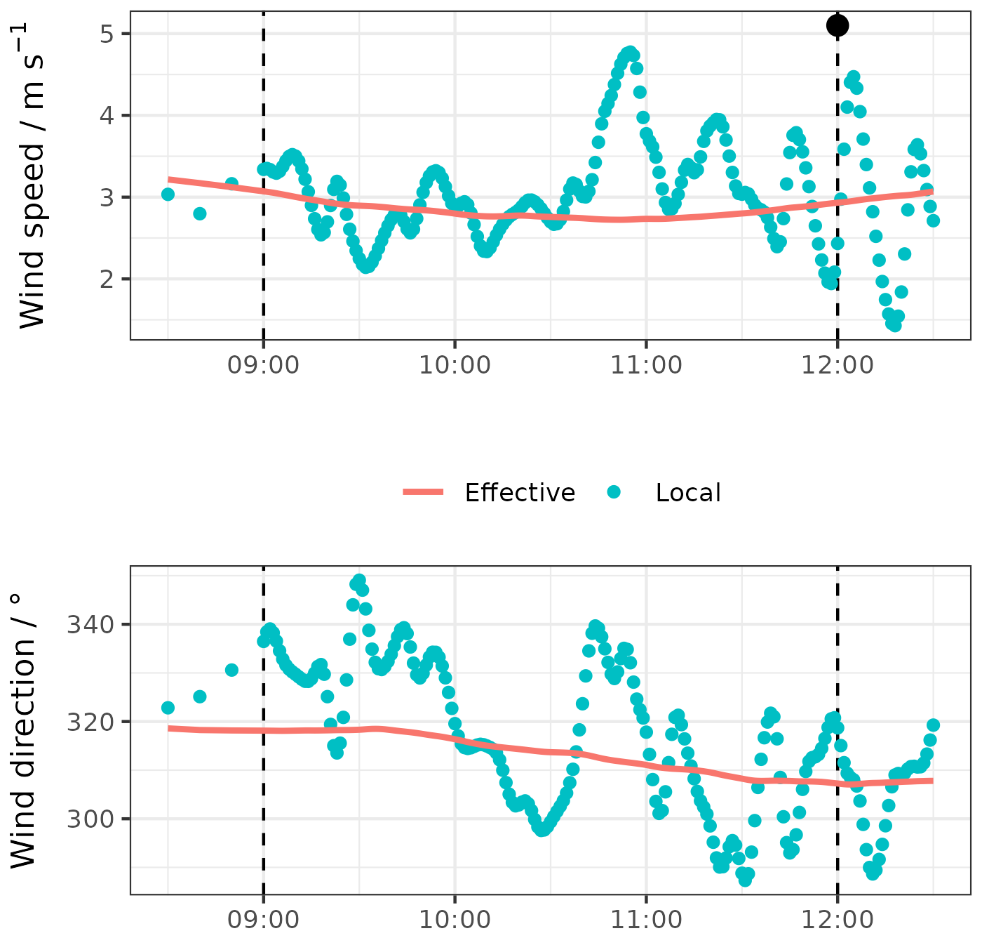
Figure 2 Simulated horizontal wind speed and direction at the emission point, averaged over the vertical extent of the majority of emissions (200–600 m; see Sect. 2.6). Values at the emission point (local) are shown in blue, and effective wind, averaged over a larger area, is shown in red. See the Methods section for details. Dashed lines denote the start and end of the puff tracer emissions. For these, the model output was stored every 1 min. The black dot at the top of the second dash denotes the moment at which the simulated scene was collected.

3.2 Simulated plume structure

In our analysis, we focused on the state of the atmosphere at 12:00 UTC (14:00 CEST), 1 h and 14 min after the local solar noon (10:44 UTC on 10 April 2020), when the PBL was already well developed and the CO₂ plume emitted from the BPP had been advected and mixed for several hours. This is consistent with typical observation times of passive remote sensing instruments operated on platforms in sun-synchronous orbits as overpass times near local solar noon provide a high signal-to-noise ratio.

Figure 3 presents a set of cross-sections of the simulated CO₂ plume at 12:00 UTC. As shown, the model simulates a turbulent plume to a distance of 40 km from the emission source, with significant dispersion in both the horizontal (x, y) and vertical (z) directions. High mole fractions close to the emission source, reaching around 1000 µmol mol⁻¹, are quickly dispersed by advection and turbulence, already dropping to below 60 µmol mol⁻¹ 5 km downwind from the source, and these are further reduced as dispersion spreads the mass of the tracer perpendicularly to the main wind direction. Notably, the model predicts very efficient vertical mixing of the emitted tracer from the surface to the top of the PBL (located at 1.6 km at 12:00 UTC). When averaging the plume along the x axis across the whole analysis area, the tracer mass is distributed almost uniformly up to the PBL top, distributed primarily around y=0 across the plume, with a skew towards positive y values (Fig. 3, lower right).

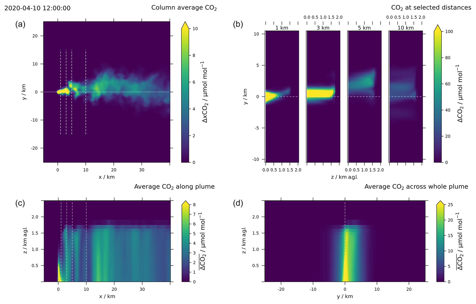
Figure 3 Simulated plume structure at 12:00 UTC on 10 April 2020. (a) Column-averaged CO₂ emitted from the BPP. Cross-sections presented on the right are marked with dashed lines. (b) CO₂ enhancements simulated at cross-sections located 1, 3, 5 and 10 km downwind from the emission source. (c) Cross-section of mole fractions averaged across the X–Z plane. (d) Average CO₂ mole fraction enhancement in the Y–Z plane calculated across all distances (−5 to 40 km).

We compared the emitted total CO₂ tracer with the sum of the 60 puffs to make certain that no notable differences in the overall plume structure are caused by the numerical effects of the WRF advection schemes applied. These occur due to different gradients present in the tagged and total tracer fields. At 12:00 UTC, which marks the end of the period of puff emissions, the plume is fully represented at distances from the emission point of 0 km down to approximately 22 km. Local discrepancies between the sum of tagged tracers and the classical full tracer are caused by the advection scheme. Point-wise differences in mole fractions of the two plume realizations can reach as high as 1000 µmol mol⁻¹ in the immediate vicinity of the emission point, while they become much smaller further downwind from the plume as the mixing effectively reduces spatial gradients in the tracer field (Fig. S3). To avoid any potential disturbances due to these numeric effects and also to avoid representation errors due to insufficient spatial resolution in the near field, we have excluded data from the first 2 km downwind of the BPP from the analysis. We have found that the model mass conservation scheme works well, with the total mass of both plume versions agreeing within 0.035 % at distances between 2 to 22 km; thus, we treat both realizations of the plume as identical. See Sect. S4 in the Supplement for details.

3.3 Inferring point source rate using cross-sectional estimates

Undulations are visible in the column-averaged tracer (Fig. 4), which, in turn, leads to significant variability in the apparent emission rate calculated across the downwind distances (Fig. 5). The predicted Φ values vary between 22.5 and 70.0 Mt yr⁻¹, respectively, 59 % and 182 % of the actual emission rate of 38.4 Mt yr⁻¹. While the oldest puffs have been advected to over 30 km downwind from the source, the range over which they are equal to the full-signal tracer is only identical up to approximately x=22 km. Beyond that distance, a steadily increasing fraction of the crosswind-aggregated signal comes from CO₂ emitted before 09:00 UTC. Therefore, we focus on values at downwind distances between 2 km < x < 22 km for the subsequent quantitative analysis.

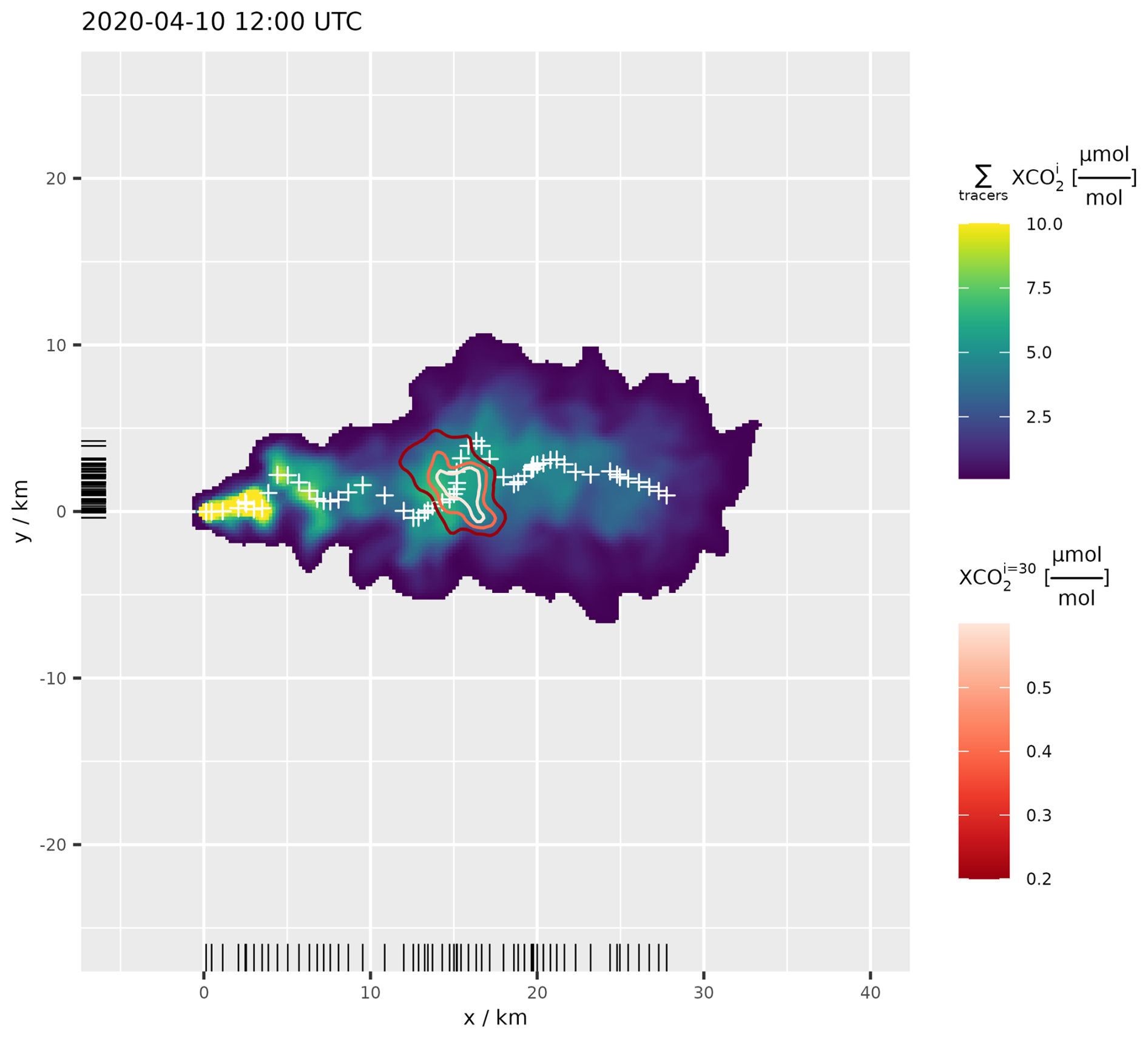
Figure 4 Simulated plume structure at 12:00 UTC on 10 April 2020. XCO₂ of the full CO₂ plume (blue-yellow scale) fragment, with the distribution of a single puff (co2_bpp_30) shown in red-white contours (scaled by mole fraction). Values lower than 0.1 ppm were omitted for clarity. Centroid positions [$\stackrel{\mathrm{‾}}{x_{\mathrm{p}}}$, $\stackrel{\mathrm{‾}}{y_{\mathrm{p}}}$] of puffs are marked with white crosses, and rug marks on the x and y axes show their respective distributions.

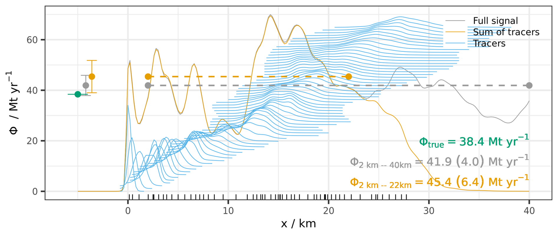
Figure 5 Apparent emissions Φ(x) downwind from the emission point calculated using the full simulated plume (grey) and the sum of the tagged tracers (orange). Contributions from individual tagged tracers are marked in blue (offset by a constant value for display purposes). Horizontal dashed lines mark the distance ranges over which the average emissions were estimated. Points to the left of the emission point compare true emissions in the model against computed averages with their uncertainty.

Using the simulated fields, we estimated the mean emission from the source as an average of Φ(x) values at individual cross-sections, yielding 45.4 Mt yr⁻¹. We then calculated the autocorrelation function of the apparent emission (Fig. 6) to estimate the n_eff. We assumed that the ACF overshoot for values above 4 km is primarily due to the moderate sample size and can be ignored. Therefore, for the n_eff calculation, we set the terms beyond the first zero-crossing (at approximately x=4 km) to zero, yielding n_eff equal to 5.56, corresponding to an independent measurement occurring every 3.6 km. The calculated 1σ uncertainty of the mean emission is equal to 6.4 Mt yr⁻¹ (14.2 % of the mean); thus, the true emission value of 38.4 Mt yr⁻¹ falls outside of the calculated 1σ range by 0.6 Mt yr⁻¹.

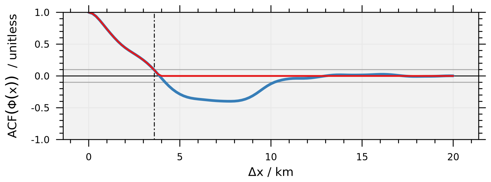
Figure 6 Blue: ACF of Φ(x) (blue), calculated for 2  km ≤ x ≤ 22 km. Red: simplified ACF used for calculating n_eff. The vertical dashed line denotes the distance between independent observations (d_indep) corresponding with the calculated n_eff.

Table 1 Estimated emission statistics.

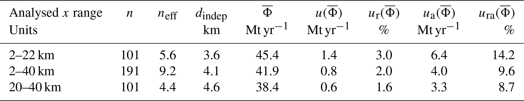
Note that n denotes the number of observations; n_eff denotes the effective number of observations; d_indep denotes the distance between independent observations; $\stackrel{\mathrm{‾}}{\mathrm{\Phi }}$ denotes the average apparent emission; $u\left(\stackrel{\mathrm{‾}}{\mathrm{\Phi }}\right)$ denotes the absolute uncertainty of the mean apparent emission without taking into account autocorrelation; $u_{\mathrm{r}}\left(\stackrel{\mathrm{‾}}{\mathrm{\Phi }}\right)$ is the relative uncertainty of $\stackrel{\mathrm{‾}}{\mathrm{\Phi }}$; $u_{\mathrm{a}}\left(\stackrel{\mathrm{‾}}{\mathrm{\Phi }}\right)$ denotes the absolute uncertainty of the mean apparent emission, modified to take autocorrelation into account; and $u_{\mathrm{ra}}\left(\stackrel{\mathrm{‾}}{\mathrm{\Phi }}\right)$, as before, is relative.

Using the full-tracer signal rather than the sum of tagged tracers allowed us to also evaluate the effect of calculating the mean emission rate from different plume subsets: a long one, with cross-sections taken between 2 and 40 km, and a short subset that was calculated between 20 and 40 km. This allowed us to test whether increasing the distance over which apparent emissions are estimated improves the precision of the emission estimates. Indeed, when the longer segment of the plume is analysed, the mean estimated emission was yielded to be 41.9±4.0 Mt yr⁻¹ (relative uncertainty of 9.6 %). An even more accurate emission estimate is obtained when using cross-sections from 20 to 40 km plume fragments, with $\stackrel{\mathrm{‾}}{\mathrm{\Phi }}=\mathrm{38.4}\pm \mathrm{3.3}$ Mt yr⁻¹. The results are summarized in Table 1.

When analysing the spatial distribution of plume centroids (white crosses in Fig. 4), a meandering pattern is visible, caused by high-frequency variability in the wind fields downwind from the emission source. This meandering results in an uneven distribution of the centroids along both the x and y axes (rug marks, Fig. 4). In order to quantify the effect on apparent emission estimates at given downstream locations, the normalized anomaly of the puff density λ_c has been calculated as described in Sect. 2.8 and is shown in Fig. 7a. The centroid density anomaly is positively correlated with the corresponding apparent emission estimates (R²=0.54, Fig. 7b).

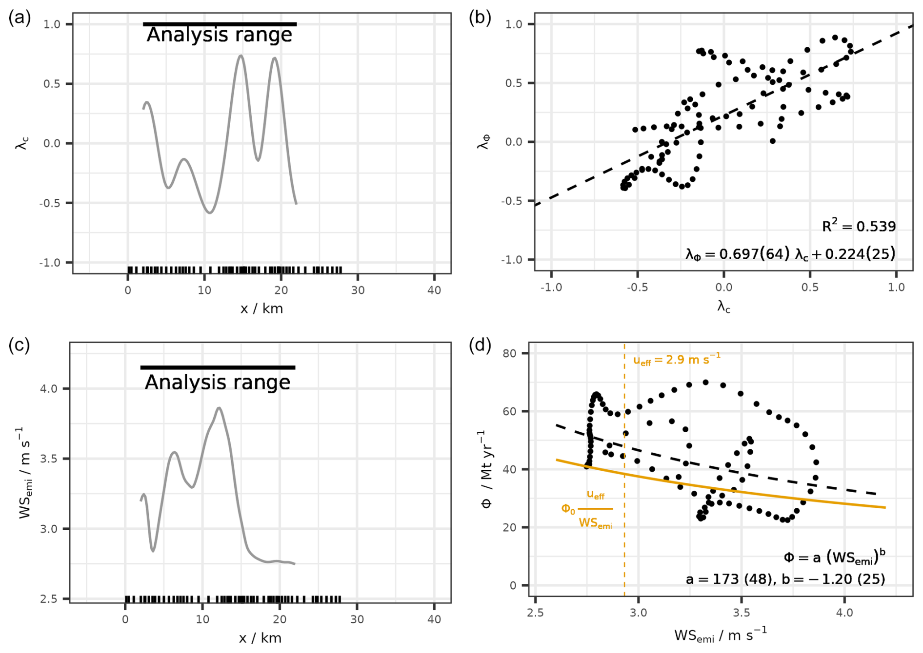
Figure 7 (a) Normalized anomaly of puff centroids (λ_c) per distance. (b) Correlation of normalized anomaly of apparent emission (λ_Φ) with λ_c. (c) Weighted average of parallel wind component at emission time (WS_emi) vs. distance. (d) Correlation between WS_emi and Φ(x), together with the theoretical curve and fitted hyperbolic curve.

We have also analysed the correlation between the apparent estimated emissions and WS_emi (shown separately as a function of x in Fig. 7c). Φ(x) is observed to decrease with WS_emi at an average rate of 18.1 Mt yr⁻¹ per every 1 m s⁻¹ of wind (Fig. 7d); however, the correlation of a linear fit is weak (R²=0.20).

In order to understand how the dilution of CO₂ at the emission point due to local wind variability affects the apparent emissions, it is worthwhile to consider a simplified 1D theoretical model of the relationship between the local horizontal wind at the emission point and the apparent emissions. Given constant emissions (Φ₀) and effective wind speed (u_eff), the deduced emissions downwind (which are proportional to the downwind concentration enhancement, as per Eq. 5) should be inversely proportional to the instantaneous (turbulent) wind speed at the time of the emissions (WS_emi), i.e.

$$\begin{array}{}\text{(13)}& \mathrm{\Phi }\propto {\mathrm{\Phi }}_{\mathrm{0}}{\displaystyle \frac{u_{\mathrm{eff}}}{{\mathrm{WS}}_{\mathrm{emi}}}}.\end{array}$$

We have added the theoretical curve following Eq. (13), assuming that the proportionality factor equals exactly 1, as seen with the yellow line in Fig. 7d, using u_eff=2.9 m s⁻¹ (value at 12:00 UTC). We have also added a non-linear least-squares regression to fit a power curve (Φ=a(WS_emi)^b) to the data, yielding an exponent b equal to $-\mathrm{1.20}\pm \mathrm{0.25}$. As expected, the empirical formula fits the data better. The difference between the theoretical curve is expected as the assumptions for such a simple model are not fulfilled in a realistic three-dimensional case.

4 Discussion

Our model setup captured the characteristics of the point source plume structure well. The estimated cross-section emissions show typical features of the pollutant plume in terms of horizontal and vertical dispersion. Virtually all of the CO₂ plume is contained within 10 km from the main wind axis, and most of the mass is concentrated within 5 km, similarly to the extent observed by OCO-3 and as reported earlier (Figs. 3 and 4 here; Nassar et al., 2017; Fuentes Andrade et al., 2024). It is likely that vertical mixing is overestimated in the direct vicinity of the emission point, which is at least partially caused by the use of a Gaussian emission profile rather than having the plume rise mechanism implemented directly in the model. This potential inaccuracy becomes less relevant with distance as vertical mixing efficiently distributes the tracer throughout the PBL. The variability in the apparent emissions predicted by the model is similar to that based on remote sensing observations from the same day, with a modelled 1σ_Φ of 4.0 Mt yr⁻¹, calculated here for distances between 2 and 40 km vs. the 3.4 Mt yr⁻¹ dispersion uncertainty (of 6.4 Mt yr⁻¹ total) estimated by Fuentes Andrade et al. (2024).

The number of independent observations appears to be in good agreement as well, with our modelling framework predicting an independent Φ estimate every 3.6 km compared to one every 2.9 km, as estimated by Fuentes Andrade et al. (2024) using a slightly different approach. Based on the above, we conclude that the overall plume structure is realistic, which gives us confidence that the tagged tracers propagated via the model also realistically depict the distribution of the tracer mass, confirming the high capability of WRF-GHG, previously reported by Brunner et al. (2023). This is an important conclusion as this assumption is virtually impossible to test directly in the field.

In order to estimate the influence of the turbulence on the precision of emission estimation, we have calculated the mean apparent flux for two plume segments, namely for the full available plume distance, using the full tracer (2–40 km) and a shorter one (2–22 km), corresponding to the section of the plume fully resolved by the tagged tracers. In both instances, we have estimated the mean emission uncertainty following the algorithm provided in Sect. 2.7. When the correlation of observations is taken into account, the uncertainties of the emission estimate become significantly higher, in our case increasing by a factor of 4 (Table 1). The extra uncertainty stems from correlation in the Φ(x_i) that occurs due to turbulent dispersion, and it reduces the number of effective observations when cross-sections of CSF are selected at distances lower than d_indep. This minimum distance is imposed by the physical properties of the system, and uncertainty from a single scene cannot be reduced with an increasing density of cross-sections. A larger number of truly independent samples could theoretically reduce the uncertainty, but, for a single scene, this may mean sampling at distances where the signal-to-noise ratio becomes too low. Another risk at large distances is that the assumptions of the CSF method, specifically regarding the uniformity of the wind speed and direction, may no longer be fulfilled.

The reduction in the uncertainty when the longest plume segment is analysed is caused by an increase in the overall number of observations. However, it is likely to also be related to the gradual dissipation of the correlated structures in emitted CO₂. Reduced variability in Φ(x_i) can be observed at distances larger than 20 km (Fig. 5). To investigate this further, we have calculated the mean apparent emission using cross-sections from 20 to 40 km, applying the same method. This yields a mean emission rate of 38.4 Mt yr⁻¹, with an uncorrelated uncertainty of 0.6 Mt yr⁻¹, less than half the size as when cross-sections are sampled between 2–22 km. When correlations are included, the uncertainty estimate is also lower, yielding 3.3 Mt yr⁻¹ (8.7 % relative). This is achieved despite the increased d_indep (4.6 km vs. 3.6 km for 2–22 km). Our interpretation of this is that our method is still able to recognize the persistent structures in the downwind plume even though the variability of individual puff contributions becomes smoothed out with distance.

The reduction in mean emission uncertainty between estimates for the near- (2–22 km) and far-plume segments (20–40 km) suggests that it is beneficial to apply CSF further downwind from the source, where the initial field variability is partially reduced. However, in real-world applications, the effective measurable signal may go below the detection limit, especially for weaker sources. Analysing at an increased distance might, in addition, cause the assumption of the uniform effective wind speed to become less realistic due to spatial and temporal variability in the winds. This can be caused by (i) synoptic changes over the analysed distance, (ii) diurnal-cycle-driven changes in wind patterns and (iii) local channelling flows. All of these will cause the error to accumulate with time and, thus, distance, potentially negating the positive effect of weaker spatial correlations in the observed signal.

It is not straightforward to compare the obtained uncertainty estimates against the literature as methodologies of uncertainty estimation vary widely across studies. In a recent publication focused on estimating BPP emissions using OCO-3 data using the GPI method, Nassar et al. (2022) reported a range of total uncertainties between 4.1 %–19.9 % (mean of 12.3 % over 10 analysed cases) but identified that the largest uncertainty stemmed from either background estimation (in 60 % of cases) or wind speed (40 % of cases), neglecting the correlation in the observational data altogether. In the study by Fuentes Andrade et al. (2024), a total uncertainty of 6.38 Mt yr⁻¹ was reported for an OCO-3 scene from 10 April 2020. The contribution of dispersion to the uncertainty estimate was calculated explicitly and was found to result in a 10.5 % relative uncertainty in the BPP emission estimate, consistently with the 9.6 % obtained in our study (Table 1).

Over the nine scenes reported by Fuentes Andrade et al. (2024) (all collected from April to October, when convective activity is common), the relative uncertainty due to dispersion was found to be between 7.4 % to 22.0 % of the total emission, with an average of 14.9 %. For the same set of scenes, Fuentes Andrade et al. (2024) have estimated an average total relative emission uncertainty of 22 %, underlining the importance of turbulence in the overall emission uncertainty.

Based on the literature and the results of our current study, we conclude that the presence of turbulence provides a lower bound to the precision of source estimation that cannot be overcome when using the CSF method, irrespective of whether it is applied to spaceborne or airborne measurements. The relative contribution of this error is expected to be smaller under conditions with weaker turbulence; however, this causes practical difficulties as these usually occur in situations suboptimal for satellite remote sensing retrievals via passive instruments (e.g. nighttime, winter, cloud cover). As the spatial correlation of the signal reduces the effective number of measurements (n_eff), it is expected that the turbulence will also negatively impact the accuracy of emission estimates from other methods as well, especially when the estimates rely on observations collected close to the point source, where the spatial variability is higher. Because increasing the analysed distance reduces the total uncertainty in the CSF method, we anticipate that methods that rely on fitting large numbers of observations (like GPI or IME) would be less affected, provided that sufficient data regarding downwind observations are available. In a paper recently published by Santaren et al. (2025), the authors analysed the performance of multiple estimation methods, including IME, GPI and CSF. The results showed that the CSF method generally outperformed the IME method. While the correlations of turbulent plumes were not taken into account, the uncertainty estimates are unlikely to be significantly biased as the original 1 km × 1 km resolution of the simulations was further reduced to mimic CO2M satellite observations (to a spatial scale of approximately 2 km), with individual cross-sections at distances of ≈5 km to allow for enough data points for fitting. A detailed investigation into how the effect of turbulence affects the precision of other methods could be an interesting avenue for further study, especially when considering instruments with higher sampling resolution, but this is outside of the scope of this study.

In the case of airborne measurements, the consequences of the correlation of Φ in CSF on estimation uncertainty can be even larger as, generally, fewer observations over shorter distances are available. For example, during one of the flights during the CoMet 1.0 campaign, only 16 in situ downwind cross-wind tracks were executed, 2 by HALO (a German research aircraft) and 14 by a smaller Cessna aircraft operated by DLR (Gałkowski et al., 2021; Brunner et al., 2023). In general, a certain sampling density is needed to be able to estimate the scale of correlation (i.e. the number of independent observations), or inflated uncertainties related to turbulence would need to be assumed.

Using tagged tracers, we were able to study closely the mechanics of the plume dispersion. Based on the simulation results, the imprint of turbulence on the emitted plume in a turbulent PBL starts close to or even at the stack, where the tracer is extremely localized. In general, three mechanisms occurring near or at the emission location can create a variable structure in the tracer mole fraction fields like the one observed.

The first is the uneven vertical distribution caused by differences in horizontal advection at different altitudes. The extreme case of the effect would occur when updrafts elevate most of the emitted puff close to the PBL top with the simultaneous occurrence of a strong vertical wind gradient, effectively transporting the affected puff quicker than others for a limited time and likely also altering its direction. No strong evidence is found for this on this day in our model; however, while some wind shear was indeed observed in the simulated tracer distributions, this effect is dampened in our simulation due to the relatively large vertical extent over which the plume is injected into the model.

The second mechanism is related to variability in the horizontal wind speed at the emission point due to the occurrence of larger eddies. Variations in the wind speed and direction associated with such eddies cause dilution or enrichment relative to the average, depending on whether the local wind speed is higher or lower than the u_eff. Thanks to the simulation of puffs, we were able to investigate the influence of variability in WS_emi (horizontal wind speed at emission source, parallel to the x axis) on the resulting plume. If the dilution at the source was the only mechanism responsible for the observed variability, the relationship between the Φ downwind and the wind speed at the emission point is given in Eq. (13) and plotted in yellow in Fig. 7d). The actual spread over the calculated tagged tracers is much higher, reflecting previously discussed complexities in the realistic turbulent flow. The mean relationship does show a decrease in apparent emission with increasing local wind speed WS_emi, with the non-least square regression suggesting some proportionality in relation to the inverse of WS_emi; albeit, it is clear that a simple proportionality in relation to horizontal winds is insufficient to explain the relationship.

The third potential source of variability is the coherent transport of the tracer mass in directions perpendicular to the mean advection (x axis), which can occur downwind from the emission point in the presence of large eddies. While it is unlikely that such coherent across-wind mass transfers play a significant role at larger distances (where the characteristic turbulent scale causes only random movements), we observe such movements close to the emission point, where a significant portion of the tracer mass can be transported in the y direction by individual eddy structures. This causes a meandering effect, which can, in some cases, increase the density of the tracer at a given distance x (and thus add to variability in Φ), as seen close to x=15 km (see Figs. 4 and 5).

By following the centres of mass (centroids) of each tagged tracer, we were able to determine that the relationship between the estimated emission Φ and the density of the mass centroids is approximately linear (Fig. 7a and b, R²=0.539). A positive correlation is expected as the increase in density of centroids represents the increased density of tracer mass per unit distance along the x axis. Departures from the linearity in this relationship might be attributed to (a) variability in wind (speed and direction) during the 3 min release time of each puff, causing additional apparent diffusion, or (b) potential spatial gradients in the wind field in the area downwind of the plume (e.g. due to divergence or convergence at larger scales), rendering the assumption of a constant u_eff in Eq. (5) invalid.

5 Conclusions

Our study corroborates the critical role of turbulence in estimating emissions from plume observations. We applied a realistic model setup to simulate a typical turbulent plume emitted from a power plant and have shown that coherent spatial structures in the plume are formed at and near the emission point and persist across relatively large downwind distances, likely over 30 km (the distance over which we studied the effect). We then applied a commonly used cross-sectional flux technique to infer the emission rate of a point source, mimicking the error-free retrieval of a remote sensing imager of sub-kilometre-scale resolution. We have found that, in the turbulent atmosphere, even for an idealized case of observing a strong plume structure emitted from a known point source with perfectly known background distribution and wind speed, the uncertainty of the estimated emissions is limited by the variability caused by large-scale eddies present in the atmospheric flow. In the analysed case, this uncertainty was estimated to be 14.2 %, in line with previously reported contributions from dispersion uncertainty (Fuentes Andrade et al., 2024). When applied to actual observational data, this uncertainty can only be higher, primarily due to imperfect knowledge of the wind fields, inaccuracies in the background estimation, and errors in the observations. In this study, conclusions have been drawn for the application of the cross-sectional flux method for an idealized remote sensing instrument; however, the conclusions are valid for other methods as the physics causing the observed signal variability will still be present. Correlation of the observed signal that reduces the number of effective observations is of particular importance here.

It should be noted that the persistent spatial anomaly structure induced by turbulence is likely to be less severe (a) for weaker turbulence regimes and (b) when the spatial scales of the emissions become comparable to the spatial scales of the eddies present in the atmosphere, preventing the formation of coherent structures in the downwind signal. Thus estimations of point sources, like the one discussed (power plant stack), are affected to a larger degree than, for example, megacities that spread the emissions over larger areas.

We have attempted to isolate the primary causes of the observed variability in the downwind structure of the plume. By using temporally tagged tracers, we have managed to relate the variability of the downwind structures in the distribution of tracer mole fractions to the variability in the wind field at the emission point and found indications that at least part of the observed variability can be related to the initial dilution of the tracer into the atmospheric flow along the main wind direction. The relationship between the parallel wind speed at emission and the resultant emission estimate is not straightforward, reflecting the stochastic nature of turbulent motions within the plume.

Overall, we believe that the results of this study highlight challenges that emission estimation using modern observational methods will face in the future. This is directly related to turbulent motion in the atmosphere, which cannot be removed or corrected. The instantaneous (turbulent) winds at or near the point source (at the height corresponding to the effective emission height, including plume rise for power plants) are chaotic in nature and cannot be predicted. While it is theoretically possible to observe them at sufficient temporal resolution and within the necessary vertical extent (e.g. using 3D wind lidars), the fact that they are only weakly correlated to the downwind plume structures makes it necessary for the impact of turbulence to be treated as a stochastic effect. Due to its influence on the uncertainty of emission estimates, it needs to be considered both in the currently available methods and in the design of future satellite and airborne capabilities targeted at point source emission estimation.