Rethinking machine learning weather normalisation: a refined strategy for short-term air pollution policies

Air pollution causes millions of premature deaths annually, driving widespread implementation of clean air interventions. Quantitative evaluation of the efficacy of such interventions is critical in air quality management. Machine learning-based weather normalization (ML-WN) has been employed to isolate meteorological influences from emission-drive changes; however, it has its own limitations, particularly when abrupt emission shifts occur, e.g., after an intervention. Here we developed a logical evaluation framework, based on paired observational datasets and a test of “ML algebra” (i.e., the “commutation” of a normalisation step), to show that ML-WN significantly underestimates the immediate effects of short-term interventions on nitrogen oxides (NO_x), with discrepancies reaching up to 42 % for 1 week interventions. This finding challenges assumptions about the robustness of ML-WN for evaluating short-term policies, such as emergency traffic controls or episodic pollution events. We propose a refined approach (MacLeWN) that can reduce such underestimation biases by > 90 % in idealised but plausible cases studies. We applied both approaches to evaluate the impact of COVID-19 lockdown on NO_x as measured at Marylebone Road, London. For the 1 week period after the lockdown, ML-WN estimates approximately 17 % smaller NO_x reductions compared to MacLeWN, and such underestimation diminishes as policy duration extends, decreasing to ∼ 10 % for 1 month and becoming insignificant after 3 months. Our findings indicate the importance of carefully selecting evaluation methodologies for air quality interventions, suggesting that ML-WN should be complemented or adjusted when assessing short-term policies. Increasing model interpretability is also crucial for generating trustworthy assessments and improving policy evaluations.

1 Introduction

Air pollution remains one of the most pressing global environmental challenges, responsible for an estimated 4.2 million premature deaths annually due to cardiovascular disease, stroke, lung cancer, and chronic respiratory diseases (Lee et al., 2020b; Fuller et al., 2022). In response, policymakers worldwide have enacted diverse strategies to mitigate air pollution, ranging from long-term emission reduction plans to short-term measures aimed at avoiding acute pollution episodes. Evaluating the effectiveness of these interventions is critical for ensuring cost-effective policy design and maintaining public trust in governance. However, such evaluations are inherently complex due to the dynamic interplay of emission sources, atmospheric chemistry, deposition processes, and, importantly, meteorological variability (Seo et al., 2018). Meteorological conditions, in particular, exert a profound influence on observed pollutant concentrations, often masking or amplifying changes in emissions over time (Shi et al., 2021). Compounding this challenge, fluctuations in human activities, such as seasonal industrial output or agricultural practices, introduce additional variability that can obscure the true impact of specific policy measures. Consequently, robust methodologies are needed to disentangle the confounding effects of meteorology and periodic anthropogenic activities from the signal of emission changes attributable to policy interventions.

A promising approach to address this challenge is the machine learning-based weather normalisation (ML-WN) method developed by Grange et al. (2018). This data-driven strategy has gained traction for its ability to isolate meteorological influences from observed pollutant concentration trends, enabling clearer attribution of air quality changes to emission-related factors. For instance, ML-WN has been widely applied to assess the transient air quality improvements during COVID-19 lockdowns (Cole et al., 2020; Vu et al., 2019; Dai et al., 2021) and to investigate the impact of on ozone (O₃) concentrations and particulate matter compositions (Ding et al., 2023, 2021). Unlike traditional statistical techniques, which often rely on rigid assumptions about linear relationships between variables, ML-WN flexibly captures complex, non-linear interactions between meteorological parameters and emissions. This adaptability allows for more efficient decomposition of weather-driven variability from policy-driven changes in pollution time series. Furthermore, ML-WN circumvents the computational demands and inherent simplifications of chemistry-transport models (CTMs), positioning it as a pragmatic tool for rapid policy evaluation.

Despite its advantages, the ML-WN framework is not without limitations. Its reliability depends on the performance of the underlying machine learning model, which is susceptible to overfitting, especially when applied to sparse or noisy datasets. The selection of input variables, such as wind speed, temperature, or boundary layer height, introduces potential biases if critical predictors are omitted or redundant ones included. Additionally, while ML-WN excels at modelling non-linear relationships, its “black-box” nature complicates interpretability, raising concerns about whether the model genuinely captures causal mechanisms or merely correlates superficial patterns in its training data set. A more fundamental challenge lies in the absence of a definitive “ground truth” for validating weather-normalized pollution trends, as real-world systems are subject to concurrent socio-environmental changes that cannot be fully controlled. These limitations collectively hinder precise quantification of policy impacts, risking misinterpretations that could misguide public health strategies or resource allocation.

To address these gaps, we propose a logical benchmarking framework designed to evaluate the accuracy of weather normalisation methods in isolating policy-driven changes in air quality. Focusing on paired nitrogen oxides (NO_x) time series, a key pollutant influenced by both meteorology and anthropogenic emissions, we systematically test the ability of the ML-WN approach to recover known policy effects after removing meteorological noise. Our analysis reveals a critical shortcoming: as currently implemented, ML-WN could underestimate the short-term efficacy of interventions, particularly those with immediate impacts, such as traffic restrictions or industrial shutdowns. This underestimation arises from the method's tendency to over-smooth transient signals in the data, conflating abrupt policy-driven changes with stochastic meteorological variability. Left unaddressed, this bias could lead policymakers to undervalue the benefits of rapid-response measures or misallocate resources toward less effective long-term strategies. In response, we introduce an alternative weather normalisation strategy that explicitly accounts for transient policy signals by incorporating intervention-specific covariates into the model architecture.

2 Materials and Methods

2.1 Data Source

To establish a robust baseline of urban air pollution patterns unaffected by the anomalous atmospheric conditions during the COVID-19 pandemic, hourly nitrogen oxides (NO_x = nitrogen oxide (NO) + nitrogen dioxide (NO₂)) concentrations from 2017 to 2019 were analysed. These data were obtained from two Automatic Urban and Rural Network (AURN) sites in London: Marylebone Road (MR, UKA00315) and North Kensington (NK, UKA00253). The MR site, situated within a typical street canyon, represents a high-traffic urban environment with elevated NO_x levels (Masson et al., 2020; Zhong et al., 2016). In contrast, the NK site serves as an urban background location within much less direct traffic influence, reflecting lower baseline pollution levels (Bigi and Harrison, 2010). Hourly surface meteorological variables, including ambient wind speed (ws, in m s⁻¹) and wind direction (wd, in degrees), air temperature (temp, in °C), relative humidity (RH, in %), surface pressure (sp, in hPa), and precipitation (precip, in mm) were obtained from the London Heathrow Airport weather station. These data were retrieved using the “worldmet” package from the National Oceanic and Atmospheric Administration (NOAA) Integrated Surface Database (ISD), available at https://CRAN.R-project.org/package=worldmet (last access: 20 October 2025). Consistent with previous studies (Woolley et al., 2024; Betancourt et al., 2023), missing values in the meteorological and pollutant concentration datasets were handled by linear interpolation when gaps were less than three consecutive hours; longer gaps were retained as missing to avoid introducing excessive bias through over-interpolation.

2.2 Machine Learning Weather Normalisation

The original machine learning weather normalisation (ML-WN) approach was introduced by Grange et al. (2018). Building upon this methodology, we developed an independent version of weather normalisation for air pollutants using a gradient boosting machine (GBM) model within H2O.ai's Automated Machine Learning (AutoML) framework. AutoML is a function within the H2O platform – an open-source R/Python package for data analysis developed by H2O.ai (Ledell and Poirier, 2020). AutoML automates the iterative process of hyperparameter selection and streamlines the machine learning pipeline, including preprocessing, feature engineering, model training, and model evaluation. It enables systematic comparison of multiple algorithms (e.g., generalized linear models, random forest, GBMs) within a predefined computational budget, and it provides a leaderboard ranking the models based on predefined metrics, such as model performance and training time.

In this study, AutoML seeks the best function $f_{\ast }^{s,p}(.)$ from an ensemble of 30 trained models ${\widehat{f}}^{s,p}(.)$, for which:

$$\begin{array}{}\text{(1)}& \textcolor{red}{},\end{array}$$

where $Y_t^{s,p}$ is the concentration of pollutant p (i.e., NO_x) at a given time point t and site s; The function ${\widehat{f}}^{s,p}(.)$ represents the machine learning models that have been trained for predicting pollution. The model output is p and input features include a time trend T and two matrices of regressors: ${\mathbf{X}}_t^{\mathrm{e}}$ for temporal variables such as hour of the day and day of the week, which act as proxies for diurnal and weekly emission patterns; and ${\mathbf{X}}_t^{\mathrm{m}}$ for meteorological variables (wd, ws, temp, RH, sp, and precip). Model training utilized 80 % of the dataset, with the remaining 20 % reserved for evaluation for each site (Vu et al., 2019; Grange et al., 2018; Goodfellow et al., 2016). Full model configurations and performance metrics are provided in Tables S1 and S2 in the Supplement.

After the training process, the selected GBM model was applied to generate weather-normalised NO_x concentrations due to its strong predictive performance across both monitoring sites, achieving index of agreement (IOA) values of 0.84 (MR) and 0.82 (NK). In the ML-WN method, weather-normalised concentration ${\widehat{Y}}_t^{s,p}$ are derived by resampling meteorological variable ${\mathbf{X}}_t^{\mathrm{m}}$ while fixing temporal emission proxies ${\mathbf{X}}_t^{\mathrm{e}}$:

$$\begin{array}{}\text{(2)}& {\widehat{Y}}_t^{s,p}={\displaystyle \frac{\mathrm{1}}{n}}{\sum }_{i=\mathrm{1}}^n{f}_{\ast }^{s,p}\left(T,{\mathbf{X}}_{\mathrm{e}},{\mathbf{X}}_{\mathrm{m}}^i\right),\end{array}$$

where ${\mathbf{X}}_{\mathrm{m}}^i$ is the ith resampled meteorological dataset, and n is the total number of resampling (without replacement), determined by the robustness of model predictions and the practicality of computational costs (e.g., used 300 times here similar to previous studies; Shi et al., 2021; Vu et al., 2019). The rationale behind the ML-WN approach is to construct a reliable machine learning model to capture pollutant concentrations under all possible weather conditions based on historical records. By repeatedly resampling the meteorological inputs and averaging the resulting predictions, ideally the method approximates the conditional expectation of concentration with meteorological variance removed; the residual signal is then interpreted as arising from changes in emissions.

Here, we also introduce an alternative strategy for weather normalisation, denoted as MacLeWN, to isolate emission-drive trends from meteorological variability. Unlike ML-WN, which averages out meteorological effects while holding temporal emission proxy's constant, MacLeWN firstly filters temporal variations (e.g., hourly, weekly cycles) that correlate with emission patterns:

$$\begin{array}{}\text{(3)}& {\stackrel{\mathrm{̃}}{Y}}_t^{s,p}={\displaystyle \frac{\mathrm{1}}{n}}{\sum }_{i=\mathrm{1}}^n{f}_{\ast }^{s,p}\left(T,{\mathbf{X}}_{\mathrm{e}}^i,{\mathbf{X}}_{\mathrm{m}}\right).\end{array}$$

Here, ${\stackrel{\mathrm{̃}}{Y}}_t^{s,p}$ represents time-trend-normalised concentrations, where temporal fluctuations are averaged out. Because the randomised emission proxies at each time step no longer encode emission levels such as rush-hour traffic peaks or weekend effects, the residual variability in the normalised output ${\stackrel{\mathrm{̃}}{Y}}_t^{s,p}$ reflects how the fixed meteorological conditions influence averaged emission levels. Similarly, a baseline concentration ${\stackrel{\mathrm{‾}}{Y}}_t^{s,p}$ at each time step can be calculated by resampling both emission proxies and meteorology while retaining the long-term trend index T:

$$\begin{array}{}\text{(4)}& {\stackrel{\mathrm{‾}}{Y}}_t^{s,p}={\displaystyle \frac{\mathrm{1}}{n}}{\sum }_{i=\mathrm{1}}^n{f}_{\ast }^{s,p}\left(T,{\mathbf{X}}_{\mathrm{e}}^i,{\mathbf{X}}_{\mathrm{m}}^i\right)\end{array}$$

This unperturbed baseline contains only the slow, secular trend T and no high-frequency fluctuations from either emissions or weather. The meteorological impact factor ${\text{met\_factor}}_t^{s,p}$ is then derived as:

$$\begin{array}{}\text{(5)}& {\text{met\_factor}}_t^{s,p}=\mathrm{100}\mathit{\%}\times {\displaystyle \frac{{\stackrel{\mathrm{‾}}{Y}}_t^{s,p}-{\stackrel{\mathrm{̃}}{Y}}_t^{s,p}}{{\stackrel{\mathrm{‾}}{Y}}_t^{s,p}}}\end{array}$$

Subsequently, weather-normalised concentrations ${\widehat{\mathit{\gamma }}}_t^{s,p}$ are calculated as:

$$\begin{array}{}\text{(6)}& {\widehat{\mathit{\gamma }}}_t^{s,p}={\displaystyle \frac{\text{observations}}{\mathrm{1}-{\text{met\_factor}}_t^p}}\end{array}$$

Because the numerator is the measured raw observations with impacts from emissions and weather and the denominator removes the quantified meteorological multiplier, the quotient represents the pollutant level under the “normalised” weather condition.

2.3 Evaluation Methodology

2.3.1 Assessment Using a Theoretical Framework

Evaluating the efficacy of weather normalisation in isolating emission-driven air quality changes requires scenarios with well-defined “ground truth” outcomes. However, real-world policy assessments are often confounded by overlapping variables, making it challenging to disentangle meteorological and anthropogenic effects. To address this, we designed idealised but plausible policy interventions targeting NO_x reductions at the MR site, a high-traffic location where NO_x concentrations typically exceed urban background levels (NK site) by a quantifiable “road increment” (Harrison et al., 2021; Bannister et al., 2021). After applying weather normalisation ML-WN, this increment represents the additional NO_x attributable to traffic emissions, calculated as the differences between weather-normalised MR (denoted as MR_wnNO_x) and NK (NK_wnNO_x) concentrations, as meteorological influences are expected to be minimized through the normalisation process.

In our simulations, interventions temporarily eliminated the road increment during predefined periods (e.g., 1 week to 6 months), after which concentrations reverted to baseline. Practically, we achieved this by replacing MR_wnNO_x concentrations during the intervention periods with the equivalent-but-lower NK_wnNO_x values, generating a synthetic time series (synth_wnNO_x) that isolates emission-driven changes, enabling direct comparison with observed or re-normalised data (Fig. S1 in the Supplement). While this approach produces an idealized emission reduction that is unattainable in practice due to persistent traffic, street canyon effects, green infrastructure, and complexities of all kinds, it does provide a precisely defined benchmark time series against which to test the logic and sensitivity of weather normalisation methods.

The synth_wnNO_x data can be used to quantify the ability of weather normalisation approaches during the policy window (see Fig. S1, illustrating the difference between synth_wnNO_x and MR_wnNO_x). To reintroduce meteorological variability into the idealised scenarios, we quantified the hourly meteorological contribution factors (MCF) at the MR site using the relative difference between observed NO_x and weather-normalised concentrations:

$$\begin{array}{}\text{(7)}& {\text{MCF}}_t^{{\text{MR\_NO}}_x}=\mathrm{100}\mathit{\%}\times {\displaystyle \frac{C_t^{{\text{MR\_wnNO}}_x}-C_t^{{\text{MR\_NO}}_x}}{C_t^{{\text{MR\_wnNO}}_x}}}\end{array}$$

$C_t^{{\text{MR\_NO}}_x}$ and $C_t^{{\text{MR\_wnNO}}_x}$ represent the observed and weather-normalised NO_x concentrations at a time point t, respectively. Here, a positive MCF indicates meteorological conditions enhancing pollutant dispersion (lower observed NO_x), while negative values reflect conditions exacerbating local accumulation (Fig. S2). These contributions were applied to synth_wnNO_X to simulate “observed” concentrations under policy interventions, denoted as reconstitute NO_x (recon_NO_x):

$$\begin{array}{}\text{(8)}& C_t^{{\text{recon\_NO}}_x}=C_t^{{\text{synth\_wnNO}}_X}\times \left(\mathrm{1}-{\displaystyle \frac{{\text{MCF}}_t^{{\text{MR\_NO}}_x}}{\mathrm{100}\mathit{\%}}}\right)\end{array}$$

Outside policy windows, recon_NO_x recovers precisely actual MR observations; during interventions, differences between recon_NO_x and NK_NO_x reflect both emission reductions and site-specific meteorological interactions (Fig. S3), such as reduced ventilation in the MR street canyon (Jeanjean et al., 2017; Dai et al., 2022).

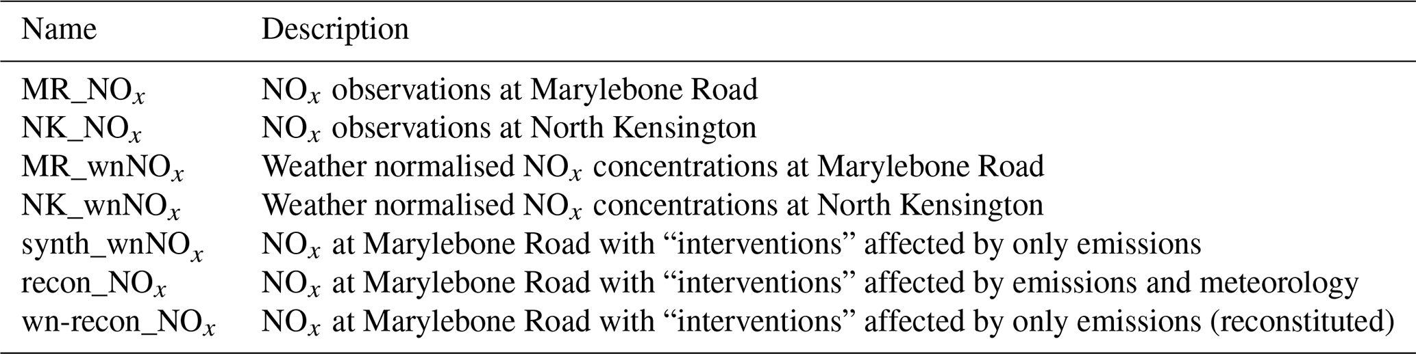
One final step completes the assessment of the approaches to weather normalisation. By reapplying weather normalisation to recon_NO_x, we generated a re-normalised time series (wn-recon_NO_x). In theory, wn-recon_NO_x should closely match, if not exactly replicate, the synth_wnNO_x if the method perfectly isolates emission effects. That is to say, ideally, the weather normalisation operation should “commute” algebraically. Discrepancies between the two normalised time series indicate systematic biases in the weather normalisation process, quantifying over- or underestimation of policy impacts. This comparison provides, to our knowledge, the first evaluation of the accuracy of machine learning weather normalisation approaches in assessing the influence of policy interventions on air quality. The framework described above is generalisable to any policy setting in which the policy impact is masked by weather-like “noise”. Figure 1 shows the schematic diagram for the whole evaluation process, and Table 1 provides a comprehensive list of terminology for NO_x time series used in this study.

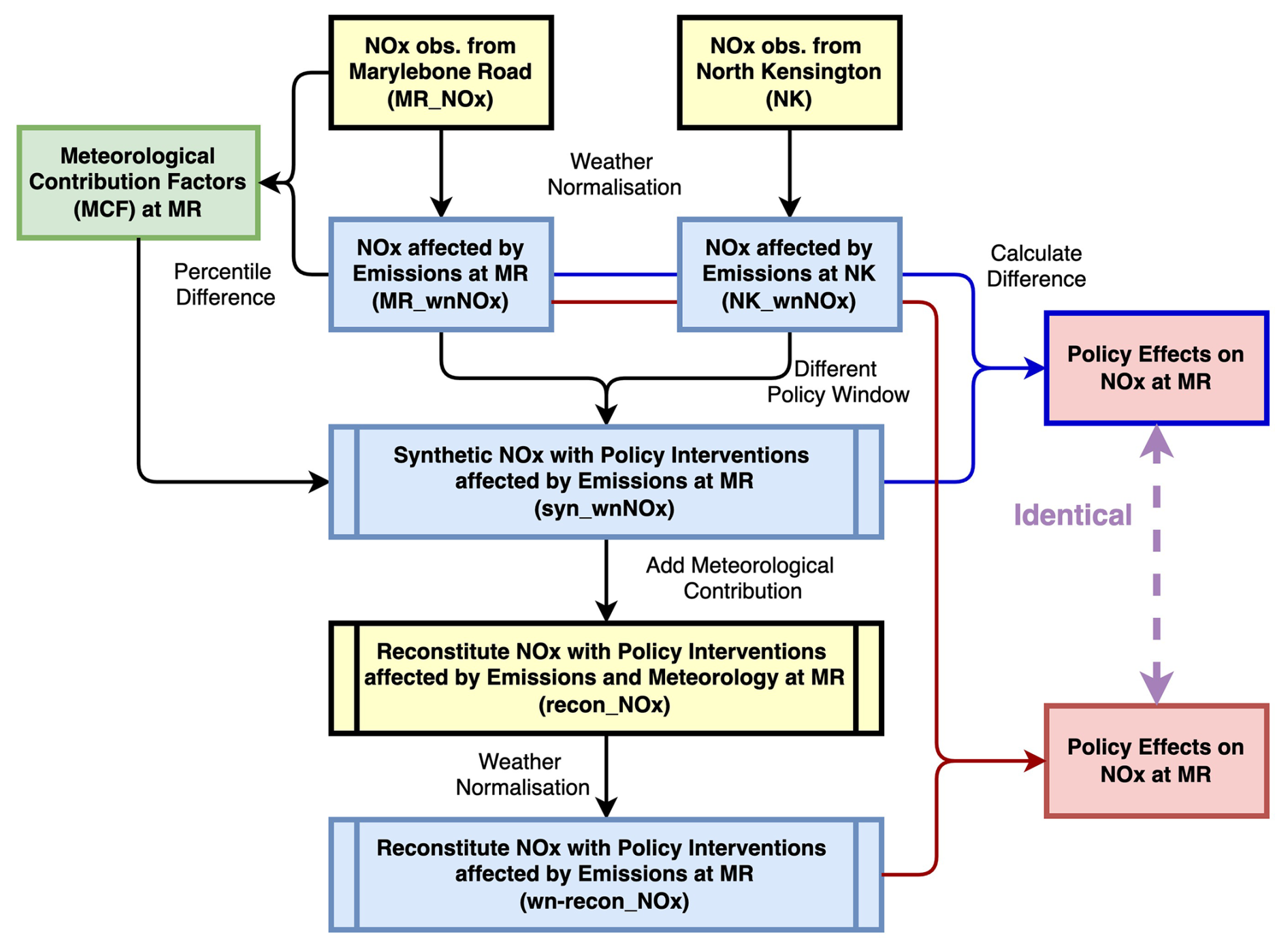
Figure 1 The schematic diagram showing the analytics pipeline to quantify the ability of weather normalisation approaches.

Table 1 A summary of the NO_x timeseries used in the study.

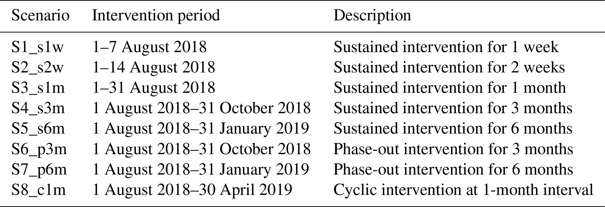
We designed scenarios mimicking diverse real-world policies, including sustained interventions (1 week–6 months), phased reductions (3–6 months), and cyclic interventions (1 month intervals) (Table 2, Fig. S1). These scenarios represent different types of policy interventions and help assess how the weather normalisation methods perform under different temporal patterns of emission changes. Although those sustained 1 week to 6 month cases are idealised “step” emission reductions, we also include phase-out and cyclic patterns specifically to emulate more gradual or heterogeneous real-world responses (e.g., staggered traffic bans or variable industrial curtailments), thereby spanning the continuum from abrupt to progressive interventions. To ensure that our conclusions are not model-specific, we replicated our analysis using different machine learning approaches, including eXtreme Gradient Boosting (XGBoost) and distributed random forest (DRF) models. Performance metrics for these models (Tables S7 and S8) and consistent results across these algorithms (Figs. S11 and S12) indicates the generalizability of our findings. Following the methodological framework described above, we further extend the assessment to the MacLeWN. The weather normalised dataset, the meteorological factors, and the “original” dataset influenced by both emissions and meteorology were presented in Figs. S6–S8, respectively.

Table 2 Overview of air quality intervention durations and strategies for eight test scenarios (S1–S8). In the second part of each scenario name, “s” = sustained intervention, “p” = phased-out intervention, and “c” = cyclic intervention. Intervention durations are for a number (1, 2, 3, or 6) of weeks (“w”), or months (“m”).

2.3.2 Application of Weather Normalisation to COVID-19 Lockdown Data

To further evaluate the performance of the ML-WN and MacLeWN approaches, we applied both techniques to analyse changes in NO_x concentrations during the COVID-19 lockdowns at London Marylebone Road, which will provide a basis to assess emission reductions under abrupt, real-world conditions. Prior studies have used weather normalisation to isolate lockdown effects, but the lack of a definitive “ground truth” for actual pollutant reductions during lockdowns makes it challenging to evaluate these methods absolutely. Our analysis introduces a direct comparison between the ML-WN and MacLeWN under identical scenarios, allowing us to assess their relative performance in isolating lockdown-induced emission changes from meteorological variability.

The lockdown in London was first announced on 23 March, implemented on 26 March, and eased on 23 June 2020 (Davies et al., 2021). The COVID-19 lockdown measures led to an acute drop in NO_x levels at these sites (Lee et al., 2020b). We gathered hourly concentrations of NO_x from 2018 to 2021 for Marylebone from AURN. The corresponding meteorological data (i.e., wd, ws, RH, temp, sp, precip) were obtained from Heathrow Airport. The predictive variables for the machine learning models included temporal variables and meteorological variables as mentioned above. Weather-normalised daily NO_x concentrations around the time of the lockdowns are presented in Fig. S10. Figure S13 shows the variable-importance ranking based on mean absolute SHapley Additive exPlanations (SHAP) values and SHAP contribution plots, whereas Fig. S14 provides partial-dependence plots for the six most influential predictors.

After weather normalisation, we adopted an analytical framework to evaluate the effects of the lockdowns on NO_x concentrations as used in Shi et al. (2021). The baseline period for the lockdown was defined as the 1 month-to-1 week preceding each lockdown (i.e., excluding the final transitional week, Fig. S10), with post-lockdown impacts assessed during the first week of restrictions:

$$\begin{array}{}\text{(9)}& {\displaystyle }\mathrm{\Delta }{C}_{{\mathrm{NO}}_x,t}=C_{{\mathrm{NO}}_x,t}-\stackrel{\mathrm{‾}}{C_{{\mathrm{NO}}_x}}{\mathrm{|}}_t\text{(10)}& {\displaystyle }{P}_{{\mathrm{NO}}_x,t}=\mathrm{100}\mathit{\%}\times {\displaystyle \frac{\mathrm{\Delta }{C}_{{\mathrm{NO}}_x,t}}{\stackrel{\mathrm{‾}}{C_{{\mathrm{NO}}_x}}}}\end{array}$$

$\stackrel{\mathrm{‾}}{C_{{\mathrm{NO}}_x}}{\mathrm{|}}_t$ represents the average value of NO_x at a given hour during the baseline period, $C_{{\mathrm{NO}}_x,t}$ represents the NO_x concentrations at a time t during the first week, 1 month, or 3 months after the lockdown, $\mathrm{\Delta }{C}_{{\mathrm{NO}}_x,t}$ and $P_{{\mathrm{NO}}_x,t}$ represent the absolute and percentage changes in NO_x concentrations in 2020, respectively.

Emissions within a given year are subject to temporal trends, such as gradual policy shifts, economic fluctuations, or seasonal patterns like reduced heating fuel use during winter-to-spring transitions. These trends, unrelated to lockdown measures, risk conflating long-term or cyclical changes with short-term lockdown effects. To account for this, we detrended the data by comparing 2020 NO_x concentrations against the averaged values from the corresponding periods in 2018 and 2019. This 2-year baseline (i.e., for “trend”) was selected to mitigate the influence of interannual variability. The lockdown-driven changes in NO_x concentration ($C_{{\mathrm{NO}}_x,t}^{\ast }$) and their percentage equivalents ($\mathrm{\Delta }{P}_{{\mathrm{NO}}_x,t}^{\ast }$) were calculated as:

$$\begin{array}{}\text{(11)}& {\displaystyle }\mathrm{\Delta }{C}_{{\mathrm{NO}}_x,t}^{\ast }=\mathrm{\Delta }{C}_{{\mathrm{NO}}_x,t}-\mathrm{\Delta }{C}_{{\mathrm{NO}}_x,t}^{\mathrm{2018}\text{–}\mathrm{2019}}\text{(12)}& {\displaystyle }\mathrm{\Delta }{P}_{{\mathrm{NO}}_x,t}^{\ast }=\mathrm{100}\mathit{\%}\times {\displaystyle \frac{\mathrm{\Delta }{C}_{{\mathrm{NO}}_x,t}^{\ast }}{\stackrel{\mathrm{‾}}{C_{{\mathrm{NO}}_x}}}}\end{array}$$

3 Results

3.1 Comparison of two approaches in the theoretical framework

Figure 2a presents a comparative analysis of NO_x reductions, contrasting the “actual” intervention outcomes (red bars) with the predicted simulations derived from the ML-WN approach (blue bars) across eight idealised intervention scenarios (S1–S8, Table 1). The consistent discrepancies between the red and blue bars indicate that the ML-WN approach systematically underestimates the effectiveness of policy interventions, particularly in short-term scenarios. This underestimation occurs because the ML-WN method averages each time-step over meteorological samples drawn from the whole historical record; such averaging sometimes could be unrealistic that “blurs” the sharp drop introduced by the intervention, which is discussed further in the discussion. This underestimation has not been reported before, primarily because it is challenging to detect when comparing a single time series with and without weather normalisation. Importantly, the same qualitative pattern (i.e., MacLeWN > ML-WN) holds also for both phase-out and cyclic scenarios, showing robustness even when the rebound signal after the intervention is not instantaneous.

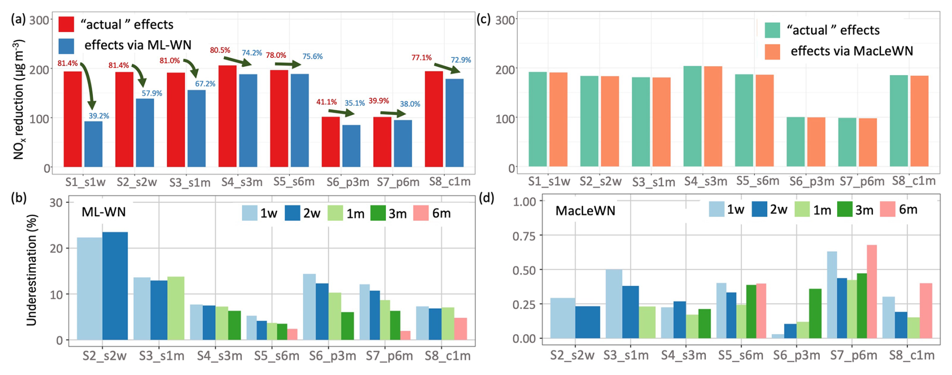
Figure 2 Average intervention effects on NO_x concentrations at Marylebone Road (MR) under different scenarios, including sustained interventions lasting from 1 week (S1_s1w) to 6 months (S1_s6m), phased-out interventions over three (S6_p3m) to 6 months (S7_p6m), and cyclic interventions with a 1 month frequency (S8_c1m). (a, c) The red and green bars represent the “actual” intervention effects based on the theoretical evaluation framework, while the difference between red bars and effects estimated by weather normalisation approaches indicates the extent of underestimation. (b, d) The bars represent underestimated average intervention effects at different time periods as a percentage. Note the different y-axis ranges in panels (b) and (d).

Our results show that the underestimation is particularly significant for short-term interventions. For example, for the 1 week sustained intervention (S1_s1w), the ML-WN approach underestimates the policy effects by 101.1 µg m⁻³, corresponding to a 42.2 % discrepancy. Such substantial underestimations could lead to significant misjudgements of the short-term air quality improvements and the resultant health impacts of air pollutants (Meng et al., 2021). As the duration of the intervention increases to 2 weeks (S2_s2w) and 1 month (S3_s1m), the underestimation decreases to 54 µg m⁻³ (23.5 %) and 35.2 µg m⁻³ (13.8 %), respectively. This pattern continues for policy interventions sustained over longer periods, with the underestimation further decreasing to 17.9 µg m⁻³ (6.3 %) for 3 months (S4_s3m) and 7.9 µg m⁻³ (less than 3 %) for 6 months (S5_s6m). These results indicate that the ML-WN method becomes more accurate over longer intervention periods, possibly because the model adjusts to new emission patterns over time.

Furthermore, the degree of underestimation is more associated with the duration of policy interventions than with the type of policy (i.e., sustained, phased out, or cyclic). For example, both sustained and phased-out policies spanning three and 6 months show similar levels of underestimation. In contrast, cyclic policies with 1 month intervals (S9_c1m) result in an underestimation of 16 µg m⁻³ (4.8 %), which is smaller compared to the underestimations observed in other policy types. Although these discrepancies are smaller compared to short-term interventions, they are still significant when considering long-term average threshold values for public health impacts (Faustini et al., 2014).

Figure 2b illustrates the time-dependent discrepancies in the underestimation of policy impacts on NO_x concentrations, as estimated by the ML-WN approach under different intervention scenarios. For example, S6_p3m scenario, representing a phased-out policy implemented over 3 months, has an overall underestimation of 16.6 µg m⁻³ (6 %, light green bar) but exhibits a 38.1 µg m⁻³ (14.4 %) underestimation in the first week (light blue bar). These results show that, for policies with immediate effects (i.e., sustained policies), the initial underestimation of their efficacy by the ML-WN approach is most pronounced in the early stages but diminishes over time. The extent of this underestimation is inversely related to the duration of the policy implementation. As the duration of the policy extends beyond 1 month, the discrepancy between the anticipated and “actual” impact in the initial stages decreases significantly.

Specifically, during the first week after policy implementation, the underestimation of NO_x reduction is 51.9 µg m⁻³ (13.6 %) for a 2 week policy (S2_s2w), diminishing to 13.4 µg m⁻³ (5.3 %) for a policy sustained over 6 months (S5_s6m). Similarly, the net underestimations of NO_x reduction after 2 weeks are 54 µg m⁻³ (23.5 %), 33.3 µg m⁻³ (13 %), 19.4 µg m⁻³ (7.5 %), and 11 µg m⁻³ (4.2 %) for S2_s2w, S3_s1m, S4_s3m, and S5_s6m, respectively. In contrast, phased-out policies, which gradually reduce interventions over time, present a different pattern. Although their cumulative effects align with those of sustained policies, the initial weeks show a marked underestimation of impact. Figure 2b shows that a 3 month phased-out policy (S6_p3m) results in an overall underestimation of 16.6 µg m⁻³ (6.0 %), and a 6 month policy (S7_p6m) at 6.4 µg m⁻³ (1.9 %). However, the first-week underestimations are 38.1 µg m⁻³ (14.4 %) and 29.9 µg m⁻³ (12.1 %), respectively. Similarly, the cyclic policy (S8_c1m) shows a 7.3 % underestimation in the first week, which is somewhat higher than the overall underestimation observed over the 6 month duration (4.8 %).

By employing the updated machine learning approach (MacLeWN), these underestimations were mitigated, as shown in Fig. 2c and d. The results show a strong agreement between the “known” NO_x reductions resulting from idealised policy interventions and those simulated by the MacLeWN approach. While minor discrepancies are observed in the time-dependent analysis in Fig. 2d, these variations are consistently small, each remaining below 1 %, and showing improvements of greater than an order of magnitude, often by a factor of 20 to 50, compared to the underestimations observed with the ML-WN approach as in Fig. 2b. Further details are provided in Tables S4 and S5, and Figs. S5 and S9.

3.2 Comparison of two approaches in the lockdown scenario

Figure 3 provides the impact of lockdown measures on NO_x concentrations near the roadside at London Marylebone Road air quality monitoring site. NO_x reductions were assessed over 1 week, 1 month, and 3 months after the lockdown implementation by using the direct observations (blue bars), the ML−WN (purple bars), and the MacLeWN (green bars) approaches, respectively. The bars depict the average detrended concentrations changes at the MR site over the policy implementation period following lockdown, and the error bars denote the standard error of the mean. For 1 week lockdown effects, the observed NO_x decreased from 153.9 to 27.5 µg m⁻³ (−82.1 %); the ML-WN estimates a decrease from 158.1 to 76.0 µg m⁻³ (−51.9 %); and the MacLeWN estimates a decrease from 153.2 to 47.7 µg m⁻³ (−68.9 %). In the case of 1 month intervention effect, direct observations indicate a NO_x decrease from 134.3 to 43.6 µg m⁻³ (−67.5 %), the ML-WN indicates a decrease from 150.9 to 71.9 µg m⁻³ (−52.3 %), and the MacLeWN points to a −62.3 % reduction from 141.3 to 53.2 µg m⁻³. For 3 month lockdown effects, NO_x reductions through the observations, the ML-WN, and the MacLeWN are −58.1 ± 6.6 µg m⁻³ (−53.7 %), −71.9 ± 6.0 µg m⁻³ (−51.3 %), and −72.8 ± 8.1 µg m⁻³ (−57.4 %), respectively (Table 3). These results are consistent with the theoretical evaluation presented above, as the ML-WN approach estimates around 17 % lower policy impact compared to the MacLeWN approach but decrease with longer policy implementation time (i.e., about 10 % lower for 1 month lockdown and is insignificant for 3 month effect).

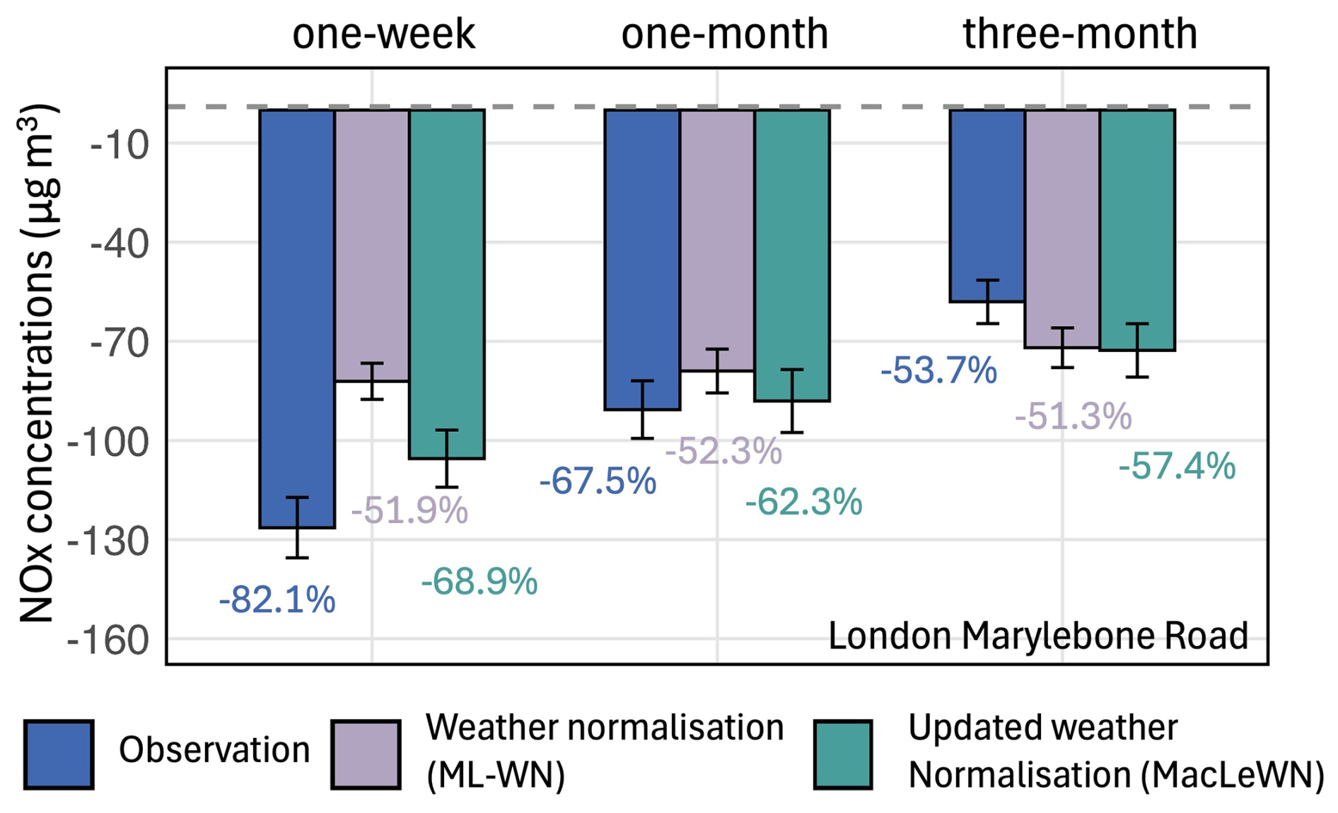
Figure 3 Intercomparison of detrended NO_x concentration changes at London Marylebone Road using direct observations, the weather normalisation (ML-WN), and the updated weather normalisation (MacLeWN) approaches. The bar graphs in the panel show concentration changes ($C_p^{\ast }$) in NO_x over 1 week, 1 month, and 3 months average following lockdown implementation, respectively. Each graph contrasts the raw observation data (dark blue), ML-WN changes (light purple), and MacLeWN changes (dark green). For each bar, the average percentage changes ($P_{\mathrm{p}}^{\ast }$) has been calculated and presented.

Table 3 Absolute and percentile COVID-19 lockdown impacts on NO_x concentrations at London Marylebone Road, analysed through direct observations, the weather normalisation (ML-WN), and the refined weather normalisation (MacLeWN) after measures implemented 1 week, 1 month, and 3 months, respectively.

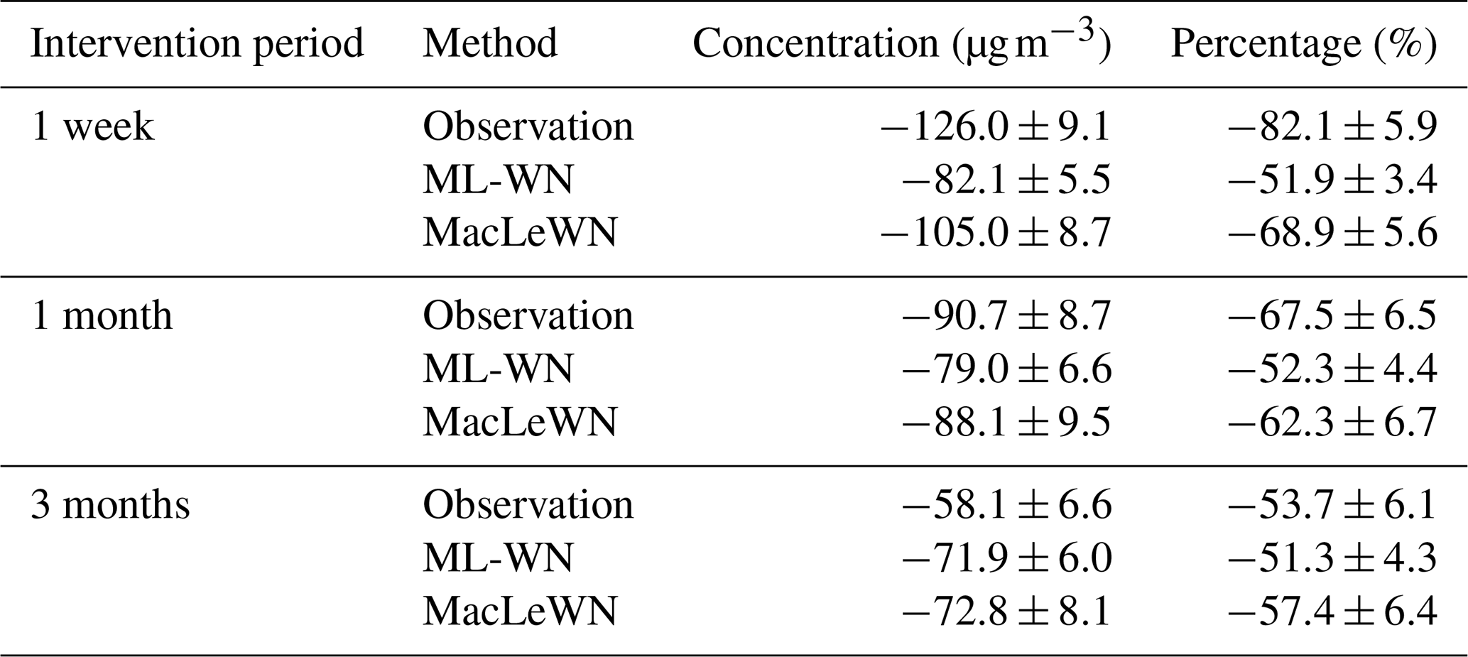
Note: In each case, the data are detrended following the method in Sect. 2.3.2; the uncertainties are expressed as the standard error.

4 Discussion

Accurately assessing the impact of policy interventions on air quality remains a critical challenge, as meteorological variability often obscures the signal of emission-driven changes. While machine learning-based weather normalisation (ML-WN) has emerged as a powerful tool to disentangle these effects, our findings reveal its limitations in evaluating short-term interventions. For example, we showed underestimations of up to 42 % in the quantified effectiveness of 1 week policies (Figs. 2, S4 and S5), indicating that the ML-WN may not fully capture abrupt, non-linear changes in emissions following rapid policy implementation. This discrepancy highlights a fundamental tension: while ML-WN works well at isolating long-term meteorological influences, its reliance on historical patterns may render it less sensitive to transient disruptions in emission regimes.

The root of these uncertainties lies in the interplay between model architecture, variable interdependencies, and real-world complexity. The accuracy of ML-WN depends on the predictive robustness of its underlying algorithms, which must generalize beyond training data to capture sudden shifts in emissions. However, temporal variables (e.g., hour, day, season) and meteorological parameters (e.g., temperature, wind speed) are deeply intertwined in environmental systems. Temporal indicators generally act as proxies for human activity-driven emissions, yet they correlate systematically with meteorological cycles, such as solar radiation peaks at midday, atmospheric stability varies diurnally, and seasonal weather patterns drive recurring emission scenarios (e.g., heating demand in winter). These collinearities create a “proxy trap”, where models may conflate emission-driven trends with weather-driven fluctuations. Tree-based ensembles, while resilient to multicollinearity in prediction tasks, face interpretability challenges: variable importance metrics become unstable when predictors are correlated, splitting attribution across redundant features. Consequently, the “brute force” resampling central to ML-WN (i.e., simulating counterfactual meteorological conditions across time), may inadvertently dilute the signal of abrupt policy impacts, particularly when interventions disrupt established correlations between time and emissions.

Further limitations arise from the fidelity of input data and the physical plausibility of resampled scenarios (Kilkenny and Robinson, 2018). ML-WN assumes meteorological variables can be independently perturbed, yet real-world weather systems exhibit tightly coupled dynamics (e.g., temperature-humidity relationships, land-sea breeze cycles). Resampling risks generating unphysical combinations, for instance, applying wintertime temperature inversions to summer datasets could distort ozone chemistry or particulate dispersion pathways (Vu et al., 2019). Moreover, meteorological conditions absent during the model training phase can compromise predictive accuracy, especially in urban areas subject to complex and routine meteorological events. In coastal urban areas, for instance, diurnal breeze patterns regulate pollution advection (Geddes et al., 2021; Di Bernardino et al., 2021), but models trained on sparse temporal data may fail to resolve these mesoscale processes, leading to biased normalisations.

The application of ML-WN and MacLeWN to COVID-19 lockdown data highlights the practical relevance of our findings. Contrary to the uniform emission cuts assumed in the idealised scenarios, the lockdown produced reductions that were highly variable in both space and time. The observed concentration changes represent a convolution of emission abatement and concurrent meteorological influences. Because percentile NO_x reductions from raw observations consistently exceed those of the weather-normalised estimates generated by ML-WN and MacLeWN, it indicates that the lockdown period coincided with meteorological conditions conducive to pollutant dispersion (Lee et al., 2020a; Acosta-Ramírez and Higham, 2022; Shi et al., 2021). A direct comparison of the two weather-normalised methods shows that their estimates differ by roughly 17 % for a 1 week lockdown, narrowing to 10 % for a 1 month lockdown and 6 % for a 3 month lockdown. These results are consistent with our simulations under idealised conditions (Fig. 2), where ML-WN's smoothing of transient signals could lead to systematic underestimation and MacLeWN shows clear larger policy intervention effects under this real-world policy implementations. Instead of resampling historical weather conditions while keeping the original emission proxies, MacLeWN estimates the influence from weather for each hour by comparing observations relative to pollutant neutral, “normalised emission” baseline, and then it subtracts weather impacts from observations.

From a regulatory aspect, the foregoing analysis indicates that for brief measures (less than 4–6 weeks), MacLeWN scheme should be the preferred approach; for longer programmes (more than 3 months), ML-WN bias falls below 5 %, well within normal error bounds. Policies of intermediate length merit dual reporting with both approaches, giving policymakers a clear span of likely outcomes and sharper grounds for action. It is also important to acknowledge that even the MacLeWN approach may not entirely capture all high-frequency, weather-like variability of air quality. The validity of any weather-normalised scheme ultimately depends on the reliability of the underlying learning model. Reliance on temporal variables as proxies for emissions, rather than direct emission factors, means some meteorological effects correlated with time (e.g., temperature variations throughout the day) may still confound the model; when addressing secondary pollutants such as PM_2.5 or O₃, the predictor set must include proxies for precursor abundance so that the algorithm can disentangle chemistry–meteorology coupling rather than mis-assign chemical production to “weather” effects. Model performance also remains context-dependent. In tropical or arid areas, the weak seasonality, deep convection, and episodic dust plumes can shorten meteorological autocorrelation and undermine resampling stability, while mountainous terrain introduces local circulations that are seldom captured by single-station inputs. Nonetheless, MacLeWN represents an improvement in assessing the immediate impacts of short-term policy interventions.

5 Conclusions

In this work, our logical analysis shows that the widely used machine-learning weather normalisation (ML-WN) approach could markedly underestimate the immediate benefits of short-term air quality interventions. Across eight idealised but plausible NO_x-reduction scenarios at London's Marylebone Road, the ML-WN framework missed up to 42 % of the 1 week reduction signal and still understated 1 month effects by ∼ 14 %. We proposed a refined weather normalisation method MacLeWN that significantly reduced such biases, bringing re-normalised concentrations into near-identity with the known synthetic truth. When applied to the real-world COVID-19 lockdown on Marylebone Road, London, the ML-WN tended to yield more conservative estimates compared to MacLeWN, particularly for shorter intervention periods at 1 week (∼ 52 % vs. 69 %). This further highlight that the ML-WN smooths away a substantial fraction of the abrupt emission signal.

While the proposed MacLeWN refinement is self-consistent, and potentially reduces underestimation biases in weather normalization, its reliability remains contingent on the explainability of the underlying machine learning models, necessitating cautious interpretation and continuous evaluation. Importantly, improving model transparency can increase confidence in the assessments provided by machine learning. The performance of machine learning models is directly influenced by the quality and relevance of their input variables (Geiger et al., 2020). Incorporating specific, causally relevant predictive variables – such as traffic counts, fleet compositions, and industrial emission data – can improve both model performance and explainability in air quality simulations. Strategies such as assessing multicollinearity using statistical measures like the Variance Inflation Factor (Thompson et al., 2017), applying dimensionality reduction techniques like Principal Component Analysis (Abdi and Williams, 2010), employing alternative importance measures less sensitive to correlation (e.g., permutation-based methods) (Mi et al., 2021), and using model interpretation tools like partial dependence plots (Greenwell, 2017) and SHapley Additive exPlanations (SHAP) values (Gebreyesus et al., 2023) can be employed. These approaches not only improve predictive accuracy but also enhance model robustness and interpretation, making them more reliable tools for evaluating the effectiveness of environmental policies.

Our findings have significant implications for the evaluation of air quality interventions and formulation of environmental policies. Although the underestimation of pollutant reductions by the ML-WN decreases for interventions sustained over 3 months (< 5 %), the potential to overlook immediate benefits remains a concern, especially for short-term and emergency measures that necessitate precise evaluation for timely public health responses. Examples include policies implemented during events like sports gatherings and festivals (Yao et al., 2019; Singh et al., 2010; Andrews, 2008), emergency responses to air pollution episode (Tian et al., 2019), and abrupt air pollution incidents such as fireworks displays, industrial accidents, volcanic eruptions, warfare, and wildfires. Additionally, significant social changes, such as those observed during the COVID-19 pandemic, have demonstrated how rapid shifts in human activity can affect air quality (Zangari et al., 2020; Gualtieri et al., 2020). Underestimation of benefits may lead to underappreciation of policy measures and improper resource allocation, affecting public confidence and future support for environmental initiatives. Moreover, weather normalisation errors propagate into downstream methodologies like the Synthetic Control Method (SCM), which constructs a synthetic treated unit from a combination of control units that were not subjected to the intervention, aiming to estimate how pollutant concentrations would have evolved in the absence of the policy (Mork et al., 2024). SCM Controlling for meteorological factors is important to isolate the effects of the intervention from natural weather variations that influence pollutant behaviour and dispersion (Dai et al., 2024). However, if the weather normalisation method introduces inherent underestimation bias in the treated unit, it would lead to a smaller apparent difference between the treated and synthetic control units, thereby skewing the assessment of the true effect of policy interventions (Ben-Michael et al., 2021; Xu, 2017).