A diagnostic intercomparison of modeled ozone dry deposition over North America and Europe using AQMEII4 regional-scale simulations

This study analyzes ozone (O₃) dry deposition fluxes and velocities (V_d) from 12 regional-scale simulations that were performed over North America and Europe in Phase 4 of the Air Quality Model Evaluation International Initiative (AQMEII4). AQMEII4 collected grid-aggregated and land-use-specific (LU-specific) O₃ V_d and effective conductances and fluxes for the four major dry deposition pathways. Consistent with recent findings in the AQMEII4 point model intercomparison study, analysis of the grid-aggregated fields shows that grid models with a similar V_d can exhibit significant differences in the absolute and relative contributions of the different depositional pathways. Analysis of LU-specific V_d and effective conductances reveals a general increase in model spread compared to grid-aggregated values. This indicates that an analysis of only grid-aggregated deposition diagnostics can mask process-specific differences that exist between schemes. An analysis of AQMEII4 LU distributions across models revealed substantial differences in the spatial patterns and abundance of certain LU categories over both domains, especially for non-forest partially vegetated categories such as agricultural areas, shrubland, and grassland. We demonstrate that these differences can significantly contribute to or even drive differences in LU-specific dry deposition fluxes which can increase the variability in model predictions of ozone. Two recommendations for future deposition-focused modeling studies emerging from the AQMEII4 analyses presented here are to (1) routinely generate diagnostic outputs to advance a process-based understanding of modeled deposition and support impact analyses and (2) recognize the importance of documenting and analyzing the representation of LU across models and work towards harmonizing this aspect when using air quality grid models and model ensembles for deposition analyses.

1 Introduction

Dry deposition to the surface is one of the largest sinks in the budget of tropospheric ozone (O₃) (Wild, 2007) and can be a key contributor to O₃ variability (Clifton et al., 2020a; Lin et al., 2020; Baublitz et al., 2020). As summarized in Hardacre et al. (2015) based on previous global modeling studies (Stevenson et al., 2006; Wild, 2007; Ganzeveld et al., 2009; Young et al., 2013), the magnitude of this sink has been estimated to be on the order of 1000 Tg yr⁻¹, with about two-thirds of the dry deposition flux occurring over land and the remaining one-third occurring over oceans. Most global and regional chemistry transport models (CTMs) employ resistance frameworks to represent O₃ dry deposition, such as the frameworks introduced in Wesely (1989) and Zhang et al. (2003). In these frameworks, dry deposition fluxes are represented as the product of the O₃ mixing ratio and a deposition velocity (V_d), which in turn is represented as a combination of process-specific resistances acting in parallel or in series to impede the transfer of mass to the surface. However, the implementation of these resistance frameworks can differ significantly across models, especially with respect to representing the surface resistance and its split between the stomatal and non-stomatal components (Hardacre et al., 2015; Wu et al., 2018; Wong et al., 2019; Clifton et al., 2020b, 2023; Galmarini et al., 2021).

The ability of CTMs to provide spatially continuous fields of O₃ mixing ratios, V_d, and dry deposition fluxes has led to their use in numerous studies quantifying ecosystem damages due to O₃ dry deposition. In some studies, ecosystem impacts were calculated using O₃ mixing ratios simulated by global CTMs in conjunction with crop distribution datasets and literature-based concentration–response relationships without explicitly taking into account modeled stomatal dry deposition fluxes (Wang and Mauzerall, 2004; Van Dingenen et al., 2009; Avnery et al., 2011). In a study focused on assessing O₃ dry deposition in global models, Hardacre et al. (2015) analyzed fields of monthly grid-aggregated O₃ dry deposition fluxes from 15 CTMs that had participated in the first Task Force on Hemispheric Transport of Air Pollution (TF HTAP) model intercomparison project (Fiore et al., 2009). Because the native land use (LU) databases used by each model were not available, the study overlaid the modeled fluxes on two independent global LU databases to estimate O₃ fluxes to specific LU types. A similar approach was taken by Schwede et al. (2018) to estimate global nitrogen deposition to forests using deposition fluxes archived from the second TF HTAP model intercomparison (Tan et al., 2018), combining them with a global forest cover dataset independent of the models' internal LU databases. While this approach makes direct use of modeled dry deposition fluxes, potential inconsistencies between the LU datasets used in the CTMs and those used in the post-processing attribution of modeled fluxes to specific ecosystems can introduce uncertainties. Moreover, utilizing archived grid-aggregated deposition fluxes does not account for potential subgrid variations in LU that could have a strong impact on ecosystem-specific deposition. To explore the impacts of such subgrid effects, Schwede et al. (2018) also presented results from the EMEP MSC-W model (Simpson et al., 2012), which employs a mosaic approach to calculate and optionally output V_d and deposition fluxes for each LU present in a grid cell. Results showed that the total global estimate of nitrogen deposition to forest was 12 % higher using forest-specific EMEP fluxes compared to grid-aggregated fluxes and that local fluxes estimated using the two approaches could differ by more than a factor of 2 depending on the LU heterogeneity in a given grid cell (Schwede et al., 2018). A companion paper in this issue (Makar et al., 2025) showed large land-use-dependent variations in deposition fluxes for both sulfur and nitrogen species (particularly for bidirectional fluxes of ammonia gas) and noted that LU databases used for post-processing critical load analysis may also differ from those used in regional models, with harmonization of these databases recommended for future modeling studies.

As discussed above, CTM-based approaches for assessing ecosystem impacts of air pollution can be affected by uncertainties in input datasets (emissions, meteorology, and LU) as well as the representation of a variety of chemical and physical processes. Hardacre et al. (2015) noted that advancing a process-level understanding of how uncertainties and errors in modeled dry deposition contribute to overall CTM error and variability would require the generation of detailed diagnostic model outputs at an hourly resolution, including stomatal and non-stomatal conductances and fluxes at both the grid-aggregated level and for individual LU categories. While a few global modeling studies using individual CTMs have incorporated such diagnostic fields and demonstrated their utility (Paulot et al., 2018; Clifton et al., 2020a) and prior to AQMEII4 this practice was recommended by a recent review (Clifton et al., 2020b), to date it has not been adopted in model intercomparison studies at either the global or regional scale. Partially motivated by this research gap, Phase 4 of the Air Quality Model Evaluation International Initiative (AQMEII4) was designed around complementary grid and single-point modeling activities for a diagnostic intercomparison and evaluation of simulated deposition with a specific focus on dry deposition of gaseous species (Galmarini et al., 2021; Clifton et al., 2023).

Table 1 Model simulations analyzed in this study. See Makar et al. (2025) for additional details on the configuration of each simulation.

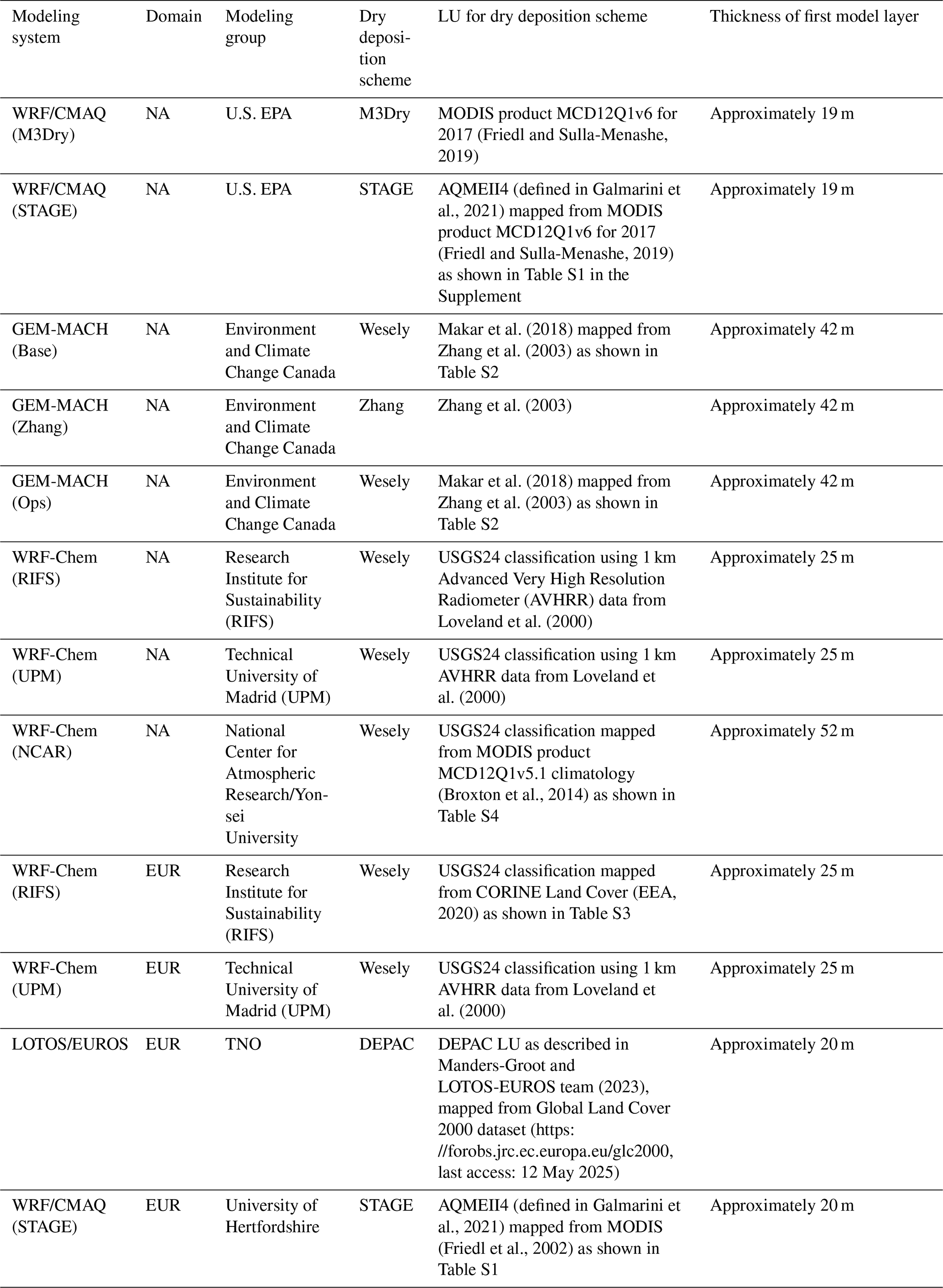
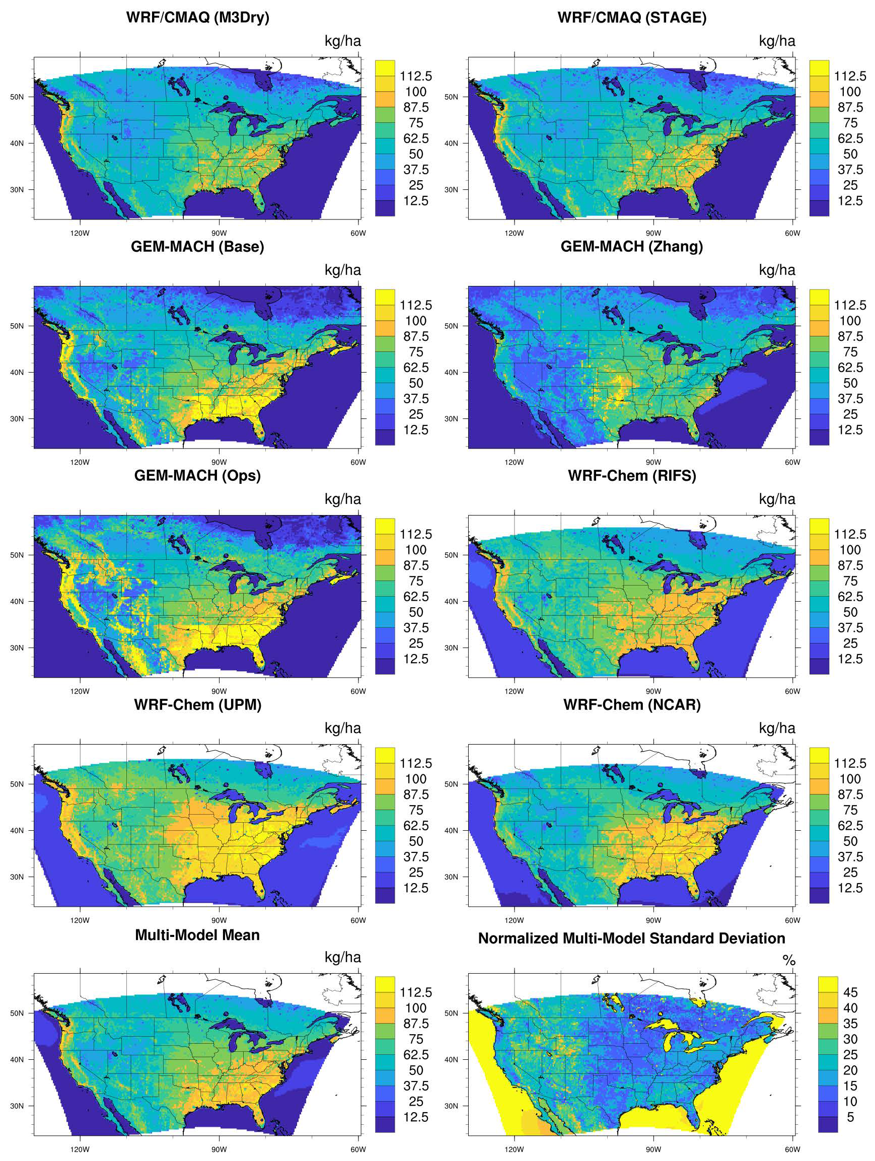
Figure 1 2016 annual total O₃ grid-scale dry deposition fluxes for each model, the multi-model mean, and the normalized multi-model standard deviation over the NA domain. Note that the plots for individual models are not clipped to the domain common to all simulations and show the maximum spatial extent submitted for each model. The multi-model mean and normalized standard deviations are calculated and shown over the common domain.

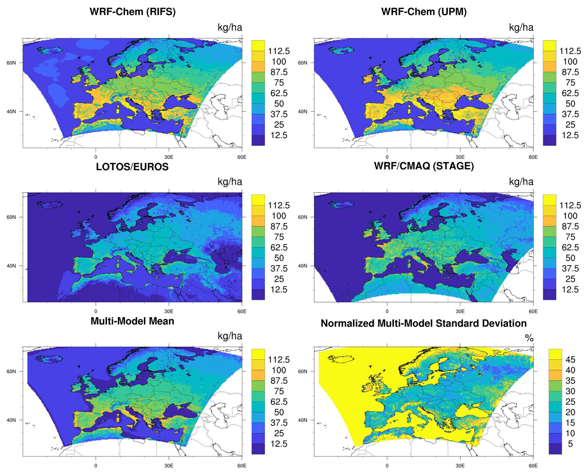
Figure 2 2010 annual total O₃ grid-scale dry deposition fluxes for each model, the multi-model mean, and the normalized multi-model standard deviation over the EUR domain. Note that the plots for individual models are not clipped to the domain common to all simulations and show the maximum spatial extent submitted for each model. The multi-model mean and normalized standard deviations are calculated and shown over the common domain.

In this study conducted within the framework of AQMEII4, we apply the diagnostic approaches described in the AQMEII4 technical note (Galmarini et al., 2021) and the paper presenting the evaluation of single-point models at eight long-term O₃ flux measurement sites (Clifton et al., 2023) to the analysis of O₃ dry deposition simulated by the AQMEII4 regional-scale models for analysis domains over North America (NA) and Europe (EUR). The extent of these analysis domains was defined in Galmarini et al. (2021) and is shown in Figs. 1 and 2. Our analysis also leverages the common AQMEII4 LU types defined in Galmarini et al. (2021). As discussed in that study, assigning model native LU types to a common set of 16 AQMEII4 LU types allows for consistent LU-specific comparisons (note that some of the most common LU types, such as evergreen needleleaf forest, are present in all native model LU databases). First, we quantify temporal and spatial variations in estimated O₃ deposition by analyzing different deposition pathways and comparing grid-aggregated vs. AQMEII4 LU-specific diagnostics. We also demonstrate that the LU-specific diagnostics can be used to connect grid model results to the evaluation of single-point models against long-term O₃ flux measurement sites described in Clifton et al. (2023). Next, we assess the impacts of differences in LU between the AQMEII4 grid models on simulated fluxes to different ecosystems. Finally, we discuss the implications of our analyses to O₃ deposition impact studies, particularly impact studies based on datasets from multi-model intercomparison activities, as well as to future model development aimed at improving dry deposition process representation.

2 Datasets

Table 1 lists the participating regional-scale models, the institutions performing the simulations, the continent each simulation was performed for, their dry deposition schemes, the LU classification scheme used in their dry deposition calculations, and the thickness of the first model layer. Detailed descriptions of the model configurations were provided in Makar et al. (2025), while their dry deposition algorithms were documented in Galmarini et al. (2021), Clifton et al. (2023), and Hogrefe et al. (2023). The 16 AQMEII4 LU types to which native LU types were assigned are described in Galmarini et al. (2021) and discussed in detail in Sect. 3.3. An operational and probabilistic evaluation of simulated O₃ mixing ratios against ground-level network observations over NA and EUR is presented in Kioutsioukis et al. (2025).

The analysis in this paper utilizes dry deposition fluxes and the O₃ dry deposition diagnostic variables described in detail in Galmarini et al. (2021) and Clifton et al. (2023), namely O₃ dry deposition velocities (V_d) and effective conductances (Paulot et al., 2018; Clifton et al., 2020a, 2023; Galmarini et al., 2021) for the stomatal, cuticular, soil, and lower canopy surface deposition pathways reported at both the grid-aggregated scale and for each of the 16 AQMEII4 LU categories. Following the general framework introduced in Wesely (1989), all models in this study except WRF/CMAQ (STAGE) calculate V_d as the inverse of the sum of the aerodynamic resistance r_a; the quasi-laminar sublayer resistance r_b; and the surface resistance r_c, which consists of most or all of the parallel deposition pathways listed above but is implemented differently across schemes as documented in Galmarini et al. (2021). The aerodynamic resistance r_a is independent of deposition pathways in all models, and r_b is independent of deposition pathways in all models except WRF/CMAQ (STAGE), which computes different r_b values for stomatal and cuticular vs. soil pathways and therefore includes this term in its pathway-specific r_c calculations. As stated in Galmarini et al. (2021), “an effective conductance is the contribution of a given depositional pathway to the deposition velocity, expressed in the same units as the deposition velocity. The sum of the effective conductances for all deposition pathways is the deposition velocity.” Importantly, Galmarini et al. (2021) noted that the equations used to compute the effective conductances are specific to a given dry deposition scheme and provided these equations for the different AQMEII4 modeling systems in Appendix B. No effective conductances were available for LOTOS/EUROS, but reported grid-aggregated O₃ V_d, deposition fluxes, and LU distributions are included in the analysis.

WRF/CMAQ, GEM-MACH, and LOTOS/EUROS calculate and report V_d and effective conductances at the midpoint of the first model layer, while values in WRF-Chem are calculated as the average over the first layer following McRae et al. (1982). As shown in Table 1, the height of the first model layer varies across models and may therefore affect the comparison of V_d across models. However, only the computation of r_a has a dependency on layer height. When comparing the magnitude of the annual domain-average r_a, r_b, and r_c terms for O₃ across participating models, we find that r_c is typically at least a factor of 10 higher than r_a, suggesting that the effect of different layer heights on our comparison of V_d is relatively minor and that differences in the representation and computation of the parallel surface resistance pathways constituting r_c are the main driver of differences in V_d. In addition, the independence of the different resistances included in the computation r_c (Galmarini et al., 2021; Clifton et al., 2023) on layer height also implies that our analysis of effective conductances to quantify the split between different surface deposition pathways is likely not affected by model-to-model differences in layer heights.

For WRF-Chem (NCAR), LU-specific dry deposition calculations for its native “mixed shrubland/grassland” category were inadvertently mapped to and then reported for the AQMEII4 “savanna” category (along with its native “savanna” category) rather than the intended AQMEII4 “shrubland” category. This inadvertent mapping was corrected for the comparison of LU categories across models but could not be corrected for the analysis of LU-specific V_d and effective conductances. For all models except GEM-MACH (Base) and GEM-MACH (Ops), the spatial fields of LU categories in both the land surface model (LSM) and dry deposition code were time independent and considered the “snow and ice” category to represent permanent snow and ice. For the GEM-MACH (Base) and GEM-MACH (Ops) dry deposition calculations, the LU categories used in the dry deposition calculations and subsequently reported to AQMEII4 were modified from their time-independent LSM values to represent the time-varying effects of transient snow cover through the “snow and ice” category and proportionally reduced the fractions of all other LU categories in the grid cell if snow cover was present. To enable a comparison of these time-dependent LU fractions to the fractions reported by other models, time-independent fractions for GEM-MACH (Base) and GEM-MACH (Ops) were derived by scanning the hourly reported fields and determining the LU fractions in each grid cell when the coverage of the “snow and ice” category reached its annual minimum (zero for the vast majority of grid cells) for that grid cell. This approach allows for the use of LU fractions as a stratification criterion for all models in our analysis while retaining the effects of transient snow cover (represented through separate snow cover fields rather than time-dependent LU fractions in other dry deposition schemes) in the reported dry deposition diagnostics.

As described in Galmarini et al. (2021), each simulation reported gridded fields of V_d and effective conductances as 288 individual values representing monthly median diurnal cycles (24 h times 12 months) at each grid cell for each simulated year. This approach was chosen because reporting and storing these diagnostic fields for all hours in the year would have been logistically impossible, and the selected approach still allows for an analysis of their diurnal and seasonal variations. However, it should be noted that this approach of using monthly median values for individual diagnostics can introduce a temporal mismatch between reported V_d and effective conductance diagnostics, which in turn may cause the sum of the effective conductances on a monthly median basis to differ from monthly median V_d, even though on an hour-by-hour basis their sum equals V_d (Paulot et al., 2018; Clifton et al., 2020a, 2023; Galmarini et al., 2021). Despite this potential for deviations, the sum of the reported effective conductances was found to be within 3.5 % of V_d on an annual domain mean basis for all simulations. The largest deviation (3.5 %) occurred for WRF/CMAQ (M3Dry), for which grid-aggregated V_d was calculated within the model, while effective conductances were estimated through post-processing (Hogrefe et al., 2023). For the remainder of the discussions in this paper, we therefore treat the sum of the monthly median effective conductances as equivalent to V_d.

3 Results

3.1 Grid-aggregated results

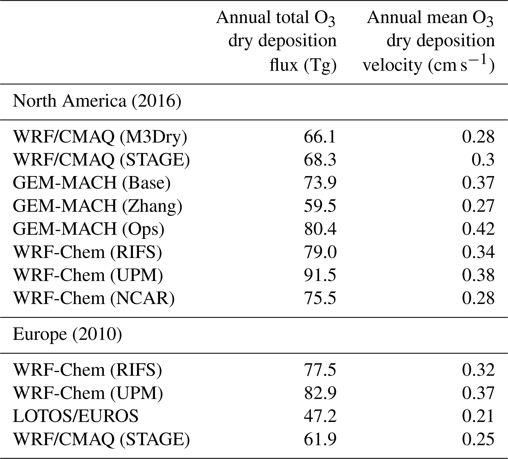
Spatial patterns of these annual deposition fluxes for each model as well as the multi-model mean and normalized standard deviation are displayed in Fig. 1 for the NA domain and Fig. 2 for the EUR domain. Table 2 lists the annual total O₃ dry deposition fluxes estimated by the participating models over both the NA and EUR domains. These totals are calculated over all non-water grid cells that were common to all simulations. The multi-model mean value is 74.3 Tg yr⁻¹ over the NA domain and 67.4 Tg yr⁻¹ over the EUR domain. Individual model estimates range from 59.5 (GEM-MACH (Zhang)) to 91.4 Tg yr⁻¹ (WRF-Chem (UPM)) over the NA domain and from 47.2 Tg yr⁻¹ (LOTOS/EUROS) to 82.9 Tg yr⁻¹ (WRF-Chem (UPM)) over the EUR domain. For context, past global modeling studies reported global annual O₃ deposition totals generally ranging between 800 and 1200 Tg yr⁻¹ (e.g., Hardacre et al., 2015; Stevenson et al., 2006; Wild, 2007; Ganzeveld et al., 2009).

Table 2 Annual total O₃ dry deposition fluxes and annual mean O₃ dry deposition velocities estimated by the participating models over both the NA and EUR domains. These totals are calculated over all non-water grid cells that were common to all simulations. The NA numbers are for 2016, while the EUR numbers are for 2010.

Over the NA domain all models estimate that O₃ deposition is highest over the eastern US as well as along the West Coast, consistent with our expectations that reflect a combination of higher O₃ mixing ratios due to higher O₃ precursor emissions in these regions and higher V_d over areas with higher vegetation density. The pronounced differences in deposition fluxes over the densely vegetated southeastern US between WRF-Chem (UPM) and GEM-MACH (Zhang) suggest that differences in the methodology used to represent deposition to vegetation are a key driver of model spread. The map of the multi-model normalized standard deviation over NA also shows significant spread in deposition to land over the generally more arid regions in the western US, in addition to the spread over the southeastern US. Over the EUR domain, the largest relative spread in deposition to land occurs over northwestern Scandinavia, Ireland, Great Britain, and Türkiye, as well as the Alps and northern Africa. Over both domains, there is a large relative spread in O₃ deposition to water, with generally higher values for WRF-Chem than all other models, but the absolute magnitude of the flux is much smaller than the flux over land.

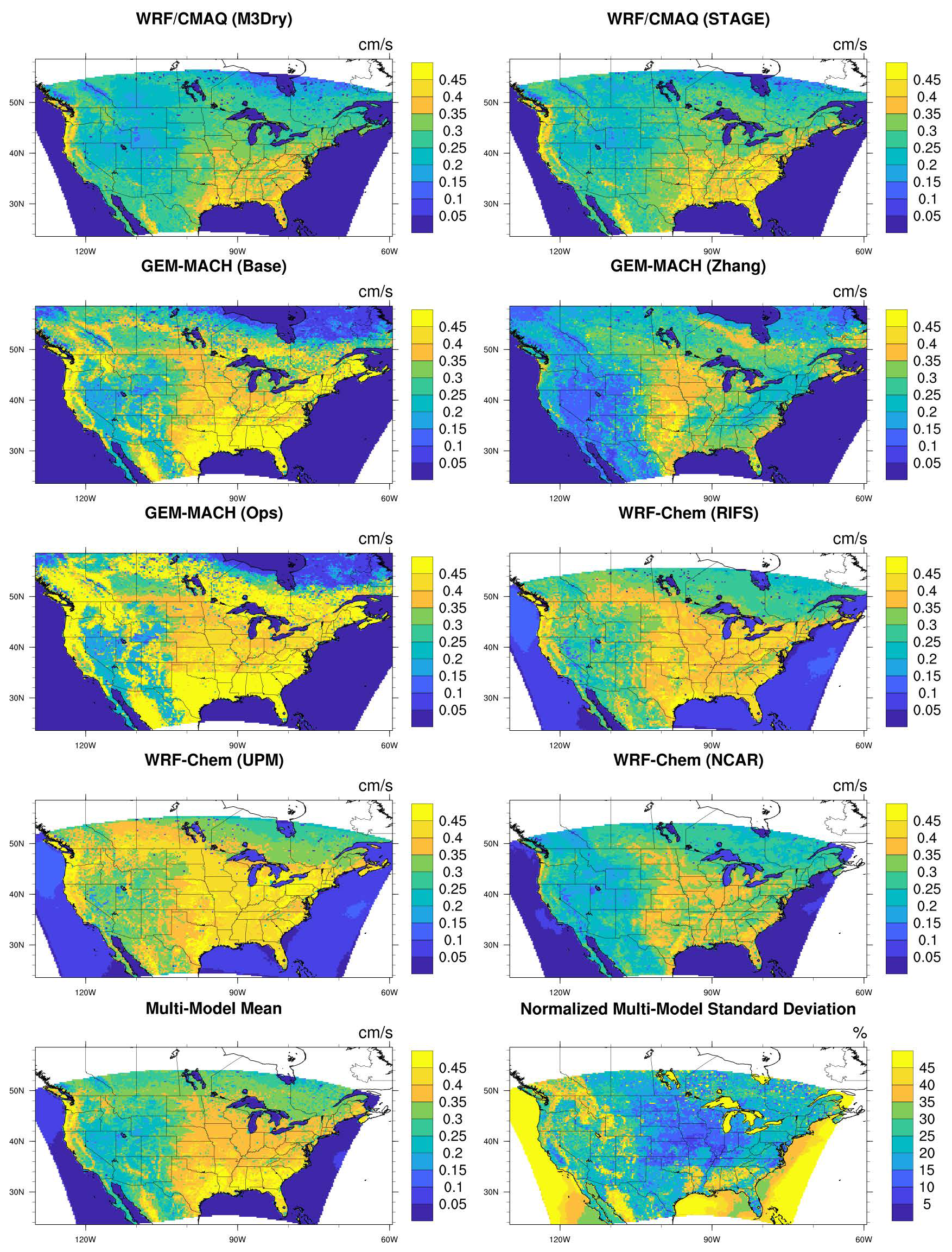
Figure 3 2016 annual mean O₃ grid-scale dry deposition velocities for each model, the multi-model mean, and the normalized multi-model standard deviation over the NA domain. Note that the plots for individual models are not clipped to the domain common to all simulations and show the maximum spatial extent submitted for each model. The multi-model mean and normalized standard deviations are calculated and shown over the common domain.

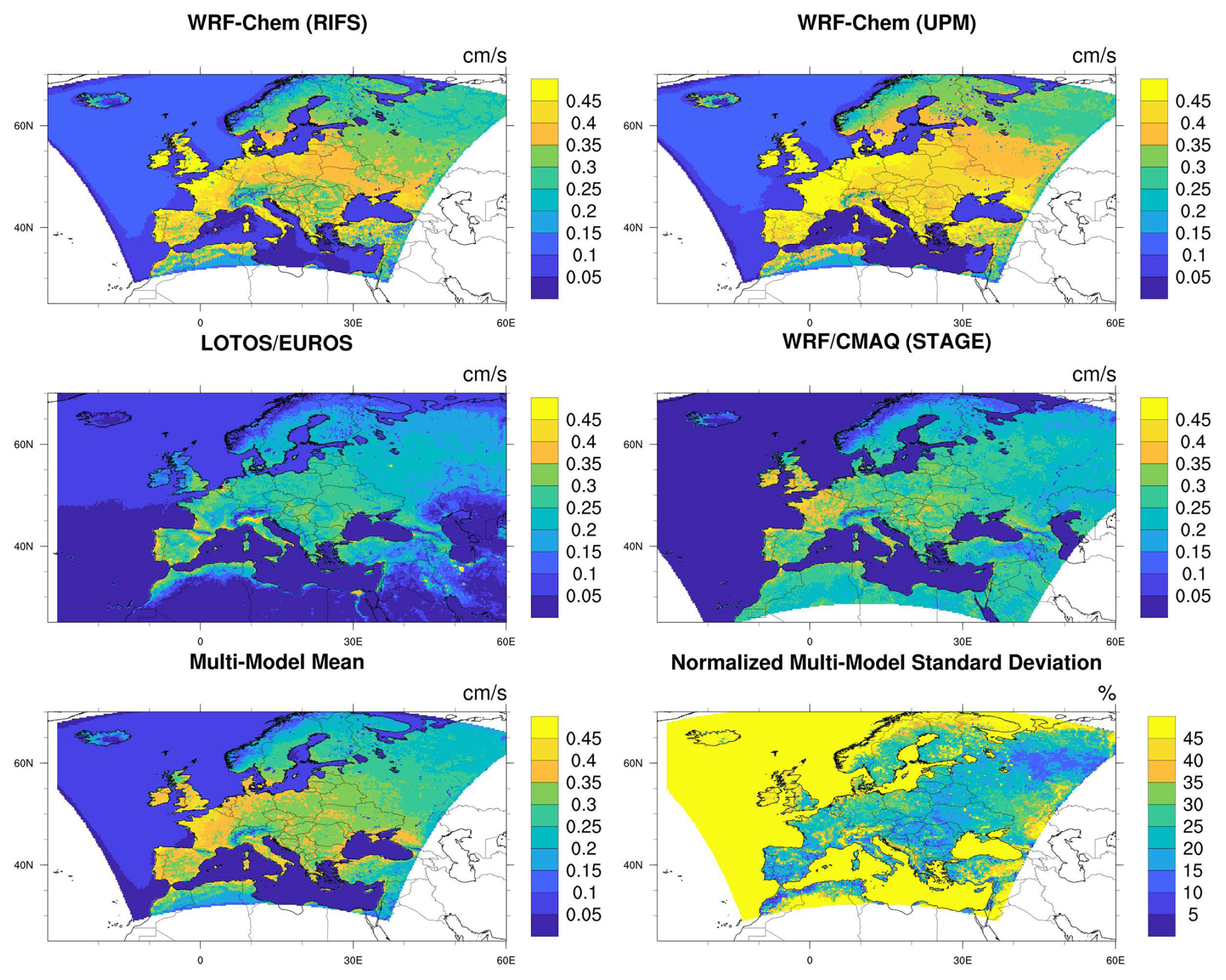
Figure 4 2010 annual mean O₃ grid-scale dry deposition velocities for each model, the multi-model mean, and the normalized multi-model standard deviation over the EUR domain. Note that the plots for individual models are not clipped to the domain common to all simulations and show the maximum spatial extent submitted for each model. The multi-model mean and normalized standard deviations are calculated and shown over the common domain.

To assess the role of variations in simulated V_d on the dry deposition fluxes discussed above, Table 2 includes the annual mean O₃ V_d over both domains alongside the annual total O₃. The relative differences between the annual mean V_d generally match those between the annual total deposition fluxes with only small exceptions (e.g., WRF-Chem (RIFS) has slightly lower V_d but slightly higher dry deposition fluxes than GEM-MACH (Base)). Consistent with the discussion in Sect. 2, the model-to-model differences in V_d shown in Table 2 indeed do not appear to be caused by the different first-layer thicknesses shown in Table 1. Notably, the GEM-MACH (Ops) simulation has the highest V_d, while the GEM-MACH (Zhang) simulation has the lowest V_d despite both simulations having one of the thickest first-layer heights. This is consistent with the notion that the surface resistance r_c (independent of first-layer thickness) rather than the aerodynamic resistance r_a (dependent on first-layer thickness) is generally the limiting factor controlling ozone dry deposition.

Figures 3–4 show the spatial patterns of annual mean V_d for each model and the multi-model mean and normalized standard deviation. While these maps visually confirm the results from Table 2 that GEM-MACH (Ops) has the highest mean V_d and GEM-MACH (Zhang) the lowest mean V_d over the NA domain and WRF-Chem (UPM) has the highest and LOTOS/EUROS the lowest mean V_d over the EUR domain, they also show important spatial differences. For example, both GEM-MACH (Base) and WRF-Chem (UPM) have very similar annual mean V_d when averaged over the entire domain (Table 2), but this agreement in the means masks the generally higher V_d in GEM-MACH (Base) over the southeastern US and the generally lower V_d over the southwestern US compared to WRF-Chem (UPM). The role of differences in surface deposition pathways and LU distributions in causing model-to-model differences in V_d magnitude and patterns is discussed in subsequent sections.

Comparing the model-to-model differences in Figs. 3–4 to those in the corresponding dry deposition flux maps in Figs. 1–2 shows a high level of similarity. For example, the areas over the southeastern US where GEM-MACH (Base) and GEM-MACH (Ops) have larger fluxes than other models coincide with areas where these two simulations also have the highest O₃ V_d. Moreover, the areas with the highest normalized flux standard deviation discussed above for both the NA and EUR domains also show the highest normalized standard deviation for V_d. Despite these general similarities, it is important to note that models may have above-average O₃ fluxes while also having below-average O₃ V_d or that a given model may have areas with a similar V_d but noticeably different dry deposition fluxes, due to the influence of factors other than V_d (e.g., the representation of regional transport and chemistry, the parameterizations for subgrid-scale turbulence, and the location and density of precursor emission sources) on simulated O₃ mixing ratios. Maps of annual mean O₃ for each model as well as the multi-model mean and standard deviation are shown in Figs. S1–S2 in the Supplement, and we refer to Kioutsioukis et al. (2025) for both an operational evaluation of simulated O₃ fields and analyses partitioning variability in these fields to variability in O₃ V_d and other variables such as wind speed and the height of the planetary boundary layer. Makar et al. (2025) showed that WRF-Chem (NCAR) significantly underestimated observed precipitation, and Kioutsioukis et al. (2025) hypothesized that a corresponding underestimation of clouds and overestimation of radiation was the main driver for the large positive ozone bias reported for that model. The above-average O₃ mixing ratio for WRF-Chem (NCAR) shown in Fig. S1 is consistent with this hypothesis and may provide at least a partial explanation for the above-average O₃ flux but below-average O₃ V_d shown for this model in Figs. 1 and 3. As a second example of confounding factors when comparing spatial patterns of O₃ V_d and O₃ fluxes, the GEM-MACH (Ops) panel in Fig. S1 shows generally higher O₃ mixing ratios over the southeastern US vs. parts of the Canadian boreal forest region, consistent with corresponding spatial differences in O₃ fluxes for this model despite similar O₃ V_d in these two regions. The influence of factors other than V_d in shaping spatial O₃ variability is analyzed in more detail in Kioutsioukis et al. (2025). However, despite these potentially confounding influences, the general agreement of both the model rankings for the domain-wide dry deposition fluxes vs. V_d (Table 2) and their spatial patterns (Fig. 1 vs. Fig. 3 and Fig. 2 vs. Fig. 4) confirms the influence of O₃ V_d on deposition fluxes estimated in these regional-scale simulations. This in turn establishes that a diagnostic understanding of simulated O₃ V_d can aid in interpreting model-to-model differences in dry deposition fluxes.

Figures S3 and S4 provide insight into temporal differences in modeled deposition by showing domain-wide deposition fluxes and O₃ V_d calculated for winter vs. summer and daytime vs. nighttime periods for the NA domain. The largest deposition fluxes occur during summer daytime hours, while the lowest deposition fluxes occur during winter nighttime hours, a pattern also present for V_d. Photochemical production of O₃ is also higher in summer than in winter, which will also contribute to higher summertime fluxes. Fluxes during winter daytime hours are generally of the same order of magnitude as fluxes during summer nighttime hours, both times corresponding to low photochemical production or ozone destruction through titration. These figures also suggest that the low annual total deposition value of model GEM-MACH (Zhang) and the high annual total deposition value of model WRF-Chem (UPM) shown in Table 2 were driven by low and high summer daytime flux values, respectively, and/or that other terms such as photochemical production in WRF-Chem (UPM) are enhancing summer ozone concentrations, hence increasing fluxes. While the absolute model-to-model differences are smaller during winter than summer for both fluxes and V_d, the normalized standard deviation is comparable across seasons for both variables (summer daytime flux of 18.2 %; winter daytime flux of 14.5 %; summer nighttime flux of 22.7 %; winter nighttime flux of 22.8 %; summer daytime V_d of 18.6 %; winter daytime V_d of 17.2 %; summer nighttime V_d of 34.2 %; winter nighttime V_d of 28.2 %). During daytime, fluxes and V_d exhibit similar relative spread. The larger nighttime spread in V_d compared to the fluxes suggests that nighttime chemical sinks and/or a smaller ozone reservoir in the shallower nighttime mixing layer may be more important factors controlling O₃ concentrations and hence O₃ deposition fluxes than the magnitude of the deposition velocity itself. However, it should also be noted that Clifton et al. (2020a) found that even small differences in wintertime V_d can have substantial impacts on the tropospheric O₃ budget given the longer chemical lifetime.

Figures 5–6 depict the contributions of the four effective conductance pathways to the annual domain-average V_d for each model over both domains. The total height of the bars for each model closely corresponds to that model's V_d shown in Table 2, within the caveats discussed in Sect. 2. Note that some of these simulations (WRF/CMAQ (M3Dry), WRF/CMAQ (STAGE), and GEM-MACH (Zhang)) do not incorporate a separate lower canopy pathway in their dry deposition schemes and thus only have three deposition pathways in total (Galmarini et al., 2021; Clifton et al., 2023). These figures show that models with a similar V_d (e.g., WRF/CMAQ (M3Dry), GEM-MACH (Zhang), and WRF-Chem (NCAR) over NA) can show significant differences in the absolute and relative contributions of different pathways to V_d. Moreover, these figures also demonstrate that effective conductances allow for an attribution of model differences in V_d to specific processes. For example, GEM-MACH (Base), GEM-MACH (Ops), and WRF-Chem (RIFS) all have similar soil and lower canopy effective conductances, revealing that the differences in V_d between these simulations stem from differences in the cuticular and, to a lesser extent, stomatal pathways. Specifically, both GEM-MACH (Base) and GEM-MACH (Ops) have a higher cuticular effective conductance than WRF-Chem (RIFS). For the two CMAQ simulations over NA, Fig. 5 confirms the generally larger contributions from the stomatal and cuticular pathways for WRF/CMAQ (M3Dry) and the generally larger contribution from the soil pathway for WRF/CMAQ (STAGE) that was reported in Hogrefe et al. (2023). Comparing GEM-MACH (Base) with GEM-MACH (Zhang) shows lower contributions from the soil and stomatal pathways for the latter, which also does not include a separate lower canopy pathway.

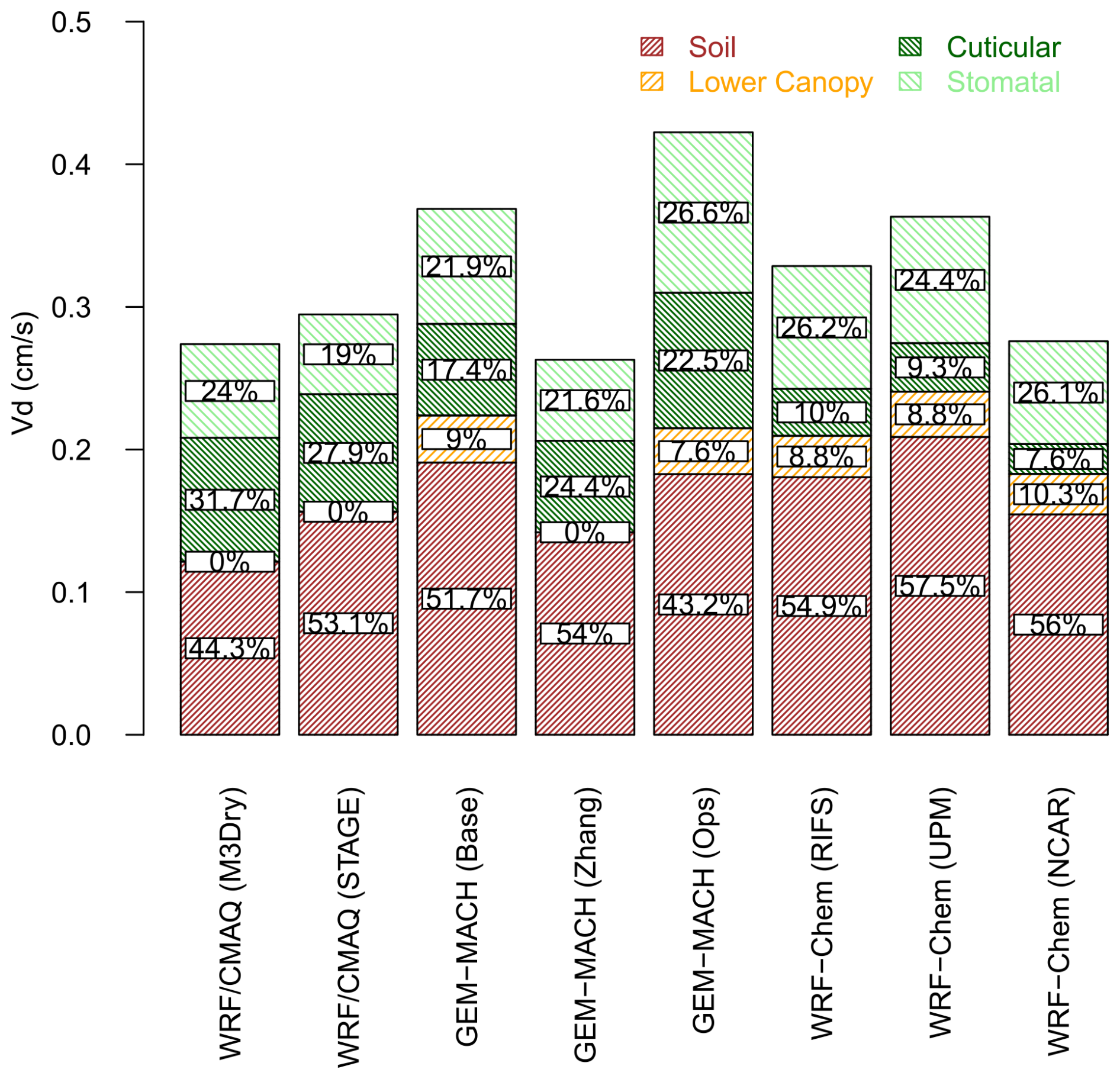
Figure 5 Annual domain-average grid-scale effective conductances and ozone deposition velocities for 2016 over the NA domain. Averages were calculated over all non-water grid cells in the portion of the analysis domain shared by all model simulations.

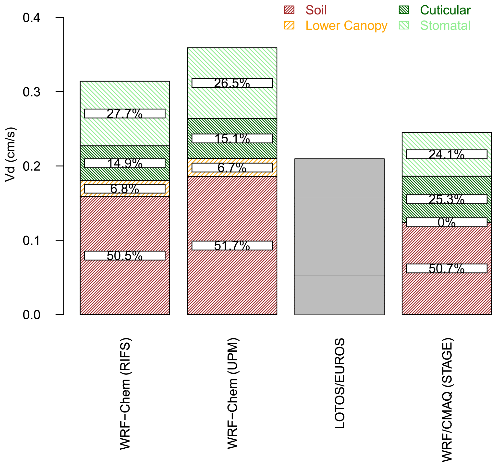
Figure 6 Annual domain-average grid-scale effective conductances and ozone deposition velocities for 2010 over the EUR domain. Averages were calculated over all non-water grid cells in the portion of the analysis domain shared by all model simulations. The bar for LOTOS/EUROS shows only the deposition velocity since no effective conductances were reported.

Comparing the two GEM-MACH simulations with the same dry deposition scheme, GEM-MACH (Base) and GEM-MACH (Ops), reveals that differences other than the dry deposition scheme that exist between these simulations (e.g., meteorology and leaf area index (LAI)) have a noticeable impact on the magnitude of the cuticular and stomatal pathways. It should be noted that both GEM-MACH (Base) and GEM-MACH (Ops) are coupled models with chemistry residing within a weather forecast model; however, GEM-MACH (Base) is “fully coupled”, i.e., includes aerosol direct and indirect feedbacks on the predicted meteorology. GEM-MACH (Base) also includes several other parameterizations affecting chemical transport as noted above. The difference in the strength of the cuticle and stomatal conductances between these two models thus reflects differences in the forecasted meteorology, in turn influencing the deposition velocity components.

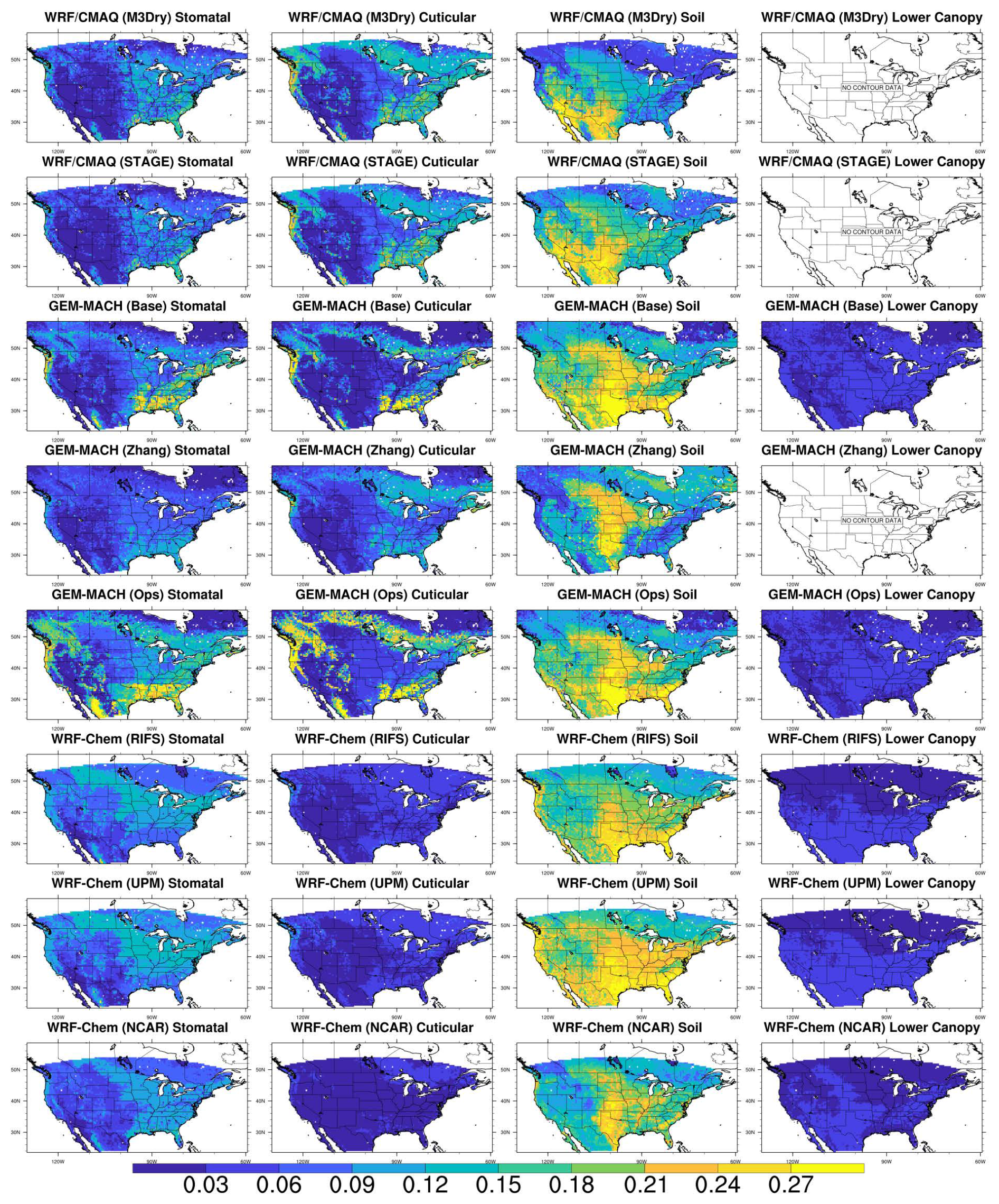
Figure 7 Absolute grid-scale ozone effective conductances (cm s⁻¹), averaged over the entire year. Results are for the NA domain during 2016. Note that these maps are not clipped to the domain common to all simulations and show the maximum spatial extent of non-water cells submitted for each model.

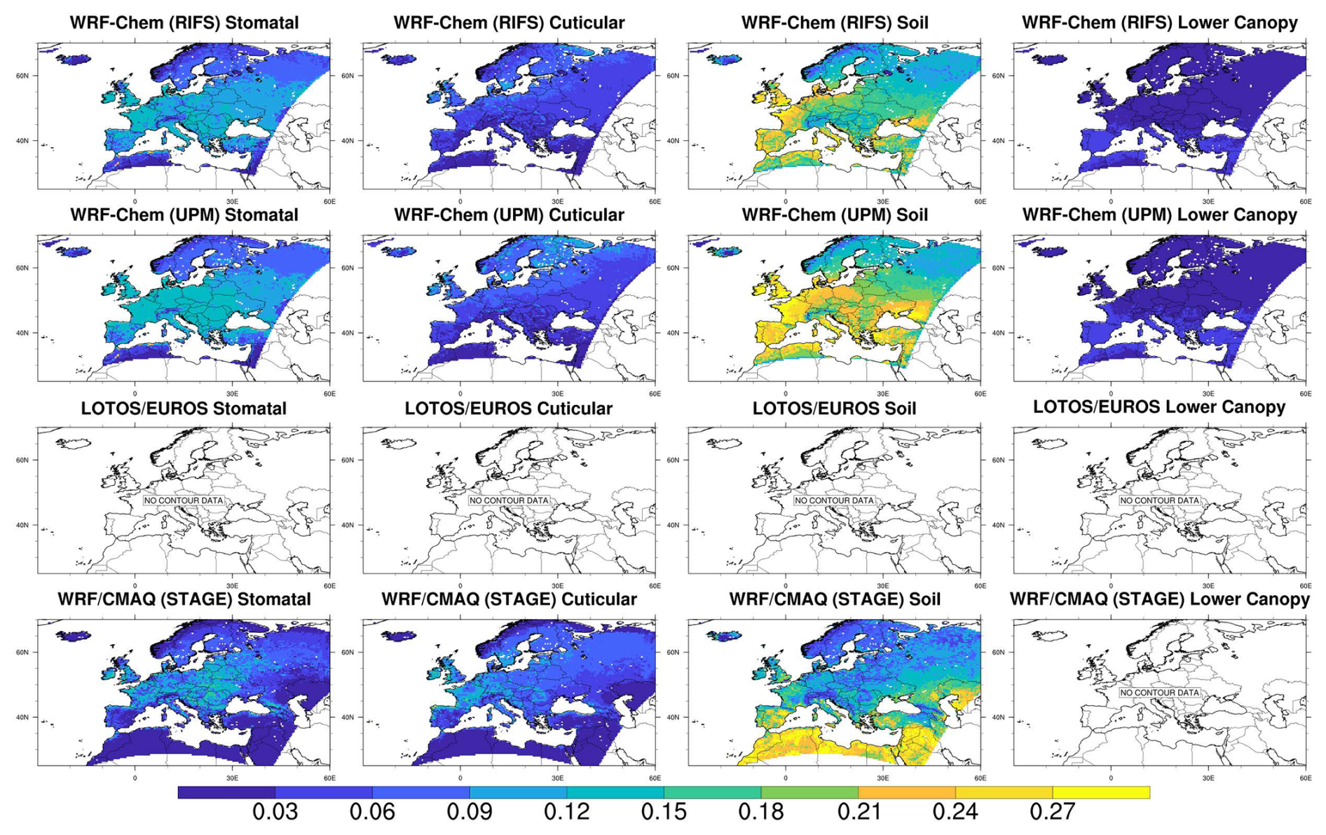
Figure 8 Absolute grid-scale ozone effective conductances (cm s⁻¹), averaged over the entire year. Results are for the NA domain during 2016. Note that these maps are not clipped to the domain common to all simulations and show the maximum spatial extent of non-water cells submitted for each model.

The impact of factors other than the dry deposition scheme itself on simulated V_d and pathway contributions is further illustrated by the comparison of the three WRF-Chem simulations performed over NA and the two WRF-Chem simulations performed over EUR. These simulations all use the WRF-Chem implementation of the Wesely scheme and as a result all share similar relative pathway contributions to V_d, but V_d itself shows a variation of roughly 25 % over NA and 15 % over EUR between these simulations. All three of these models make use of feedbacks between aerosols and meteorology, and hence other parameterization differences in addition to the gas-phase deposition code influence the resulting gas-phase deposition velocities, through changes in the predicted temperature, relative humidity, and the other meteorological terms influencing deposition velocity.

Figures 7–8 depict maps of absolute pathway contributions to annual mean V_d over both domains, where the mean is from the average of the monthly median values. The maps show the lower contributions from the cuticular pathway for WRF-Chem compared to other simulations, especially over the eastern US and central Europe. This is consistent with the domain-average contributions shown in Fig. 5. For the models that include the lower canopy pathway as a separate term from the other pathways (all WRF-Chem simulations and two of the GEM-MACH simulations), its contribution to V_d is less than 0.06 cm s⁻¹ throughout both domains (10 % or less of the domain-wide annual means as shown in Figs. 5–6). Both CMAQ simulations and the GEM-MACH (Zhang) simulation tend to have stronger longitudinal gradients over the NA domain for the soil pathway contribution compared to other simulations. The two GEM-MACH simulations using the Wesely dry deposition scheme (GEM-MACH (Base) and GEM-MACH (Ops)) and the WRF-Chem (RIFS) and WRF-Chem (UPM) simulations have noticeably higher absolute soil pathway contributions in the south-central and southeastern US than the other simulations, indicating that the higher values in the domain-average soil pathway contributions for these four simulations shown in Fig. 3 originate in these regions.

Figures S5–S6 show the relative, rather than absolute, contribution of the four pathways to annual mean V_d over both domains, while corresponding maps for summer and winter over NA are included as Figs. S7–S8. These figures show that the WRF-Chem simulations tend to have a weaker spatial variation than the WRF/CMAQ and GEM-MACH simulations in the split between different pathways over both domains, especially for the relative contribution of the soil pathway. For example, the dominance of the stomatal and cuticular pathways over the soil pathway over the eastern US and of the soil pathway over the stomatal and cuticular pathways in the western US that is simulated by WRF/CMAQ and GEM-MACH is less pronounced in the WRF-Chem simulations. Over the EUR domain, the WRF-Chem simulations show a larger relative contribution of the soil pathway than the WRF/CMAQ simulation throughout much of central Europe. For the NA domain, the relative contributions of the cuticular component are highest for WRF/CMAQ over the northeastern US, followed by GEM-MACH and then WRF-Chem. These features are especially pronounced during summer (Fig. S7). For the EUR domain, the relative contribution of the stomatal component is highest for WRF/CMAQ over eastern central Europe and exceeds that of the WRF-Chem simulations.

3.2 LU-specific results

Model-to-model differences in domain-average grid-aggregated V_d and pathway contributions may result from not only different process representations but also different LU spatial distributions and/or LU-dependent parameter and variable choices. It is important to note that the impacts of LU on dry deposition calculations can be both direct (e.g., the incorporation of LU-dependent LAI in some schemes' stomatal and/or cuticular resistance formulations) and indirect and can also vary across schemes depending on the specific formulations of component resistances (Clifton et al., 2023). An example of indirect impacts of LU is the effect of LU-dependent LAI on the calculation of air temperature in the LSM and its subsequent impact on stomatal resistance even in schemes without direct dependence of stomatal resistance on LAI. Another example is the effect of LU on the calculation of ground temperature and relative humidity in the LSM, which are then used in the formulation of cuticular resistance. Thus, examining LU-specific parameters and variables (e.g., roughness length, LAI) and using them to interpret model-to-model differences in V_d and effective conductances are not straightforward, and untangling such direct and indirect effects across the different modeling systems is beyond the scope of the AQMEII4 grid model intercomparison activity. Instead AQMEII4 collected V_d and effective conductances for 16 standardized LU categories in addition to the grid-aggregated values analyzed above. These LU-specific fields allow us to investigate the total (both direct and indirect) impacts of LU-dependent process representations and LU distributions on modeled deposition by stratifying our analyses by LU. Put differently, in this section we treat LU as a proxy for all LU-dependent processes and parameters, meaning that the dependence of model results on LU in this section should be interpreted as being due to “all land-use-dependent quantities in the deposition algorithms used in AQMEII4 models”.

Table 3 (a) Annual mean grid-scale and LU-specific sum of effective conductances (cm s⁻¹) for individual simulations as well as the range of values across all simulations. For a given column and domain, the maximum values are shown in bold and the minimum values are shown in italics. Blank cells indicate that data for a given model, pathway, and/or LU were not available. The grid-scale results reflect spatial averages over all non-water grid cells in the common analysis domain. The LU-specific results reflect spatial averages over all cells for which that LU fraction exceeded 85 % for a given model (note that the number of such cells can vary across models). The LU categories are abbreviated as URB (urban), BAR (barren), ENF (evergreen needleleaf forest), DBF (deciduous broadleaf forest), MF (mixed forest), SHR (shrubland), AGR (planted/cultivated), and GRA (grassland). (b) As in (a) but for the stomatal effective conductances (cm s⁻¹). (c) As in (a) but for the cuticular effective conductances (cm s⁻¹). (d) As in (a) but for the soil effective conductances (cm s⁻¹). (e) As in (a) but for the lower canopy effective conductances (cm s⁻¹).

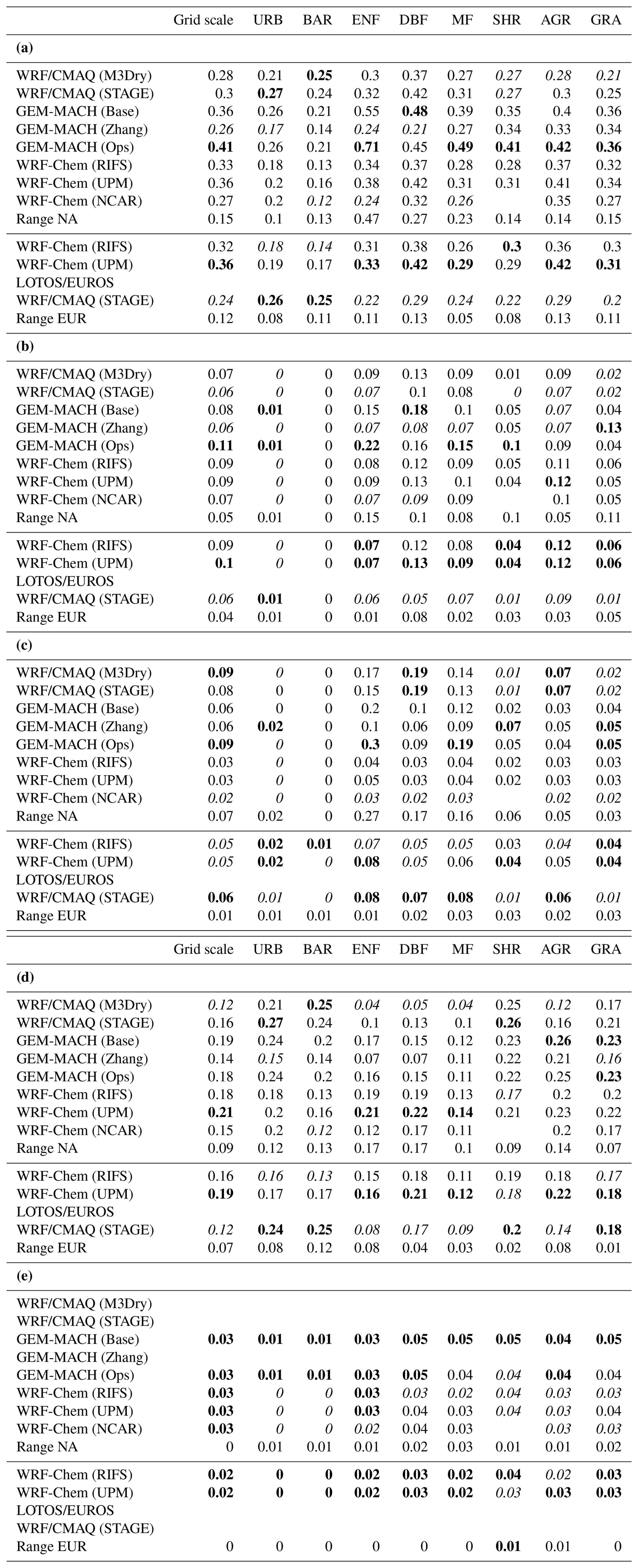
Figure 9 shows the contributions of the four effective conductance pathways to the annual mean V_d for evergreen needleleaf forest for each model over the NA domain, averaged over only those grid cells where a given model had 85 % coverage of evergreen needleleaf forest (note that the number of such grid cells differed across models, as discussed in greater detail in Sect. 3.3). Comparing this figure to the equivalent grid-aggregated results shown in Fig. 5 when all common non-water grid cells were analyzed shows that considering instead only the model grid cells containing a specific LU type can increase model spread. For example, annual mean grid-aggregated V_d ranges from 0.26–0.42 cm s⁻¹ averaged over all common non-water grid cells over NA (Fig. 5), while the range is 0.24–0.71 for V_d for grid cells dominated by the evergreen needleleaf forest category (Fig. 9). Similar increases can also be seen in the ranges of absolute pathway contributions (e.g., soil effective conductance from 0.12–0.21 cm s⁻¹ in Fig. 5 to 0.04–0.2 cm s⁻¹ in Fig. 9) and relative pathway contributions (e.g., cuticular conductance from 7.6 % to 31.7 % in Fig. 5 to 12.6 %–56.4 % in Fig. 9). Results of individual and summed pathway contributions for a total of eight LU categories over both domains are shown in Table 3a–e. These results confirm the general increase in model spread of both V_d and pathway contributions when considering LU-specific diagnostics, especially for V_d and the cuticular and stomatal effective conductances over forested and agricultural LU types. Such increased heterogeneity of process-level diagnostics when considering locations corresponding to specific LU categories compared to locations representing a mix of LU categories is also reported in Kioutsioukis et al. (2025). This finding suggests that LU-dependent parameter choices and the representation of vegetation effects on O₃ dry deposition (e.g., whether or not a given scheme accounts for soil moisture effects on stomatal conductance) are a significant source of variability in grid-aggregated V_d while also indicating that an analysis of only grid-aggregated deposition diagnostics may partially mask the effects of process-specific differences that exist between schemes. However, the attribution of LU-specific diagnostics to LU-dependent parameter choices is complicated by potential model-to-model differences in LU distribution; for example, differences in the number and location of grid cells with a given LU type in a given modeling system may cause differences in macro-scale meteorological variables like wind speed and solar radiation that affect the deposition calculations in this LU-specific analysis. Differences in LU distributions between models are analyzed in Sect. 3.3.

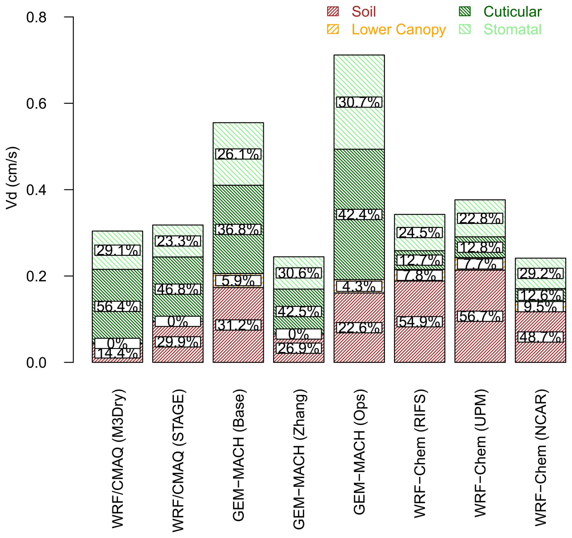
Figure 9 2016 annual domain-average LU-specific effective conductances and ozone deposition velocities for evergreen needleleaf forest over the NA domain. Averages were calculated over all grid cells in the portion of the analysis domain shared by all model simulations for which a given model had coverage of at least 85 % for the evergreen needleleaf forest LU category.

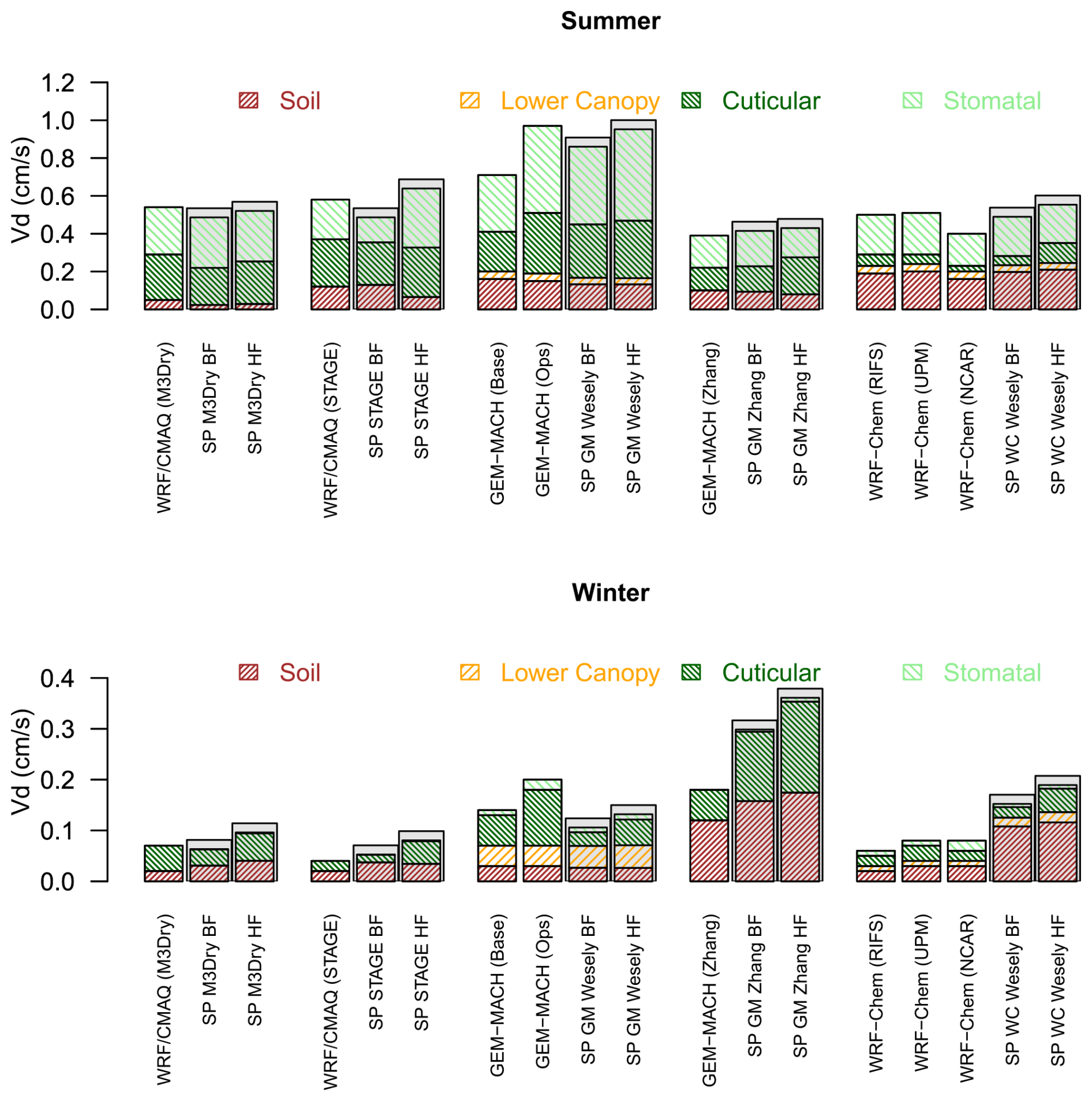
Figure 10 Summer and winter effective conductances and ozone deposition velocities calculated by the grid models for mixed-forest grid cells and calculated by the corresponding subset of single-point (SP) models analyzed in Clifton et al. (2023) at the Borden Forest (BF) and Harvard Forest (HF) sites. The bars for the SP models are overlaid on grey boxes to visually distinguish them from the bars representing grid models. In the x-axis labels, results for the SP GEM-MACH (Wesely) and SP GEM-MACH (Zhang) simulations are shown as “SP GM Wesely” and “SP GM Zhang”, respectively, while results for the SP WRF-Chem (Wesely) simulations are shown as “SP WC Wesely”. The mixed-forest grid cells selected for this analysis are those in which a given model had at least 85 % coverage for this LU category. The number of these grid cells differs across models due to underlying differences in LU (see Sect. 3.3).

The availability of LU-specific dry deposition diagnostics from the AQMEII4 grid models also provides an opportunity to compare these diagnostics to the results from the point model intercomparison study by Clifton et al. (2023). At each of the eight O₃ flux measurement sites examined in Clifton et al. (2023), the point model simulations were constrained to use a common set of site-specific variables like LAI, roughness length, reference height, and soil moisture. Figures 10 and S6–S8 show examples of this comparison. In these figures, bars showing the single-point model results from Clifton et al. (2023) are prefixed with the label “SP” to more easily distinguish them from bars showing the grid model results, and the point model labels also use abbreviations for GEM-MACH and WRF-Chem as noted in the figure caption. Figure 10 compares winter and summer average V_d and effective conductances simulated by the grid models for grid cells with mixed-forest coverage greater than 85 % against the corresponding results for single-point models at the two mixed-forest sites analyzed in Clifton et al. (2023), i.e., Borden Forest and Harvard Forest. The point model results are identical to those shown in Fig. 5 of Clifton et al. (2023), but while 18 point simulations were included in that figure, only the 5 simulations corresponding to the schemes appearing in Clifton et al. (2023) that were also implemented in the AQMEII4 grid models (CMAQ (M3Dry), CMAQ (STAGE), GEM-MACH (Wesely), GEM-MACH (Zhang), and WRF-Chem (Wesely)) are reproduced here. Also note that while the seasonal grid model values shown in Fig. 10 are derived for a single year (2016) but averaged over all grid cells for which a given model had a fractional coverage of mixed forest exceeding 85 %, the point model values at Borden Forest and Harvard Forest are multi-year means at single sites. The motivation for performing this comparison despite these differences in spatio-temporal aggregation is to assess to which extent the conclusions of a single-point modeling study are consistent with results obtained from grid model deposition diagnostics and could therefore inform grid model development by providing process-level insights.

A comparison of the summertime grid model and point model results in Fig. 10 leads to similar conclusions regarding the magnitudes of simulated V_d and pathway contributions across models. For example, both grid model and point model V_d values range between 0.4 and 1.0 cm s⁻¹ across models. The lowest V_d for the point models is simulated by GEM-MACH (Zhang), while the highest V_d is simulated by GEM-MACH (Wesely). This is consistent with the grid model results, with GEM-MACH (Zhang) showing lower V_d than all other grid models and GEM-MACH (Base) and GEM-MACH (Ops) showing higher V_d than all other grid models. Grid and point models also agree that CMAQ (M3Dry) has a much smaller contribution of the soil effective conductance to V_d compared to all other models and that WRF-Chem (Wesely) has a smaller contribution of the cuticular effective conductance to V_d compared to all other models.

During winter, the point and grid model results show consistency in terms of relative model rankings (GEM-MACH (Zhang) and the corresponding grid model simulations GEM-MACH (Base) and GEM-MACH (Ops) have the highest V_d, while the CMAQ (STAGE) point and grid model simulations have the lowest V_d), the magnitude of V_d (ranging from about 0.1 to about 0.35 cm s⁻¹), and model-to-model variations in pathway contributions. However, the grid model results show a generally lower V_d and a different ranking than the point model results, with GEM-MACH (Wesely) V_d roughly equal to GEM-MACH (Zhang) in the point model comparison rather than significantly lower when comparing the corresponding grid model simulations GEM-MACH (Base), GEM-MACH (Ops), and GEM-MACH (Zhang). Spatial variations in snow cover across the mixed-forest grid cells in the grid models as well as interannual variability in snow cover at the flux measurement sites may play a role in causing these wintertime differences, although Clifton et al. (2023) found that the point models results were not very sensitive to snow cover. The results of the grid model and point model analysis agree on the non-negligible wintertime contribution of the lower canopy pathway for the models that consider it, i.e., the GEM-MACH (Wesely) (20 %–40 % across the corresponding grid and point models) and WRF-Chem (Wesely) (10 %–14 % across the corresponding grid and point models) point models and their corresponding grid model implementations.

Figures S9, S10, and S11 show corresponding results for evergreen needleleaf forest, broadleaf deciduous forest, and grassland, respectively. For each of these LU cases, the grid model results reflect simulated LU-specific V_d and effective conductances averaged over all grid cells with coverage greater than 85 % for that LU category for a given model. The point model results adapted from Fig. 5 of Clifton et al. (2023) are for Hyytiälä (evergreen needleleaf forest), Ispra (deciduous broadleaf forest), and Bugacpuszta and Easter Bush (both grassland).¹ The results for evergreen needleleaf and deciduous broadleaf forest in Figs. S9 and S10 are broadly consistent with those discussed above for mixed forest. In particular, agreement between grid and point modeling results is generally better during summer than winter, especially in terms of the GEM-MACH (Wesely) vs. GEM-MACH (Zhang) comparison. The non-negligible contribution of the wintertime lower canopy effective conductance simulated by GEM-MACH (Wesely) and, to a lesser extent, WRF-Chem (Wesely) discussed above for mixed forest is also visible in the deciduous broadleaf forest results, for both grid and point models, while it is less pronounced for evergreen needleleaf forest. The model-to-model comparisons for grassland show consistent behavior between the grid model and point model analyses for both winter and summer. During winter GEM-MACH (Zhang) and WRF-Chem (Wesely) show the highest V_d, while GEM-MACH (Wesely) shows the lowest V_d. During summer, GEM-MACH (Wesely) V_d exceeds GEM-MACH (Zhang) V_d for both the grid model results and both grassland point intercomparison sites, though summertime GEM-MACH (Zhang) V_d for grassland is not as low relative to other models as for the different forest LU categories discussed above. Moreover, both grid model and point model results for summertime also agree that GEM-MACH (Zhang) has the largest relative contribution of the stomatal effective conductance to V_d for grassland.

Table 4 Mapping of LU classes from the categories used in the models' dry deposition code to the 16 AQMEII4 categories.

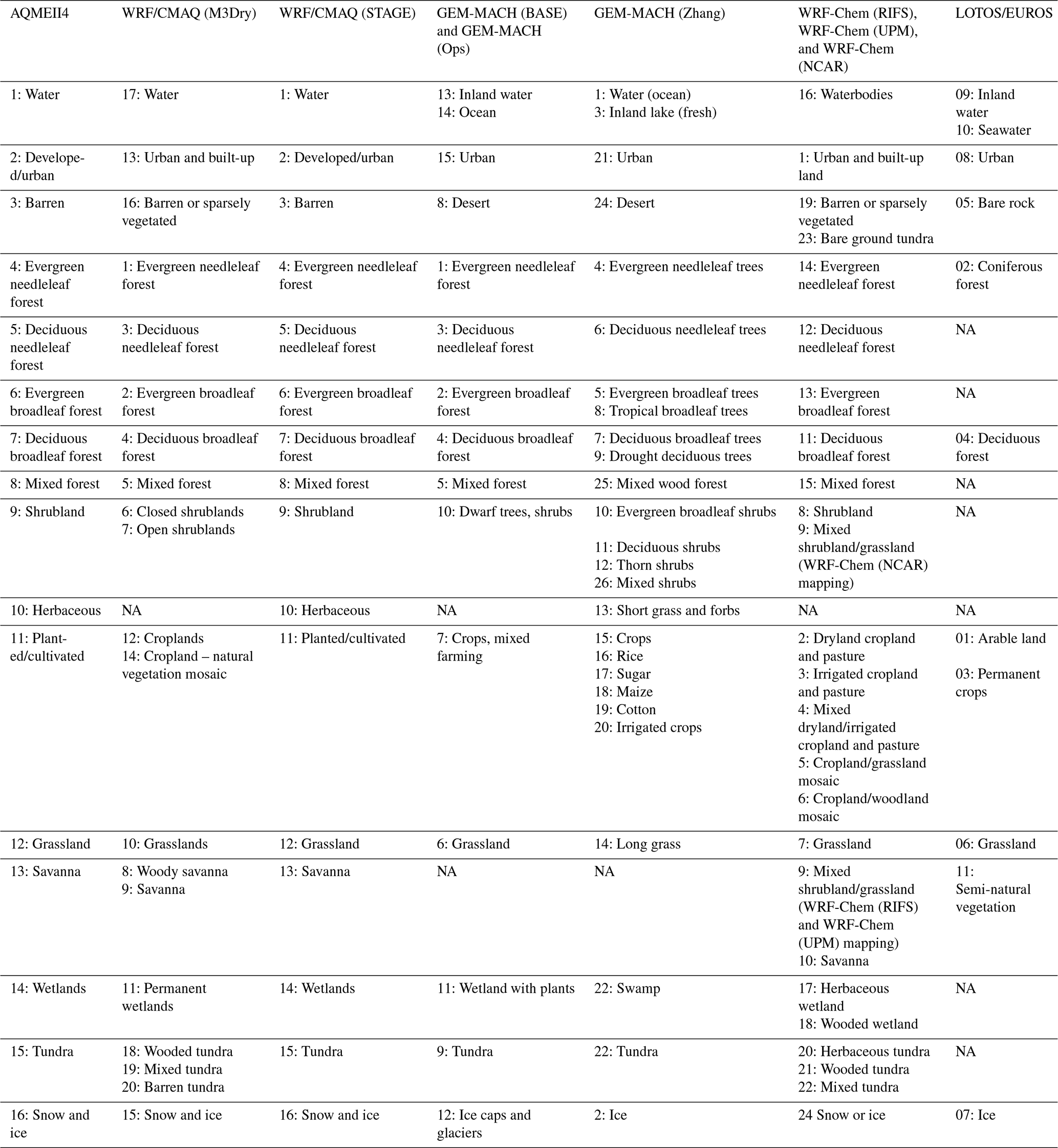
NA: not available.

The results presented above demonstrate that despite differences in LU in the region of the observation sites at the scale of model grid cells, the analysis of O₃ dry deposition schemes implemented in grid models can successfully be linked to the detailed point model evaluation using long-term O₃ flux measurements presented in Clifton et al. (2023) when generating LU-specific diagnostic information and limiting the analysis to specific LU categories. This in turn allows the developers of grid models to leverage process-level insights gained from point intercomparison studies (Clifton et al., 2023; Khan et al., 2025) for improving the representation of dry deposition in their modeling systems. In addition, the general agreement between the grid and point model comparisons shown in Figs. 10 and S7–S9 again suggests that the differences in first-layer heights between the grid models (Table 1) are not a major factor impacting the interpretation of V_d and effective conductance differences across models since reference and displacement heights had been harmonized in the point model calculations. However, as also discussed in the first part of this section, differences in LU characterizations between models can complicate a process-level attribution of differences across models to differences in deposition schemes, especially when considering LU-specific dry deposition fluxes. Similarly, observation sites with a variety of LU within a short distance of the measurement location itself may be less useful for evaluating LU-specific aspects of deposition algorithms. Model differences in LU distributions and their effects on deposition fluxes are analyzed in the next section.

3.3 The influence of land use data on ozone deposition

Table 4 shows the native LU categories used in each model's dry deposition calculations and how these categories were mapped to the 16 common AQMEII4 LU categories defined in Galmarini et al. (2021) when reporting LU-specific diagnostics. For some models (WRF/CMAQ (M3Dry), GEM-MACH (Zhang), WRF-Chem (RIFS), and WRF-Chem (UPM)), the native LU categories used in the dry deposition calculations are identical to those used in the land surface model (LSM) of the driving meteorological model. For the other models, the LU classification scheme differed between the LSM in the driving meteorological model and the dry deposition calculations, and Tables S1–S5 provide details on the internal mapping between the LSM and dry deposition calculations implemented in these models. We note that several AQMEII4 LU categories are held in common with most model native LU categories (e.g., “evergreen needleleaf trees”), while others were less direct, requiring assignment into the nearest AQMEII4 LU category as documented in these tables.

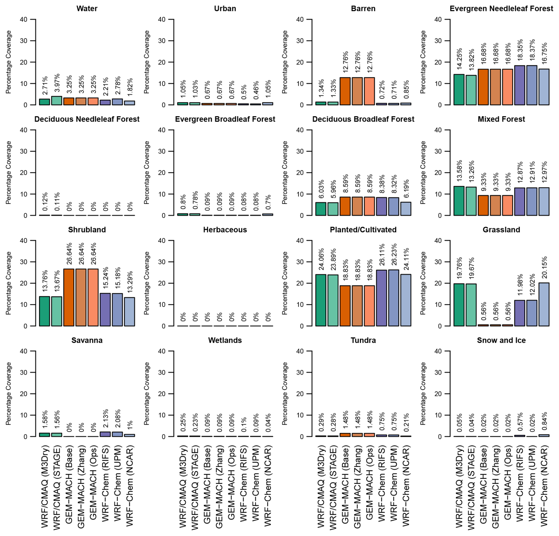
Figure 11 Fraction of the NA domain common to all models covered by each AQMEII4 LU category, excluding grid cells dominated by water by each model.

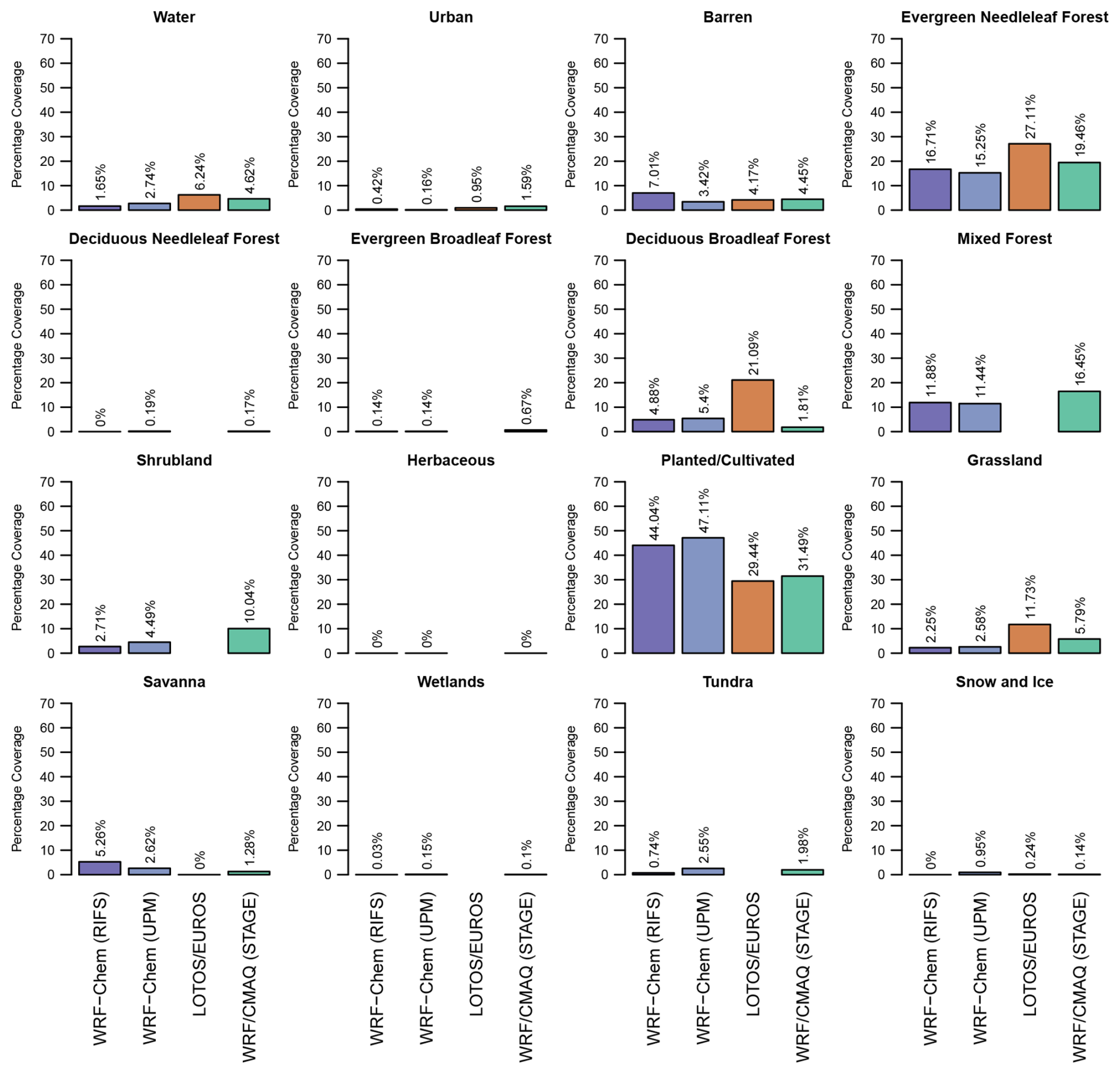
Figure 12 Fraction of the EUR domain common to all models covered by each AQMEII4 LU category, excluding grid cells dominated by water by each model.

Figures 11 and 12 show bar charts of the distribution of all 16 AQMEII4 LU categories for each model across all common grid cells that are not dominated by water for the NA and EUR domains. These charts reveal that 7 of the 16 categories (barren, evergreen needleleaf forest, deciduous broadleaf forest, mixed forest, shrubland, planted/cultivated land, and grassland) account for roughly 90 % of all LU over both NA and EUR. Over NA, the fractional coverage of some categories like evergreen needleleaf forest is similar across models, as might be expected from the commonality of this LU within the native LU categories of Table 4. On the other hand, there is considerable disagreement between models for the fractional coverage of many other categories over NA, especially non-forest categories such as barren, shrubland, planted/cultivated land, and grassland. Much of this disagreement is caused by the GEM-MACH simulations having larger fractions of the barren and shrubland categories and smaller fractions for the planted/cultivated and grassland categories than either the WRF/CMAQ or WRF-Chem simulations, pointing to ambiguities in classifying non-forest partially vegetated areas.² Over EUR, the primary driver of model variability in the LU used for deposition calculation is LOTOS/EUROS, which in its DEPAC dry deposition module splits mixed forest from the driving meteorological model equally between coniferous and deciduous forest and includes shrubland in the category of semi-natural vegetation and as a result shows larger coverage than WRF/CMAQ and WRF-Chem for evergreen needleleaf forest, deciduous broadleaf forest, and grassland. In addition, while all models agree that planted/cultivated is the dominant category over EUR, the lowest coverage (29.44 %, LOTOS/EUROS) and highest coverages (47.11 %, WRF-Chem (UPM)) differ by a factor of 1.6. Here it should be noted that the WRF-Chem (RIFS) dry deposition calculations indirectly used the CORINE dataset developed for Europe (https://land.copernicus.eu/pan-european/corine-land-cover/, last access: 12 May 2025) by mapping the CORINE categories to the USGS24 categories in WRF-Chem (RIFS). On the other hand, the WRF-Chem (UPM) dry deposition calculations relied on the global USGS24 dataset, WRF/CMAQ relied on the global MODIS dataset augmented by additional urban categories in the greater London area and mapped these to the AQMEII4 categories as shown in Table S1, and the LOTOS/EUROS dry deposition calculations relied on the Global Land Cover 2000 dataset (https://forobs.jrc.ec.europa.eu/glc2000, last access: 12 May 2025) mapped to the internal DEPAC categories (Manders-Groot and LOTOS-EUROS team, 2023).

Even for categories for which models show relatively close agreement of the total domain-wide coverage in Figs. 11 and 12, spatial patterns of the coverage may still differ between models. To illustrate this, Figs. S12 and S13 show maps of the fractional coverage of the evergreen needleleaf forest category for each model over NA and EUR. One fundamental difference between the WRF-Chem simulations and all other simulations is that the WRF-Chem simulations employed a dominant LU category approach in their LSM and dry deposition calculations (that is, only the LU with the largest LU fraction within a grid cell is used to represent that grid cell's LU for deposition calculations), while all other simulations accounted for subgrid variations in LU by employing a fractional LU category approach. Therefore, Figs. S12 and S13 show evergreen needleleaf forest fractions of either 0 or 1 for the WRF-Chem simulations and fractions between 0 and 1 for all other simulations. Both figures reveal that, despite all native LU databases including evergreen needleleaf forest as an explicit LU category, the coverage for this LU can vary substantially between models, e.g., over the southeastern US in the NA domain (Fig. S12) and central Europe and the Iberian Peninsula in the EUR domain (Fig. S13).

Table 5 Number and percentage of grid cells within the common NA and EUR analysis domains where all models agree on the land use–land cover (LULC) category for that grid cell. Two metrics are used to assess agreement: (1) all models agree that the LULC category being assessed is the category with the highest fractional coverage compared to all other categories in that grid cell (“dominant coverage”), and (2) in addition to meeting metric 1, all models also agree that a given grid cell has at least 85 % coverage for the LULC category being assessed. The last four rows summarize the level of agreement across either all 16 LULC categories (including water) or all 15 non-water LULC categories. The percentages shown in the rows corresponding to individual LULC categories are calculated with respect to all grid cells in the common analysis domains (108 058 for NA and 176 994 for EUR).

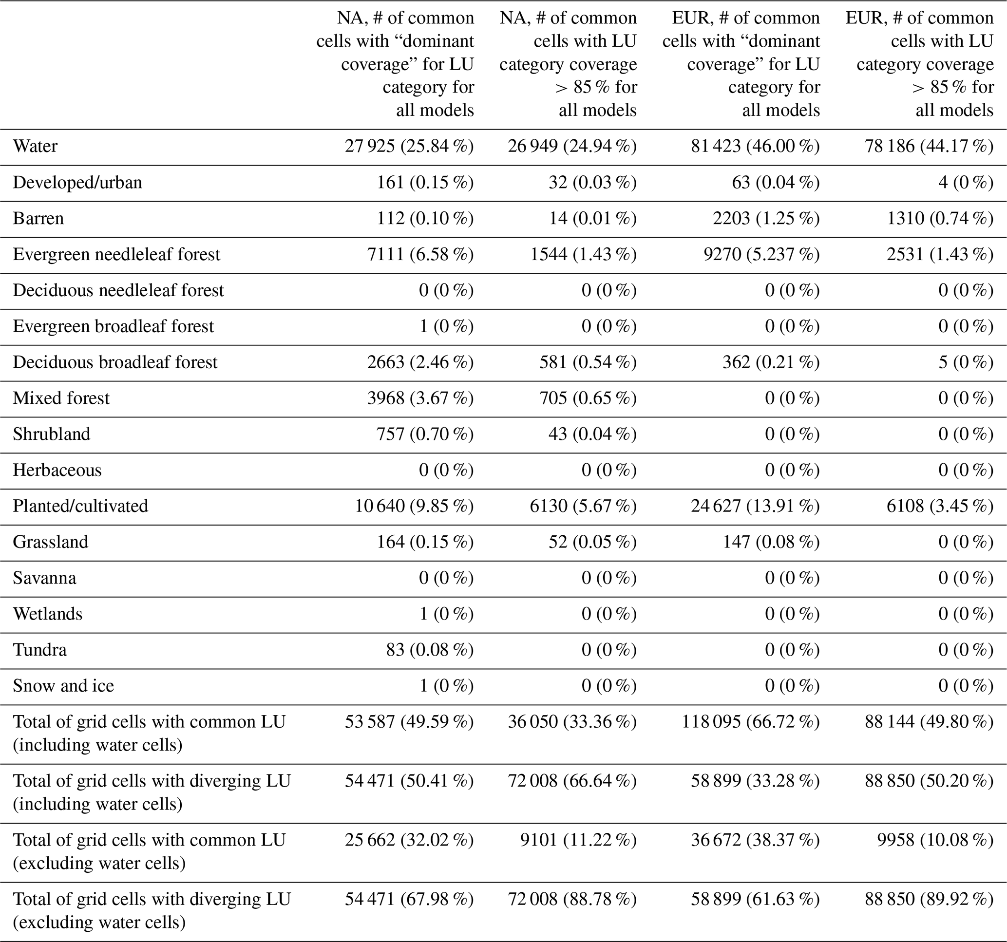
To analyze the level of agreement in spatial coverage across models for all LU categories while taking into account that the WRF-Chem simulations used a dominant LU category approach, we applied two metrics to assess model-to-model agreement for a given LU category and grid cell. The first metric simply determines whether all models agree that the LU category being assessed is the category with the highest fractional coverage (i.e., the dominant category) compared to all other categories in that grid cell, regardless of the actual fractional coverage for that dominant category for those simulations that use a fractional coverage approach. The second metric builds upon the first metric by determining not only whether the LU category being assessed is the dominant category in that grid cell but also whether all models agree that its fractional coverage is at least 85 %. By definition, all grid cells meeting the more stringent second metric also meet the first metric. Identifying grid cells meeting the first metric can be thought of as a way to assess agreement in LU categories across models if all simulations (not only WRF-Chem) had used a dominant LU category approach. The subset of grid cells identified by metric 1 for a given LU category that also satisfies the > 85 % criterion defined for metric 2 can be thought of as the common “dominant” cells for that LU category in which even the computations performed by the models using a fractional LU category approach were mostly impacted by the physical characteristics of that LU category, with only minor impacts from other LU categories possibly also present in the grid cell.

The results of applying metrics 1 and 2 to all LU categories and models over both NA and EUR are shown in Figs. S14–S15 and Table 5, which lists the number and percentage of grid cells within the common NA and EUR analysis meeting each metric. The first 16 rows of Table 5 contain results for each of the AQMEII4 LU categories. The percentages shown in these rows are calculated with respect to the total number of grid cells in the common analysis domains (108 058 for NA and 176 994 for EUR), including water grid cells. Water is by far the category with the highest level of agreement over both NA and EUR, with only minor differences between the two metrics, indicating that most grid cells dominated by water across all models are almost fully (>85 %) or often fully covered by water, reflecting the oceans and open waters present in both analysis domains.

The LU categories with the second- and third-largest amount of agreement between models are planted/cultivated land and evergreen needleleaf forest over both domains. Over NA, the deciduous broadleaf and mixed-forest LU categories also have about 600–4000 (0.5 %–4 %) common grid cells, depending on metric and category. For the remaining LU categories, the number and percentage of grid cells matching across models is very low, especially for the more stringent metric 2. While to some extent this is expected given the low overall domain coverage of some of these categories by all models (Figs. 11–12), this is also the case for shrubland and grassland, which have substantial domain-wide coverage over NA (Fig. 11).

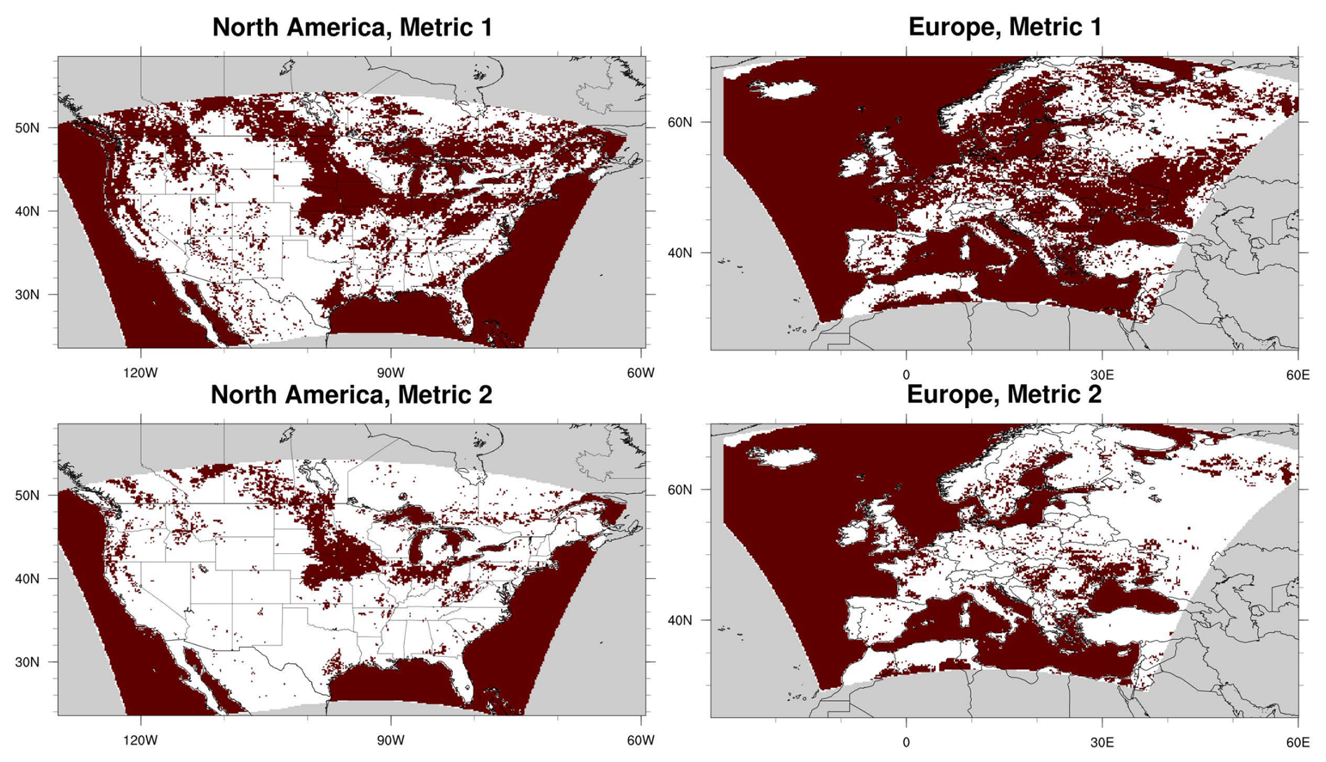
Figure 13 Red areas indicate grid cells meeting metrics 1 and 2 used to assess LU communality across models as described in the text.

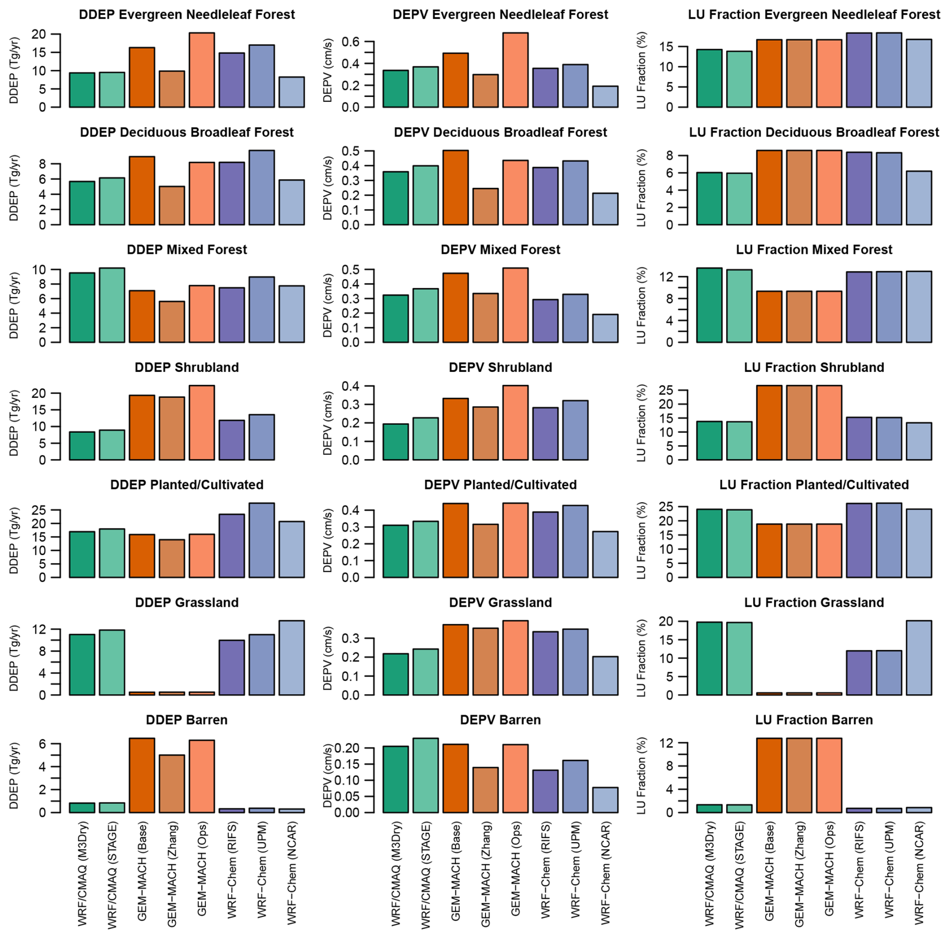
Figure 14 LU-specific annual domain-total dry deposition (DDEP) fluxes (Tg), LU-specific annual mean dry deposition velocity (DEPV; cm s⁻¹), and percentage of LU category domain coverage (excluding water grid cells) for seven selected LU categories over the NA domain. For each LU category and model, the analysis considered grid cells in the analysis domain common to all models in which a given model had at least 85 % coverage for this LU category. The number of these grid cells differs across models due to underlying differences in LU (see Sect. 3.3).

The last four rows of Table 5 summarize the level of agreement across either all 16 LU categories (including water) or the 15 non-water LU categories. Figures 13a–d depict the location of common grid cells for both metrics and continents. In these figures, grid cells meeting the metric for any LU category are colored in dark red, while grid cells not meeting it for any LU category (i.e., grid cells without a common LU category as measured by the metric) are colored in white. These figures along with Table 5 illustrate that even for the less restrictive metric 1, 68 % (62 %) of non-water grid cells over NA (EUR) do not share a common dominant LU category across models. Over NA, many of these non-matching grid cells are located in the southern and western portions of the domain, while over EUR, they are most prevalent in the western, northeastern, and southeastern portions of the domain. When considering the more stringent metric 2, i.e., grid cells in which the common category has at least 85 % coverage for all models, this number of grid cells with diverging LU categories increases to roughly 90 % of non-water grid cells over both domains. The only areas with significant contiguous clusters of such common cells are the agricultural regions in the north-central NA domain and portions of central Europe and Sweden.

This low number of grid cells with a common LU category strongly suggests that differences in LU coverage can contribute to or even drive differences in LU-specific dry deposition fluxes, in addition to any differences in process representation that exist between different models. To investigate this, Fig. 14 compares LU-specific dry deposition fluxes, V_d, and LU fractions over NA for seven selected LU categories. The LU-specific dry deposition fluxes (V_d) represent annual totals (means) over all grid cells in which the LU category being assessed has a fractional coverage of at least 85 % for a given model. For some LU categories with relatively similar total coverage across the domain (e.g., evergreen needleleaf forest and deciduous broadleaf forest), differences in total O₃ dry deposition flux to that LU category closely mirror differences in LU-specific average V_d. For mixed forest, the lower fractional coverage for GEM-MACH (Base) and GEM-MACH (Ops) leads to a below-average total deposition flux to that category despite V_d being the highest. For the grassland and barren categories, differences in their dry deposition fluxes are almost entirely driven by differences in LU fractional coverage rather than differences in V_d. Corresponding results for the EUR domain are shown in Fig. S16 and confirm that differences in both V_d and LU coverage contribute to differences in LU-specific dry deposition fluxes.

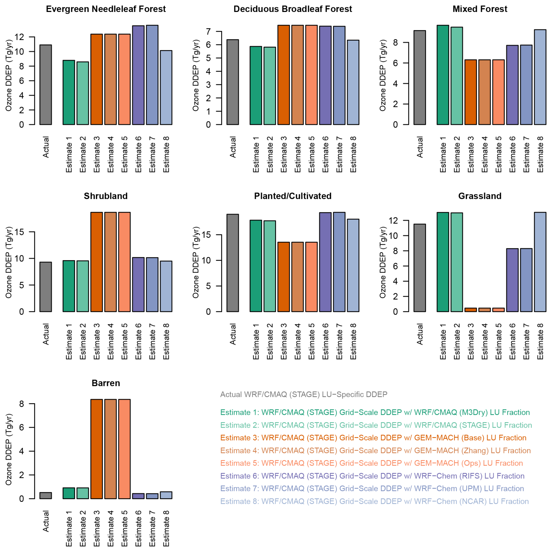
Figure 15 2016 NA annual domain-wide total ozone dry deposition fluxes (Tg yr⁻¹) for selected LU categories. The grey bar shows LU-specific fluxes calculated by WRF/CMAQ (STAGE), while the colored bars show LU-specific fluxes estimated by combining WRF/CMAQ (STAGE) grid-scale fluxes with LU fractions from other models as described in the text.

The results shown in Figs. 14 and S14 have important implications for computing estimates of deposition fluxes to specific ecosystems. In past model intercomparison studies such as those performed under the umbrella of the Task Force on Hemispheric Transport of Air Pollution (TF-HTAP; http://www.htap.org, last access: 19 August 2025), such estimates were often computed through post-processing by apportioning archived modeled grid-aggregated dry deposition fluxes to specific LU categories using a fixed LU database (e.g., Hardacre et al., 2015; Schwede et al., 2018). While this approach makes use of actual modeled dry deposition fluxes rather than using modeled concentrations as inputs to offline dry deposition calculations (e.g., Van Dingenen et al., 2009; Avnery et al., 2011), it may still be subject to uncertainties arising from differences between grid-aggregated vs. LU-specific dry deposition fluxes as well as differences in LU categorization – a flux associated with a model LU category for model-internal deposition may be aggregated under a different LU category in post-processing using a different post-processing database. The diagnostic information collected for AQMEII4 and analyzed in this paper allows us to illustrate and quantify both uncertainties. Figure 15 compares the LU-specific annual total dry deposition fluxes to seven LU categories calculated by model WRF/CMAQ (STAGE) (grey bars) to estimates derived by combining grid-aggregated dry deposition fluxes from the same model with LU fractions from all models (colored bars). Comparing the grey bars to the dark-blue bars shows the impact of computing actual LU-specific deposition fluxes within the model simulation vs. estimating them by linearly scaling grid-aggregated values using the model's own LU fractions. This effect is relatively small for most LU categories but reaches about 20 % for evergreen needleleaf forest and 40 % for barren. Comparing the grey bars to all the other colored bars (except dark blue) shows the combined uncertainty of using linear scaling of grid-aggregated deposition values and using different LU datasets than the one used within the model to calculate the LU-specific value. These differences are generally much larger and reflect the substantial divergence in LU categories across models, due to the variety of native model LU databases in use between different models. This example demonstrates the advantage of computing and collecting LU-specific diagnostic dry deposition information in model intercomparison studies so that model-to-model differences in deposition estimates can be tied to differences in model-specific process representation and LU datasets. Potential future work to harmonize LU datasets across models would allow for further constraining differences to process representations only. This in turn would make it easier to leverage insights gained from point intercomparison studies (Wu et al., 2018; Clifton et al., 2023; Khan et al., 2025) for improving the representation of dry deposition in grid models.

4 Summary

This study presented a diagnostic analysis of ozone dry deposition from annual AQMEII4 photochemical grid modeling simulations performed over NA and EUR. Simulated annual O₃ dry deposition fluxes ranged from 59.5 to 91.4 Tg yr⁻¹ over the NA domain and from 47.2 to 82.9 Tg yr⁻¹ over the EUR domain. Analysis of grid-aggregated effective conductances showed that models with a similar V_d can exhibit significant differences in the absolute and relative contributions of different pathways to V_d. The availability of effective conductances also allowed for an attribution of model differences in V_d to specific processes. For example, GEM-MACH (Base), GEM-MACH (Ops), and WRF-Chem (RIFS) all have similar soil and lower canopy effective conductances, revealing that the differences in V_d between these simulations stem from differences in the cuticular and, to a lesser extent, stomatal pathways.

Analysis of LU-specific V_d and effective conductances revealed a general increase in model spread compared to analyzing grid-aggregated values, especially for V_d and the cuticular and stomatal effective conductances over forested and agricultural LU types. This finding suggests that LU-dependent parameter choices and the representation of vegetation effects on O₃ dry deposition are a significant source of variability in grid-aggregated V_d while also indicating that an analysis of only grid-aggregated deposition diagnostics can mask process-specific differences that exist between schemes. Utilizing the LU-specific diagnostics available from the grid model simulations also provided an opportunity to compare these diagnostics to the results from the single-point model intercomparison study by Clifton et al. (2023). Results showed good agreement between the behavior of different dry deposition schemes in single-point models at individual sites vs. their implementation in grid models in aggregate across either the NA or EUR domain for a given LU type. For example, both grid model and point model V_d ranged between 0.4 and 1.0 cm s⁻¹ across models for mixed-forest grid model results and the corresponding point model results at Borden Forest and Harvard Forest, with the lowest V_d associated with GEM-MACH (Zhang) and the highest V_d associated with GEM-MACH (Wesely) in both comparisons. Grid and point models also agreed that WRF/CMAQ (M3Dry) had a much smaller contribution of the soil effective conductance to V_d compared to all other models and that WRF-Chem (Wesely) had a smaller contribution of the cuticular effective conductance to V_d compared to all other models. This demonstrates that the analysis of O₃ dry deposition schemes implemented in grid models can successfully be connected to detailed point model evaluation studies using long-term O₃ flux measurements when generating LU-specific diagnostic information and limiting the analysis to specific LU categories. This in turn allows the developers of grid models to leverage process-level insights gained from point intercomparison studies for improving the representation of dry deposition in their modeling systems. The importance of observation sites being representative of a single LU classification for this purpose has also been noted in this work.

This study also presented a detailed analysis of different models' LU distributions that revealed substantial differences in the spatial patterns and sometimes also the domain-wide coverage of certain LU categories over both domains, especially non-forest partially vegetated categories such as agricultural areas, shrubland, and grassland. Overall, 68 % (62 %) of non-water grid cells over NA (EUR) were found not to share a common dominant LU category across models. When considering only grid cells in which the common dominant category has at least 85 % coverage for all models, this number of grid cells with diverging LU categories increased to roughly 90 % of non-water grid cells over both domains. By comparing LU distributions, LU-specific V_d, and LU-specific dry deposition fluxes, we demonstrate that differences in LU coverage can contribute to or even drive differences in LU-specific dry deposition fluxes, in addition to any differences in process representation that exist between different models. For mixed forest, the lower fractional coverage for GEM-MACH (Base) and GEM-MACH (Ops) leads to a below-average total deposition flux to that category despite V_d being the highest. Differences in the grassland and barren dry deposition fluxes over the NA domain are almost entirely driven by differences in LU fractional coverage rather than differences in V_d. On the other hand, for LU categories that have similar total domain-wide coverage across models (e.g., evergreen needleleaf forest and deciduous broadleaf forest), differences in total O₃ dry deposition fluxes to that LU category closely mirror differences in LU-specific average V_d, indicating that in this case differences in process representation drive differences in fluxes.

Finally, we contrasted the LU-specific dry deposition fluxes simulated in AQMEII4 to estimates in which grid-aggregated fluxes were linearly apportioned to specific LU categories based on LU fractions. When using a consistent set of LU information between the direct simulation of LU-specific fluxes and the apportionment of grid-aggregated fluxes to LU categories based on LU fractions, differences in domain-wide LU-specific deposition estimated by both approaches were generally within 10 % but could be as high as 40 % for a given LU category. These variations are caused by the non-linear effects of subgrid LU variability on V_d and deposition fluxes. When allowing for differences in LU distributions between those used in the grid model simulations generating the LU-specific results and those used to apportion grid-aggregated results to specific LU categories, domain-wide LU-specific deposition estimates differed by 50 % or more for a number of categories. This illustrates that inconsistencies in LU representation between the model simulations and the post-processing apportionment approach can introduce substantial uncertainties in estimates of fluxes to specific ecosystems.

Overall, the results in this study demonstrate that the generation of grid-aggregated and LU-specific diagnostic outputs in model application and intercomparison studies can provide valuable information from (i) a model development point of view to better understand drivers of model variability and identify priorities for model improvement and (ii) an impact analysis point of view to distinguish between stomatal vs. non-stomatal deposition and quantify deposition to specific LU types. However, it should also be acknowledged that designing, implementing, collecting, and analyzing these diagnostics in AQMEII4 was resource-intensive, required a high level of coordination across research groups, and resulted in several iterations before the analyses presented in this and other AQMEII4 paper could be completed. Finally, the results of the LU analysis highlight the importance of documenting and analyzing the representation of LU across models. We recommend that future work be aimed at harmonizing this aspect when using CTMs for deposition analyses, in addition to the current standard practice of harmonizing emissions and boundary conditions in intercomparison studies. In addition, such future harmonization efforts should utilize current-generation publicly available high-resolution LU datasets to improve upon some of the currently used datasets that date back more than a decade and would also benefit from close collaboration with the LSM community.