Amazon rainforest ecosystem exchange of CO₂ and H₂O through turbulent understory ejections

We investigate the role of short-term variability in the mean ecosystem exchange of carbon dioxide and water vapour. Specifically, we focus on quantifying how the intermittent turbulent exchange at the forest–atmosphere interface – characterised by sweeps, ejections, and outward/inward interactions – contributes to the mean exchange. To this end, we analyse observations of high-resolution (isotopic) flux measurements taken at 25 m above the forest canopy at the Amazon Tall Tower Observatory (ATTO) during the dry season. We identify short-term turbulent eddies that eject carbon dioxide and water vapour from the understory (0–15 m) into the atmosphere. The H₂O ejected from the understory is shown to be depleted in deuterium (²H) by 10 ‰ compared to H₂O originating from the top canopy. We show that this matches the depleted water isotopic compositions found in understory leaf and soil samples. The diurnal cycle of the net ecosystem exchange (NEE) of CO₂ is presented as a function of the sweeping and ejection motions and understory flux contributions. Understory contributions average 1.4 % of NEE, but they can reach up to 20 %. In exploring the connection between intermittent canopy turbulence and cloud passages, we found a weak relationship (r=0.027) between cloud passages and ejections, without a predominant influence of large clouds. These findings deepen our understanding of the gas exchange of the Amazon rainforest, which may ultimately allow decision-makers to incorporate policies that can prevent the region's transition from a carbon sink to a source.

1 Introduction

Future climate is highly dependent on the response of the biosphere to the enhanced greenhouse effect. Both anthropogenic (e.g. deforestation) and climate feedback (e.g. drought) processes affect the capacity of the rainforest to take up carbon and recycle water across the South American continent (Rosan et al., 2024; Gatti et al., 2021). Direct measurements of the gas exchange can advance our understanding of the underlying processes and allow us to monitor the behaviour of an ecosystem (Baldocchi, 2020).

It is difficult to capture the details of diurnal biosphere–atmosphere exchange using simplified mathematical representations due to highly non-linear exchange processes. One important example is the generally stably stratified layer of air below the canopy crown, which is referred to as the understory (Pedruzo-Bagazgoitia et al., 2023; Machado et al., 2024). This layer has received little scientific attention, as it is disconnected from the regular bulk turbulent exchange of CO₂ and H₂O at the canopy crown that is normally facilitated by unstable atmospheric conditions during daytime. Combining insights from the literature, we hypothesise the following mechanism by which the understory intermittently contributes to the net flux:

1. During characteristic convective days with developing cumulus clouds in the Amazon, a stable decoupled layer is formed under the canopy crown, where local emissions of CO₂, H₂O, and likely also volatile organic compounds (VOCs) are trapped (Pedruzo-Bagazgoitia et al., 2023; Patton et al., 2016; Dupont et al., 2024; Fitzjarrald et al., 1988; Bannister et al., 2023; Thomas et al., 2008).

2. Increased vertical wind speeds (e.g. induced by shear or cloud dynamics) or shading by clouds breaks the stable inversion (Pedruzo-Bagazgoitia et al., 2023; Vilà-Guerau de Arellano et al., 2019, 2024; Lohou and Patton, 2014; Sikma et al., 2018).

3. As a result, air masses with understory characteristics are intermittently ejected up into the atmospheric boundary layer (ABL) (Dupont et al., 2024; Patton et al., 2016).

Here, we investigate how to identify understory ejections in above-canopy, high-frequency observations; what triggers these ejections; and whether the underlying CO₂ and H₂O exchange processes below the canopy can be identified and quantified through measurements above the canopy. Conceptually, we follow the established framework of Shaw et al. (1983), who combined fast fluctuations in the horizontal and vertical velocities u and w to define the most energetic upward motions out of the canopy as “ejections” and downward motions into the canopy as “sweeps”. We applied that framework to fluctuations in the chemical tracers H₂O and CO₂ (Thomas et al., 2008). This allows us to identify and quantify, for the first time, the contribution of the understory ejections to the total net ecosystem exchange (NEE) flux. Then, we investigate pathways that may trigger the understory ejections, in particular the relationship between turbulent ejections and clouds.

2 Methods

We analysed a comprehensive set of measurements obtained during a 2-week intensive campaign (CloudRoots-Amazon22) at the Amazon Tall Tower Observatory (ATTO) in the Central Amazon rainforest in Brazil. Measurements encompassed the leaf scale, the canopy scale, and the ecosystem scale. Initial work from González-Armas et al. (2025) covers the link between the leaf and canopy scales. This paper is instead focused on the ecosystem scale and how it links to known canopy-scale processes. As the canopy-level profiles presented in González-Armas et al. (2025) represent a local sample from a heterogeneous understory, they were not directly linked to the ecosystem scale.

Our measurement set-up was installed on a balcony at 54 $\mathrm{m}\mathrm{a}.\mathrm{g}.\mathrm{l}.$ (above ground level; ≈ 30 m tall canopy). Central to the set-up were an IRGASON EC100 (Campbell Scientific, Logan, USA) and a LI-COR 7500 (from LI-COR Inc, Lincoln, USA), installed at 57 m height. These instruments continuously collected 20 Hz wind fields and concentrations of CO₂ and H₂O. The data were evaluated using the processed and raw output from EddyPro version 7.06 (Fratini and Mauder, 2014) (from LI-COR Inc, Lincoln, USA). Data treatment included double rotation of the wind field and Webb–Pearman–Leuning (WPL) corrections (Wilczak et al., 2001; Webb et al., 1980). An interquartile range (IQR) outlier filter was applied: 2× the IQR was used to clean the isotopic compositions measured with the laser spectrometers (described below), whereas 3.5× the IQR was employed for the mole fraction and wind field data (similar to Moonen et al., 2023). The time series of the isotope analysers and the eddy-covariance (EC) system were aligned using the H₂O or CO₂ mole fraction signals measured by both (Moonen et al., 2023). Here, the 20 Hz wind and mole fraction data from the EC were subsampled to match the 4 or 10 Hz frequencies of the isotope sensors.

In addition to this backbone of high-frequency wind and atmospheric composition data, two high-flow-rate laser spectrometers measured isotopic compositions of H₂O (Picarro L2130-I) and CO₂ (Aerodyne TILDAS-CS) (Moonen et al., 2023). The analysers were placed on the 54 m balcony in temperature-controlled enclosures, which were set to 35°C to be consistently warmer then the environment (T_max 32°C). Air was drawn to the analysers via an 8 m, $\mathrm{1}/\mathrm{2}$ in. (12.7 mm), heated copper inlet line positioned at 30 cm from the centre of the anemometer tubing at high flow rates (>20 L min⁻¹) to ensure turbulent conditions. An aluminium mesh inlet filter was used as an improvement to our previous field deployment (Moonen et al., 2023). Isotopic compositions are reported as δ values vs. the international reference material Vienna Standard Mean Ocean Water (VSMOW; Mook and Geyh, 2000). The calibration procedures are described in Appendix A2.

2.1 Quadrant analysis

Quadrant analysis provides a way to visualise and quantify variability within a 30 min flux interval by studying the short time deviations in wind and scalars from which the flux was calculated. The variations in vertical and horizontal wind (u,w) or the heat flux (w,T) are often investigated (Thomas and Foken, 2007). We instead looked at a quadrant analysis of CO₂ and H₂O to best differentiate respiration and photosynthesis signals (Thomas et al., 2008) co-located with the wind perturbation signals. While similar features can be found in both the u–w and CO₂–H₂O quadrants, Q₁ in u–w space is not necessarily related to Q₁ in CO₂–H₂O space (Fig. A5).

From this quadrant analysis of H₂O and CO₂, quadrant-specific fluxes $F_{Q_i}$ were derived for each 30 min interval. Each quadrant flux can be linked to an exchange mode, possibly related to a specific process and contributing to the total flux F_tot. Each resulting quadrant flux was multiplied by the fraction of data points present in the respective quadrant ($\frac{n_{Q_i}}{n_{\text{tot}}}$). The addition of the four partial fluxes equals the original 30 min flux (see Figs. 2 and A7).

$$\begin{array}{}\text{(1)}& {\displaystyle }{\displaystyle }{F}_{\text{tot}}=\sum _{i=\mathrm{1}}^{\mathrm{4}}{F}_{Q_i}={\mathit{\rho }}_{\mathrm{m}}\sum _{i=\mathrm{1}}^{\mathrm{4}}\stackrel{\mathrm{‾}}{w_{Q_i}^{\prime }{\mathit{\chi }}_{Q_i}^{\prime }}{\displaystyle \frac{n_{Q_i}}{n_{\text{tot}}}}\end{array}$$

Here, ρ_m is the molar density of air (in mol m⁻³) and χ^′ is a time series of mole fraction fluctuations after Reynolds decomposition. Note that the fluctuations from the mean are based on the data from all four quadrants.

Thomas et al. (2008) also used the CO₂–H₂O quadrant visualisation and identified data in Q₁ as the respiration contributions to the flux. They used a hyperbolic cutoff to isolate the ejection signals from the normalised detrended CO₂ and H₂O time series, which operates as follows:

$$\begin{array}{}\text{(2)}& {\displaystyle }{\displaystyle }lim<{\displaystyle \frac{x^{\prime }}{\mathit{\sigma }\left(x^{\prime }\right)}}\cdot {\displaystyle \frac{y^{\prime }}{\mathit{\sigma }\left(y^{\prime }\right)}}.\end{array}$$

Here, lim indicates the value of the cutoff, and x^′ and y^′ represent the time series of the variable of interest. We found that a hyperbolic cutoff resulted in many data points from the bulk exchange mode being falsely identified as ejections (Fig. 1). In contrast, the hyperbolic cutoff did work well for detecting wind sweeps and ejections in u^′–w^′ space (Fig. A5).

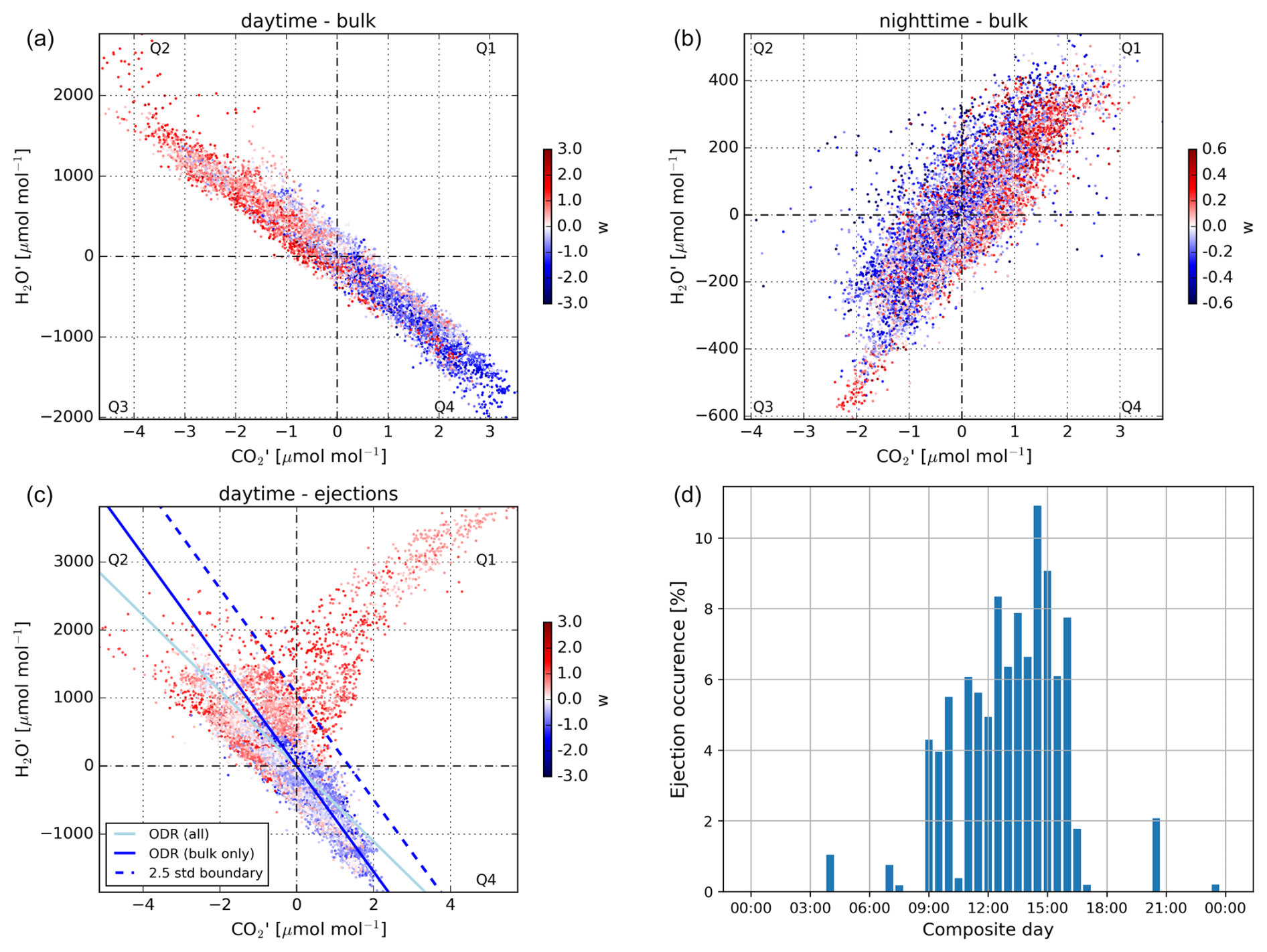
Figure 1 Panels (a), (b), and (c) display 30 min anomalies in the H₂O and CO₂ mole fraction. Individual points are anomalies in the raw 10 Hz data relative to the 30 min mean. The interval in panel (a) runs from 14:00 to 14:30 LT on the 19 August and represents the typical daytime bulk exchange. The interval in panel (b) runs from 23:30 to 24:00 LT on the 20 August and represents the typical night-time bulk exchange. The interval in panel (c) runs from 12:15 to 12:45 LT on 18 August and represents a daytime bulk exchange interval with an understory ejection in Q₁. The fitted lines are part of the automated ejection detection algorithm detailed in Sect. 2.1. Data points above the dashed blue line, which have positive w and occur in a streak of at least 10 successive points, are considered understory ejections. Panel (d) shows how these ejections are distributed over the day during the campaign. Here, the total duration of all ejections during the campaign was binned in 30 min intervals and normalised to 100 %.

In order to better identify understory ejections in CO₂^′–H₂O^′ space, we first fit an orthogonal distance regression (ODR) to the H₂O and CO₂ anomalies. This fit generally follows the bulk exchange well, but it is affected by anomalous turbulent features like ejections. To limit such effects, a second fit is applied to the data within a 2σ window of the first regression. This second fit always follows the bulk exchange more accurately. The points that deviate more than 2.5σ in the Q₁ direction from this second fit are considered ejections. For both thresholds, σ is based on the residuals in y. The dashed blue line in Fig. 1c shows the ejection identification threshold. The method takes the width of the distribution of the bulk exchange into account and thereby minimises false-positive ejection classifications when the distribution is wide. Separate bulk and ejection fluxes were also calculated following Eq. (2). Here, the division “bulk” or “ejection” was used instead of the division into $Q_{\mathrm{1},\mathrm{2},\mathrm{3},\mathrm{4}}$ (Fig. 2).

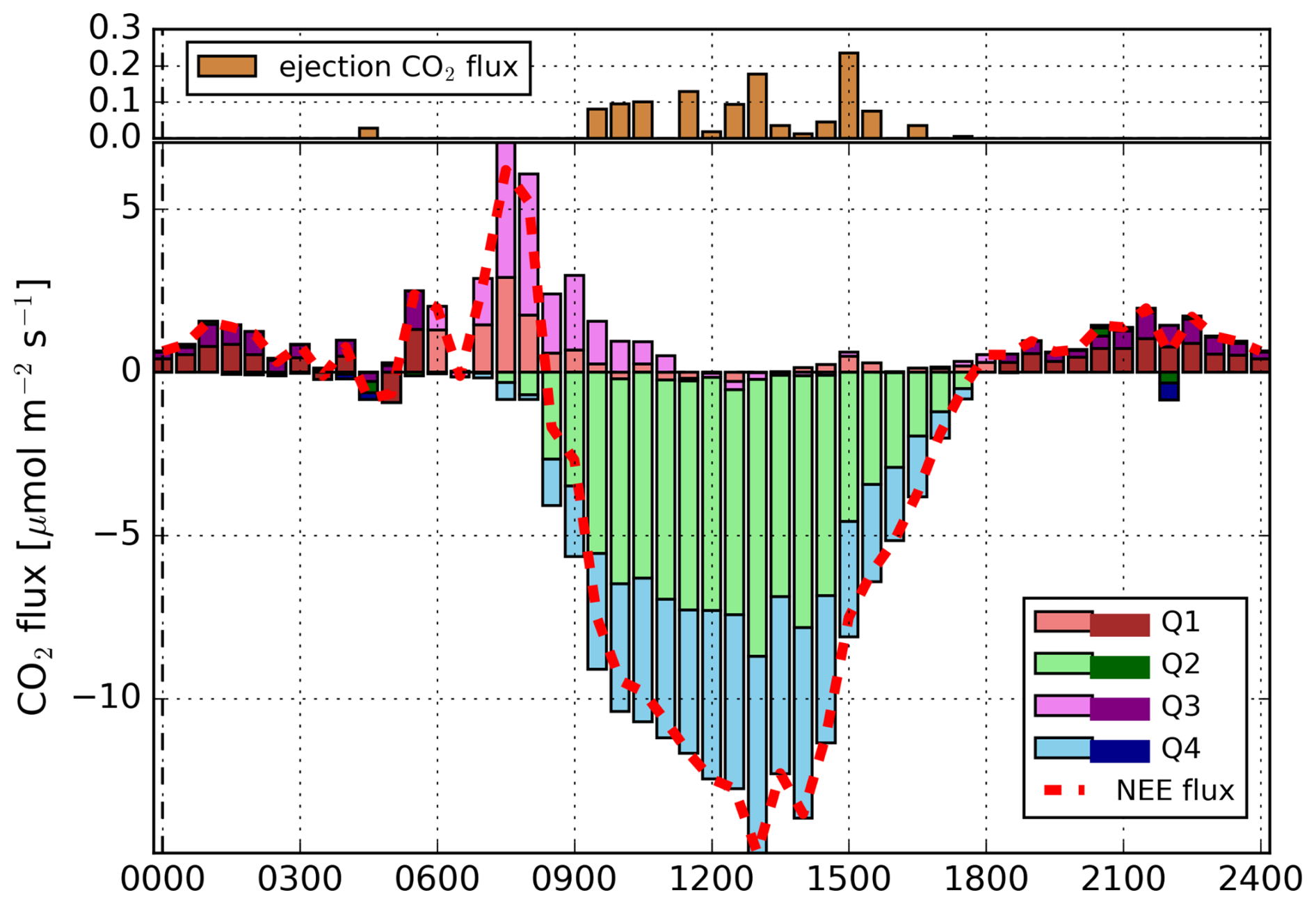
Figure 2 Composite diurnal cycle of the CO₂ NEE flux derived using quadrant analysis. The 30 min flux data are based on EC measurements taken from 8 to 21 August at 57 m. The quadrant analysis of fluxes is described in Sect. 2.1. The dashed red line is the sum of all quadrant contributions, which equals the NEE flux. The darker colours indicate the night-time hours. The ejection fluxes in the top subpanel were calculated analogously to the quadrant fluxes, using Eq. (1), only employing the ODR “ejection” and “bulk” partitioning to specify the data subsets. Figure A7 shows the quadrant analysis of H₂O fluxes.

2.2 Isotopic source compositions

We use the Miller–Tans method (Miller and Tans, 2003) to derive source compositions from 30 min intervals of 4 Hz H₂O, δ¹⁸O-H₂O, and δD-H₂O data. To limit errors in the source compositions of ejections, we only derived source compositions when at least 36 ejection data points were present (from a total n of 7200 in 30 min). The Miller–Tans method relies on fitting a line, of which the slope represents the isotopic source composition. We excluded cases in which the standard error of this slope, following the error propagation described York (1968), was larger than 6 ‰. We also excluded physically unrealistic source compositions that fell outside the range −20 ‰ to 70 ‰. We speculate that, in such cases, the mixing assumptions underlying the Miller–Tans were violated due to the advection of air masses with different compositions.

The limited number of data points available for finding the ejection could force derived source compositions to zero due to the nature of some regression fitting algorithms. To prevent this, we used the York regression fitting algorithm recommended in Wehr and Saleska (2017), which incorporates the uncertainties in x and y, to apply a linear fit to the data (York, 1968). Moreover, we verified that our results were not biased due to fitting issues, by confirming that a subset of bulk exchange data points, matching the ejections with respect to the number of points and y range, still resulted in a similar isotopic source composition compared to all bulk data points (see Fig. A3). The CO₂ isotope laser spectrometer was too unstable for the derivation of source signatures. Leaf and soil samples were analysed for water stable isotopic composition following (Barbeta et al., 2019). In Appendix A1, we detail our sampling approach and isotopic analysis method.

2.3 Cloud time-shifting

The relation between cloud passages and ejections was investigated using lower-frequency (10 s average) data from the 10:00 to 16:00 interval. We define the “understory ejection intensity” as the fraction of time in the 10 s interval during which air parcels were classified as understory ejections. We used an incoming photosynthetic active radiation (PAR) sensor to determine when and for how long clouds passed. PAR and EC data were collected at 20 Hz on one data logger, ensuring time synchronisation. A “cloud intensity” variable was derived by calculating the percentage decrease in the measured PAR relative to a calculated clear-sky PAR curve. Clouds that caused less than 10 % radiation dimming or lasted less than 20 s were excluded. The first interval during which a cloud was observed is referred to as the cloud onset. In total, 518 clouds were identified during the measurement period. A total of 69 lasted for more than 4 min, and we refer to these clouds as “big clouds” (cloud size >1 km given the 3.9 m s⁻¹ U_avg,57 m at ATTO).

To find a temporal relationship between clouds and ejections, we applied time-lagged cross-correlation to the “understory ejection intensity” and “cloud intensity” variables. With a characteristic timescale of active cumulus clouds of around 20 min and assuming cloud effects to be limited to 5 min before and after a cloud, we selected a 30 min time-shift interval for this cross-correlation (Romps et al., 2021). Coherent positive correlation coefficients should indicate if clouds trigger ejections, and the time of maximum cross-correlation specifies at what time lag that relationship is strongest (Fig. 4).

We also determined the distribution of ejections around the onset of clouds. To prevent assigning one ejection to multiple clouds, all ejections were first assigned to the closest cloud onset in time. Then, we cumulatively added all ejections that occurred in a given time window around the start of each cloud. A consequence of analysing at the closest ejection occurrence is that randomly generated cloud and ejection fields are correlated too (see Fig. 4). This issue is further discussed in Sect. 3.4 and visualised by the synthetic data in Fig. 4c.

3 Results

3.1 CO₂ and H₂O turbulent transport: quadrant decomposition

Figure 1 shows the anomalies in CO₂ (x axis) and H₂O (y axis) associated with the bulk turbulent exchange, measured in the atmospheric boundary layer (ABL). Each data point in panels (a), (b), and (c) is the deviation of a 10 Hz observation relative to the 30 min mean, colour-coded by the associated instantaneous vertical wind speed. Figure 1a shows a representative daytime 30 min interval (convective turbulent conditions with scatter clouds), where a negative correlation between H₂O and CO₂ is observed. Air parcels with upward motions shown in red are characterised by anti-correlated reduced mole fractions of CO₂ and increased H₂O mole fractions resulting from the opposing CO₂ assimilation and transpiration flux directions. Downward motions in Q₄ instead originate from the atmosphere above. See Fig. A5 in the Appendix for a u^′–w^′ plot as defined by Shaw et al. (1983).

Figure 1b shows a 30 min night-time example (stable stratification above the canopy, probably mechanical turbulence) in which we find a positive correlation between H₂O and CO₂. The pattern is a consequence of the combined CO₂ soil and plant respiration and evapotranspiration that feeds both CO₂ and H₂O into the atmospheric background shown in Q₃. Vertical motions during the night are weaker compared to those during the day, with maximal 30 min perturbations in w^′ ranging from 0 to 0.5 m s⁻¹.

Similar to Fig. 1a, Fig. 1c shows a daytime example. Here, however, a prominent streak of data points deviating from the bulk trend is observed in Q₁. This upward-moving (red colour) air mass must originate from a humid and respiration-dominated part of the biosphere, which can only come from the shaded understory. Therefore, we classify these streaks as understory ejections. The u^′–w^′ quadrant defined by Shaw et al. (1983) would categorise every understory ejection data point, as well as many others, as wind ejections (Fig. A5). Using the understory separation as described in Sect. 2.1, we isolated the occurrences of understory ejections based on the fitted dashed blue line. The ejection episodes identify the upward transport of understory air that is enriched in both CO₂ and H₂O and moves through the canopy crown and into the ABL, as observed at the 54 m measurement location. Most 30 min flux intervals did not display understory ejections; however, if they did, they generally contained fewer data points and less extreme mole fraction anomalies compared to this example case. Detailed evaluation of the example in Fig. 1c shows that the streak of data points mostly represents two updraught events lasting for tens of seconds each (Fig. A1).

Figure 1d shows the diurnal distribution of all observed ejections. While contributions varied, ejections were observed during all 13 d. They occurred during most daylight hours and were most intense around 15:00 LT. This coincides with larger cumulus clouds developing, as confirmed by previous studies and by webcam footage captured at the site (Tian et al., 2021). The coherence in the anomalies in CO₂ and H₂O reveals that these ejections around 15:00 LT are part of a second phase of ejections. The first phase (09:00–10:30 LT) is associated with a remnant of the morning transition, which is characterised by the flushing up of air that was trapped within the canopy during nocturnal stability (Dupont et al., 2024). The bulk of the flushing takes place from 07:00 to 09:00 LT, but the positive relationship between the H₂O and CO₂ anomalies prevents ejection events from being isolated to this time period (Fig. 2). Therefore, we only observe ejections in phase 1, after photosynthesis has become dominant around 09:00 and until the night-time respiration residuals have mixed up at 10:30. It is possible that the “merging phase” of the residual layer from the day before and the newly developing convective boundary layer, as described in Spiridonov and Ćurić (2021), are associated with the ejection-lean period at 10:30, between both phases. Wind direction analysis of all understory ejections suggests that ejections did not emerge under a preferential wind regime (Fig. A2).

3.2 Quadrant analysis of CO₂ fluxes

Figure 2 shows a 13 d average diurnal cycle of the 30 min CO₂ NEE flux. The colours indicate the contribution from each of the four H₂O and CO₂ quadrants (Sect. 2.1). The top pane displays the vertical fluxes of the ejection events within each 30 min interval. From 09:00 to 17:00, flux contributions from ejections occur sporadically. Over the 13 d campaign period, ejection contributions to the flux summed to 1.4 % of the total NEE in absolute terms. Within 30 min flux intervals, ejection contributions regularly reached 20 %. On average, when ejections were observed in an interval, they contributed 3.8 % to the flux.

At 07:30, NEE is most positive, meaning that there is bulk transport of CO₂ from the canopy towards the ABL. Q₁ and Q₃ contribute equally, where Q₁ represents upward transport of air influenced by accumulated respiration from the soil and the entire canopy, whereas Q₃ represents the downward transport of air masses with low CO₂ and H₂O contents. Simultaneously, photosynthesis becomes active, counteracting the upward CO₂ flux (Vilà-Guerau de Arellano et al., 2024).

From 09:00 onward, Q₂ and Q₄ dominate the bulk transport because the photosynthesising canopy now controls the gas exchange (Fig. 1a). Around noon, the CO₂ canopy uptake flux is largest. During that time, 12 % of data points in the CO₂–H₂O space are data points anomalous from the bulk exchange because they fall into Q₁ and Q₃ (see Fig. 1a). This percentage decreases over the course of a day as increased mixing makes the boundary layer more uniform with respect to the state variables and atmospheric composition. At noon, the downward CO₂ flux caused by these anomalous bulk data points is partially counteracted by the upward understory ejection flux, which exists in Q₁ (upper panel in Fig. 2). The result is a near-zero net flux in Q₁ and Q₃ at noon (lower panel in Fig. 2).

At 15:00 LT, only 6 % of data points are anomalous, as the H₂O–CO₂ relationship is tighter (well mixed; see Fig. 7 and D₁ in Vilà-Guerau de Arellano et al., 2024). As a consequence, we observe a net upward flux of CO₂ in Q₁ that correlates with the number of ejections (see Fig. 1d). The same can be seen in Q₁ and ejection fluxes of the H₂O quadrant fluxes (Fig. A7).

During the evening transition (18:00 onward), the fluxes in all quadrants are close to zero, followed by a steady respiration signal in Q₁ and Q₃ throughout the night. Increased horizontal and vertical heterogeneity in combination with suppressed vertical motions in the stable nocturnal boundary layer above the canopy result in a noisy flux signal.

3.3 Source identification

High-resolution measurements of the water vapour isotopic composition are used to compare the isotopic composition of the understory ejections with that of the bulk exchange (Griffis, 2013). Both δD and δ¹⁸O were measured, but we focus on δD because of a higher signal-to-noise ratio. Figure 3a shows isotopic source signatures from a Miller–Tans plot analysis, which reveals a consistently depleted source isotopic composition for the isolated understory ejections compared to the bulk exchange. Representative examples of Keeling and Miller–Tans plots are shown in Fig. A4 (Keeling, 1958; Miller and Tans, 2003). The understory source composition has a larger uncertainty due to the limited number of data points and the small range in the H₂O mole fraction, but this does not explain the difference (see Sect. 2.2).

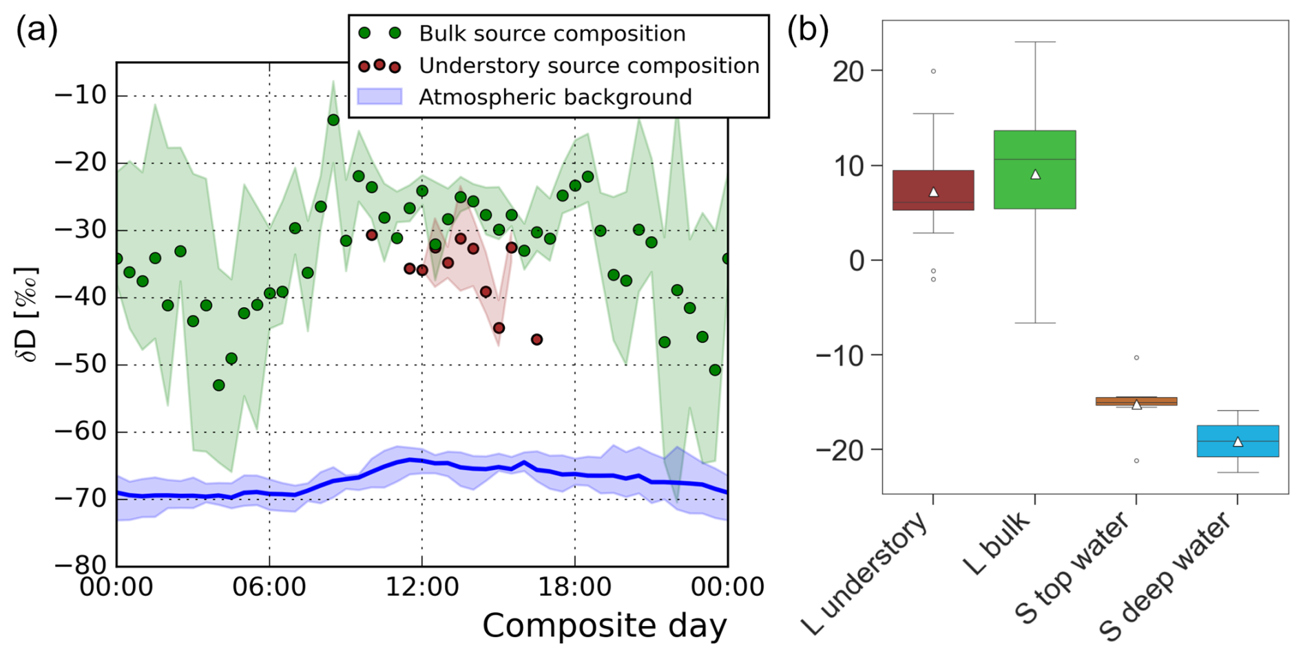
Figure 3 Diurnal δD isotopic source signatures derived from Miller–Tans plots. Each symbol represents a 30 min data interval averaged over the period from 8 to 21 August 2022. Understory contributions (brown symbols) can only be calculated for the period with frequent ejections (Fig. 1d). Note that the emitted water vapour is always isotopically enriched relative the ambient isotopic composition (blue). Leaf (L) and soil (S) liquid water samples shown in panel (b) were collected over 3 d during the 13 d campaign (Appendix A1). Only leaf samples collected between 11:00 and 17:00 were used. The triangles represent the mean.

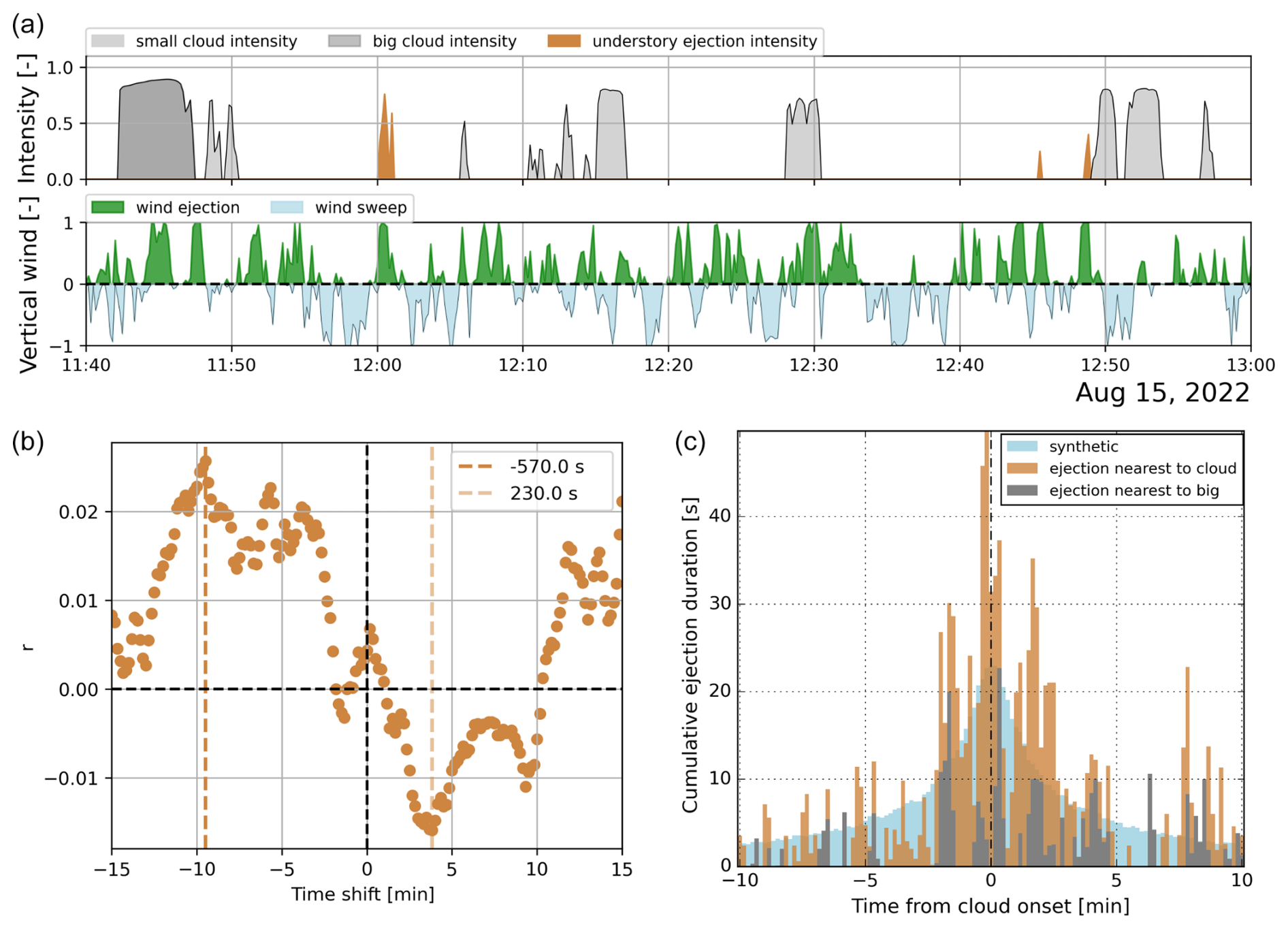
Figure 4 (a) An example afternoon period from 15 August with many clouds, some understory ejections, and wind sweeps and ejections in the vertical wind panel. Clouds were identified using the difference between clear-sky PAR and observed PAR. Big clouds were those that lasted for more than 4 min, which corresponds to a cloud size of about 1 km horizontally. Wind sweeps and all ejections are displayed as the fraction of time that an ejection occurred during the 10 s interval. (b) The cloud–ejection relationship when time-shifting the data series by 10 s intervals. The vertical lines identify the maximum and minimum correlation between the “cloud intensity” (small and big) and “understory ejection intensity” variables. (c) The cumulative distribution of ejections around cloud onsets using 10 s bins. Data ranged from 09:00 to 16:30 during the 8 to 21 August 2022 period.

The source signature for bulk exchange reflects canopy–air interactions (Welp et al., 2012). Looking at the daily changes in isotopic composition, a clear diurnal cycle emerges (Fig. 3). After sunrise at 06:03, the depleted night signature enriches, peaking at 08:30, most likely because of dew evaporation and leaf transpiration (Cernusak et al., 2016). A stable midday plateau ends post-sunset at 18:04, followed by a decline to more depleted night values, indicating water re-equilibration (Cernusak et al., 2016). Note that the uncertainty in the source signatures is high during night-time. Still, events with more depleted source compositions occur at 23:00 and at 04:00 in this composite diurnal cycle, where the 04:00 event is possibly related to dewfall (Li et al., 2023).

During the midday plateau (09:00–17:00 LT), sufficient ejections (Fig. 1d) allow for a reliable determination of the understory source composition (Fig. 3a). Here, a consistent deuterium depletion in understory ejections is observed compared to the bulk exchange. Differences can reach up to −10 ‰ between 14:30 and 15:30. Figure 3b shows the midday isotopic compositions of leaf and soil samples taken at different heights/depths. We find that shaded understory leaves and topsoil water, from which evaporation takes place, are isotopically depleted compared to bulk sunlit leaves (predominant at the canopy top). This is in agreement with previous studies (Cernusak et al., 2016). An ANOVA test indicates that the depletion of understory leaves compared to bulk leaves is not significant for our sample (p=0.34). The Craig–Gordon model was used to determine the isotopic composition of the liquid water at the exchange site (δ_e), as a function of the isotopic composition of atmospheric water vapour (δ_a), the source water (δ_s) of the plant, and environmental variables (Appendix A3). In line with our understanding, it suggests that the δ_e of leaves from the bulk canopy is 20 ‰ more enriched compared to the leaf water average derived from our sample (Cernusak et al., 2016). In addition, the δ_e of understory leaves is depleted by 1.9 ‰ compared to the leaves from the bulk canopy. This supports the idea that understory leaf water is comparatively depleted too. The 10 ‰ deuterium depletion of understory source air in Fig. 3 cannot qualitatively be explained by a ≈2 ‰ depletion in leaves only. Liquid water in the soil is about 20 ‰ depleted compared to leaf water (Fig. 3b); thus, evaporated vapour from the soil should have a similar depletion of 20 ‰ compared to transpiration from leaves. We can, therefore, expect that contributions from soil evaporation, which contribute to the understory source air, explain the 10 ‰ depletion that we find.

Plant source water is the average of the water in the root zone, which can be sampled from the plant xylem (de Deurwaerder et al., 2020). We approximate the isotopic composition of the source water by taking the average of the deep soil samples (−20 ‰) and a sample taken from a stream draining the local plateau (−27.4 ‰ at ≈ 70 m lower elevation). This approximation is supported by (1) the fact that plant water uptake does not cause isotopic fractionation and (2) the knowledge that horizontal and vertical water isotopic gradients are limited in a rainforest with excess precipitation (Rothfuss and Javaux, 2017; Vega-Grau et al., 2021). We find that our plant source water (−23.7 ‰) closely resembles the daytime bulk evapotranspiration source (−25 ‰), which confirms the isotopic transpiration equilibrium in plants (Yakir and da Silveira Lobo Sternberg, 2000)

3.4 Inferring cloud–ejection relationships

Figure 4a shows an 80 min period in which a period of ejections coincides with cloud passages. We find that understory ejections of CO₂ are strongly associated with wind ejections, which are displayed in the bottom subpanel. The ejection at 12:49 LT occurred in close proximity to a cloud onset. We expect ejections and clouds to be temporally correlated, as clouds have the potential to break the in-canopy stability radiatively and/or dynamically (Fitzjarrald et al., 1988; Machado et al., 2024). Increased wind dynamics are caused by the large convective structures associated with clouds. Additionally, the shading provided by the clouds yields a horizontal temperature gradient that triggers small-scale circulations above the canopy top (Horn et al., 2015). Our complete dataset comprises 13 d and contains 518 clouds and 379 ejections of different intensities.

Figure 4b shows the time-lagged cross-correlation between the cloud intensity and ejection intensity (Sect. 2.3). Negative and positive x coordinates represent the periods before and after the centre of clouds passing, respectively. Note that the focus on the cloud centre is not a choice but, rather, a feature of the time-lagged cross-correlation. At x=0, which represents ejections occurring during the centre of a cloud passage, no correlation is observed with understory ejections. An increased probability of ejections is observed for negative time shifts, i.e. prior to the cloud centre's arrival, with higher correlation coefficients for time shifts between −11 and −3 min. This suggests that relatively important dynamic and radiative effects occur before or at the start of the cloud triggering an ejection. We note that, while the correlation is coherent, the correlation coefficients are low (r<0.03). An important cause of this is that many clouds and ejections occur in isolation (see panel a). Another factor is that we correlate an intermittent ejection time series with a smooth, block-shaped cloud time series. While we find a temporal link between clouds and understory ejections, clouds of all characteristics (density and size) are included, making it unclear where ejections occur with respect to the cloud onset or which cloud size predominantly contributes.

A second approach was used to determine the ejection timing relative to cloud onsets (Sect. 2.3). In this approach, we investigated the cloud onsets instead of the centres and accumulated all ejection occurrences around those cloud onsets. We found that 23 % of clouds had one or more ejections in the 20 min window around their onset, while 66 % of ejections occurred within these same windows. This effect is caused by the clustered occurrence of ejections compared to the distributed nature of cloud fields (Romps et al., 2021). Figure 4c only shows the ejection events in the 20 min window closest to the cloud onset, accumulated over “all” or “big” cloud cases.

To visualise the bias associated with only selecting the closest events, the blue bars show a synthetic ejection distribution. Here, we applied a time shift of at least 1 h to the cloud field compared to the real measurement, and this differed by 15 min between synthetic samples. Ultimately, each ejection gets co-located with 379 unrelated cloud fields. The synthetic data in Fig. 4c are the average histograms over these 379 runs. Only data from the 09:00–16:30 period, during which ejections are present, were used. In the 4 min window around the 0 min offset, the cumulative ejection duration (y axis) of the observed time series much exceeds the synthetic background, suggesting that more ejections were present during cloud onsets then chance allows. While the pattern is noisy, an F test confirms a significantly tighter distribution for “all” clouds than for the synthetic data (p=0.02). This supports the idea that ejections preferentially take place near cloud onsets and, thus, before the centre of a cloud. The distribution of the “big” cloud cases is not significantly tighter compared to the synthetic background.

4 Discussion

Our analysis demonstrates that fractions of trapped understory air regularly manage to escape through the canopy crowns towards the ABL (Fitzjarrald et al., 1988; Jacobs et al., 1992; Pedruzo-Bagazgoitia et al., 2023). These understory ejections present a small but measurable contribution to the NEE flux (1.4 %). Time-averaged in-canopy profile data from González-Armas et al. (2025) confirm that a disconnected understory layer was also present during our measurement campaign. In terms of composition, we use anomalous increases in the H₂O and CO₂ mole fractions to identify understory ejections. In turn, we find distinctly moist and CO₂-rich air coming from the understory. Interestingly, understory ejections were found to be associated with depleted water vapour isotopic compositions compared to vapour arising from bulk canopy transpiration. A depletion in the understory is supported by the difference in the isotopic composition of water in sunlit leaves, shaded leaves, and the topsoil (Fig. 3b), confirming previous studies (Yakir and da Silveira Lobo Sternberg, 2000; Cernusak et al., 2016). Furthermore, we show that the isotopic composition of the bulk transpiration source is of similar isotopic composition to the deep soil water.

While we verified the hypothesised relationship between clouds and ejections, this relationship was not as strong as anticipated. We regularly observe ejections that are not associated with clouds causing PAR shading. All understory ejections are linked to strong updraughts, which have been described here as wind ejections (Fig. A5). Through the effect of wind shear, a negative correlation between horizontal winds (U) and understory ejections was also found when considering 10 s intervals. In Fig. A6, we investigated if period with stronger wind gusts were related to periods with more ejections. In this way, we bypassed the dependence of wind and understory ejections on short timescales. When limiting our analysis to daytime intervals (09:00–16:30), we found no significant relationship between gusty and ejection-rich periods.

An advantage of our method for establishing cloud–ejection relationships is that we reduce the complexity of the 4D spatiotemporal observational space to a 1D point measurement, including detailed insight into the local atmospheric composition. This means that factors like wind direction and wind speed, which would strongly effect and complicate displaced measurements, drop out. As long as the wind direction remains similar over time and over the height of the boundary layer, an ejection triggered at some distance from the tower – and the cloud that caused it – are synchronously observed by the measurement station (Taylor's frozen-turbulence hypothesis). Some uncertainty is caused by our use of cloud shadows, which introduce unwanted horizontal displacements due to the varying zenith angle. Strong wind shear may also cause some uncertainty, as it will offset the arrival of cloud and composition data.

Finding a stronger causal mechanism triggering the observed understory ejections should have priority. To this end, better cloud data spatially co-located (<10 m) with wind and composition data at a forest site are needed (Machado et al., 2024). More advanced cloud observational techniques, like cloud radars or ceilometers, would provide 3D spatiotemporal information, but these instruments are hardly portable and are preferably installed on bare soil, limiting their use in forest environments. Webcams combined with cloud recognition analysis tools could provide a possible alternative.

With a more clear characterisation of the trigger mechanism leading to understory ejections (Machado et al., 2024; Patton et al., 2016), the rapid development of canopy-resolving large-eddy-simulation models could be validated (Pedruzo-Bagazgoitia et al., 2023; Dupont et al., 2024). Moreover, multilayer canopy representations have shown to improve the next-generation Earth system models (Bonan et al., 2024).

5 Conclusions

We have used high-temporal-resolution measurements of CO₂ and H₂O above the canopy of the Amazon rainforest, combined with innovative analysis techniques, to investigate the intermittent interactions between the dry-season rainforest and the dynamics of the atmospheric boundary layer. CO₂–H₂O quadrant plots allowed us to dissect photosynthetic and respiration-dominant exchange modes. Understory ejections, which transport air masses that have been in direct contact with the soil and the lower canopy, can be found in turbulent quadrant Q₁ of such a plot. These intermittent, canopy-penetrating motions constitute 1.4 % of the total CO₂ NEE flux, which matches the energy-limited understory conditions. The isotopic composition of the ejected understory air confirms that soil and plant water evaporation accumulated in the understory is depleted compared to water evaporating from the tree crowns. Clouds seem to act as a weak trigger for ejection events, but our findings are inconclusive about the dominant cause of the breaking of the canopy layer stability, which triggers ejections events. Future studies investigating understory ejections should attempt to find a causal trigger mechanism for understory ejections; this can likely be achieved using tightly co-located (<10 m) wind, scalar, and advanced cloud observational data.

Appendix A

A1 Leaf and soil sample analysis

Soil and leaf samples were collected systematically throughout daylight hours on 14 and 15 August 2022. Soil samples were collected at four locations approximately 20–100 m from the base of the 80 m tower. Once a day between 07:00 and 10:00, soil from 0–10, 10–20, 40–50, and 80–90 cm was sampled using a corer at each of the four locations. Additionally, a sample from 0–10 cm was collected with a trowel at the location closest to the tower at 07:00, 10:00, 14:00, and 16:00 on both days. All soil samples were stored in 20 mL glass vials with positive insert caps. An additional core sample was also taken from the closest location at 14:00 on 13 August 2022. Finally, a water sample was taken from the stream located at a 70 m lower elevation; this stream drains the local plateau on which the measurement tower is situated.

Leaf samples were collected at approximately 07:00, 10:00, 14:00, and 16:00 on 14 and 15 August 2022 from trees near the bottom of the tower (≈ 2–3 m), those accessible from the middle of the tower (≈ 12–15 m), and from trees at the top of the tower (≈ 24–28 m). During each sampling, leaves were collected from three trees. Similarly, additional samples were collected from all heights at between 06:00 and 15:00 on 12 August. All leaf samples were stored in gas-tight 12 mL glass vials. Samples were stored at 4 °C prior to further processing.

Soil and leaf water was extracted via cryogenic vacuum distillation (West et al., 2006) at the Instituto National de Pesquisas da Amazônia (Manaus, Amazonas, Brazil). Briefly, the system consisted of four GL 18 glass extraction vessels and U traps connected to a vacuum pump via a manifold and shut-off valve. Sufficient sample material to extract approximately 2 mL of water was weighed and transferred to extraction vessels. The samples were frozen in a dewar containing liquid nitrogen, and the shut-off valve was opened to evacuate the system. The shut-off valve was then closed, the extraction vessels were transferred to a water bath, and the U traps were moved into the liquid nitrogen. The water bath was set to approximately 90 °C, and extracted water was collected over the course of 2 h to ensure complete transfer between the sample and the U trap. Subsequently the U traps were removed and capped, and the collected water was allowed to thaw before being transferred to 2 mL plastic vials with positive insert caps. The extraction vessels and the samples that they contained were then oven-dried to verify that there was no residual water.

The isotopic composition of the extracted water was measured on a Thermo Delta Plus XL isotope ratio mass spectrometer (IRMS) coupled to a high-temperature conversion reactor (HTC) via a ConFlo III at the Max Planck Institute for Biogeochemistry, Jena, Germany (Gehre et al., 2004). Calibration was carried out relative to two in-house water standards and a quality control tied to VSMOW-SLAP (where SLAP denotes Standard Light Antarctic Precipitation). Based on tests with 2 mL of water in place of sample soil and leaf material (n=22), the average biases associated with the extraction system and analysis for δ¹⁸O and δD were $-\mathrm{0.27}\pm \mathrm{0.26}$ ‰ and $-\mathrm{3.47}\pm \mathrm{1.77}$ ‰, respectively.

A2 High-frequency water vapour isotope calibration

The Picarro L2130-i was calibrated for δD and δ¹⁸O as described in Moonen et al. (2023). In short, we used one liquid water standard to apply a mole fraction calibration. Here, we determine the sensitivity of the instrument to variations in atmospheric water content on the isotopic signals. By adding the vaporised liquid water standard to a dry (synthetic air) stream in different proportions, we simulated such atmospheric water vapour changes, while keeping the inserted δD and δ¹⁸O compositions constant. When the measurements did return a varying δD and δ¹⁸O composition, we corrected for that.

A second calibration method was used to find the absolute offset between the measurement and the known composition of water standards. To this end, two liquid water standards from the International Atomic Energy Agency (IAEA) were used that spanned the range of observed atmospheric isotopic compositions (IAEA, 2017): one was w34 ($\mathit{\delta }\mathrm{D}=-\mathrm{189.48}$ ‰ and ${\mathit{\delta }}^{\mathrm{18}}\mathrm{O}=-\mathrm{24.78}$ ‰) and the other was w39 ($\mathit{\delta }\mathrm{D}=+\mathrm{25.44}$ ‰ and ${\mathit{\delta }}^{\mathrm{18}}\mathrm{O}=+\mathrm{3.63}$ ‰). The calibration approach was a span calibration, with a H₂O set point of 15 000 ppm.

Given that the instrument is very stable over time, we used the average of the initial and final calibrations at ATTO, which were performed using the IAEA standards. Calibrations during the measurement campaign were also performed, which we used to confirm the stability. As these were made using different water standards, the compositions of which were less certain, we did not use them in our analysis. For the CO₂ isotope analyser (Aerodyne TILDAS-CS), we did need all of the 20+ additional calibrations made during the campaign. However, even then we were not able to satisfactorily calibrate the instrument. Thermal instability was the main cause of the instrumental drift, which was not sufficiently eliminated by Aerodyne's field enclosure.

A3 Craig–Gordon model

The Craig–Gordon model, first suggested by Craig and Gordon (1965), allows for the liquid water isotopic composition at the evaporation sites within leaves to be estimated. The enrichment of liquid water at the exchange site, resulting from the faster evaporation of light isotopologues, is related to the water isotopic composition found in leaf samples (shown in Fig. 3b) (Cernusak et al., 2016). In addition, the source isotopic composition of transpiration is dependent on the exchange site water isotopic composition. Generally, variants of the Craig–Gordon model are used that assume an isotopic steady state between the source (xylem) water and the isotopic composition of transpiration. Farquhar et al. (2007) provides an updated formulation of the Craig–Gordon model, which we implemented and define below.

$$\begin{array}{}\text{(A1)}& {\displaystyle }{\displaystyle }{\mathit{\delta }}_{\mathrm{e}}={\mathit{\alpha }}^{+}\left[{\mathit{\alpha }}_k({\mathit{\delta }}_{\mathrm{s}}+\mathrm{1})\left(\mathrm{1}-{\displaystyle \frac{w_a}{w_i}}\right)+({\mathit{\delta }}_v+\mathrm{1}){\displaystyle \frac{w_a}{w_i}}\right]-\mathrm{1}\end{array}$$

As we did not have access to leaf temperature measurements, we approximated $\frac{w_a}{w_i}$ with the relative humidity (RH), which is dependent on the air temperature instead. We combine data from our work with ecophysiology and profile measurements from our colleagues, which were also taken during the CloudRoots-Amazon22 campaign (González-Armas et al., 2025, their Figs. 2 and 3). A 14:00 case from a full-campaign data composite was analysed. The key variables derived from either the data composite or the literature are displayed in Table A1. We find that the exchange site liquid water (δD_e) is 1.9 ‰ more enriched in leaves at the canopy top compared to in the understory.

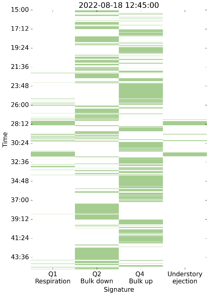
Figure A1 The temporal evolution of the quadrant contributions from Fig. 1c. The green colours specify moments when data points were part of a specific quadrant or part of an ejection streak. Note that ejections were predominantly observed in Q1.

Bonan, 2002Horita and Wesolowski, 1994Farquhar et al., 1989

Table A1 Overview of the key variables related to the Deuterium isotopic composition across the Amazon ecosystem. The results of the implementation of the Craig–Gordon model are included.

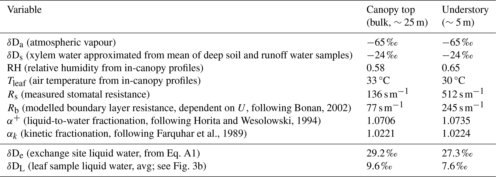
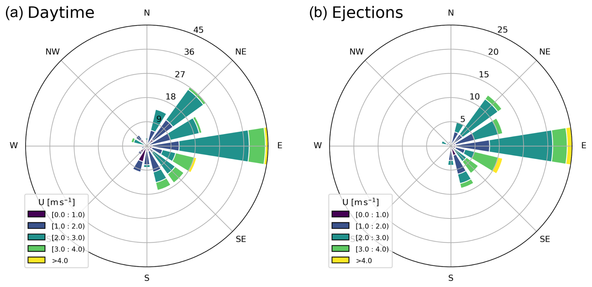
Figure A2 Wind roses of wind speeds and directions. In panel (a), all 30 min averaged wind directions observed between 09:00 and 16:30 are plotted, while in panel (b), a subset of 30 min averaged wind directions, from intervals in which ejections were observed, are plotted. The numbers on the diagonal indicate the number of data points in each wind direction bin. The result suggests that it is unlikely that a point source emission caused the ejections that we observed; rather, it may instead be a physical feature linked to tall-forest ecosystems.

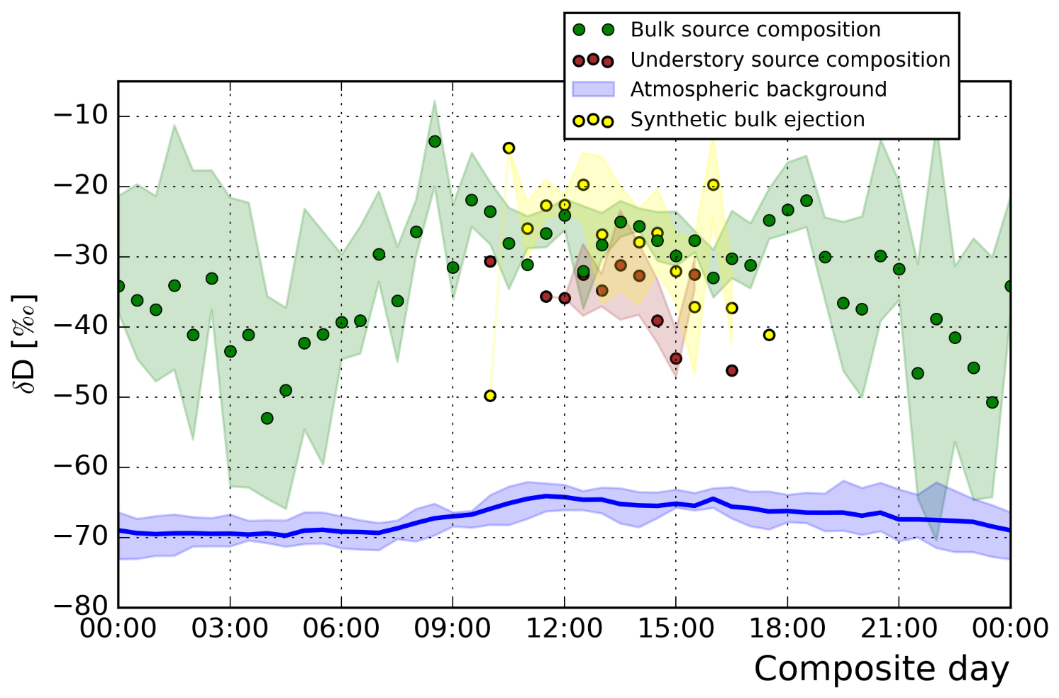
Figure A3 Source compositions derived using Miller–Tans plots. In addition to Fig. 3, in which the bulk and understory source compositions are shown, a source composition was also derived for a subset of data points from the bulk source that spanned only 25 % of the H₂O range and included as few data points as are present in small ejections (yellow marks, n=36). The result indicates that, although noise is introduced, the “synthetic bulk ejections” do not show a similarly depleted source composition to the understory ejections (see Sect. 2.2). The depletion in the understory ejection is, thus, not a feature of challenging fits with limited n but, rather, a feature related to the understory H₂O composition.

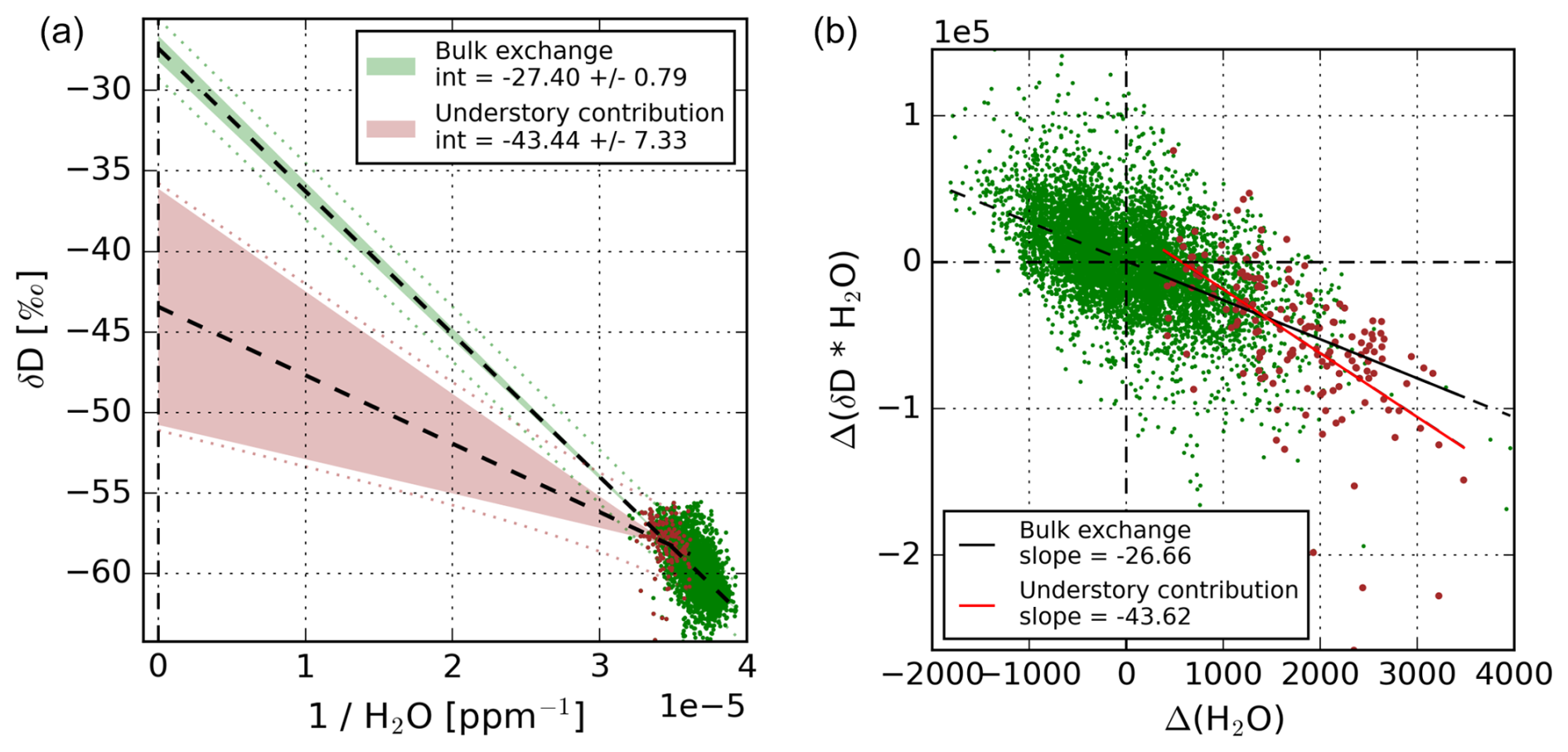
Figure A4 Example fits of the Keeling and Miller–Tans methods for finding the source isotopic composition. One 30 min example interval was used for both methods to show the differences in the resulting source compositions.

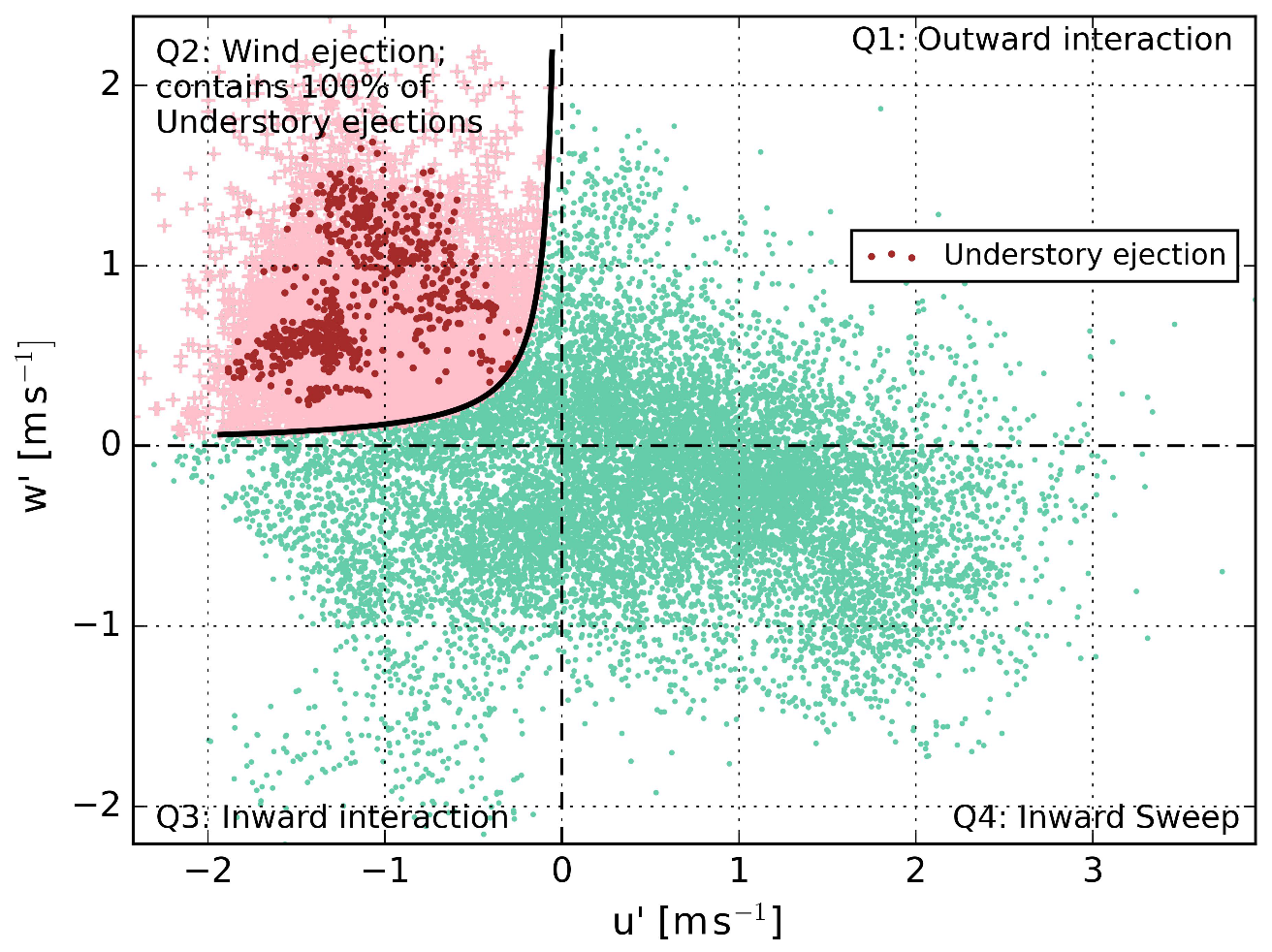
Figure A5 Quadrant analysis of the momentum flux. The black curve indicates the hyperbolic cutoff $-\mathrm{0.2}=\frac{w^{\prime }}{\mathit{\sigma }\left(w^{\prime }\right)}\cdot \frac{u^{\prime }}{\mathit{\sigma }\left(u^{\prime }\right)}$, where $w^{\prime }>\mathrm{0}$ (Eq. 2). Data that exceed this threshold are shown in pink and are considered wind ejections, as defined by Shaw et al. (1983). The example 30 min interval is the same as that shown in Fig. 1c. The red dots indicate the data points that were classified as understory ejections in Fig. 1c, Q₁. All understory ejection data points are also wind ejections. Most wind ejections, however, are not understory ejections.

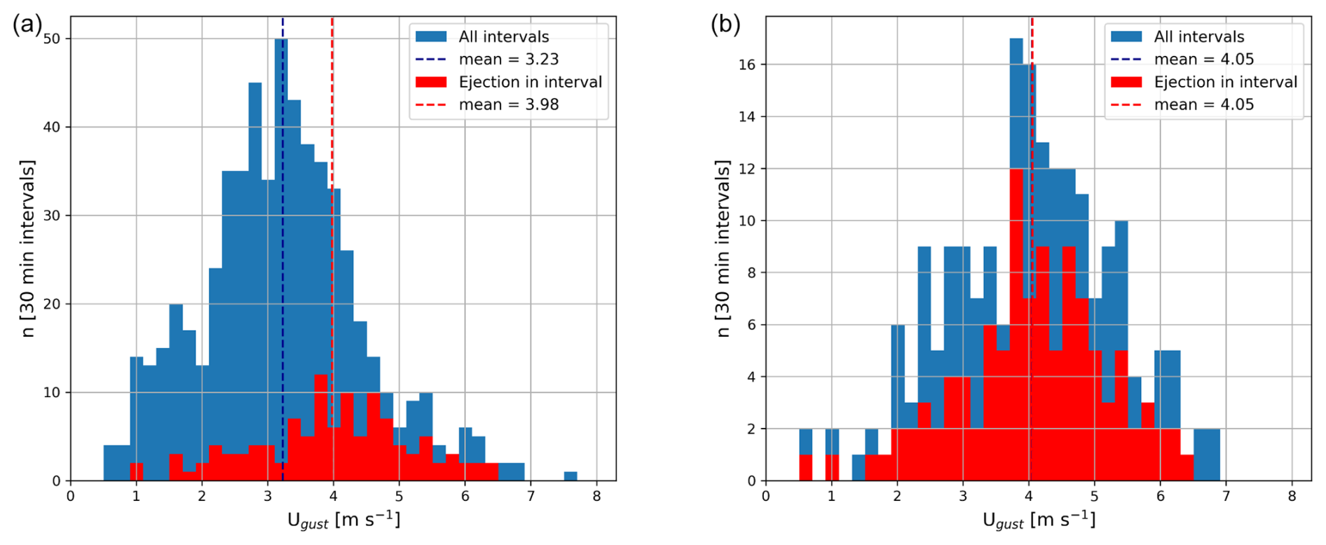
Figure A6 Distribution of the 30 min gust speeds. Panel (a) shows the result for both daytime and night-time intervals. Panel (b) is instead limited to only daytime intervals (09:00–16:30). The gust speed was determined as being the 95th percentile of 10 s U values over the 30 min interval. In red, all 30 min gust speeds during which ejections occurred are shown. A two sided t test indicates that the red and blue populations are significantly different in panel (a), with a p value of $\mathrm{4}\times {\mathrm{10}}^{-\mathrm{11}}$. The populations in panel (b) are not significantly different, with a p value of 0.48.

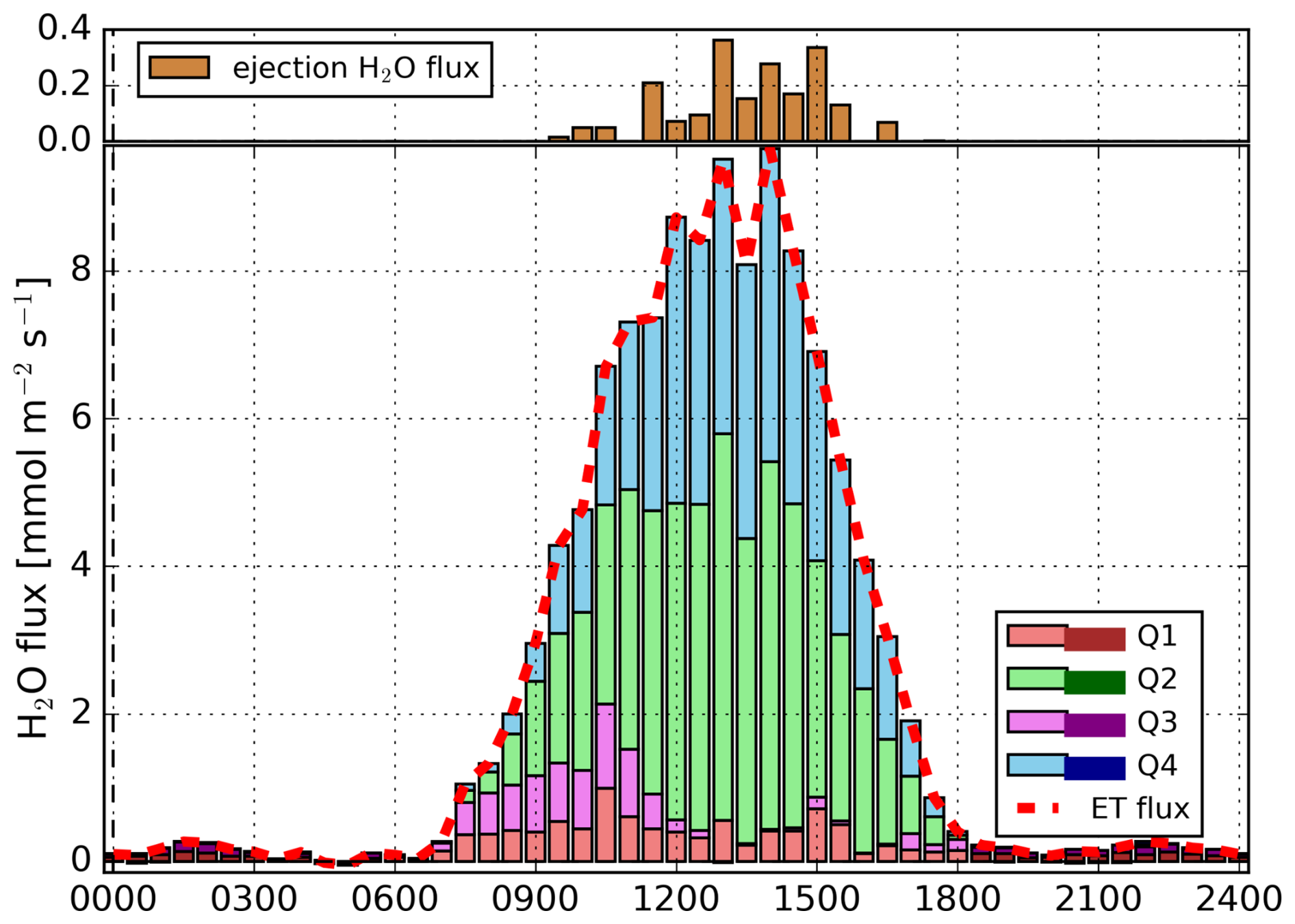
Figure A7 Composite diurnal cycle of the H₂O flux derived using quadrant analysis. The 30 min flux data are based on EC measurements taken from 8 to 21 August at 57 m. The quadrant analysis of fluxes is described in Sect. 2.1. The dashed red line is the sum of all quadrant contributions, which equals the H₂O flux. The darker colours indicate the night-time hours. The ejection fluxes in the top subpanel were calculated analogously to the quadrant fluxes, using Eq. (1), only employing the ODR “ejection” and “bulk” partitioning to specify the data subsets.