Stratospheric δ¹³CO₂ observed over Japan and its governing processes

Due to very few reports of δ¹³CO₂ (the stable carbon isotopic ratio of CO₂) observations in the stratosphere, its variations are not well understood. In order to elucidate stratospheric δ¹³CO₂ variations and their governing mechanisms, we have collected stratospheric air samples using balloon-borne cryogenic samplers over Japan since 1985 and analyzed them for δ¹³CO₂. To obtain precise δ¹³CO₂ values, we incorporated the mass-independent fractionation of ¹⁷O and ¹⁸O in the δ¹³CO₂ calculation. δ¹³CO₂ has decreased through time in the mid-stratosphere with an average rate of change of −0.026 ± 0.001 ‰ yr⁻¹ for the period 1985–2020, consistent with that in the troposphere. However, mid-stratospheric δ¹³CO₂ values did not show a time delay compared to the tropical tropospheric values. This could be explained by the production of CO₂ by CH₄ oxidation and the gravitational separation of ¹³CO₂ and ¹²CO₂. To confirm this hypothesis, we used a two-dimensional model to simulate the stratospheric δ¹³CO₂ values while accounting for these processes. The results indicate that these two effects strongly impact the vertical distribution of δ¹³CO₂. We newly defined “stratospheric potential δ¹³C” (δ¹³C_P) as a quasi-conservative parameter incorporating the kinetic isotope effect of CH₄ oxidation and gravitational separation, and we found that δ¹³C_P in the mid-latitude mid-stratosphere decreases over time with about a 5 yr lag relative to the tropical upper troposphere. This fact strongly supports that stratospheric δ¹³CO₂ variations are governed by the airborne production of ¹³C-depleted CO₂ by CH₄ oxidation, the gravitational separation, and the propagation of the decreasing tropospheric δ¹³CO₂ trend into the stratosphere.

1 Introduction

The isotopic ratio of carbon in CO₂ (here, we use “δ¹³CO₂” to distinguish it from that in CH₄, “δ¹³CH₄”) is thought to provide information on the carbon cycle, and observations have been carried out mainly using ground stations, ships, and aircraft in the troposphere (e.g., Keeling et al., 1995; Francey et al., 1995; Nakazawa et al., 1993; Morimoto et al., 2000). However, there have been very few reports of δ¹³CO₂ observations in the mid-stratosphere, mainly because of the difficulty in collecting air samples at such altitudes; the only available reports are balloon observations over Japan and Scandinavia (Gamo et al., 1995; Aoki et al., 2003). It is well known that tropospheric δ¹³CO₂ values have decreased with time due to anthropogenic emissions with low δ¹³CO₂ values resulting from fossil fuel consumption. Gamo et al. (1995) reported that δ¹³CO₂ values observed in the mid-stratosphere were higher than those in the troposphere over the same period, and that the average stratospheric δ¹³CO₂ value during 1986–1992 was about −7.5 ‰ and decreasing with time. Aoki et al. (2003) reported that the mid-stratosphere (25–32 km altitude) δ¹³CO₂ value over Japan in 1997 was approximately −7.7 ‰; this value is consistent with the expected value extrapolated from the results of Gamo et al. (1995), suggesting that their estimated secular decreasing trend is plausible.

Anomalous ¹⁸O enrichment in stratospheric CO₂ was first reported in balloon observations (Gamo et al., 1989), which spurred extended studies of the mass-independent isotopic effect (MIE) on the triple oxygen isotope system (e.g., Thiemens, 1999; Kawagucci et al., 2008). The isotopic fractionation is usually caused by the effect of mass differences between isotopologues (i.e., the mass-dependent isotopic effect). In this case, the fractionation between ¹⁸O and ¹⁶O is almost twice as large as that between ¹⁷O and ¹⁶O. However, the isotopic fractionation that does not follow this relation occurs mainly in photochemical processes. These MIE studies have clarified that the relationship between ¹⁷O and ¹⁸O enrichment in stratospheric CO₂ is quite different from that in the troposphere. This fact is very important for stratospheric δ¹³CO₂ measurements because mass spectrometry measures the ratios ⁴⁵CO${}_{\mathrm{2}}{/}^{\mathrm{44}}$CO₂ and ⁴⁶CO${}_{\mathrm{2}}{/}^{\mathrm{44}}$CO₂, and an assumed relationship between ¹⁷O and ¹⁸O enrichment is needed to calculate δ¹³CO₂. The influence of the MIE on oxygen in stratospheric δ¹³CO₂ has not been taken into account in previous studies. Although Aoki et al. (2003) found that δ¹³CO₂ values increase with increasing altitude in the stratosphere over Japan and suggested that the MIE on ¹⁷O and ¹⁸O should be considered when interpreting such a vertical distribution, no quantitative investigation of these factors has been conducted.

Stratospheric methane (CH₄) is destroyed by reactions with hydroxyl (OH), excited singlet oxygen (O(¹D)), and chlorine (Cl) radicals, and thus plays an important role in stratospheric chemistry. However, the quantitative contributions of these chemical processes to CH₄ loss and their temporal variations remain poorly understood. It is thought that δ¹³CH₄ provides useful information about CH₄ destruction in the stratosphere because characteristic isotopic fractionations occur in each reaction (e.g., Saueressig et al., 1995; Sugawara et al., 1997; Rice et al., 2003; Röckmann et al., 2011). However, only a few measurements have been made so far in the mid-stratosphere. Oxidation of CH₄ produces CO, which is eventually oxidized to CO₂. In general, the isotopic fractionations in the above reactions cause the faster destruction of ¹²CH₄ relative to ¹³CH₄, making the chemical products depleted in ¹³C (decreased δ¹³C) while the remaining CH₄ becomes enriched in ¹³C (increased δ¹³CH₄). Indeed, Brenninkmeijer et al. (1996) found that CO in the lower Antarctic stratosphere is extremely depleted in ¹³C (decreased δ¹³CO) mainly because of the local production of CO via the reaction of CH₄ with Cl. Recently, Gromov et al. (2018) and Röckmann et al. (2024) have discussed δ¹³CO variations associated with the CH₄+ Cl reaction. From these studies, it is expected that the CH₄–CO–CO₂ chain reaction could be an airborne source of CO₂ with extremely low δ¹³C values, depressing stratospheric δ¹³CO₂ values. However, no study has yet quantitatively assessed this effect.

The age of stratospheric air is the transit time of air from around the tropical tropopause to a certain location in the stratosphere, which is a powerful tool for diagnosing stratospheric transport (see Garny et al., 2024 for a review of the latest developments in air age studies). It is expected that possible changes to the Brewer–Dobson circulation induced by climate change are detectable as long-term changes in the mean age of air. For this purpose, age tracers, such as mole fractions of CO₂ and SF₆, have been measured in air samples collected by scientific balloons and satellites (e.g., Engel et al., 2009, 2017; Stiller et al., 2012). CO₂ mole fractions observed in the mid-stratosphere over Japan have been combined with SF₆ data to provide the longest record of the mean age of air, as reported by Engel et al. (2009, 2017) and Ray et al. (2014). Engel et al. (2017) reported that the mean age of air in the mid-stratosphere does not indicate a significant trend over the period 1975–2016, with only a slightly positive increase of +0.15 ± 0.18 yr decade⁻¹. However, recent models predict accelerating circulation throughout the stratosphere (e.g., Butchart, 2014), which will decrease the mean age of air. Such a decreasing trend is consistent with observational results in the lower stratosphere (Ray et al., 2014). Despite many efforts to elucidate the trend of age of air, a discrepancy remains between mid-stratosphere age trends in models and observations. One reason for this discrepancy is the large uncertainties on the observational trends. To resolve this problem, it is necessary to increase the frequency of high-altitude balloon observations and observe additional age tracers beyond CO₂ and SF₆. Perfluorocarbons and hydrofluorocarbons with extremely long lifetimes could be alternative age tracers (Leedham Elvidge et al., 2018; Laube et al., 2025; Umezawa et al., 2025), and observations of such multiple age tracers should reduce the uncertainties on mean age of air estimates.

The gravitational separation (hereafter, “GS”) of major atmospheric constituents in the stratosphere was first reported from balloon observations (Ishidoya et al., 2006, 2008a, b, 2013). They showed that vertical gradients of the isotopic and elemental ratios of major atmospheric components (N₂, O₂, and Ar) in the stratosphere are caused by molecular diffusion and depend on molecular mass. Stratospheric GS has now been observed in polar and equatorial regions (Ishidoya et al., 2018; Sugawara et al., 2018) and reproduced in numerical models (Belikov et al., 2019; Birner et al., 2020). Alongside age of air, stratospheric GS can be used to diagnose stratospheric transport processes (Ishidoya et al., 2013; Sugawara et al., 2018; Birner et al., 2020). These findings also suggest that GS could affect the mole fractions and isotopic ratios of all stratospheric constituents, although no studies have addressed the impact of GS on stratospheric δ¹³CO₂ values.

The main objective of this study is to clarify the mechanisms governing δ¹³CO₂ variations in the stratosphere and understand the long-term variations. A comprehensive understanding of the variations of stratospheric δ¹³CO₂ requires that the MIE on oxygen, CH₄ oxidation and associated isotopic fractionation, mean age of air, and GS be considered. Balloon observations provide a unique opportunity to evaluate these effects by studying a variety of atmospheric constituents using high-precision measurements. In this study, we constructed a new δ¹³CO₂ record for the stratosphere over Japan spanning the 35 yr from 1985 to 2020, primarily by newly analyzing archived CO₂ samples and in part by including previously published data (Gamo et al., 1995; Aoki et al., 2003). We then examined vertical and temporal variations in the record. Furthermore, we investigated in detail the various mechanisms affecting the vertical distribution of stratospheric δ¹³CO₂ and propose herein a new concept called “stratospheric potential δ¹³C.” We also investigated the possibility of estimating the age of stratospheric air from the δ¹³CO₂ record.

2 Experimental procedures

2.1 Air sample collection

We have collected stratospheric air samples over Japan since 1985 using balloon-borne cryogenic samplers (e.g., Nakazawa et al., 1995). A large scientific balloon equipped with a sampler was launched nearly once a year during 1985–2002 from the Sanriku Balloon Center (SBC; 39° 10^′ N, 141° 50^′ E). The frequency of observations has decreased since 2004, with the longest interval between observations being 5 yr. During this period, the balloon launch site was relocated from SBC to the Taiki Aerospace Research Field in Hokkaido (TARF; 42°30^′ N 143°26^′ E) in 2008. Balloon observations conducted so far over Japan are summarized in Table S1 of the Supplement. The cryogenic air sampler consists mainly of a liquid helium dewar, stainless steel bottles, motor-driven valves, and a control unit (Honda et al., 1996). Liquid helium was used as a refrigerant for collecting stratospheric air cryogenically under low atmospheric pressures, and 20–30 L STP of stratospheric air was collected in each bottle, depending on the altitude. Air sampling was performed typically at 11 different altitudes, spaced about 2 km apart, between 14 and 35 km altitude. Occasionally, anomalously low CO₂ mole fractions were observed, probably due to sample deterioration in the bottle. In such cases, both CO₂ mole fraction and δ¹³CO₂ data were excluded from the data record. In 2020, the CO₂ mole fraction and δ¹³CO₂ value at 28.8 and 30.9 km altitude were not available due to water contamination of the air samples.

2.2 Analytical methods for mole fractions and isotopic ratios

Collected air samples were distributed to several institutes in Japan for analysis of the mole fractions and isotopic compositions of various gases. The CO₂ mole fraction was measured using a nondispersive infrared gas analyzer at Tohoku University (TU) with an analytical precision of <0.02 µmol mol⁻¹; the CO₂ measurement protocol has been described in detail in previous studies (Nakazawa et al., 1995; Aoki et al., 2003; Sugawara et al., 2018). N₂O and CH₄ mole fractions were measured using gas chromatographs equipped with an electron capture detector and flame ionization detector, respectively, at TU. The N₂O mole fraction was used both for mass spectrometry analyses to determine δ¹³CO₂ and to investigate the MIE between ¹⁷O and ¹⁸O in CO₂, as described below. The analytical precisions for the N₂O and CH₄ mole fractions were 0.3 and 3 nmol mol⁻¹, respectively (Nakazawa et al., 2002; Aoki et al., 2003; Ishijima et al., 2007).

The analytical procedures for δ¹³CO₂ in air samples collected after 1988 have already been described in previous studies (Nakazawa et al., 1993, 1997a; Morimoto et al., 2000), and is briefly summarized here. An aliquot of each air sample (about 550 mL STP) was introduced into a CO₂ extraction system, and the pure extracted CO₂ was divided and sealed in small glass tubes; some tubes were archived for future study. The carbon and oxygen isotopic ratios (δ¹³C and δ¹⁸O) of the sample CO₂ were measured using a mass spectrometer (Finnigan MAT-δS) installed at TU against an in-house reference CO₂ calibrated to Vienna Peedee Belemnite (VPDB). The analytical precision of δ¹³CO₂ was ±0.02 ‰ (Morimoto et al., 2000). Air samples collected in 1985, 1986, 1988, and 1989 were analyzed for δ¹³CO₂ using a mass spectrometer (Finnigan MAT250) with a reproducibility of less than ±0.02 ‰ at the University of Tokyo (Gamo et al., 1989, 1995).

In this study, we modified the calculation of isotopic ratios to take into account the stratospheric MIE and GS. Hereafter, the isotopic ratios of ¹³C to ¹²C, ¹⁷O and ¹⁸O to ¹⁶O, and ⁴⁵CO₂ and ⁴⁶CO₂ to ⁴⁴CO₂ are expressed as ¹³R=n(¹³C)$/n{(}^{\mathrm{12}}$C), ¹⁷R=n(¹⁷O)$/n{(}^{\mathrm{16}}$O), ¹⁸R=n(¹⁸O)$/n{(}^{\mathrm{16}}$O), ⁴⁵R=n(⁴⁵CO₂)$/n{(}^{\mathrm{44}}$CO₂), and ⁴⁶R=n(⁴⁶CO₂)$/n{(}^{\mathrm{44}}$CO₂), respectively, where n is the amount of each isotopologue. δ¹³CO₂ is defined as

$$\begin{array}{}\text{(1)}& {\mathit{\delta }}^{\mathrm{13}}{\mathrm{CO}}_{\mathrm{2}}=\left({\displaystyle \frac{{}^{\mathrm{13}}R}{{}^{\mathrm{13}}{R}_{\mathrm{VPDB}}}}-\mathrm{1}\right)\times {\mathrm{10}}^{\mathrm{3}}\left(\mathrm{‰}\right),\end{array}$$

where ¹³R_VPDB is the known ¹³R value of VPDB (Coplen and Shrestha, 2016). The isotopic ratios ⁴⁵R and ⁴⁶R are expressed as (Santrock et al., 1985)

$$\begin{array}{}\text{(2a)}& {}^{\mathrm{45}}R{=}^{\mathrm{13}}R+\mathrm{2}{\cdot }^{\mathrm{17}}R,\end{array}$$

$$\begin{array}{}\text{(2b)}& {}^{\mathrm{46}}R=\mathrm{2}{\cdot }^{\mathrm{18}}R+\mathrm{2}{\cdot }^{\mathrm{13}}R{\cdot }^{\mathrm{17}}R+{\left({}^{\mathrm{17}}R\right)}^{\mathrm{2}}.\end{array}$$

To calculate δ¹³C and δ¹⁸O values from ⁴⁵R and ⁴⁶R, the relationship between ¹⁷O and ¹⁸O should be known, because ⁴⁵CO₂ contains ¹²C¹⁷O¹⁶O, whereas ⁴⁶CO₂ contains both ¹³C¹⁷O¹⁶O and ¹²C¹⁷O₂. The relationship between ¹⁷R and ¹⁸R can be expressed as (e.g., Meijer and Li, 1998)

$$\begin{array}{}\text{(2c)}& {\displaystyle \frac{{}^{\mathrm{17}}R}{{}^{\mathrm{17}}{R}_{\mathrm{VSMOW}}}}={\left({\displaystyle \frac{{}^{\mathrm{18}}R}{{}^{\mathrm{18}}{R}_{\mathrm{VSMOW}}}}\right)}^{\mathit{\beta }},\end{array}$$

where ¹⁷R_VSMOW and ¹⁸R_VSMOW are the known ratios of Vienna standard mean ocean water (VSMOW; Coplen and Shrestha, 2016). In measurements of tropospheric δ¹³C and δ¹⁸O, the mass-dependent relationship between ¹⁷O and ¹⁸O can be assumed, i.e., β=0.528 (Meijer and Li, 1998; Assonov and Brenninkmeijer, 2003). However, the MIE between ¹⁷O and ¹⁸O is non-negligible in the stratosphere (Gamo et al., 1995; Thiemens, 1999). Therefore, the δ¹⁷O value is essential for accurately determining the δ¹³C value in the stratosphere. Our air samples were also measured for triple oxygen isotopes, as reported by Kawagucci et al. (2008). However, δ¹⁷O measurements were not performed for all of our stratospheric samples. In such cases, the following method was applied to obtain δ¹⁷O values. The values of ¹⁷R and ¹⁸R calculated from δ¹⁷O and δ¹⁸O observed by Kawagucci et al. (2008) were fitted to Eq. (2c), and the average value of β was calculated to be 1.7 ± 0.2 using the least squares method. For samples for which δ¹⁷O was not analyzed, we used Eq. (2c) with this β value to calculate δ¹³C. By substituting Eqs. (2a) and (2b) into (2c), we obtained the following equation:

$$\begin{array}{}\text{(3a)}& \mathrm{3}{\left({}^{\mathrm{17}}R\right)}^{\mathrm{2}}-\mathrm{2}{\cdot }^{\mathrm{45}}R{\cdot }^{\mathrm{17}}R-\mathrm{2}\mathit{\gamma }{\left({}^{\mathrm{17}}R\right)}^{\frac{\mathrm{1}}{\mathit{\beta }}}{+}^{\mathrm{46}}R=\mathrm{0},\end{array}$$

where γ is defined as

$$\begin{array}{}\text{(3b)}& \mathit{\gamma }{=}^{\mathrm{18}}{R}_{\mathrm{VSMOW}}{\left({}^{\mathrm{17}}{R}_{\mathrm{VSMOW}}\right)}^{-\frac{\mathrm{1}}{\mathit{\beta }}}.\end{array}$$

Equation (3a) was solved for ¹⁷R numerically using the bisection method and the measured ⁴⁵R and ⁴⁶R values, and then ¹³R and δ¹³C were calculated by Eqs. (2a) and (1), respectively. We note that GS occurs in CO₂ molecules with different mass numbers (44, 45, 46). Therefore, it is not accurate to correct δ¹³C by assuming a mass number difference of uniquely Δm=1. To obtain the correct δ¹³C of stratospheric CO₂, it is necessary to first apply the GS correction to the measured values of ⁴⁵R and ⁴⁶R, and then to calculate δ¹³C using the method described above. The method used to correct ⁴⁵R and ⁴⁶R for GS is discussed in Sect. 3.3.

The MIE calculation described above was not considered in Gamo et al. (1995) and Aoki et al. (2003), and it is therefore likely that their δ¹³C values are not correct, especially at higher altitudes. δ¹⁷O and δ¹⁸O in CO₂ increase rapidly with increasing altitude in the stratosphere (Gamo et al., 1995; Kawagucci et al., 2008), and the deviations from mass-dependent values also increase with altitude, meaning that the overestimation of δ¹³C also increases with altitude. The influence of the oxygen MIE on δ¹³C is almost zero near the tropopause, but at an altitude of about 35 km over Japan, it is approximately 0.6 ‰. Therefore, this effect significantly impacts the vertical distributions of δ¹³C. We reanalyzed some of the CO₂ samples used by Gamo et al. (1995) and Aoki et al. (2003) to determine the differences between their results (not accounting for the oxygen MIE) and ours to allow us to correct their data and add them to our long-term record. The MIE on δ¹⁷O and δ¹⁸O occurs through photochemical reactions in O₂, O₃, and CO₂ (e.g., Thiemens, 1999), which are relatively tightly correlated with the mole fraction of N₂O, which is also destroyed through photochemical processes. Figure 1 shows the relationships between the N₂O mole fraction and δ¹⁷O and δ¹⁸O in CO₂ in the stratosphere over Japan. These results show that δ¹⁷O and δ¹⁸O values calculated using β=1.7 are consistent with the values observed by Kawagucci et al. (2008).

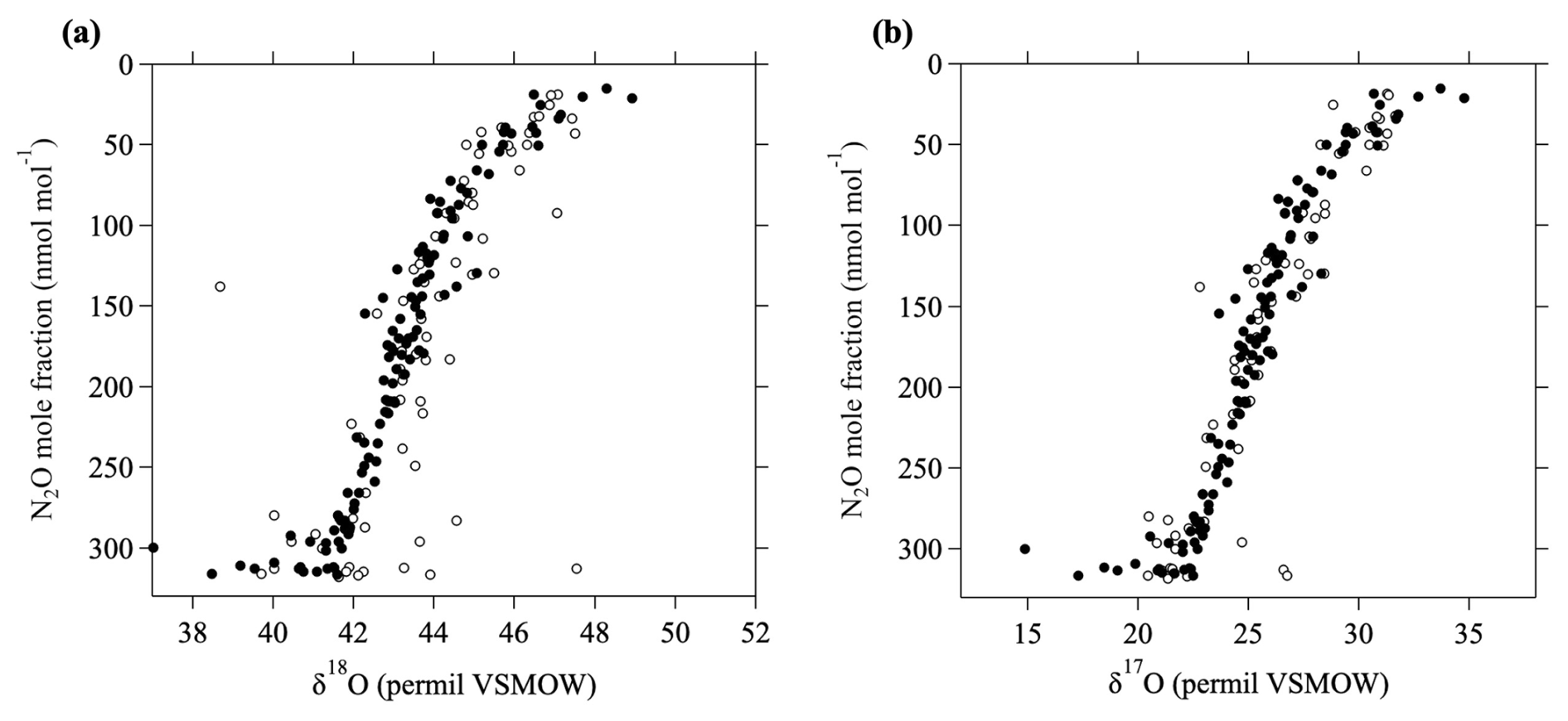
Figure 1 The relationship between the N₂O mole fraction and (a) δ¹⁸O in CO₂ and (b) δ¹⁷O in CO₂. δ¹⁸O and δ¹⁷O values measured by Kawagucci et al. (2008) are shown by open circles. δ¹⁸O and δ¹⁷O values calculated assuming an MIE factor of 1.7 (see text) in this study are shown by closed circles.

While cryogenically extracting CO₂ from the air sample, N₂O was simultaneously trapped with the CO₂. Because N₂O and CO₂ have the same mass number, we must correct for N₂O to obtain the true δ¹³C value. The correction method was described in detail by Nakazawa et al. (1993), and we summarize it here. The ionization efficiency of N₂O was measured in advance, and the measured δ¹³C value was corrected using the ${\mathrm{N}}_{\mathrm{2}}\mathrm{O}/{\mathrm{CO}}_{\mathrm{2}}$ mole fraction ratio of the air sample. In the troposphere, the ${\mathrm{N}}_{\mathrm{2}}\mathrm{O}/{\mathrm{CO}}_{\mathrm{2}}$ mole fraction ratio does not change significantly, and the N₂O correction is almost constant (approximately +0.2 ‰; Nakazawa et al., 1997a). However, because the N₂O mole fraction decreases rapidly with increasing altitude in the stratosphere (e.g., Toyoda et al., 2001), the ${\mathrm{N}}_{\mathrm{2}}\mathrm{O}/{\mathrm{CO}}_{\mathrm{2}}$ mole fraction ratio decreases with altitude, and the magnitude of the N₂O correction also varies vertically. Therefore, the N₂O correction also strongly influences the observed vertical distribution of δ¹³C in the stratosphere.

Stratospheric air samples were also measured for δ¹³CH₄ using a gas chromatograph-combustion-isotope ratio spectrometer developed at the National Institute of Polar Research (NIPR), Japan. The method has been described in detail by Morimoto et al. (2006) and is briefly summarized here. An air sample was flushed by pure helium and passed through a trap containing HayeSep D at a temperature of −120 °C to concentrate CH₄ in the sample. Then, the CH₄ was released and transferred into a PoraBOND Q cryofocusing trap at −197 °C. The CH₄ released from the trap when brought to room temperature was separated from the residual components using a PoraPLOT Q capillary column and combusted into CO₂ in a furnace with a Pt-Ni-Cu catalyst at 940 °C. The converted CO₂ was analyzed using a continuous-flow mass spectrometer (Finnigan MAT252). The precision was reported to be 0.06 ‰ (Morimoto et al., 2006). Before 1996, δ¹³CH₄ measurements were performed using off-line oxidation equipment (Sugawara et al., 1997), in which CH₄ in the sample was converted to CO₂ using a catalyst (0.5  % Pt supported on alumina pellets) at 750 °C, and the pure CO₂ sample thus prepared was analyzed using the mass spectrometer installed at TU in the same way as for δ¹³CO₂, except using a micro-volume inlet system. The overall analytical precision was 0.07 ‰ (Sugawara et al., 1997). To produce a high-quality data record, we needed to verify that these two methods produced the same results. Therefore, several sets of stratospheric air samples were analyzed using both methods, and the δ¹³CH₄ results differed by about 0.85 ‰. To correct for this difference, the off-line measurement results were adjusted to match the on-line measurements. In this study, the δ¹³CH₄ value is reported relative to VPDB. The international comparison of δ¹³CH₄ measurements described in detail by Umezawa et al. (2018) revealed a difference of 0.2 ‰ between NIPR and the Institute of Arctic and Alpine Research (INSTAAR) results. Therefore, all δ¹³CH₄ values observed by the National Oceanic and Atmospheric Administration Global Monitoring Laboratory (NOAA/GML) and INSTAAR were shifted to match the NIPR scale.

The method used to analyze GS is described in Appendix A.

3 Results and discussion

3.1 Vertical profiles of CO₂ mole fraction and δ¹³CO₂

Figure 2 shows vertical profiles of the CO₂ mole fraction and δ¹³CO₂ over Japan throughout the study period. CO₂ mole fractions and δ¹³CO₂ values have increased and decreased, respectively, from 1985 to 2020. Vertical δ¹³CO₂ profiles observed by Gamo et al. (1995) in 1985 and 1986 are included in this figure after MIE correction. Previous studies reported that the CO₂ mole fraction decreases with increasing altitude from the tropopause to around 20–25 km, and then it becomes almost constant at higher altitudes (Nakazawa et al., 1995, 2002). Our CO₂ mole fraction data show a similar vertical distribution during the observation period. Because our δ¹³CO₂ data are more scattered with respect to altitude than the CO₂ mole fraction, we calculated detrended vertical δ¹³CO₂ profiles as follows. First, the long-term trend of the tropospheric δ¹³CO₂ at Mauna Loa, Hawaii (hereafter, MLO) (Michel et al., 2025) was calculated as a representative tropospheric trend, and all our stratospheric δ¹³CO₂ observation data were shifted up or down based on that trend to produce values corresponding to August 2016 for comparison with the model results described below. Then, the δ¹³CO₂ values thus obtained for the entire study period were grouped into 11 2 km vertical bins, and the average value for each bin was calculated (Fig. 2c). The results showed that δ¹³CO₂ values increased with increasing altitude from near the tropopause to around 25 km and then decreased slightly above that altitude. Gamo et al. (1989) originally reported that δ¹³CO₂ values increased by approximately 0.4 ‰ from the tropopause to 25 km altitude in September 1985, whereas our recalculated results showed an increase of about 0.2 ‰ (Fig. 2b). The average increase shown in Fig. 2c was even smaller, only about 0.1 ‰. This difference between the vertical profiles originally reported by Gamo et al. (1989) and our present results is due to our incorporation of the MIE on ¹⁷O and ¹⁸O (Sect. 2.2).

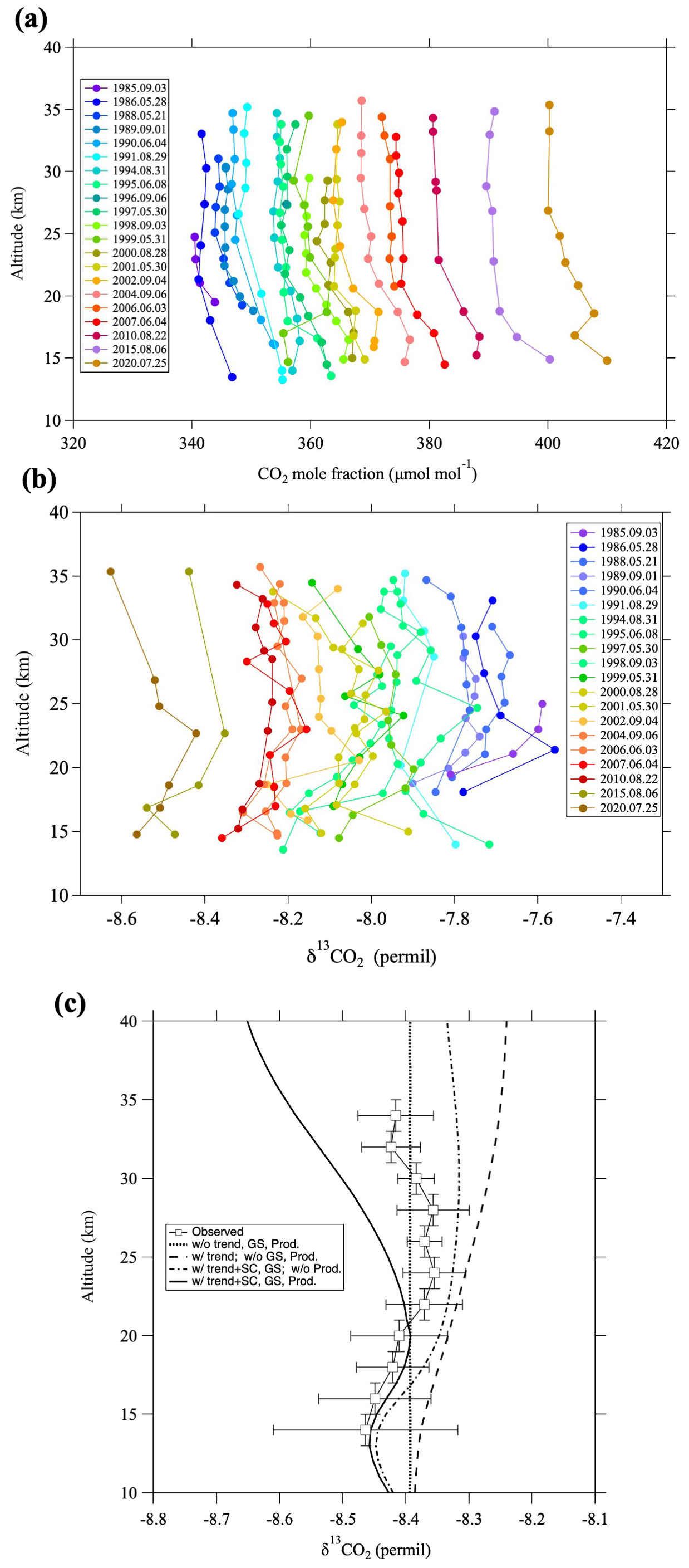
Figure 2 Vertical profiles of (a) CO₂ mole fraction and (b) δ¹³CO₂ over Japan during the period 1985–2020. (c) δ¹³CO₂ values averaged over the study period and grouped in 11 2 km vertical bins (open squares). Curves show 2-D modeling results without the tropospheric trend, seasonal cycle, gravitational separation (GS), or airborne sources (thick dotted line), including only the tropospheric trend (dashed line), including the tropospheric trend, seasonal cycle, and GS (dotted-dashed line), and including the tropospheric trend, seasonal cycle, GS, and airborne sources (solid line).

Below an altitude of ∼ 17 km, δ¹³CO₂ values are quite variable, often being irregularly high or low depending on the observation year, which is exhibited by the large error bars in Fig. 2c. Based on detailed aircraft observations of δ¹³CO₂ variations in the troposphere over Japan, Nakazawa et al. (1993) reported that the seasonal cycle of δ¹³CO₂ between 8 km altitude and the tropopause show a minimum around May and a maximum around September, with a peak-to-peak amplitude of 0.36 ‰. Indeed, our balloon observations were conducted in either spring (late May to early June) or summer (late July to early September), and the observed δ¹³CO₂ values at lower altitudes tended to be lower in spring and higher in summer. Accordingly, we attribute the large δ¹³CO₂ variations below an altitude of 17 km to the upper tropospheric air itself, or stratospheric air directly influenced by the troposphere.

Our data clearly reveal a secular decrease in mid-stratospheric δ¹³CO₂ values. To compare the temporal variations of δ¹³CO₂ in the mid-stratosphere with those in the troposphere, the δ¹³CO₂ values obtained by averaging mid-stratospheric data above 24 km altitude (30 hPa) from each year and monthly average MLO data are shown in Fig. 3. When comparing our data with the NOAA/GML and INSTAAR data at MLO (Michel et al., 2025), any possible offset of δ¹³CO₂ measurements should be taken into account. The inter-comparison results of the WMO/IAEA Round Robin Comparison Experiment (https://gml.noaa.gov/ccgg/wmorr/, last access: 20 February 2025) show that our values are approximately 0.07 ‰ lower than INSTAAR values. In this study, we directly compared δ¹³CO₂ data at Ny-Ålesund, Svalbard observed by Goto et al. (2017) with the INSTAAR data at the Zeppelin Observatory (ZEP) in Ny-Ålesund because we used the same δ¹³CO₂ measurement system and standard scale as Goto et al. (2017). Monthly average δ¹³CO₂ values at Ny-Ålesund from both studies were calculated by applying a curve-fitting procedure (Nakazawa et al., 1997b) over the years compared, 1996–2014. As a result, we estimated the difference between this study and INSTAAR data to be insignificant (−0.005 ± 0.067 ‰) and did not apply any further correction to our δ¹³CO₂ data. The average rate of change of δ¹³CO₂ in the mid-stratosphere was calculated to be −0.026 ± 0.001 ‰ yr⁻¹ for the period 1985–2020, consistent with the average rate of change at MLO from 1990 to 2024 (−0.026 ± 0.001 ‰ yr⁻¹) despite the slightly different time periods. Tropospheric δ¹³CO₂ values are known to decrease over time due to the emission of CO₂ with low δ¹³CO₂ by anthropogenic fossil fuel consumption, and our results show that a similar decreasing trend is observable in the stratosphere. It is also well known that mid-stratospheric air over the mid-latitudes is “aged,” mainly because of the slow transport of air from the tropical tropopause to the mid-latitude mid-stratosphere. Indeed, the age of mid-stratospheric air estimated from CO₂ mole fractions was approximately 4.4 yr older on average than that of tropical tropospheric air (see Sect. 3.5). Nevertheless, the δ¹³CO₂ values observed in the mid-stratosphere over Japan did not seem to show any significant time delay compared with the observed values in the tropical troposphere. Although systematic observations of δ¹³CO₂ have not yet been performed in the tropical upper troposphere where stratospheric air originates, Assonov et al. (2010) found from CARIBIC aircraft observations that δ¹³CO₂ variations in the tropical upper troposphere are close to those at MLO. Therefore, if we assume no difference between the δ¹³CO₂ values at MLO and those in the tropical upper troposphere, the lack of a delay between the values in the mid-stratosphere over Japan and those at MLO clearly contradicts the concept of the age of air. Simply following the logic of the age of air, we would expect the decrease of stratospheric δ¹³CO₂ to lag behind the tropospheric trend, such that the δ¹³CO₂ value at any given time should be higher in the mid-stratosphere than in the troposphere. This discrepancy suggests that δ¹³CO₂ is not a conserved quantity in the stratosphere and is instead modified not only by air transport but also by other mechanisms. In the following sections we discuss possible mechanisms in detail.

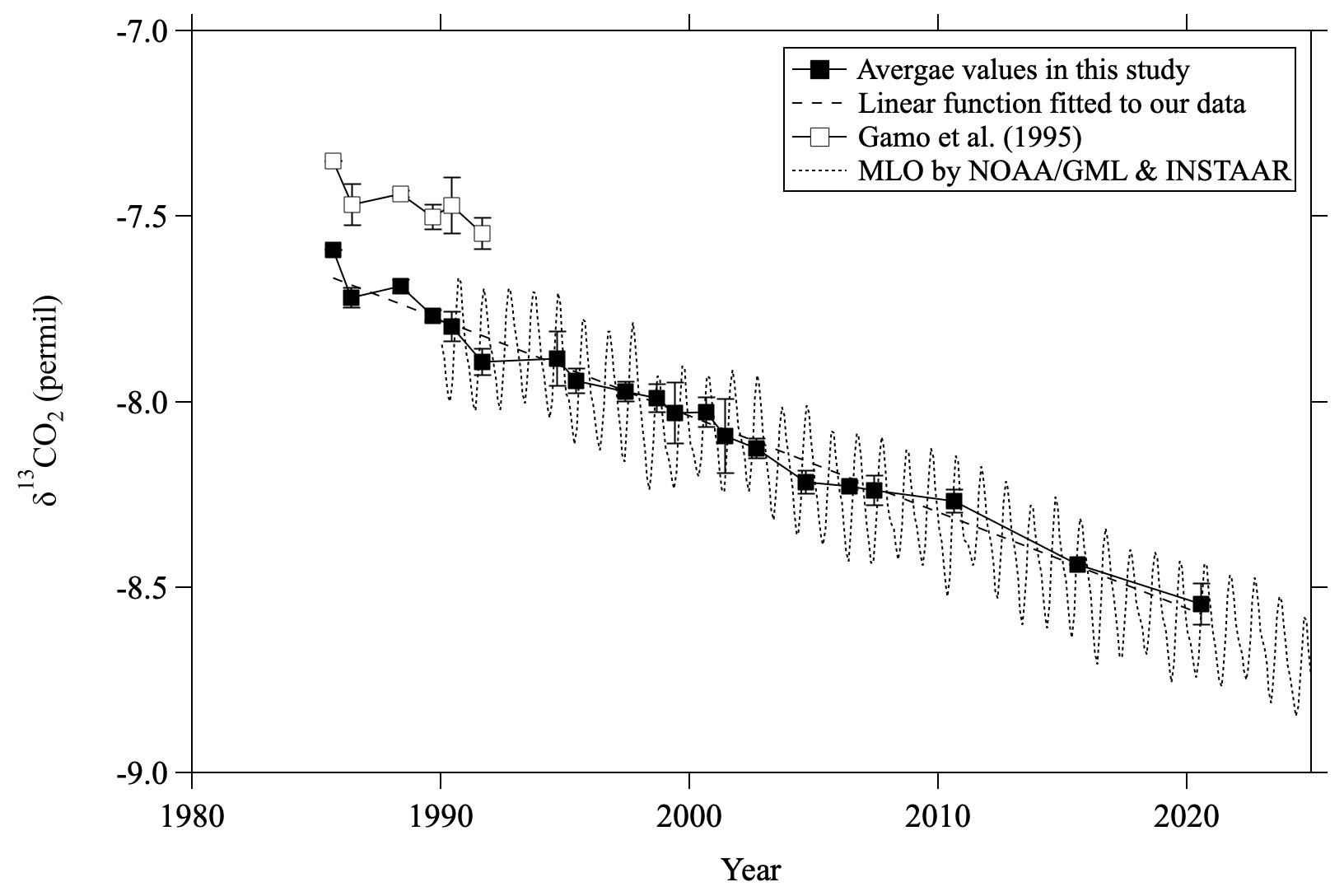
Figure 3 Average mid-stratospheric (>24 km altitude) δ¹³CO₂ values over Japan (closed squares). The linear function fitted to the average values using the least-squares method is shown by the dashed line. Values reported by Gamo et al. (1995) are shown by open squares. Monthly average δ¹³CO₂ observed at Mauna Loa by NOAA/GML and INSTAAR (Michel et al., 2025) is also shown by the dotted line.

3.2 Airborne CO₂ source from CH₄ oxidation

In the stratosphere, CH₄ is destroyed by reactions with OH, O(¹D), and Cl, which produce intermediate products such as CH₃O₂ and CH₂O. These products are immediately converted to CO because of their short lifetimes. However, CO is also destroyed by reaction with OH. Therefore, the chemical budget of CO in the stratosphere is expressed as (Minschwaner et al., 2010)

$$\begin{array}{}\text{(4)}& \begin{array}{rl}{\displaystyle \frac{d\left[\mathrm{CO}\right]}{\mathrm{d}t}}& =\left[{\mathrm{CH}}_{\mathrm{4}}\right](k_{{\mathrm{CH}}_{\mathrm{4}}+\mathrm{OH}}\left[\mathrm{OH}\right]\\ & +k_{{\mathrm{CH}}_{\mathrm{4}}+\mathrm{Cl}}\left[\mathrm{Cl}\right]+k_{{\mathrm{CH}}_{\mathrm{4}}+\mathrm{O}}\left[\mathrm{O}{(}^{\mathrm{1}}\mathrm{D}\right)\left]\right)\\ & +J_{{\mathrm{CO}}_{\mathrm{2}}}\left[{\mathrm{CO}}_{\mathrm{2}}\right]-k_{\mathrm{CO}+\mathrm{OH}}\left[\mathrm{CO}\right]\left[\mathrm{OH}\right],\end{array}\end{array}$$

where $k_{{\mathrm{CH}}_{\mathrm{4}}+\mathrm{OH}}$, $k_{{\mathrm{CH}}_{\mathrm{4}}+\mathrm{Cl}}$, $k_{{\mathrm{CH}}_{\mathrm{4}}+\mathrm{O}}$, and k_CO+OH are the reaction rates for the respective chemical reactions, and $J_{{\mathrm{CO}}_{\mathrm{2}}}$ is the rate of photodissociation of CO₂. The last term on the right-hand side of this equation represents the oxidation of CO to CO₂. Although the amount of CO₂ produced this way is small compared to the stratospheric abundance, it cannot be ignored as an airborne source, especially in terms of isotopic signatures. The timescales for the photochemical loss and production of CO in the mid-latitude mid-stratosphere (∼ 35 km altitude) are about 30 d (Minschwaner et al., 2010), quite short compared to the timescale of the stratospheric mean meridional circulation (more than several years). If we assume that the chemical budget of CO is in a steady state and that CO₂ photodissociation is negligibly small below the mid-stratosphere, the rate of CH₄ loss should equal the rate of CO₂ production. Indeed, to estimate the age of stratospheric air from the CO₂ mole fraction, a small amount of CO₂ produced by the chemical destruction of CH₄ was taken into account (e.g., Engel et al., 2002; Sugawara et al., 2018). To correct for this effect, each observed CO₂ mole fraction was adjusted using the CH₄ mole fraction measured from the corresponding air sample prior to age calculation (see Appendix C). The adjustment increases with increasing altitude and becomes larger than 1 µmol mol⁻¹ at the highest altitudes. As with the CO₂ mole fraction, ¹³C can be corrected by assuming a steady-state ¹³CO budget in which ¹³C is added to ¹³CO₂ from ¹³CH₄ through a series of oxidation reactions from CH₄ to CO₂. Indeed, it is well known that isotopic fractionation occurs during CH₄ oxidation (Saueressig et al., 1995; Sugawara et al., 1997; Rice et al., 2003; Röckmann et al., 2011).

Figure 4a, b shows the vertical CH₄ mole fraction and δ¹³CH₄ profiles observed over Japan, respectively. A common feature of both profiles is their rapid change with altitude, although δ¹³CH₄ values increase, whereas the mole fractions decrease with increasing altitude. Such vertical distributions have been attributed to large kinetic isotopic effects (KIEs) associated with the chemical destruction of CH₄ in the stratosphere (Sugawara et al., 1997; Rice et al., 2003; Röckmann et al., 2011). KIEs on CH₄ have also been studied using numerical models (Saueressig et al., 2001; Wang et al., 2002; McCarthy et al., 2003). In previous studies, the apparent fractionation factor was derived from the Rayleigh distillation model by assuming that the chemical destruction of CH₄ occurs in a closed system (Sugawara et al., 1997; Rice et al., 2003). In general, the Rayleigh distillation model for the CH₄ mole fraction and δ¹³CH₄ is expressed as

$$\begin{array}{}\text{(5)}& {\mathit{\delta }}^{\mathrm{13}}{\mathrm{CH}}_{\mathrm{4}}=\left({\mathit{\delta }}^{\mathrm{13}}{\mathrm{CH}}_{\mathrm{4}\mathrm{\_}\mathrm{0}}+\mathrm{1}\right){\mathit{\mu }}^{\mathit{\alpha }-\mathrm{1}}-\mathrm{1},\end{array}$$

where δ¹³CH_{4_0}, µ, and α are the isotopic ratio before CH₄ is destroyed, the ratio of mole fractions (μ=$\left[{\mathrm{CH}}_{\mathrm{4}}\right]/[{\mathrm{CH}}_{\mathrm{4}}{]}_{\mathrm{0}}$), and the apparent fractionation factor, respectively. The apparent fractionation factor can be estimated by applying Eq. (5) to observed data. We note that [CH₄]₀ and δ¹³CH_{4_0} change with time and should be taken here as the values in the tropical upper troposphere at the time when air entered the stratosphere through the tropical tropopause layer (TTL). Therefore, the tropical upper tropospheric records of CH₄ and δ¹³CH₄ were used to give [CH₄]₀ and δ¹³CH_{4_0} values going back in time based on the mean age estimated from CO₂ mole fractions (see Appendix C). Details of the tropical upper tropospheric records of CH₄ and δ¹³CH₄ are described in Sect. 3.5. Figure 4c shows that the relationship between ln {(δ¹³CH${}_{\mathrm{4}}+\mathrm{1})/({\mathit{\delta }}^{\mathrm{13}}$CH_{4_0}+1)} and ln([CH₄] $/$ [CH₄]₀) can be approximated by linear functions if we divided the data between the lower (<24 km) and mid-stratosphere (>24 km), with the upper layer showing larger isotopic fractionation effects. The apparent fractionation factors calculated using the least-squares method were 0.9889 ± 0.0003 and 0.9866 ± 0.0007 for the lower and mid-stratosphere, respectively. We attributed these differences in apparent fractionation factors to differences in the relative contributions of the CH₄ reactions with OH, O(¹D), or Cl over the air transport pathway, and/or the effect of air mixing (Röckmann et al., 2011).

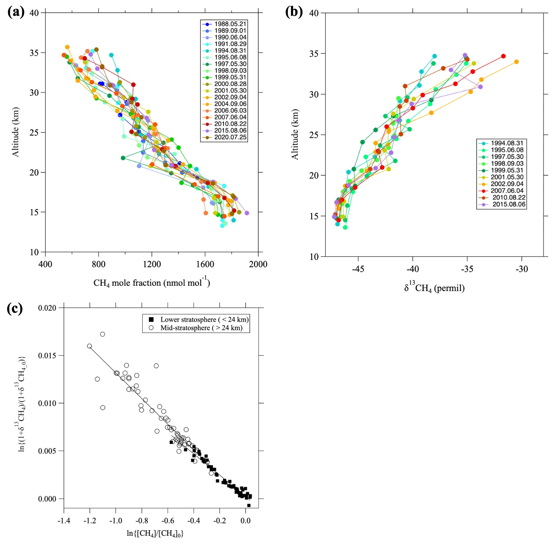
Figure 4 Vertical profiles of (a) CH₄ mole fraction and (b) δ¹³CH₄ over Japan, and (c) the relationship between ln{(δ¹³CH${}_{\mathrm{4}}+\mathrm{1})/({\mathit{\delta }}^{\mathrm{13}}$CH_{4_0}+1)} and ln([CH₄] $/$ [CH₄]₀). In (c), the data are divided into the lower (<24 km, closed squares) and mid-stratosphere (>24 km, open circles), and the linear functions fitted to each dataset using the least-squares method are shown by lines.

Equation (5) expresses the relationship between the mole fraction and isotopic ratio of the remaining CH₄. Similarly, focusing on the CH₄ lost via the CH₄–CO–CO₂ chain reaction, the relationship between the CH₄ mole fraction and isotopic ratio of lost CH₄ (hereafter, δ¹³CH_{4_L}) is derived from Eq. (5) as

$$\begin{array}{}\text{(6)}& {\mathit{\delta }}^{\mathrm{13}}{\mathrm{CH}}_{\mathrm{4}\mathrm{\_}\mathrm{L}}=\left({\mathit{\delta }}^{\mathrm{13}}{\mathrm{CH}}_{\mathrm{4}\mathrm{\_}\mathrm{0}}+\mathrm{1}\right){{\displaystyle \frac{\mathrm{1}-\mathit{\mu }}{\mathrm{1}-\mathit{\mu }}}}^{\mathit{\alpha }}-\mathrm{1}.\end{array}$$

Here, the removed CH₄ includes the total amount of CH₄ loss integrated over the air transport pathway. Based on this equation, we calculated δ¹³CH_{4_L} for each year's data from the observed CH₄ mole fractions and apparent fractionation factors by grouping them into altitudes below and above 24 km. Typical δ¹³CH_{4_L} values were about −57 ‰, −56 ‰, and −55 ‰ around altitudes of 20, 30, and 35 km, respectively. The stratospheric δ¹³CO₂ values were corrected for airborne sources simply by assuming that carbon with the isotopic ratio of δ¹³CH_{4_L} was added to ambient CO₂. We note that the amount of CO₂ added by CH₄ oxidation was estimated from the difference between the CH₄ mole fraction observed in the mid-latitude stratosphere and that estimated at the tropical upper troposphere; this does not represent chemical production at the observed location, but apparent production, because CH₄ oxidation occurs along the transport pathway of the air mass and is accompanied by air mixing. Consequently, the depression of CH₄ integrated over the air transport pathway is observed at a certain location in the stratosphere. Because we assumed the simple Rayleigh distillation model, the δ¹³CH_{4_L} estimated here is also an apparent value in a similar sense as described above. Accordingly, our assumption described above was a first-order approximation to correct δ¹³CO₂ for airborne CO₂ sources.

As an example, we corrected the vertical distributions of the CO₂ mole fraction and δ¹³CO₂ (Fig. 5a) and compared with the CH₄ mole fraction and δ¹³CH₄ (Fig. 5b) observed on 22 August 2010. The results indicated that the δ¹³CO₂ value decreased by 0.14 ‰ and the CO₂ mole fraction increased by approximately 1.1 µmol mol⁻¹ at the highest altitude (∼ 34 km) when corrected for airborne CO₂ sources. Therefore, such a correction for the airborne CO₂ source with low δ¹³CO₂ values produced by CH₄ oxidation is essential for understanding CO₂ mole fraction and δ¹³CO₂ variations in the mid-stratosphere. This effect is particularly strong on δ¹³CO₂ and significantly impacted the shape of the vertical distribution.

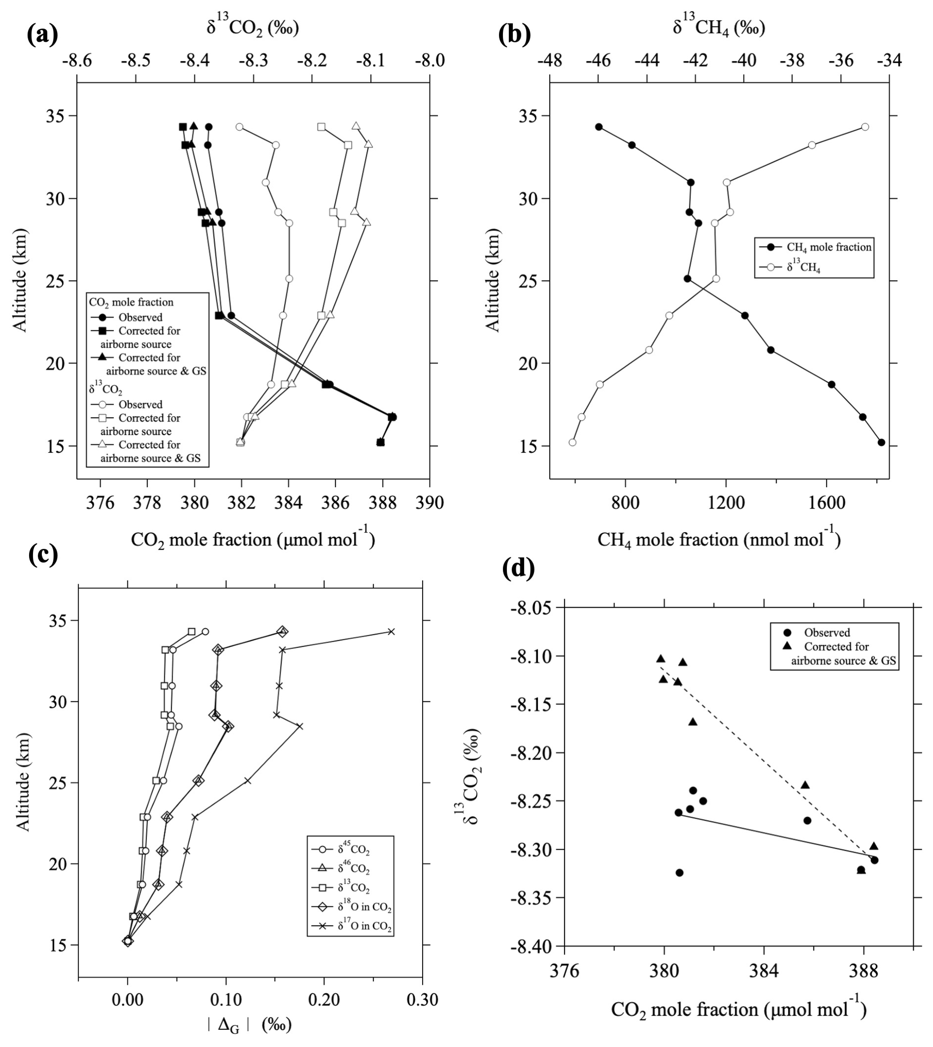
Figure 5 (a) Vertical profiles of the CO₂ mole fraction (closed circles) and δ¹³CO₂ (open circles) observed over Japan on 22 August 2010. Values corrected for airborne CO₂ sources (squares) and additionally for gravitational separation (GS; triangles) are also shown. (b) Vertical profiles of the CH₄ mole fraction (closed circles) and δ¹³CH₄ (open circles). (c) Vertical profiles of the magnitude of GS corrections, $\left|{\mathrm{\Delta }}_{\mathrm{G}}\right|$, for δ⁴⁵CO₂ (circles), δ⁴⁶CO₂ (triangles), δ¹³CO₂ (squares), δ¹⁸O (diamonds), and δ¹⁷O (crosses) in CO₂. (d) Observed δ¹³CO₂ plotted against CO₂ mole fraction (closed circles) and those corrected for airborne CO₂ sources and GS (triangles). Lines are linear functions fitted to each trend by the least-squares method.

We note that the transport of CO from the troposphere into the stratosphere and its oxidation in the lower stratosphere are not considered in the above discussion. Because the photochemical timescales of CO are longer in the lower stratosphere than in the mid-stratosphere, tropospheric CO could be a stratospheric CO₂ source associated with troposphere–stratosphere exchange and may be important in the lower stratospheric CO budget. Observational results on the stable carbon isotopic ratio of CO, δ¹³CO, have been reported not only for the troposphere (Brenninkmeijer, 1993; Röckmann and Brenninkmeijer, 1997; Röckmann et al., 1999, 2002; Kato et al., 2000) but also for the lower stratosphere (Brenninkmeijer et al., 1996; Röckmann et al., 2024). In particular, Brenninkmeijer et al. (1996) found that extremely low δ¹³CO values in the southern high-latitude lower stratosphere are accompanied by increasing δ¹³CH₄ values and suggested that the large KIE of CH₄ destruction by Cl plays an important role. The local production of CO by CH₄-destruction-depleted ¹³C in stratospheric CO is consistent with the above discussion if CO is rapidly oxidized to CO₂ depleted in ¹³C. However, tropospheric CO could be an additional airborne CO₂ source if it is transported into the lower stratosphere and oxidized to CO₂. Previous studies have reported that δ¹³CO values in the free troposphere are around −30 ‰ to −25 ‰ (Brenninkmeijer, 1993; Röckmann and Brenninkmeijer, 1997; Röckmann et al., 1999, 2002; Kato et al., 2000), and the KIE on carbon in the reaction CO + OH depends on atmospheric pressure (Stevens and Wagner, 1989; Bergamaschi et al., 2000). Its fractionation factor is 0.994 (expressed as the ratio of rate constants, ${}^{\mathrm{13}}k{/}^{\mathrm{12}}k)$ at 1013 hPa, but increases to about 1.000 at 400 hPa and further to 1.003–1.005 above the tropopause. Therefore, CO₂ produced from the reaction CO + OH should be slightly enriched in ¹³C in the stratosphere, contrary to CO₂ produced in the lower troposphere. Accordingly, tropospheric CO could be an airborne CO₂ source with δ¹³C values lower than around −25 ‰ to −20 ‰ in the lower stratosphere. Assuming that tropospheric air containing 250 nmol mol⁻¹ CO with δ¹³CO $=-$30 ‰ is transported to the stratosphere where 200 nmol mol⁻¹ CO is lost by reaction with OH, δ¹³CO₂ values should decrease by only about 0.01 ‰ when 0.2 µmol mol⁻¹ CO₂ with δ¹³CO${}_{\mathrm{2}}=-\mathrm{28}$ ‰ is added to 390 µmol mol⁻¹ CO₂ with δ¹³CO${}_{\mathrm{2}}=-\mathrm{8.5}$ ‰. Therefore, this effect would be negligibly small compared with the influence of CH₄ oxidation. Unfortunately, we could not further evaluate the effect of tropospheric CO from our observations, and further study including measurements of δ¹³CO is needed.

3.3 Gravitational separation of δ¹³CO₂

The standardized GS is defined as 〈δ_G〉, which is normalized by the mass number differences of corresponding molecules (see Appendix A). With respect to δ¹³CO₂, the upward decrease due to GS is equal to 〈δ_G〉 for ¹³C¹⁶O₂ and ¹²C¹⁷O¹⁶O (Δm=1), and is twice as large for ¹²C¹⁸O¹⁶O, ¹³C¹⁷O¹⁶O, and ¹²C¹⁷O₂ (Δm=2). Therefore, GS equal to and twice the magnitude of 〈δ_G〉 can be considered to act on δ⁴⁵CO₂ and δ⁴⁶CO₂, respectively:

$$\begin{array}{}\text{(7a)}& {\mathrm{\Delta }}_{\mathrm{G}}\left({\mathit{\delta }}^{\mathrm{45}}{\mathrm{CO}}_{\mathrm{2}}\right)=\langle {\mathit{\delta }}_{\mathrm{G}}\rangle -\langle {\mathit{\delta }}_{\mathrm{G}}{\rangle }_{\mathrm{0}},\end{array}$$

$$\begin{array}{}\text{(7b)}& {\mathrm{\Delta }}_{\mathrm{G}}\left({\mathit{\delta }}^{\mathrm{46}}{\mathrm{CO}}_{\mathrm{2}}\right)=\mathrm{2}\left(\langle {\mathit{\delta }}_{\mathrm{G}}\rangle -\langle {\mathit{\delta }}_{\mathrm{G}}{\rangle }_{\mathrm{0}}\right).\end{array}$$

Here, Δ_G(x) and 〈δ_G〉₀ represent the change in isotopic value x due to GS and the value of 〈δ_G〉 before GS occurs (i.e., corresponding to the relevant value in the upper troposphere), respectively. Because 〈δ_G〉−〈δ_G〉₀ is negative in the stratosphere (see Appendix A), Δ_G(δ⁴⁵CO₂) and Δ_G(δ⁴⁶CO₂) are also negative. When δ¹³CO₂ was corrected for GS, Eqs. (7a) and (7b) were first applied to δ⁴⁵CO₂ and δ⁴⁶CO₂, respectively, and then δ¹³CO₂ was determined using the MIE algorithm described in Sect. 2.2. As shown in Fig. 5c, |Δ_G(δ¹³CO₂)| was slightly smaller than (about 82 % of) |Δ_G(δ⁴⁵CO₂)| in the mid-stratosphere, mainly because of ¹²C¹⁷O¹⁶O enrichment due to the MIE in the stratosphere.

The same method can be applied to the mole fraction of a specific molecule (Ishidoya et al., 2006):

$$\begin{array}{}\text{(8)}& {\mathrm{\Delta }}_{\mathrm{G}}\left(C\right)=C_{\mathrm{0}}\times \left(m-m_{\mathrm{air}}\right)\times \left(\langle {\mathit{\delta }}_{\mathrm{G}}\rangle -\langle {\mathit{\delta }}_{\mathrm{G}}{\rangle }_{\mathrm{0}}\right).\end{array}$$

Here, C₀ and C denote the mole fractions of the molecule before and after GS, respectively, and m and m_air are the respective mass numbers of the molecule and air. The maximum depression of the CO₂ mole fraction amounts to about 0.6 µmol mol⁻¹ at the highest altitude, assuming C₀=400 µmol mol⁻¹ and $\langle {\mathit{\delta }}_{\mathrm{G}}\rangle -\langle {\mathit{\delta }}_{\mathrm{G}}{\rangle }_{\mathrm{0}}=-\mathrm{100}$ per meg (10⁻⁶). As an example, the vertical profile of the CO₂ mole fraction obtained by correcting the 22 August 2010 observations for GS is shown in Fig. 5a. Compared to the profiles corrected for airborne CO₂ sources, GS correction increases the CO₂ mole fraction by 0.4 µmol mol⁻¹ and the δ¹³CO₂ by approximately 0.06 ‰ at 34 km altitude. Although the effect of GS on the CO₂ mole fraction is small, that on δ¹³CO₂ is non-negligible, significantly influencing the vertical profile along with CH₄ oxidation. In this regard, the mean age estimated from the CO₂ mole fraction without GS correction has an older age bias that increases with increasing altitude. The age bias is negligibly small (<1 month) in the lower stratosphere but not negligible in the mid-stratosphere (>2 months at 35 km altitude). Therefore, we applied the GS correction to the CO₂ mole fraction to estimate the CO₂ age, as described in Appendix C.

Correcting for both CH₄ oxidation and GS, δ¹³CO₂ values increase with altitude and become nearly constant above ∼ 25 km; they are clearly anticorrelated with the CO₂ mole fraction. Assuming a linear relationship between the CO₂ mole fraction and δ¹³CO₂ (Fig. 5d), the slope calculated by least squares is −0.005 ± 0.003 ‰ (µmol mol${}^{-\mathrm{1}}{)}^{-\mathrm{1}}$ for the raw observational data and −0.023 ± 0.002 ‰ (µmol mol${}^{-\mathrm{1}}{)}^{-\mathrm{1}}$ for the corrected data. This rate of change for the corrected data is less negative than approximately −0.05 ‰ (µmol mol${}^{-\mathrm{1}}{)}^{-\mathrm{1}}$ for the seasonal cycles in the troposphere (Nakazawa et al., 1993) and is near the rate of change for their secular trends (Morimoto et al., 2000; Goto et al., 2017). Generally, because of the Brewer–Dobson circulation, air at higher altitudes is older. Therefore, we consider that this rate of change for the corrected data basically reflects different ages of air.

3.4 Two-dimensional model of stratospheric δ¹³CO₂

The mechanisms governing the vertical δ¹³CO₂ profile in the stratosphere are shown schematically in Fig. 6, including the influence of the age of air as well as the effects of CH₄ oxidation and GS discussed in Sects. 3.2 and 3.3. Tropospheric δ¹³CO₂ values have been decreasing through time due to the combustion of fossil fuels. If it is assumed that ¹²CO₂ and ¹³CO₂ have no sinks or sources in the stratosphere, the air that intrudes from the tropical upper troposphere is slowly transported to the mid-latitude stratosphere by the Brewer–Dobson circulation, conserving the δ¹³CO₂ value. Therefore, based on the concept of age of air, it is expected that δ¹³CO₂ values should also decrease with time in the stratosphere after a certain lag time. Accordingly, δ¹³CO₂ values should be higher in the mid-stratosphere than in the troposphere (dotted line in Fig. 6). In contrast, GS decreases δ¹³CO₂ values at higher altitudes because ¹³C¹⁶O₂ is heavier than ¹²C¹⁶O₂ (dashed line in Fig. 6). In addition, ¹³C-depleted CO₂ produced by CH₄ oxidation further decreases δ¹³CO₂ values at high altitudes (solid line in Fig. 6). The observed stratospheric vertical δ¹³CO₂ profile should therefore be formed by a combination of these effects.

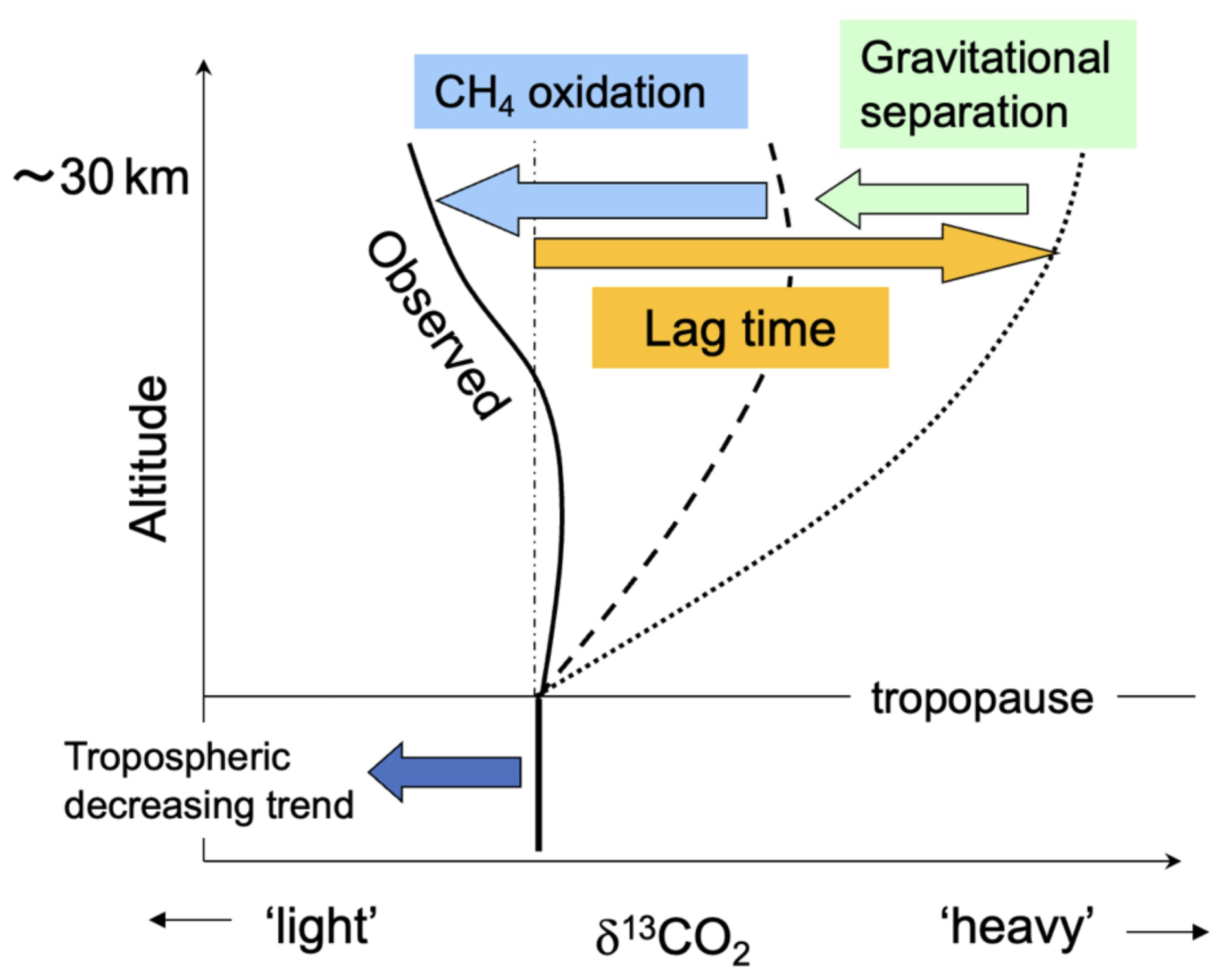
Figure 6 Schematic representation of the mechanisms influencing the vertical profile of stratospheric δ¹³CO₂ (see text).

To verify this hypothesis, we performed numerical simulations using a two-dimensional model of the middle atmosphere (SOCRATES) developed by the National Center for Atmospheric Research (NCAR; Huang et al., 1998; Park et al., 1999; Khosravi et al., 2002). Details of the model calculations are described in Appendix B. The monthly average meridional δ¹³CO₂ distribution calculated by SOCRATES for August 2016, which includes the effects of CH₄ oxidation and GS, is shown in Fig. 7. The effect of the CO₂ production associated with the KIE on CH₄ destruction is included in a simplified manner (see Appendix B). The δ¹³CO₂ values decrease with increasing altitude up to about 14 km and then increase up to about 20 km in the mid-latitudes of the northern hemisphere during summer. The distribution of δ¹³CO₂ from the troposphere to the lower stratosphere should therefore be closely related to the propagation of its seasonal cycle in the troposphere. δ¹³CO₂ values reach a maximum at around 20 km and then gradually decrease. At high latitudes in the southern (winter) hemisphere, the vertical decrease of δ¹³CO₂ is significant, suggesting that the effects of CH₄ oxidation and GS are enhanced by the descending upper atmosphere.

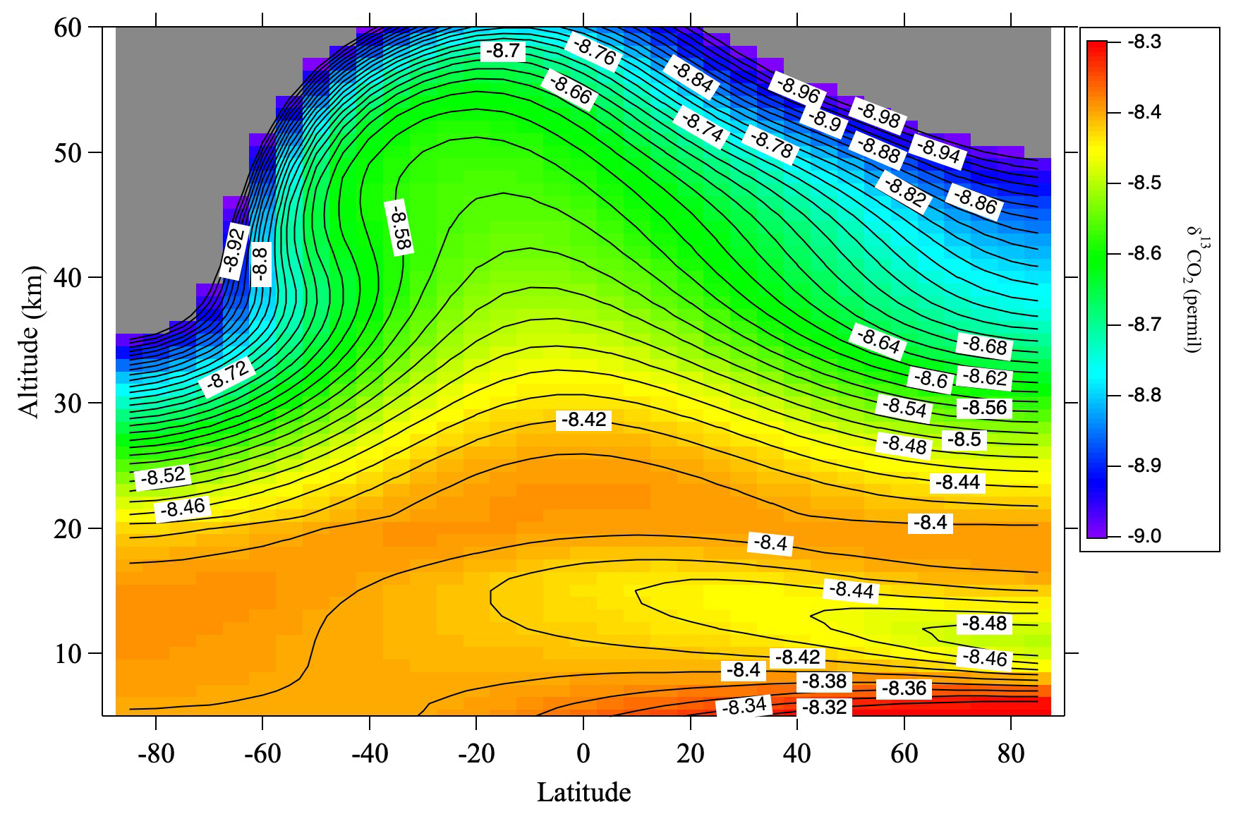
Figure 7 Monthly average meridional distribution of δ¹³CO₂ for August 2016 calculated using the SOCRATES model. Values lower than −9.0 ‰ are colored gray.

To investigate the vertical δ¹³CO₂ profile in detail, we compared this model with our observations in Fig. 2c. The modeled δ¹³CO₂ profile calculated without accounting for CH₄ oxidation and GS increased with increasing altitude, and it was 0.14 ‰ higher at altitudes around 35 km than near the tropopause. Because the average rate of change of the long-term δ¹³CO₂ record at MLO is −0.026 ‰ yr⁻¹ for the period 1990–2022, the lag time at 35 km (0.14 ‰ divided by 0.026 ‰ yr⁻¹) should be approximately 5.4 yr, nearly consistent with the calculated mean age of air (see Appendix C). If the effect of GS is further taken into account, the δ¹³CO₂ decreased by approximately 0.07 ‰ at 35 km. The most significant impact on the modeled vertical profile was the effect of CH₄ oxidation, which imparted a decrease of 0.26 ‰ at around 35 km. The vertical profile calculated including all effects exhibited a maximum at an altitude of about 20 km and then decreased monotonically at greater altitudes, mainly because of the effect of CH₄ oxidation. However, the observed δ¹³CO₂ profile increased to about 25 km altitude, indicating that the model results clearly overestimated the ¹³C depletion at higher altitudes. We note, though, that this model calculation included the seasonal cycle of tropospheric δ¹³CO₂ and nearly reproduced the vertical distribution observed at 14–20 km altitude, which is mainly due to the upward propagation of the seasonal cycle from the upper troposphere to the lower stratosphere. Therefore, the difference between the observed and modeled results above 20 km was likely due mainly to an overestimation of the effect of CH₄ oxidation.

One possible reason for this difference was an overestimation of CH₄ loss at high altitudes. The observed CH₄ mole fraction at ∼ 35 km altitude ranged between about 500 and 900 nmol mol⁻¹ (Fig. 4), but the model results indicated a monthly average of about 600 nmol mol⁻¹ for August, which was lower than the observed average value (see Fig. B1c in Appendix B). This discrepancy may be related to the fact that we weakened the mass stream function to reproduce a realistic age of air (see Appendix B). Another reason may be that the model simulation set the KIE on CH₄ destruction in a simplified manner, with the apparent fractionation factors set uniformly at 0.9889 and 0.9866 for the lower and mid-stratosphere, respectively. In reality, the apparent fractionation factor for CH₄ oxidation varies with altitude and latitude, and it is determined not only by a complex process that depends on the paths of air masses, but also by the chemical reactions that occur along the pathway (e.g., Röckmann et al., 2011). In this study, the KIEs on the CH₄–CO–CO₂ reaction processes were not calculated explicitly, but rather in a simplified manner, which may have resulted in an overestimation of the effect on δ¹³CO₂. However, the present model simulation was able to prove our hypothesis that three factors – CH₄ oxidation, GS, and air age – are essential to determining vertical δ¹³CO₂ profiles.

3.5 Stratospheric potential δ¹³C

From the above discussion, we considered that the total amount of ¹³C in both CO₂ and CH₄, δ¹³C_T, was conserved. We defined δ¹³C_T as

$$\begin{array}{}\text{(9)}& {\mathit{\delta }}^{\mathrm{13}}{\mathrm{C}}_{\mathrm{T}}={\displaystyle \frac{n\left({\mathrm{CO}}_{\mathrm{2}}\right)\times {\mathit{\delta }}^{\mathrm{13}}{\mathrm{CO}}_{\mathrm{2}}+n\left({\mathrm{CH}}_{\mathrm{4}}\right)\times {\mathit{\delta }}^{\mathrm{13}}{\mathrm{CH}}_{\mathrm{4}}}{n\left({\mathrm{CO}}_{\mathrm{2}}\right)+n\left({\mathrm{CH}}_{\mathrm{4}}\right)}},\end{array}$$

which is quasi-conservative with respect to the KIEs associated with CH₄ oxidation and consequent CO₂ production in the stratosphere. Furthermore, as mentioned above, the effect of GS cannot be ignored in the stratosphere. Taking this into account, we defined the stratospheric potential δ¹³C, δ¹³C_P, by correcting δ¹³C_T for GS:

$$\begin{array}{}\text{(10)}& {\mathit{\delta }}^{\mathrm{13}}{\mathrm{C}}_{\mathrm{P}}={\mathit{\delta }}^{\mathrm{13}}{\mathrm{C}}_{\mathrm{T}}-{\mathrm{\Delta }}_{\mathrm{G}}\left({\mathit{\delta }}^{\mathrm{13}}{\mathrm{CO}}_{\mathrm{2}}\right),\end{array}$$

where Δ_G(δ¹³CO₂) denotes the GS correction for δ¹³CO₂. Normally, Δ_G(δ¹³CO₂) gives a negative value, which means that it has a positive effect on δ¹³C_P. This equation does not include the effect of GS on δ¹³CH₄, but that contribution to δ¹³C_P is negligibly small (about 10⁻⁴ ‰). Equations (9) and (10) were applied to the observed results to calculate stratospheric δ¹³C_T and δ¹³C_P profiles. For some air samples without δ¹³CH₄ measurements, values were estimated from the CH₄ mole fraction using a linear function fitted to the log–log plot of the observed data shown in Fig. 4. The 〈δ_G〉 values were also partially complemented by applying the average vertical profile. The average vertical profile of δ¹³C_P thus calculated is shown in Fig. 8, alongside the CO₂ mole fraction. The data plotted in this figure were detrended and normalized to August 2016. The CO₂ mole fractions were also corrected for CH₄ oxidation and GS, although the magnitude of these corrections was relatively small. δ¹³C_P increased with increasing altitude from the tropopause to about 25 km, then was almost constant with increasing altitude. Unlike δ¹³CO₂ (Fig. 2c), δ¹³C_P was inversely correlated with the CO₂ mole fraction. Figure 9 shows the temporal variations of the averaged δ¹³CO₂, δ¹³C_T, and δ¹³C_P values above 24 km altitude. δ¹³C_T and δ¹³C_P changed almost in parallel with δ¹³CO₂, showing a similar decreasing trend through time. The average difference from δ¹³CO₂ was −0.079 ± 0.025 ‰ for δ¹³C_T and −0.034 ± 0.027 ‰ for δ¹³C_P.

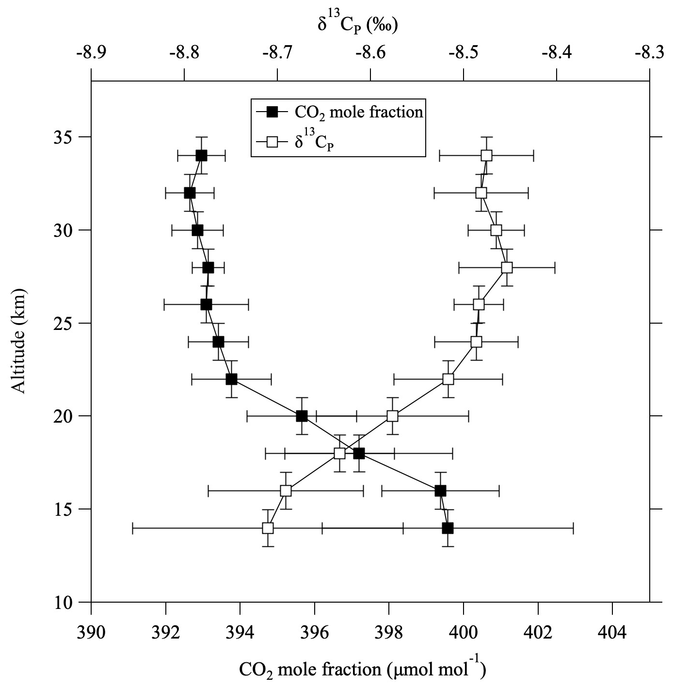
Figure 8 Vertical profiles of CO₂ mole fraction (closed squares) and stratospheric potential δ¹³C (δ¹³C_P, open squares) based on their averages in 11 vertical bins over the period 1985–2020. All values were detrended and normalized to values in August 2016.

If δ¹³C_P is truly a conserved quantity in the stratosphere, it should decrease over time with a time lag relative to the variation in the tropical upper troposphere. However, there are no long-term data records of δ¹³C values in CO₂ and CH₄ in the tropical upper troposphere. Therefore, we hypothetically synthesized a δ¹³C_P record in the tropical upper troposphere based on surface data observed at MLO and in the equatorial Pacific region by INSTAAR (Michel et al., 2025, 2023). In our previous study, we employed CO₂ mole fraction data obtained in the tropical upper troposphere using the Automatic Air Sampling Equipment in the Comprehensive Observation Network for TRace gases by AIrLiner (CONTRAIL) program (Machida et al., 2008; Sawa et al., 2008; Matsueda et al., 2015) to estimate the mean age of stratospheric air (Sugawara et al., 2018). A similar method was used in this study. We first estimated the average seasonal cycle of δ¹³CO₂ in the tropical upper troposphere from the observed seasonal cycle of the CO₂ mole fraction, assuming that the correlation between the seasonal cycles of the CO₂ mole fraction and δ¹³CO₂ in the upper troposphere was approximately −0.05 ‰ (µmol mol${}^{-\mathrm{1}}{)}^{-\mathrm{1}}$ (Nakazawa et al., 1993). The long-term δ¹³CO₂ trend was calculated from the observation data at MLO and then adjusted to match the observations in the equatorial Pacific region. The average seasonal cycles were then added to the long-term δ¹³CO₂ trend estimated in the equatorial Pacific region. The difference between δ¹³CO₂ values at the surface and those in the upper troposphere in the equatorial region is currently unknown. However, Sugawara et al. (2018) reported that the CO₂ and SF₆ ages in the TTL are 0.5–0.6 yr, consistent with the SF₆ age of 0–1.5 yr in the TTL based on Michelson Interferometer for Passive Atmospheric Sounding (Stiller et al., 2008). Taking this into account, we assumed the difference between surface and upper troposphere δ¹³CO₂ values in the equatorial region to be equivalent to 0.5 yr. Because systematic measurements of CH₄ mole fraction and δ¹³CH₄ in the upper troposphere were performed in the CONTRAIL program (Umezawa et al., 2012), the MLO data obtained by INSTAAR were adjusted to fit the CONTRAIL data in the equatorial upper troposphere to produce long-term records of CH₄ mole fraction and δ¹³CH₄ in the equatorial upper troposphere. Because the seasonal cycle of δ¹³CH₄ in the equatorial upper troposphere is not clear (Umezawa et al., 2012), the seasonal cycle was ignored in the calculation of the upper tropospheric δ¹³C_P. Since GS, i.e., 〈δ_G〉−〈δ_G〉₀, should be zero in the equatorial upper troposphere, tropospheric δ¹³C_P=δ¹³C_T.

As seen in Fig. 9, δ¹³CO₂ values did not differ significantly between the troposphere and the mid-stratosphere. However, the δ¹³C_P values calculated from observed values in the mid-stratosphere were, on average, about 0.14 ± 0.03 ‰ higher than those calculated for the tropical troposphere. This means that δ¹³C_P is conservative in the stratosphere and that the decreasing tropospheric δ¹³C_P trend through time propagates into the stratosphere with a time delay. Roughly calculated, this lag time is about 5 yr, consistent with the age of air estimated from CO₂ mole fractions (Appendix C) and the model calculation. If the mid-stratospheric δ¹³C_P values were shifted by −5 yr, they were in good agreement with the tropospheric δ¹³C_P trend (Fig. 9).

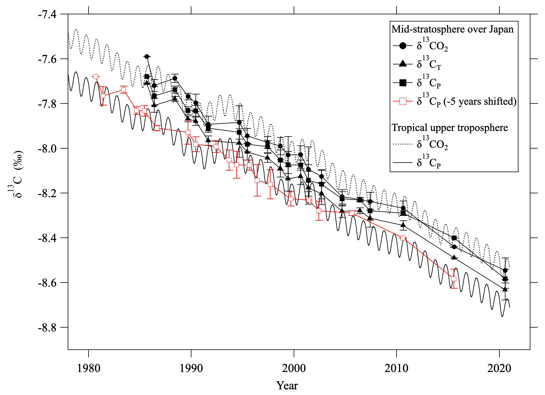
Figure 9 Average mid-stratospheric (>24 km altitude) values of δ¹³CO₂ (closed circles), δ¹³C_T (closed triangles), and δ¹³C_P (closed squares) over Japan. δ¹³CO₂ and δ¹³C_P in the tropical upper troposphere are shown by dashed and solid lines, respectively. Red squares show the mid-stratospheric δ¹³C_P shifted by −5.0 yr.

It is thus possible to estimate the mean age of air using δ¹³C_P, which can serve as an additional air age tracer. Therefore, we estimated the mean age of air not only from the CO₂ mole fraction but also from δ¹³C_P using a convolution method. Details of the age estimation method are described in Appendix C. The total uncertainty on individual δ¹³C_P ages was estimated to be ± 1.9 yr. This rather large uncertainty means that δ¹³C_P, with its smaller tropospheric secular change compared to other age tracers, was somewhat disadvantageous for age estimations. Because some of the δ¹³C_P values in the lower stratosphere showed high variability, with values lower than the tropospheric reference record, the convolution method could not provide reasonable age estimations for those data. We attributed these irregularities and low values to the large seasonal variations in the upper troposphere and the stratosphere–troposphere air exchange in the lower stratosphere. Therefore, only mid-stratospheric (>24 km altitude) data were taken into account for age estimations, and the average values of the mean age were calculated.

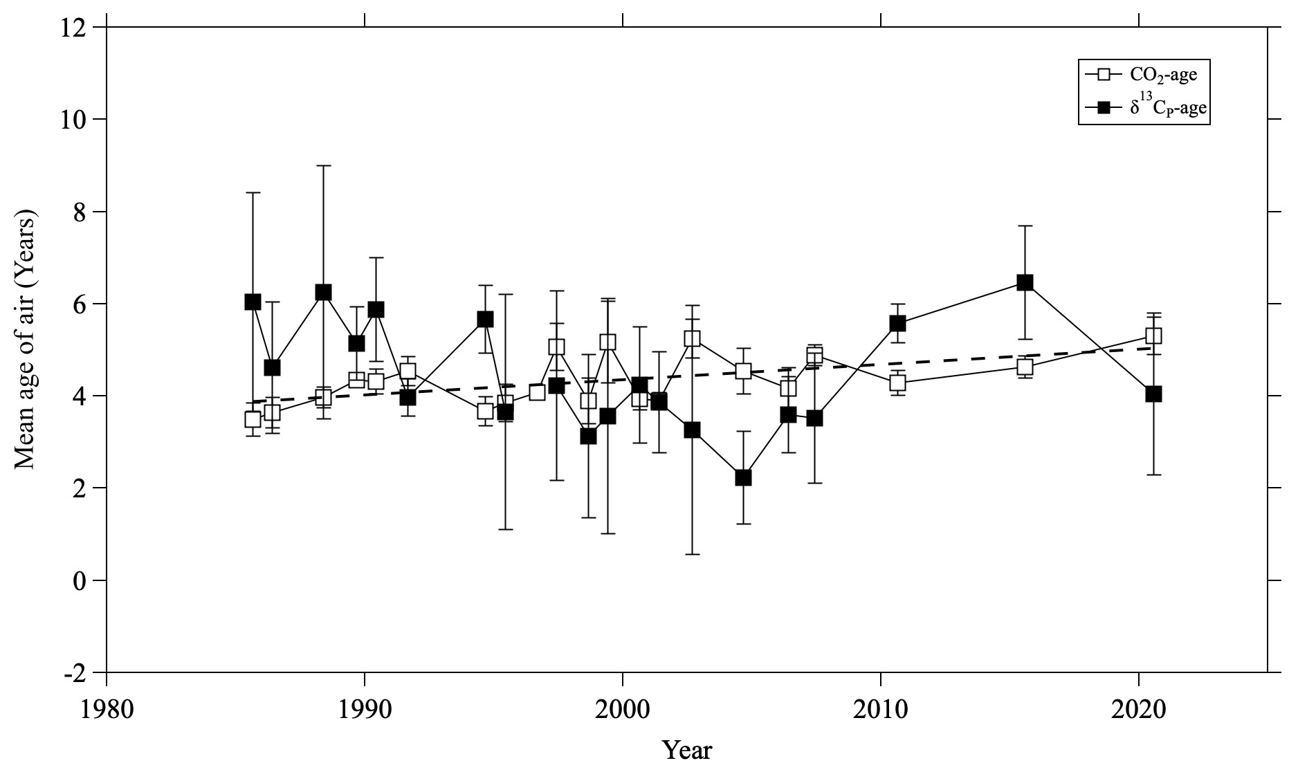
Figure 10 Temporal variations of averaged δ¹³C_P ages (closed squares) and CO₂ ages (open squares) in the mid-stratosphere (>24 km altitude) over Japan. The dashed line is a linear least-squares fit to the CO₂ ages. The linear fit to the δ¹³C_P age is not shown because the trend is not significant.

The results are shown in Fig. 10, along with the mean age calculated from the CO₂ mole fraction using the same method. The average δ¹³C_P and CO₂ ages were 5.5 ± 1.6 and 4.4 ± 0.6 yr, respectively. Because the uncertainty of the δ¹³C_P age was large, no significant difference was apparent between the two values. To examine the long-term trend of mean age, a linear function was fitted to both the CO₂ and δ¹³C_P age data using the least squares method. A slightly positive trend (0.04 ± 0.01 yr yr⁻¹) was observed for the CO₂ age, but no specific trend was observed for the δ¹³C_P age. It is important to note that our data were unevenly distributed over time, with sparse observations in recent years and more frequent observations before 2007. This made it difficult to clarify the exact 35 yr trend from our data alone. At present, the δ¹³C_P age has a relatively large uncertainty, making it unsuitable for use as an additional constraint for the age estimation. However, considering that the average δ¹³C_P age was estimated to be 5.5 ± 1.6 yr, the concept of stratospheric δ¹³C_P itself would be valid.

4 Conclusions

Previous studies on δ¹³CO₂ have mainly focused on observations in the troposphere and on elucidating the global CO₂ budget based on monitoring programs. However, little research has been performed on δ¹³CO₂ in the stratosphere, and the mechanisms of its distribution and variations are not fully understood. This study presented a comprehensive analysis of stratospheric δ¹³CO₂ obtained from balloon observations over Japan during the period 1985–2020. The following four factors were found to be important for understanding the variations of δ¹³CO₂ in the stratosphere. (1) Appropriate corrections for the MIE on ¹⁷O and ¹⁸O in isotopic analyses are essential. However, even after applying this correction, we found that the average values of δ¹³CO₂ in the northern mid-latitude mid-stratosphere and the tropical troposphere were almost identical, despite the secular decreasing δ¹³CO₂ trend and the expected time lag (age of air). We attributed this strange agreement to the other three factors: (2) airborne production of ¹³C-depleted CO₂ by the oxidation of CH₄ in the stratosphere, (3) GS of ¹²CO₂ and ¹³CO₂ in the stratosphere, and (4) propagation of the decreasing tropospheric δ¹³CO₂ trend into the stratosphere. Based on these considerations, we introduced “stratospheric potential δ¹³C” (δ¹³C_P) as a new concept and inspected δ¹³C_P in terms of the age of air. The average δ¹³C_P age was calculated to be 5.5 ± 1.6 yr for the period of 1985–2020. Because the δ¹³C_P age has larger uncertainties than the CO₂ age at present, it is difficult to refine the mean age estimation. However, δ¹³C_P in the mid-latitude mid-stratosphere decreased over time with a time delay and it was found to be quasi-conservative in the stratosphere.

The observation of numerous stratospheric air constituents, as in this study, requires the collection of a large amount of stratospheric air with a high-quality method and multi-component gas analyses of each air sample. GS of atmospheric constituents in the stratosphere was first revealed by our previous balloon observations, and this knowledge is indispensable for a better understanding of the variations of stratospheric δ¹³CO₂. The quality of the air samples is particularly important for observing GS in the mid-stratosphere, because even slight separations due to molecular diffusion during air sampling could prevent GS observations. At present, the only method capable of such sampling is our cryogenic air sampler.

The 2-D model reproduced the basic structure of stratospheric δ¹³CO₂ and elucidated the mechanisms governing δ¹³CO₂ behavior. However, our numerical model simulations remained insufficient because the mean age of stratospheric air could not be reproduced adequately without arbitrarily tuning the model. Accordingly, our model overestimated the effect of airborne CO₂ production via CH₄ oxidation because the reaction process was treated in a very coarse manner. To improve upon this model, it will be necessary to incorporate KIEs into all reactions related to stratospheric carbon. Although a two-dimensional model was used in this proof-of-concept study, a three-dimensional model is desirable for more realistic simulations in the future.

Appendix A: Gravitational separation of major atmospheric components

The gravitational separation (GS) of atmospheric components in the stratosphere was first reported from our balloon observations in Japan (Ishidoya et al., 2006, 2008a, 2013), in which the isotopic and elemental ratios of major atmospheric compositions, such as δ¹⁵N in N₂, δ¹⁸O in O₂, and δ(Ar $/$ N₂), were measured by mass spectrometry at the National Institute of Advanced Industrial Science and Technology (AIST; e.g., Ishidoya et al., 2006, 2008a; Sugawara et al., 2018). Technical aspects of our mass spectrometry analyses are described in detail in Ishidoya and Murayama (2014). In this study, we used δ¹⁵N, δ¹⁸O, and δ(Ar $/$ N₂) to evaluate GS, which are respectively defined as

$$\begin{array}{}\text{(A1a)}& {\mathit{\delta }}^{\mathrm{15}}\mathrm{N}={\displaystyle \frac{{\left[n\left({}^{\mathrm{15}}{\mathrm{N}}^{\mathrm{14}}\mathrm{N}\right)/n\left({}^{\mathrm{14}}{\mathrm{N}}^{\mathrm{14}}\mathrm{N}\right)\right]}_{\mathrm{sp}}}{{\left[n\left({}^{\mathrm{15}}{\mathrm{N}}^{\mathrm{14}}\mathrm{N}\right)/n\left({}^{\mathrm{14}}{\mathrm{N}}^{\mathrm{14}}\mathrm{N}\right)\right]}_{\mathrm{st}}}}-\mathrm{1},\end{array}$$

$$\begin{array}{}\text{(A1b)}& {\mathit{\delta }}^{\mathrm{18}}\mathrm{O}={\displaystyle \frac{{\left[n\left({}^{\mathrm{18}}{\mathrm{O}}^{\mathrm{16}}\mathrm{O}\right)/n\left({}^{\mathrm{16}}{\mathrm{O}}^{\mathrm{16}}\mathrm{O}\right)\right]}_{\mathrm{sp}}}{{\left[n\left({}^{\mathrm{18}}{\mathrm{O}}^{\mathrm{16}}\mathrm{O}\right)/n\left({}^{\mathrm{16}}{\mathrm{O}}^{\mathrm{16}}\mathrm{O}\right)\right]}_{\mathrm{st}}}}-\mathrm{1},\end{array}$$

and

$$\begin{array}{}\text{(A1c)}& \mathit{\delta }\left(\mathrm{Ar}/{\mathrm{N}}_{\mathrm{2}}\right)={\displaystyle \frac{{\left[n\left({}^{\mathrm{40}}\mathrm{Ar}\right)/n\left({}^{\mathrm{14}}{\mathrm{N}}^{\mathrm{14}}\mathrm{N}\right)\right]}_{\mathrm{sp}}}{{\left[n\left({}^{\mathrm{40}}\mathrm{Ar}\right)/n\left({}^{\mathrm{14}}{\mathrm{N}}^{\mathrm{14}}\mathrm{N}\right)\right]}_{\mathrm{st}}}}-\mathrm{1},\end{array}$$

where “sp” and “st” denote the sample and standard gases, respectively. The 1σ reproducibilities of our δ¹⁵N, δ¹⁸O, and δ(Ar $/$ N₂) measurements were ±2, ±5, and ±7 per meg, respectively, which was sufficient to detect GS in the stratosphere. Ishidoya et al. (2013) concluded that vertical variations of the isotopic ratios of major atmospheric components are dominated by differences in molecular mass, based on mass-dependent relationships among related molecules such as δ¹⁵N in N₂, δ¹⁸O in O₂, and the Ar $/$ N₂ ratio. Such GS in the stratosphere is known to be proportional to the mass difference, as would be expected for pure molecular diffusion, even though eddy diffusion obviously far exceeds molecular diffusion in the stratosphere. Therefore, GS can be expressed as

$$\begin{array}{}\text{(A2)}& \mathit{\delta }-{\mathit{\delta }}_{\mathrm{0}}=\mathrm{\Delta }m\times \left(\langle {\mathit{\delta }}_{\mathrm{G}}\rangle -\langle {\mathit{\delta }}_{\mathrm{G}}{\rangle }_{\mathrm{0}}\right),\end{array}$$

where Δm is the mass number difference, the suffix “0” refers to the value before GS occurs (i.e., corresponding to the relevant value in the upper troposphere), and 〈δ_G〉 is the average of δ values normalized to Δm=1 as reported by Ishidoya et al. (2013) and Sugawara et al. (2018). 〈δ_G〉 is defined by

$$\begin{array}{}\text{(A3)}& \langle {\mathit{\delta }}_{\mathrm{G}}\rangle ={\displaystyle \frac{\mathrm{1}}{\mathrm{3}}}\left[{\mathit{\delta }}^{\mathrm{15}}\mathrm{N}+{\mathit{\delta }}^{\mathrm{18}}\mathrm{O}/\mathrm{2}+\mathit{\delta }\left(\mathrm{Ar}/{\mathrm{N}}_{\mathrm{2}}\right)/\mathrm{12}\right].\end{array}$$

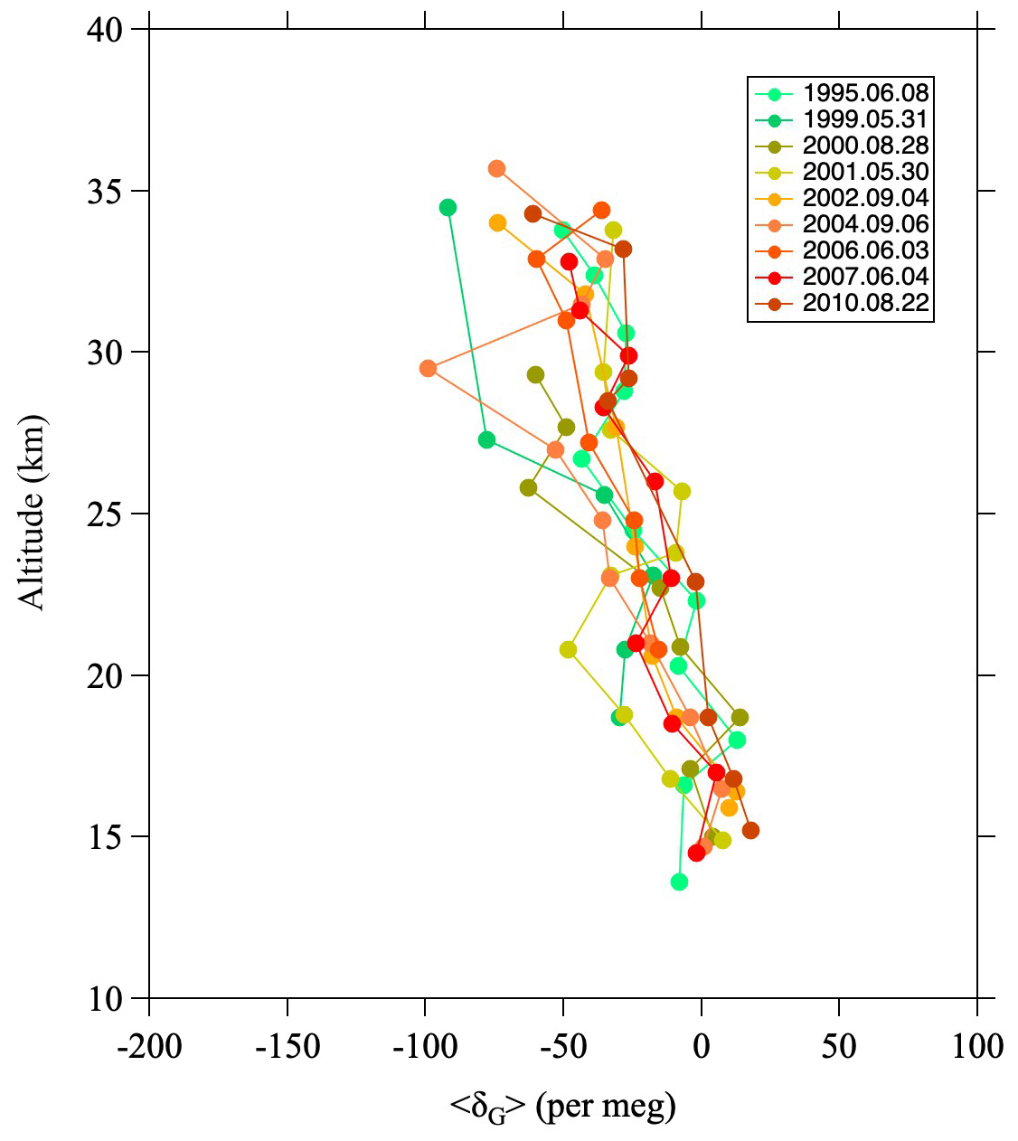
Figure A1 Vertical profiles of GS, 〈δ_G〉, observed over Japan (Ishidoya et al., 2013).

Figure A1 shows vertical profiles of 〈δ_G〉 obtained from balloon observations over Japan (Ishidoya et al., 2013). The value of 〈δ_G〉 decreases gradually with increasing altitude. By fitting a linear function to the vertical profiles, the average difference of 〈δ_G〉 between the lowermost and uppermost altitudes was found to be −66 ± 17 per meg. Here, it is important to mention the relationship between the GS of δ¹⁸O and photochemical processes. As mentioned in Sect. 2.2., in the stratosphere, O₃ and CO₂ are significantly enriched in ¹⁷O and ¹⁸O by MIEs associated with photochemical reaction processes. Because stratospheric O₂ molecules are the source of the ¹⁷O and ¹⁸O enrichment, δ¹⁷O and δ¹⁸O values of O₂ are thought to be lower in the stratosphere than in the troposphere due to photochemical processes. This assumption is crucial not only for the Dole–Morita effect, but also for the ¹⁷O budget of tropospheric O₂ (Bender et al., 1994; Luz et al., 1999; Luz and Barkan, 2011; Ishidoya et al., 2025). However, δ¹⁸O values of stratospheric O₂ measured in our balloon observations show a very large decrease, i.e., by approximately −130 per meg, at around 35 km that is almost entirely dominated by GS. This decrease is probably also due in part to photochemical effects, but their contribution should be negligible, amounting to only a few per meg (Ishidoya et al., 2025).

Appendix B: Two-dimensional model

We used a two-dimensional model of the middle atmosphere (SOCRATES) developed by the National Center for Atmospheric Research (NCAR; Huang et al., 1998; Park et al., 1999; Khosravi et al., 2002). The advantage of using this model is that we have already calculated ¹³C¹⁶O₂ and ¹²C¹⁶O₂ and examined stratospheric GS in our previous studies (Ishidoya et al., 2013; Sugawara et al., 2018). Therefore, we give only a brief description of the model calculation here. To reproduce GS, the molecular diffusion flux must be calculated. The vertical component of the molecular diffusion flux ($F_{m_i,z}$) is given by

$$\begin{array}{}\text{(B1)}& F_{m_i,z}=-D_{m_i}\left\{{\displaystyle \frac{\partial n_i}{\partial z}}+{\displaystyle \frac{m_i\mathrm{g}}{RT}}{n}_i+\left(\mathrm{1}+{\mathit{\alpha }}_{T_i}\right){\displaystyle \frac{\partial \left(\ln T\right)}{\partial z}}{n}_i\right\},\end{array}$$

where n_i, $D_{m_i}$, m_i, and ${\mathit{\alpha }}_{T_i}$ are the number density, molecular diffusion coefficient, molecular mass, and thermal diffusion factor of atmospheric constituent i, respectively, and g, R, and T are the gravitational acceleration, gas constant, and temperature, respectively (Banks and Kockarts, 1973). However, because the thermal diffusion flux is not important in this case, we ignored it in the model calculations. Because it is cumbersome to include all CO₂ isotopologues in the model calculations, only ¹²C¹⁶O₂ and ¹³C¹⁶O₂ were calculated independently in the model, and δ¹³CO₂ was approximated using the respective mole fractions of n(¹³C¹⁶O₂) and n(¹²C¹⁶O₂) as

$$\begin{array}{}\text{(B2)}& {\mathit{\delta }}^{\mathrm{13}}{\mathrm{CO}}_{\mathrm{2}}=\left({\displaystyle \frac{\mathrm{1}}{{}^{\mathrm{13}}{R}_{\mathrm{VPDB}}}}{\displaystyle \frac{n\left({}^{\mathrm{13}}{\mathrm{C}}^{\mathrm{16}}{\mathrm{O}}_{\mathrm{2}}\right)}{n\left({}^{\mathrm{12}}{\mathrm{C}}^{\mathrm{16}}{\mathrm{O}}_{\mathrm{2}}\right)}}-\mathrm{1}\right).\end{array}$$

Because δ¹³CO₂ has a large seasonal cycle in the troposphere, we used NOAA/GML and INSTAAR data to give latitude-dependent seasonal cycles as boundary conditions at the model surface. In addition, a secular decrease of δ¹³CO₂ in the troposphere was given by the MLO data (Michel et al., 2025). SOCRATES originally included a series of carbon reactions starting with CH₄ oxidation. Model calculations were repeated with and without GS, the secular trend and seasonal cycle of tropospheric δ¹³CO₂, and airborne CO₂ production, and comparisons were made between them (Fig. 2c). The chemical budget of CO₂ in SOCRATES is calculated as

$$\begin{array}{}\text{(B3)}& \begin{array}{rl}{\displaystyle \frac{d\left[{\mathrm{CO}}_{\mathrm{2}}\right]}{\mathrm{d}t}}& =k_{\mathrm{CO}+\mathrm{OH}}\left[\mathrm{CO}\right]\left[\mathrm{OH}\right]\\ & +k_{\mathrm{CO}+\mathrm{O}\left({}^{\mathrm{3}}\mathrm{P}\right)}\left[M\right]\left[\mathrm{CO}\right]\left[\mathrm{O}{(}^{\mathrm{3}}\mathrm{P}\right)]\\ & -J_{{\mathrm{CO}}_{\mathrm{2}}}\left[{\mathrm{CO}}_{\mathrm{2}}\right],\end{array}\end{array}$$

where k_CO+OH and $k_{\mathrm{CO}+\mathrm{O}\left({}^{\mathrm{3}}\mathrm{P}\right)}$ are the reaction rates of their respective chemical reactions, and M is the third body which carries off excess energy in a termolecular reaction. Because CO₂ photodissociation is important only above the mesosphere (e.g., Garcia et al., 2014), it was ignored in this study. KIEs in the CH₄–CO–CO₂ chain reaction were not included explicitly in these simulations but were rather treated in a coarse manner as follows. Simulations were performed with and without the chemical production of CO₂. Taking the CO₂ mole fractions simulated with (“wP”) and without chemical production (“nP”) to be n(CO₂)_wP and n(CO₂)_nP, respectively, the CO₂ mole fraction difference between the two simulations, n(CO₂)_wP−n(CO₂)_nP, was calculated as the apparent CO₂ production in the stratosphere. The apparent CO₂ production is distinct from the local production calculated in Eq. (B3) because it is an apparent value influenced by the accumulated chemical processes along the pathway of the air mass, including transport and mixing. A typical value of the apparent CO₂ production was simulated to be about 1.5 µmol mol⁻¹ at 35 km altitude in the mid-latitudes. Similarly, the δ¹³CO₂ value simulated excluding chemical CO₂ production was expressed by δ¹³CO_2,nP. After both these simulations, the δ¹³CO₂ value including airborne CO₂ sources from the CH₄ destruction, δ¹³CO_2,wP, was calculated as

$$\begin{array}{}\text{(B4)}& \begin{array}{rl}& {\mathit{\delta }}^{\mathrm{13}}{\mathrm{CO}}_{\mathrm{2},\mathrm{wP}}=\\ & {\displaystyle \frac{{\mathit{\delta }}^{\mathrm{13}}{\mathrm{CO}}_{\mathrm{2},\mathrm{nP}}\times n{\left({\mathrm{CO}}_{\mathrm{2}}\right)}_{\mathrm{nP}}+{\mathit{\delta }}^{\mathrm{13}}{\mathrm{CH}}_{\mathrm{4}\mathrm{\_}\mathrm{L}}\times \left[n{\left({\mathrm{CO}}_{\mathrm{2}}\right)}_{\mathrm{wP}}-n{\left({\mathrm{CO}}_{\mathrm{2}}\right)}_{\mathrm{nP}}\right]}{n{\left({\mathrm{CO}}_{\mathrm{2}}\right)}_{\mathrm{wP}}}}.\end{array}\end{array}$$

In this equation, δ¹³CH_{4_L} was calculated using Eq. (6) assuming apparent fractionation factors of 0.9889 and 0.9866 at lower (<24 km) and upper (>24 km) altitudes, respectively (see Sect. 3.2). Note that δ¹³CH_{4_L} values were estimated from the apparent fractionation factors by assuming Rayleigh distillation relationships between vertical profiles of CH₄ mole fraction and δ¹³CH₄. Therefore, these apparent fractionation factors differed from fractionation factors sensu stricto and were influenced by the accumulated KIEs along the pathway of the air mass, as with the apparent CO₂ production described above. Equation (B4) means that δ¹³CO₂ was simulated by combining the apparent fractionation factors estimated from observations with the apparent CO₂ production simulated by the model.

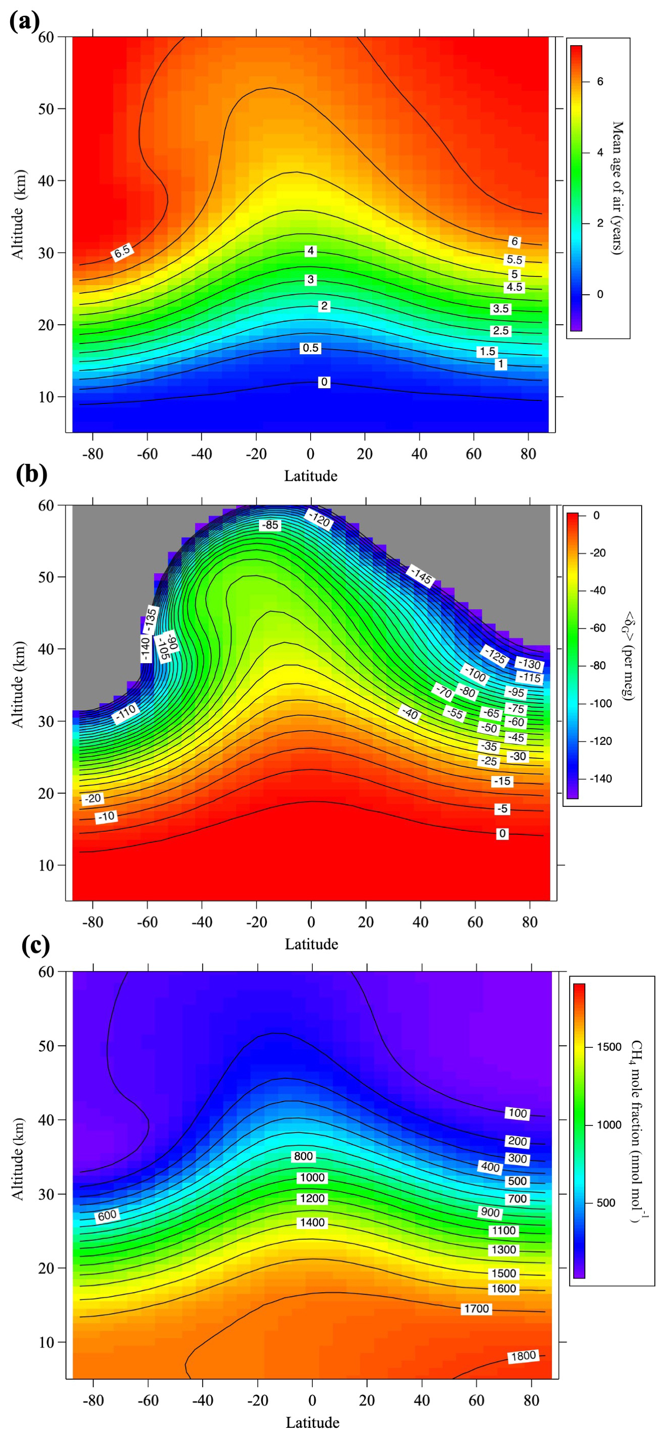
Figure B1 (a) Monthly average meridional distributions of the mean age of air for August 2016 calculated using the SOCRATES model. (b) As in (a), but for gravitational separation, 〈δ_G〉. Values lower than −150 per meg are shown in gray. (c) As in (a), but for the CH₄ mole fraction.

A virtual clock tracer was used to calculate the mean age of air. However, previous research has shown that the speed of the Brewer–Dobson circulation in SOCRATES is fast, leading to an underestimation of age of air. Therefore, similar to Sugawara et al. (2018), we reduced the mass stream function to approximate a realistic mean age, which also improved the reproduction of GS. The model results of GS reproduced well the almost linear decrease with increasing altitude above the tropopause in the observational results (Fig. A1). The model calculations were carried out over the 25 yr from 1995 to 2020. The monthly average meridional distribution of the mean air age, GS, and CH₄ mole fraction calculated by SOCRATES for August 2016 is shown in Fig. B1.

Appendix C: Age calculation

We estimated the mean age of air from δ¹³C_P using the same method that was previously applied to the CO₂ age estimation (Ray et al., 2017; Sugawara et al., 2018). The calculation of CO₂ age based on our balloon observations has been partly reported in previous studies (Engel et al., 2002; Ishidoya et al., 2013; Umezawa et al., 2025). The CO₂ ages estimated using air samples collected from 1995 to 2010 were published as supplementary data in Ishidoya et al. (2013). However, the method of age estimation was subsequently updated in Sugawara et al. (2018). In this study, we further improved the estimation method by correcting the δ¹³C_P and CO₂ mole fraction data for GS, creating a new 35 yr record. We estimated the mean age of air using the convolution method (Ray et al., 2017; Leedham Elvidge et al., 2018; Sugawara et al., 2018). This method has been described in detail by Sugawara et al. (2018), so only a brief explanation is given here. Hypothetical age spectra were used in the convolution method to estimate the mean age (Waugh and Hall, 2002). Expected temporal variations in the age tracer in the stratosphere, x(Γ,t), were calculated by convolution of the tropospheric reference curve, x₀(t), and the age spectrum, G(Γ,t):

$$\begin{array}{}\text{(C1)}& x\left(\mathrm{\Gamma },t\right)=\underset{t-T_{\mathrm{B}}}{\overset{t}{\int }}{x}_{\mathrm{0}}\left(t^{\prime }\right)G\left(\mathrm{\Gamma },t-t^{\prime }\right)\mathrm{d}{t}^{\prime },\end{array}$$

where T_B is the integration time interval. T_B should theoretically be ∞, but we truncated it to 20 yr for the calculations. Actual age spectra, G(Γ,t), are usually unknown. Therefore, we used the inverse Gaussian distribution (Waugh and Hall, 2002):

$$\begin{array}{}\text{(C2)}& G\left(\mathrm{\Gamma },t\right)={\left({\displaystyle \frac{{\mathrm{\Gamma }}^{\mathrm{3}}}{\mathrm{4}\mathit{\pi }{\mathrm{\Delta }}^{\mathrm{2}}{t}^{\mathrm{3}}}}\right)}^{\mathrm{1}/\mathrm{2}}\exp \left[{\displaystyle \frac{-\mathrm{\Gamma }{\left(t-\mathrm{\Gamma }\right)}^{\mathrm{2}}}{\mathrm{4}{\mathrm{\Delta }}^{\mathrm{2}}t}}\right].\end{array}$$

Here, Δ denotes the width of the age spectrum, and it was parameterized using the mean age (Γ), i.e., the ratio of moments, ${\mathrm{\Delta }}^{\mathrm{2}}/\mathrm{\Gamma }$. This value has usually been assumed to be 0.7 yr, as suggested by Hall and Plumb (1994) based on results from a general circulation model calculation, and it was used to estimate SF₆- and CO₂-derived mean ages in the northern mid- and high-latitude stratosphere (Engel et al., 2002). Recently, however, Fritsch et al. (2020) reported that a value of 1.25 yr is better for estimating ages from the SF₆ mole fraction. Therefore, we used 1.25 yr for the ratio of moments in this study. After calculating the convolutions, the mean age was determined by substituting the observed values, x_obs, into the inverse function, Γ (x, t). The convolutions are shown in Fig. C1 along with the calculated δ¹³C_P values.

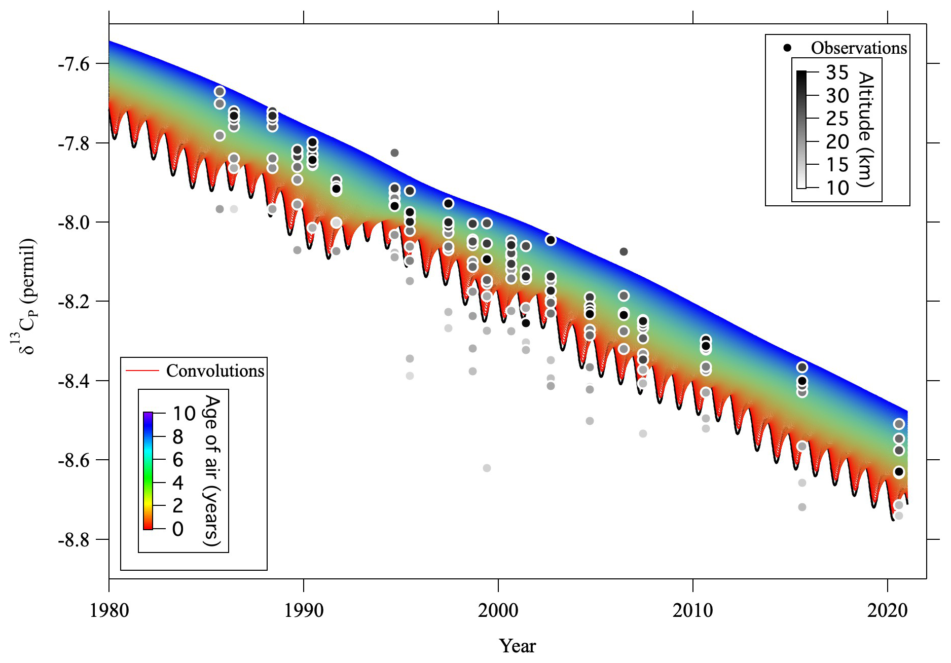
Figure C1 δ¹³C_P observed over Japan (circles) and convolutions of δ¹³C_P (colored lines) calculated from the tropospheric reference record and age spectrum. Observation altitudes of δ¹³C_P are indicated by the gray scale of the symbol colors.

It should be noted that uncertainties of individual mole fraction or isotopic ratio measurements, as well as of the tropospheric reference record, lead to uncertainties of individual age estimates (e.g., Leedham Elvidge et al., 2018). Umezawa et al. (2025) estimated a total uncertainty of 0.72 yr for our CO₂ ages. Similarly, we estimated the uncertainty for δ¹³C_P ages by adding normal pseudo-random numbers to all measured values and then calculating δ¹³C_P values using Eqs. (9) and (10). The uncertainty of the individual δ¹³C_P values was nearly identical to that of δ¹³C, ±0.02 ‰. On the other hand, the uncertainty of the tropospheric reference record for δ¹³C_P was calculated to be ±0.03 ‰. This value is in close agreement with the standard deviation obtained by applying curve fitting to the MLO δ¹³C data used as the tropospheric reference record. Taking into account all these uncertainties and the tropospheric trend of −0.026 ‰ yr⁻¹, the total uncertainty of the individual δ¹³C_P ages was estimated to be ±1.9 yr. The ratio of moments and its influence on age estimates have been examined in previous studies (e.g., Hauck et al., 2019; Nguyen et al., 2021). In this study, the mean age calculation was repeated as a sensitivity test for different ratios of moments ranging from 0.05 to 2.00 yr. As a result, the mean ages derived from δ¹³C_P were found to be within the observational uncertainties of the δ¹³C_P age. The δ¹³C_P age is larger than the CO₂ age (4.4 ± 0.6 yr) by about 1.1 yr on average. In this regard, δ¹³C_T was calculated from the observed CH₄ mole fraction and its δ¹³C, assuming a closed system (Eq. (9)). However, actual chemical processes do not occur in a closed system, and atmospheric mixing processes always result in apparent fractionation being smaller than true fractionation (Rahn et al., 1998; Kaiser et al., 2006; Toyoda et al., 2018). In this study, the isotopic effect of CH₄ oxidation was calculated based on the apparent fractionation factor. This would result in an underestimation of the CH₄ oxidation effect in Eq. (9) and an overestimation of the δ¹³C_P age. To solve this problem, it is necessary to explicitly incorporate the isotope effect of CH₄ into the model, which will be a future challenge.

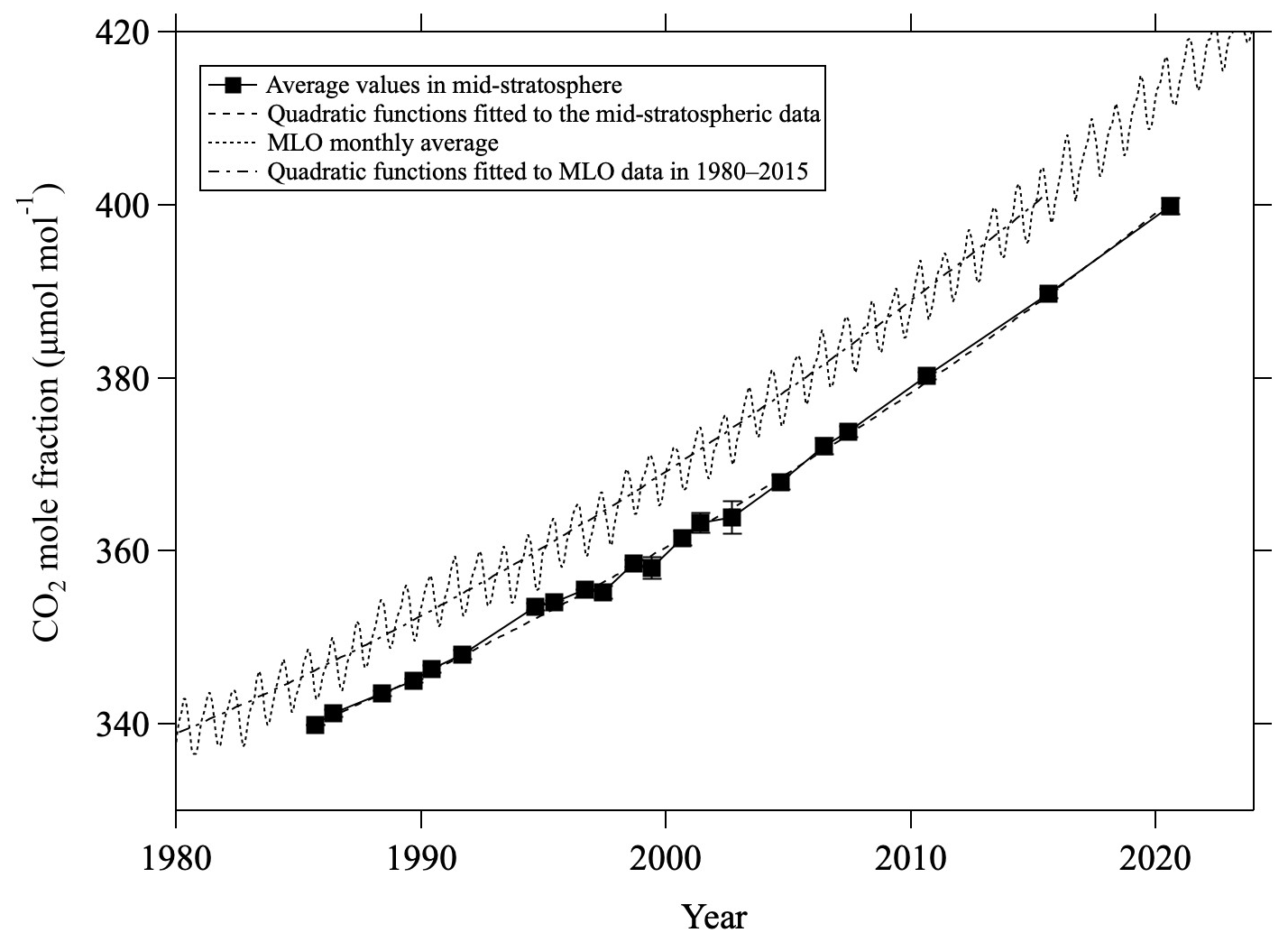
Figure C2 Average values of mid-stratospheric CO₂ mole fraction (>24 km altitude) over Japan (closed squares). Monthly average CO₂ mole fractions at Mauna Loa observed by NOAA/GML are shown by the dotted line. Quadratic functions fitted to the mid-stratospheric data (dashed line) and annual average MLO data from 1980 to 2015 (dashed-dotted line) are also shown.

Corresponding to the secular decrease of δ¹³CO₂, an increase in the CO₂ mole fraction was also clearly observed in the mid-stratosphere. To compare the temporal variations of the CO₂ mole fraction in the mid-stratosphere with those in the troposphere, the average values above 24 km altitude were calculated for each year, shown in Fig. C2 alongside the monthly average data obtained by NOAA/GML at MLO. The results of the sixth WMO/IAEA Round Robin Comparison Experiment showed that our CO₂ mole fraction values were approximately 0.2 µmol mol⁻¹ higher than the NOAA/GML values on the WMO-CO2-X2007 scale; accordingly, our CO₂ mole fraction values are plotted in Fig. C2 only after subtracting 0.2 µmol mol⁻¹. The CO₂ mole fraction in the mid-stratosphere over Japan increased monotonically and reached about 400 µmol mol⁻¹ in 2020, lagging behind that at MLO by about 5 yr. The average rate of change of the CO₂ mole fraction in the mid-stratosphere was calculated to be 1.68 ± 0.04 µmol mol⁻¹ yr⁻¹ by applying the least-squares method to the observed values. However, this increasing trend was not linear, gradually steepening over the last 40 yr. Therefore, a quadratic function of the form n(CO${}_{\mathrm{2}})=K_{\mathrm{0}}+(K_{\mathrm{1}}\times t)+(K_{\mathrm{2}}\times t^{\mathrm{2}}$) would better represent the observed variations. Here, t (years) is the elapsed time since 1980. The coefficients of the CO₂ mole fraction in the mid-stratosphere, K₀, K₁, and K₂, were calculated to be 333.7, 1.0448, and 0.0147 55, respectively. The standard deviation of residuals was 0.8 µmol mol⁻¹. The same procedure was applied to the annual mean CO₂ mole fractions at MLO for the period 1980–2015, considering a time lag of 5 yr between the mid-stratosphere and the troposphere. The coefficients K₀, K₁, and K₂ for the MLO data were calculated to be 338.85, 1.2307, and 0.0145 77, respectively. As shown in Fig. C2, the two quadratic functions thus obtained agreed well to within ±0.7 µmol mol⁻¹. This result suggests that even temporal changes in the rate of increase in the troposphere propagate to the mid-stratosphere with a certain time delay.

As described in the main text, the influences on CO₂ production of CH₄ oxidation and GS should be considered to precisely estimate the CO₂ age. Therefore, the CO₂ mole fraction was corrected as follows. At first, the tropical upper tropospheric CH₄ data, $x_{{\mathrm{CH}}_{\mathrm{4}}\mathrm{\_}\mathrm{tp}}\left(t\right)$, were created by adjusting the annual mean data at MLO to fit the CONTRAIL data in the tropical upper troposphere (Umezawa et al., 2012). Then, we corrected x_obs as

$$\begin{array}{}\text{(C3)}& \begin{array}{rl}{x}_{\mathrm{cor}}\left(t\right)& =x_{\mathrm{obs}}\left(t\right)-\left[x_{{\mathrm{CH}}_{\mathrm{4}}\mathrm{\_}\mathrm{tp}}\left(t-\mathrm{\Gamma }\right)-x_{{\mathrm{CH}}_{\mathrm{4}}\mathrm{\_}\mathrm{obs}}\left(t\right)\right]\\ & -{\mathrm{\Delta }}_{\mathrm{G}}\left(x_{\mathrm{obs}}\left(t\right)\right),\end{array}\end{array}$$

where x_cor and $x_{{\mathrm{CH}}_{\mathrm{4}}\mathrm{\_}\mathrm{obs}}$ denote the corrected CO₂ mole fraction and observed CH₄ mole fraction, respectively. Δ_G is the correction for GS (see Sect. 3.3.). The CO₂ mole fractions corrected for CH₄ oxidation and GS are shown with the convolutions in Fig. C3. Finally, the CO₂ age was determined as ${\mathrm{\Gamma }}_{{\mathrm{CO}}_{\mathrm{2}}}=\mathrm{\Gamma }\left(x_{\mathrm{cor}},t\right)$. We note that Eq. (C3) contains the mean age of air, Γ, because the CH₄ mole fraction in the troposphere has increased with time and CH₄ is destroyed over the air transport pathway from the tropical upper troposphere to the observation altitude in the stratosphere. Therefore, ${\mathrm{\Gamma }}_{{\mathrm{CO}}_{\mathrm{2}}}$ was solved iteratively by starting from ${\mathrm{\Gamma }}_{{\mathrm{CO}}_{\mathrm{2}}}=\mathrm{0}$. This iteration converged sufficiently after the second time of ${\mathrm{\Gamma }}_{{\mathrm{CO}}_{\mathrm{2}}}$ calculation. The vertical profiles of ${\mathrm{\Gamma }}_{{\mathrm{CO}}_{\mathrm{2}}}$, corresponding to CO₂ age, are shown in Fig. C4.

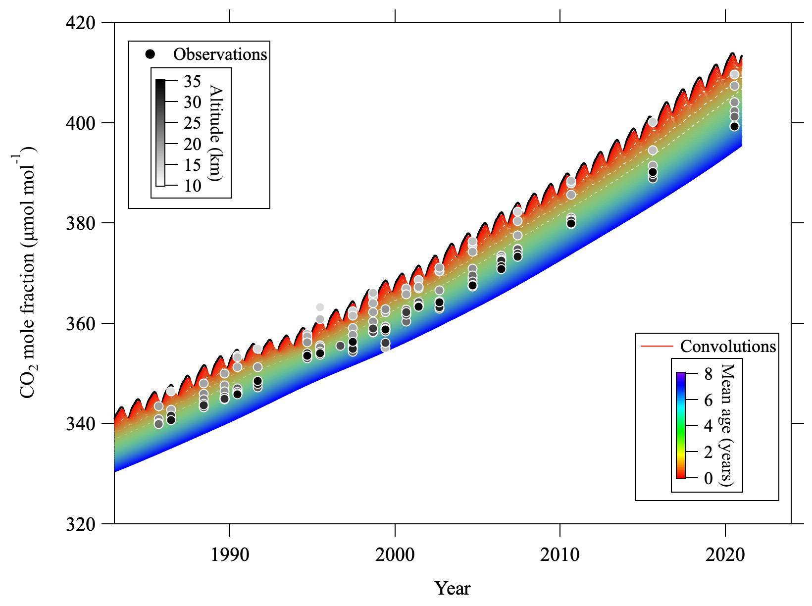
Figure C3 CO₂ mole fractions observed over Japan (circles) and convolutions (colored lines) calculated from the tropospheric reference record and age spectrum. Observation altitudes of the CO₂ mole fraction are indicated by the gray scale of the symbol colors. Note that the CO₂ mole fractions plotted have been corrected for CH₄ oxidation and GS.

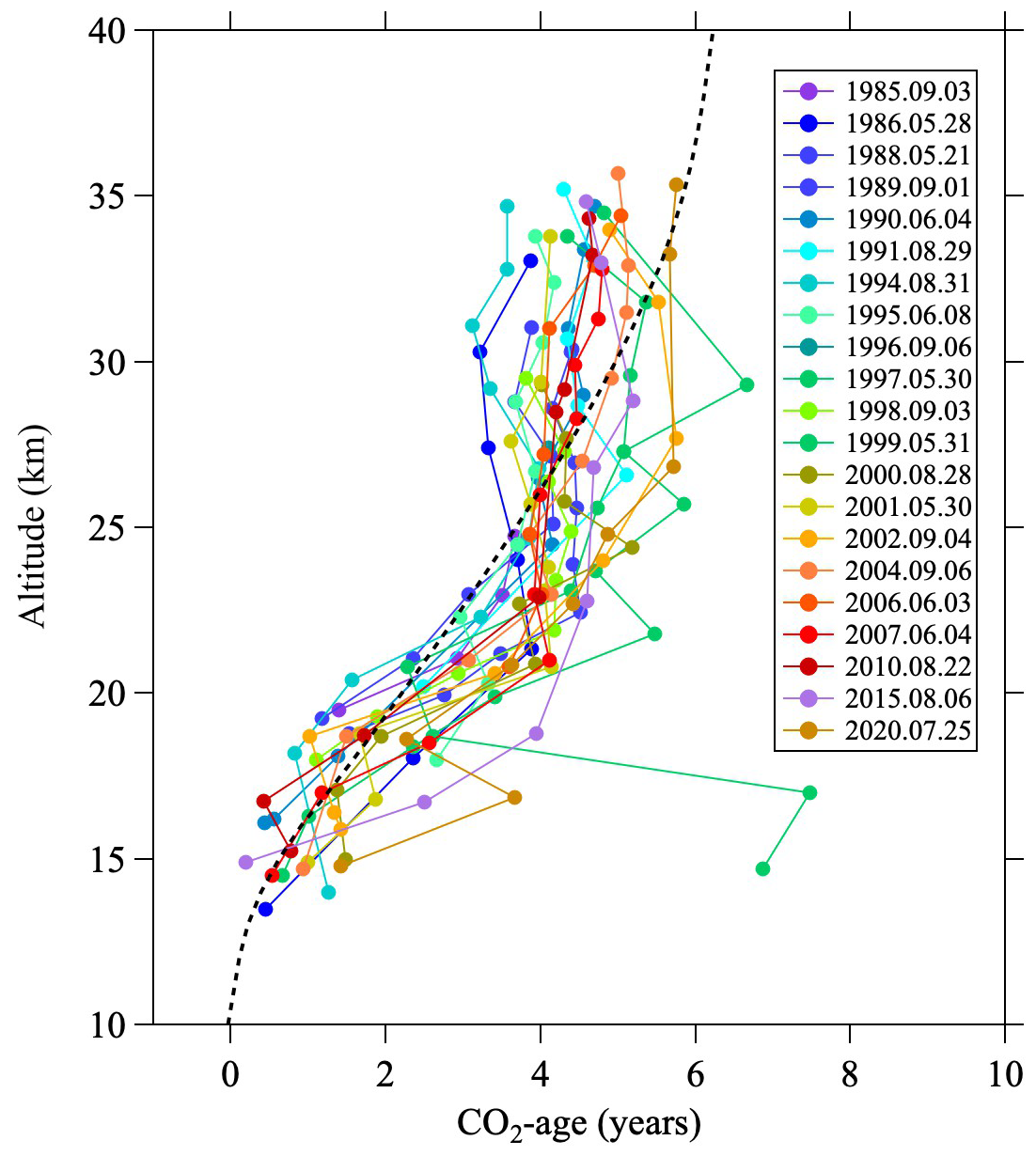
Figure C4 Vertical profiles of the CO₂ age calculated from CO₂ mole fractions from 1985 to 2020. The monthly average vertical profile of the mean age of air for August 2016 calculated using the SOCRATES model is shown by the dashed line.