Investigating the ability of satellite occultation instruments to monitor possible geoengineering experiments

Solar radiation management is a method in the field of geoengineering that aims to modify the Earth's shortwave radiation budget. One idea is to inject sulfur dioxide or sulfuric acid into the stratosphere, where sulfate aerosols are then formed. Such experiments can probably be observed, for example, with satellite occultation instruments like SAGE III/ISS. The aim of the current study is to analyse, using MAECHAM-HAM simulations and retrievals with the radiative transfer program SCIATRAN, whether it is possible to detect the formed stratospheric aerosols from emissions of 1 and 2 Tg S yr⁻¹ (sulfur per year) with the currently active satellite occultation instruments, taking into account an error estimate that is as realistic as possible. If these smaller amounts of sulfur are detectable, larger amounts will also be detectable. The calculations show that, considering the natural variability and the assumptions made here, the stratospheric aerosols formed from emissions of 1 and 2 Tg S yr⁻¹ in the quasi-steady-state phase can be detected, which is not the case in the first month of the 2-year initial phase.

1 Introduction

Geoengineering, also known as climate engineering, comprises methods and technologies that aim to deliberately change the climate system in order to mitigate the consequences of climate change (IPCC, 2013). One method is solar radiation management (SRM), which aims at modifying the shortwave radiation budget in the climate system by increasing the planetary albedo (IPCC, 2013). The injection of sulfur dioxide into the stratosphere (stratospheric aerosol injection, SAI) is one idea of SRM (e.g. Budyko, 1977; Crutzen, 2006), mimicking the effects of large volcanic eruptions where extensive amounts of sulfur dioxide reach the stratosphere. The corresponding radiative forcing of the formed sulfate aerosols depends on the injected amount of sulfur dioxide. Another idea is the injection of sulfuric acid (H₂SO₄) into the stratosphere (e.g. Vattioni et al., 2019; Janssens et al., 2020; Weisenstein et al., 2022) or carbonyl sulfide (COS) (e.g. Quaglia et al., 2022).

Note that the exact values of the resulting radiative forcing for the same injection rate may vary depending on the model and set up used (e.g. Niemeier and Tilmes, 2017; Laakso et al., 2022). Simulations with MAECHAM-HAM show that a continuous injection of 10 Tg S yr⁻¹ at an altitude of 60 hPa leads to a top of the atmosphere radiative forcing of −(1.79–2.06) W m⁻² (Niemeier and Timmreck, 2015). However, it was shown that the forcing efficiency (ratio of sulfate aerosol forcing to injection rate) decreases with increasing injection rate (e.g. Heckendorn et al., 2009; Niemeier and Timmreck, 2015).

SAI is strongly debated, especially the research gaps (e.g. Haywood et al., 2025). However, with progressing climate change and increasing costs and damage, a deployment may become more and more likely. SAI is supposed to be relatively cheap (e.g. Moriyama et al., 2017), and companies or startups may see an option to earn money with SAI (e.g, “Make sunsets” company (Make sunsets, 2024)). Therefore, it is very important to be able to observe relatively small amounts of sulfur aerosols in the atmosphere.

One potential way to monitor possible future deployment of SAI is the use of satellite instruments. The SAGE III/ISS (Stratospheric Aerosol and Gas Experiment III) instrument, mounted on the International Space Station (ISS), is a currently operating satellite solar occultation instrument. It measures the attenuation of solar radiation due to scattering and absorption of atmospheric components such as ozone, nitrogen dioxide, water vapour, and aerosols. A description of the solar occultation measurement technique can be found in, for example, McCormick et al. (1979). The instrument observes around 15 sunrises and 15 sunsets in 24 h and covers a possible latitude range between 70° S and 70° N (NASA, 2022). SAGE III/ISS has 12 spectral channels, of which 9 cover aerosols as target species. The nine specific wavelengths are 384, 448, 520, 601, 676, 755, 869, 1021, and 1543 nm (NASA, 2022).

The aim of the current study is to investigate whether it is possible to detect stratospheric aerosols formed from small amounts (in the context of possible geoengineering experiments) of sulfur artificially and continuously injected into the stratosphere. Here 1 and 2 Tg S yr⁻¹ are considered, which results in a much lower sulfate injection per time compared to a volcanic eruption with the same injected amount, using a satellite solar occultation instrument, like SAGE III/ISS. It is assumed that if these smaller amounts of sulfur (in the context of possible geoengineering experiments) are detectable, larger amounts will also be detectable. Although 1 and 2 Tg S yr⁻¹ do not have a significant climatic effect, about −0.3 and −0.6 W m⁻² (Niemeier and Timmreck, 2015), these emission rates were chosen to see whether it is possible to detect even these small amounts, taking into account an aerosol extinction retrieval error estimate that is as realistic as possible. This is especially the case in view of the fact that the continuously injected sulfur amounts of 1 and 2 Tg S yr⁻¹ lead to much lower injection amounts per time compared to a volcanic eruption with the same amount injected. For this purpose, MAECHAM-HAM simulation results for different SRM scenarios were used. These simulation results provided aerosol extinction coefficients at 500 and 550 nm for an altitude range of 10–27 km. The aerosol extinction coefficients were used to perform transmission calculations with SCIATRAN from the perspective of a typical solar occultation instrument, which were then used for the subsequent retrieval of the stratospheric aerosol extinction profiles using SCIATRAN. A sensitivity study, an error analysis, and the analysis of natural variability are then carried out to answer the question about the detectability of the geoengineering experiment. Note that although the following analyses examine the detectability for a typical satellite occultation instrument such as SAGE III/ISS, the SAGE retrieval algorithm was not used.

The paper is structured as follows. Section 2 describes the procedure regarding the MAECHAM-HAM simulations, as well as the transmission calculations and the retrievals using SCIATRAN. Section 3 provides an overview of the results, followed by the discussion and conclusions.

2 Methodology

2.1 MAECHAM-HAM model simulations

The evolution and distribution of sulfate aerosols were simulated with the middle atmosphere (MA) version of the ECHAM general circulation model (GCM) (MAECHAM; Giorgetta et al., 2006). MAECHAM was applied with a grid size of about 1.8°×1.8°, specifically the spectral truncation at wavenumber 63 (T63), and 95 vertical layers up to 0.01 hPa (about 80 km). The model solves prognostic equations for temperature, surface pressure, vorticity, divergence, and phases of water. MAECHAM (hereafter ECHAM) was interactively coupled to the prognostic modal aerosol microphysical Hamburg Aerosol Model (HAM) (Stier et al., 2005), which calculates the formation of sulfate aerosols including nucleation, accumulation, condensation and coagulation, and their removal processes by sedimentation and deposition. HAM has been adapted to stratospheric conditions, considering, for example, that the temperature range for the nucleation processes is valid for low stratospheric temperature and that the width of the mode bins (sigma) differs from the sigma in the troposphere (Kokkola et al., 2009; Niemeier et al., 2009; Niemeier and Timmreck, 2015). We prescribe reactive gases (e.g. ozone, nitrogen oxides, hydroxyl radical – OH) and photolysis rates of carbonyl sulfide (OCS), H₂SO₄, SO₂, SO₃, and O₃ on a monthly average basis. The initial conversion of SO₂ to H₂SO₄ is simulated with a simple stratospheric sulfur chemistry scheme, which is applied above the tropopause (Timmreck, 2001; Hommel et al., 2011).

The model simulates the related dynamical processes and generates the quasi-biennial oscillation in the stratosphere. The model is not coupled to an ocean model. We run the model with prescribed sea surface temperatures (SSTs) and sea ice, set to climatological values (Hurrell et al., 2008), averaged over the AMIP (Atmospheric Model Intercomparison Project) period 1950 to 2000 that does not change due to SAI. Besides the prescribed SSTs, the model is running freely. It calculates the dynamical processes following the equations in the GCM. No nudging, i.e. relaxing the prognostic variables toward an atmospheric reference state (e.g. ERA5 data), is applied.

The solar radiation scheme in ECHAM has 4 spectral bands: 1 for the visible and ultraviolet and 3 for the near-infrared. The longwave radiation scheme has 16 spectral bands (see Stier et al., 2005). Values for single-scattering albedo and asymmetry factor are taken from a look-up table, precalculated with Mie calculations, to save computation time.

The direct radiative effect of sulfate aerosol is included for both solar (shortwave, SW) and terrestrial (longwave, LW) radiation and coupled to the ECHAM radiation scheme. The model diagnoses the instantaneous aerosol radiative forcing via a double radiation call, once with aerosols and once without aerosols. The aerosols absorb near-infrared and LW radiation, which heats the stratosphere and dynamically influences the resulting processes. This model has already been successfully applied in previous climate engineering studies (Niemeier and Schmidt, 2017; Niemeier et al., 2020). The cooling of the troposphere is included as well. As we use climatological SSTs, the surface cooling of the sulfate aerosols is seen in the model over land only, not over the oceans. The latter would require a coupled ocean model.

Simulations were performed with 1 and 2 Tg S yr⁻¹. SO₂ was injected continuously at an altitude of 60 hPa (≈19 km) into one grid box of 2.8°×2.8° centred on the Equator at 121° E. This study uses data of the initial phase, i.e. the first 2 years, and of the quasi-steady-state phase, an average over 3 years (years 12 to 15). We performed a single simulation over several years. The injections for SAI ran for 15 years. For our study, we took 3 years at the end of these simulations and averaged them over time. This is similar to previous simulations and publications, e.g. Niemeier et al. (2020) and Weisenstein et al. (2022), where 3-year averages were also used. Figure A1 illustrates the time series of the global sulfate burden, showing that the steady-state phase is reached after 2 years. We used the early phase to include sulfate levels below the steady-state level to see if we could detect sulfate even earlier. At this point, the goal was not to use a stabilized result. The aim was to find a lower threshold at which detection would be possible.

The model output of the 95 levels was interpolated to provide aerosol extinction coefficients at 500 and 550 nm between 10–27 km, in 1 km steps. The provided aerosol extinction coefficient profiles are monthly averages.

In the following, the months of January and July are analysed for the latitude range of 85° S to 85° N, in 10° steps.

2.2 Simulations and retrievals with SCIATRAN

The SCIATRAN radiative transfer model was developed by the Institute of Environmental Physics at the University of Bremen, Germany (Rozanov et al., 2014). SCIATRAN was originally designed for satellite-based data retrieval. More information can be found at https://www.iup.uni-bremen.de/sciatran/ (last access: 30 April 2025).

Based on the ECHAM simulation results, in this case aerosol extinction coefficients for an altitude range of 10 to 27 km for 500 and 550 nm, the aerosol extinction coefficients at 520 nm were first calculated using the Ångström parameterization. Using the aerosol extinction coefficients at 520 nm, the corresponding transmission values for a solar occultation observation geometry were simulated with the SCIATRAN radiative transfer model, which were then used for the retrieval with SCIATRAN to retrieve the corresponding aerosol extinction profiles. More details are provided below.

2.2.1 Transmission calculations

Using the aerosol extinction coefficients at 500 and 550 nm from the ECHAM model simulations, the aerosol extinction coefficients at 520 nm were first calculated using the Ångström parameterization, since this is one of the spectral channels of SAGE III/ISS for aerosols as target species (NASA, 2022). For this purpose, the Ångström exponents, α, were calculated from the given aerosol extinction coefficients k₅₀₀ and k₅₅₀, and the aerosol extinction coefficients at 520 nm (k₅₂₀) were then determined as follows (Ångström, 1929):

$$\begin{array}{}\text{(1)}& k_{\mathrm{520}}=k_{\mathrm{500}}{\left({\displaystyle \frac{\mathrm{520}}{\mathrm{500}}}\right)}^{-\mathit{\alpha }},\end{array}$$

with

$$\begin{array}{}\text{(2)}& \mathit{\alpha }=-{\displaystyle \frac{\ln \left(\frac{k_{\mathrm{550}}}{k_{\mathrm{500}}}\right)}{\ln \left(\frac{\mathrm{550}}{\mathrm{500}}\right)}}.\end{array}$$

The exact values of α depend on the considered month, latitude, and injection scenario. For example, for January, 45° N, and background (0 Tg S yr⁻¹), the values are between ≈1.0 and 2.2, depending on the altitude. To calculate the corresponding transmission values through the Earth's atmosphere at 520 nm, the SCIATRAN radiative transfer model (version 4.7) was used (Rozanov et al., 2014). In the transmission modelling mode (solar/lunar occultation mode), the direct solar radiation transmitted through the spherical Earth's atmosphere is simulated. Atmospheric refraction was also considered in the simulations. The vertical profiles of pressure, temperature, and trace gases required for the simulations were taken from the implemented climatological database, which is based on a 3-D chemical transport model (Sinnhuber et al., 2003). Further input parameters for the transmission calculations with SCIATRAN are listed in Table 1.

Table 1 Input parameters for the transmission calculations with SCIATRAN.

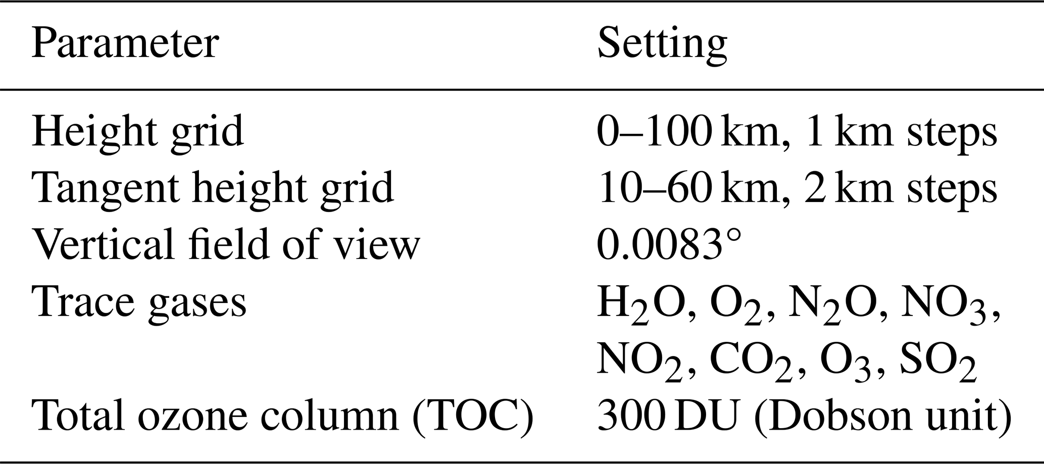
The input parameters, such as those relating to the viewing geometry, are selected so that they correspond to an imaginary satellite occultation instrument, like SAGE III/ISS, with a satellite altitude of 400 km. Output of the simulations with SCIATRAN are transmission values at 520 nm for the tangent heights of 10–60 km, in 2 km steps (compare Table 1).

2.2.2 Retrieval

For the retrieval of the extinction profiles at 520 nm, the retrieval algorithm in SCIATRAN 4.7 was used, which is not publicly available. A description of the retrieval algorithm can be found in Rozanov et al. (2011). The retrieval approach is the regularized inversion with the optimal estimation method.

The linearized inverse problem is formulated as follows:

$$\begin{array}{}\text{(3)}& \mathit{y}=F\left({\mathit{x}}_{\mathrm{a}}\right)+\mathbf{K}(\mathit{x}-{\mathit{x}}_{\mathrm{a}}),\end{array}$$

with y as the data vector (or measurement vector), containing the logarithms of the transmission values at 520 nm. F is the radiative transfer operator, x_a the a priori state vector, K the weighting function matrix, and x the state vector (to be retrieved). The a priori state vector x_a is kept constant over the iteration steps. The (approximate) solution of the inverse problem (Eq. 3) is obtained by minimizing the following equation:

$$\begin{array}{}\text{(4)}& {∥F\left({\mathit{x}}_{\mathrm{a}}\right)+K(\mathit{x}-{\mathit{x}}_{\mathrm{a}})-y∥}_{{\mathbf{S}}_{\mathit{ϵ}}^{-\mathrm{1}}}^{\mathrm{2}}+{∥(\mathit{x}-{\mathit{x}}_{\mathrm{a}})∥}_{{\mathbf{S}}_{\mathrm{a}}^{-\mathrm{1}}}^{\mathrm{2}}.\end{array}$$

Here S_ϵ is the noise covariance matrix and S_a the a priori covariance matrix. Since the inverse problem is not linear, the Gauss–Newton iterative approach is used to formulate the solution for each iteration step x_i+1 as follows:

$$\begin{array}{}\text{(5)}& \begin{array}{rl}{x}_{\mathrm{i}+\mathrm{1}}& ={\mathit{x}}_{\mathrm{a}}+{\left({\mathbf{K}}_i^T{\mathbf{S}}_{\mathit{ϵ}}^{-\mathrm{1}}{\mathbf{K}}_i+{\mathbf{S}}_{\mathrm{a}}^{-\mathrm{1}}\right)}^{-\mathrm{1}}{\mathbf{K}}_i^T{\mathbf{S}}_{\mathit{ϵ}}^{-\mathrm{1}}\left(y-F\left(x_i\right)\right.\\ & \left.+{\mathbf{K}}_i(x_i-{\mathit{x}}_{\mathrm{a}})\right).\end{array}\end{array}$$

More detailed information on the retrieval algorithm can be found in Rozanov et al. (2011, Sect. 3.4.2).

Table 2 shows the relevant input parameters for the retrieval. Note that for the purpose of clarity some of the input parameters that are already listed in Table 1 have also been added here. In addition, the calculated transmission values at 520 nm (Sect. 2.2) for the corresponding latitudes and months were used as data input. The retrieval was restricted to the altitude range of the aerosol extinction coefficients provided (see Sect. 2.1), i.e. from 10 to 27 km. Background aerosol extinction coefficient profiles at 520 nm corresponding to the latitude and month were used as a priori information. These profiles originate from the ECHAM model simulations for 0 Tg S yr⁻¹ (compare Sect. 2.1).

Table 2 Relevant input parameters for the retrievals with SCIATRAN.

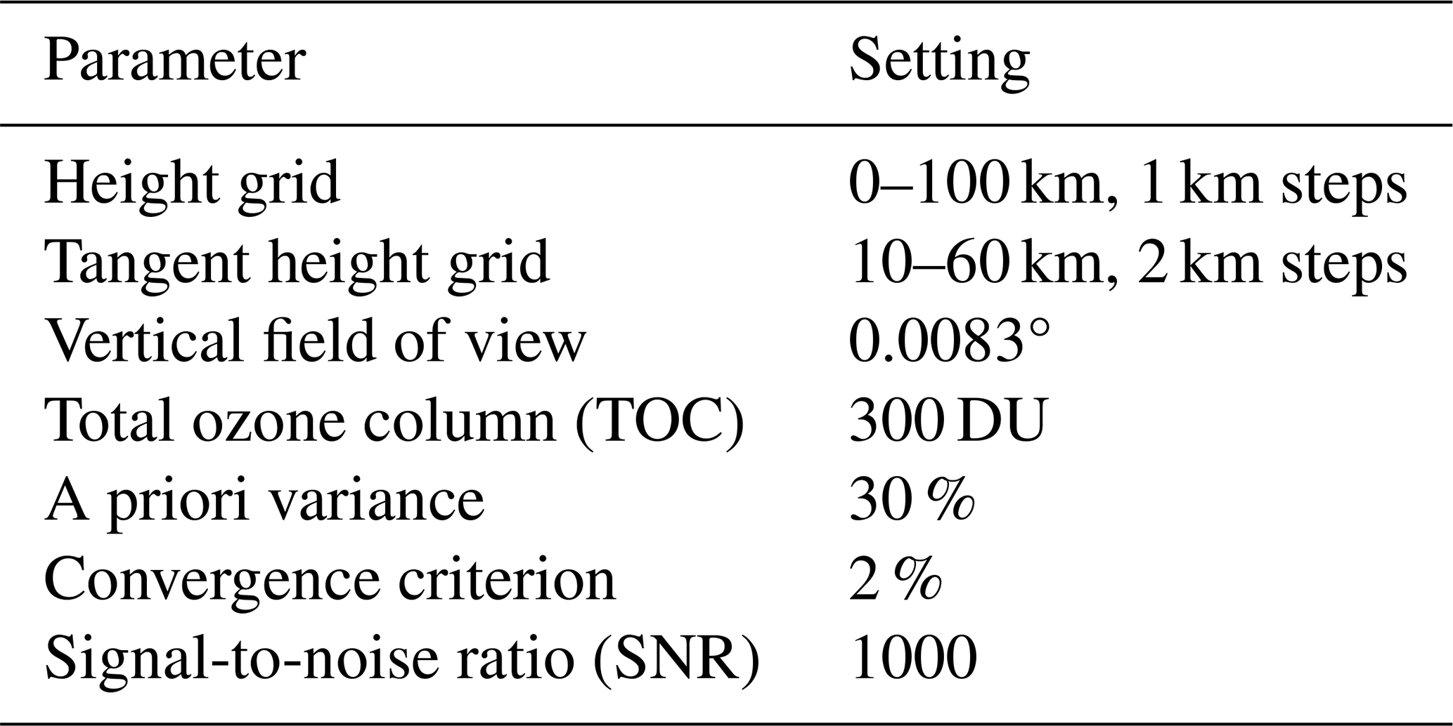
As already mentioned in Sect. 2.1, the retrievals were carried out for the latitudes 85° S to 85° N, in 10° steps for January and July (for the quasi-steady-state phase data) and January (for the initial-phase data). Output of the retrieval with SCIATRAN here is, among other data output files, the retrieved aerosol extinction profile at 520 nm.

3 Results and discussion

Figure 1 shows the extinction coefficients at 550 nm for January (Jan) to December (Dec) based on the ECHAM model simulations for the injection of 1 Tg S yr⁻¹ for the quasi-steady-state phase and the initial phase, demonstrating the differences between these two phases. The upper panel (a) of Fig. 1 displays ECHAM simulation results of the first year of the initial phase, and the lower panel (b) displays results of the quasi-steady-state phase. As previously described, the initial phase data include the first 2 years, and the quasi-steady-state phase data include an average over 3 years (years 12 to 15).

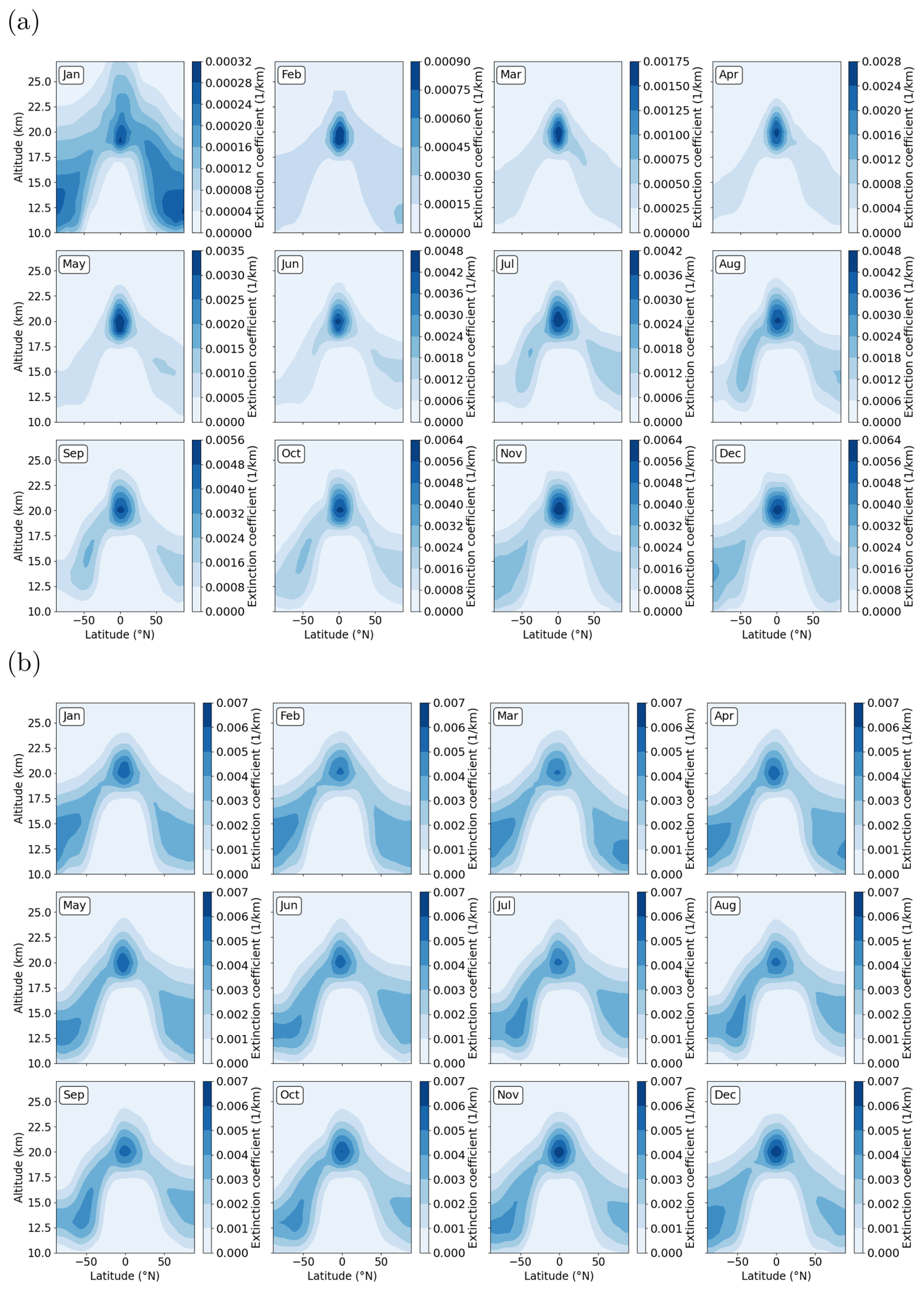
Figure 1 Extinction coefficients at 550 nm for January (Jan) to December (Dec) based on the ECHAM model simulations for the injection of 1 Tg S yr⁻¹. Upper panel (a): results for the initial phase (first year shown). Lower panel (b): results for a quasi-steady-state phase. Note that the values of the colour bars vary between the upper panel (a) and lower panel (b).

3.1 Sensitivity study

In order to answer the question of whether it is possible to detect the sulfate aerosols formed from relatively small sulfur injections of 1 and 2 Tg S yr⁻¹ with the currently active satellite occultation instruments, an error analysis was carried out. The aim is first to estimate the individual errors in aerosol extinction caused by uncertainties or incorrect knowledge of relevant input parameters, e.g. ozone, pressure, temperature (compare Table 3), so that an overall error estimate can then be made. For this purpose, the total ozone column was increased by 2 % , the temperature by 2 K, and the corresponding pressure was adjusted so that the air density remains constant. Besides this, the pressure was increased by 2 %, and the pointing error was taken into account by shifting the tangent height grid upward by 100 m. The corresponding references are listed in Table 3. In addition, the noise error taken from the noise covariance matrix was included in the error analysis.

(e.g. Garane et al., 2019)(e.g. Nowlan et al., 2007; Langland et al., 2008)(e.g. Nowlan et al., 2007; Langland et al., 2008)(e.g. Bramstedt et al., 2012)

Table 3 Reference and modified settings for the sensitivity study.

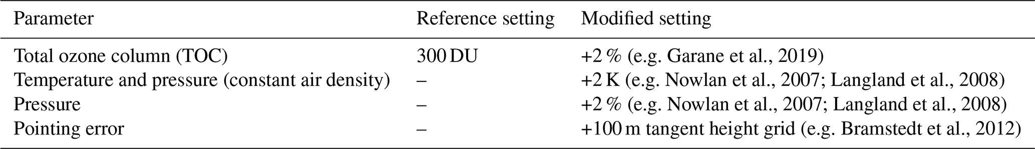
Figure 2 shows the retrieved aerosol extinction profiles at 520 nm with reference settings (black line) and modified settings (red line) exemplarily for 1 Tg S yr⁻¹, 5° N and January based on the ECHAM model simulation results of the quasi-steady-state phase (left column) and the resulting relative difference (individual errors) (right column). The following parameters are exemplarily shown: (a) total ozone column, (b) pressure, and (c) pointing error. More figures for different latitudes can be found in Appendix A (Figs. A2, A3).
The relative differences were determined as follows:

$$\begin{array}{}\text{(6)}& r={\displaystyle \frac{x-\text{ref}}{\text{ref}}}\cdot \mathrm{100}\mathit{\%},\end{array}$$

where ref is the retrieved aerosol extinction profile based on the reference settings (black lines in the left column of Fig. 2), and x the retrieved aerosol extinction profile based on the modified settings (red lines in the left column of Fig. 2).

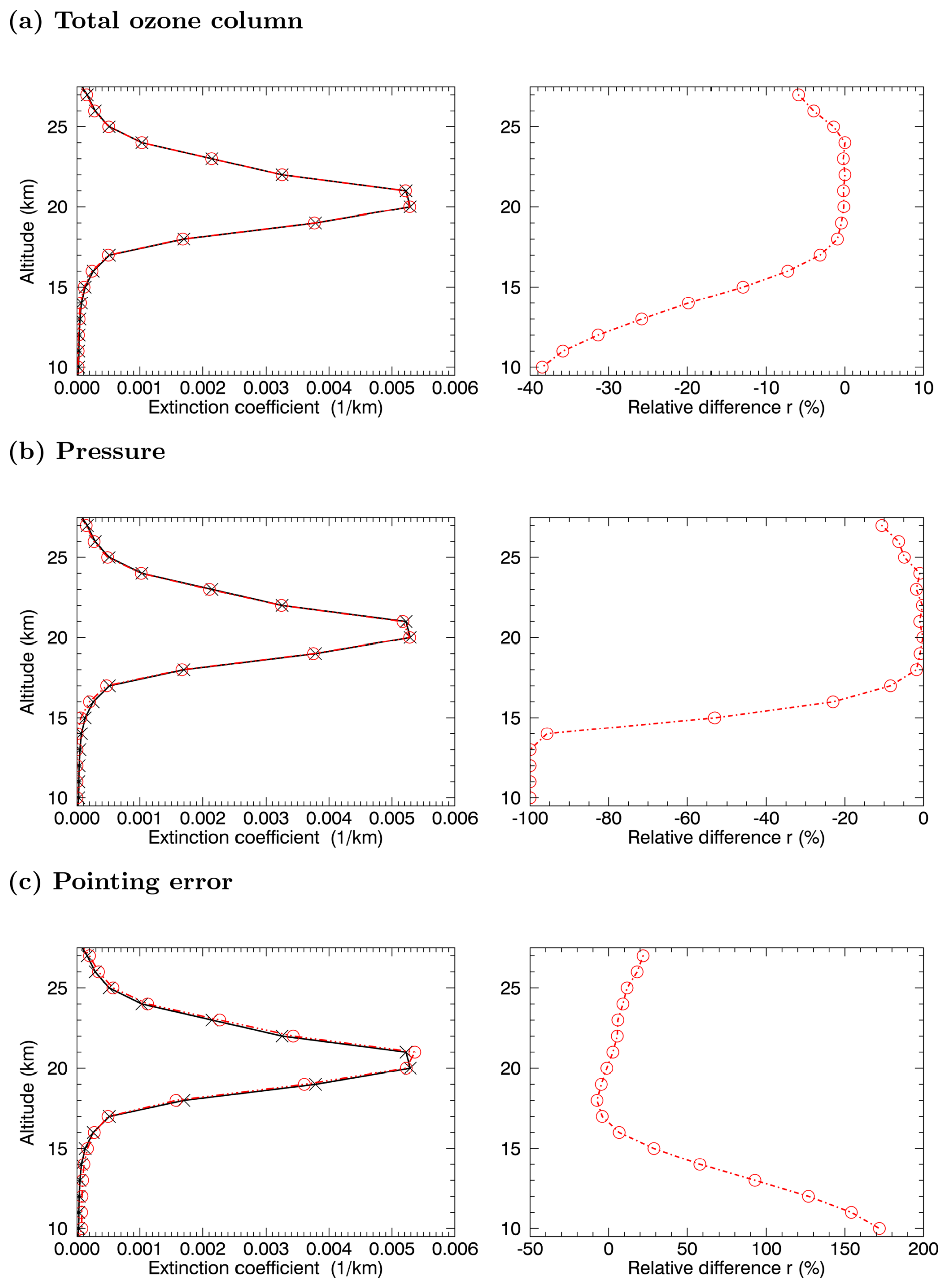
Figure 2 Left column: retrieved aerosol extinction profiles at 520 nm with reference settings (black line) and modified settings (red line) for 1 Tg S yr⁻¹, 5° N latitude and January based on the ECHAM model simulation results of the quasi-steady-state phase. Right column: corresponding relative difference r. Both for perturbed (a) total ozone column, (b) pressure, and (c) shifted tangent height grid.

It should be noted at this point that for the retrievals based on the initial phase data the errors for the background case are used in the following based on the assumption that these errors (relative differences) are larger, which is why an error analysis was also carried out for the background case (explanation below). In order to determine the total error for each height, the subsequent approach was used.

$$\begin{array}{}\text{(7)}& \begin{array}{rl}{\mathit{\sigma }}_{\text{total}}^{\mathrm{2}}& ={\mathit{\sigma }}_{\text{Total ozone column}}^{\mathrm{2}}+{\mathit{\sigma }}_{\text{Temperature}}^{\mathrm{2}}+{\mathit{\sigma }}_{\text{Pressure}}^{\mathrm{2}}\\ & +{\mathit{\sigma }}_{\text{Pointing error}}^{\mathrm{2}}+{\mathit{\sigma }}_{\text{Noise}}^{\mathrm{2}}\end{array}\end{array}$$

The individual errors (relative differences) (compare Eq. 6) of a certain height were added up quadratically. This approach is based on the assumption of random and statistically independent error sources and a linear dependence of the derived aerosol extinction profiles on the parameters. The term “total error” used in the following refers to the square root of Eq. (7).

3.2 Quasi-steady-state phase data

Figure 3 shows the graphical illustration of the total errors in percent (Eq. 7) for 1 Tg S yr⁻¹ (upper panels) and 2 Tg S yr⁻¹ (lower panels), January (left panels), and July (right panels). As described in Sect. 2.1 the quasi-steady-state phase data are an average over 3 years (here years 12 to 15). The total errors at the altitude of the SAI (here 60 hPa ≈ 19 km) depend on the emission rate, month and latitude. For 1 Tg S yr⁻¹, in January it is 10 % (highest value) (85° N) and 3 % (lowest value) (25° N, 25° S, 35° S), and in July it is 47 % (highest value) (85° S) and 3 % (lowest value) (35° S). For 2 Tg S yr⁻¹, in January it is 8 % (highest value) (85° N) and 3 % (lowest value) (25° N, 25° S, 35° S), and in July it is 47 % (highest value) (85° S) and 3 % (lowest value) (35° N, 25° S). Overall, the total errors for 1 Tg S yr⁻¹ are greater than for 2 Tg S yr⁻¹, which is consistent with the expectations, as the signal is stronger at a higher injection rate such as 2 Tg S yr⁻¹, and the total errors are therefore smaller.

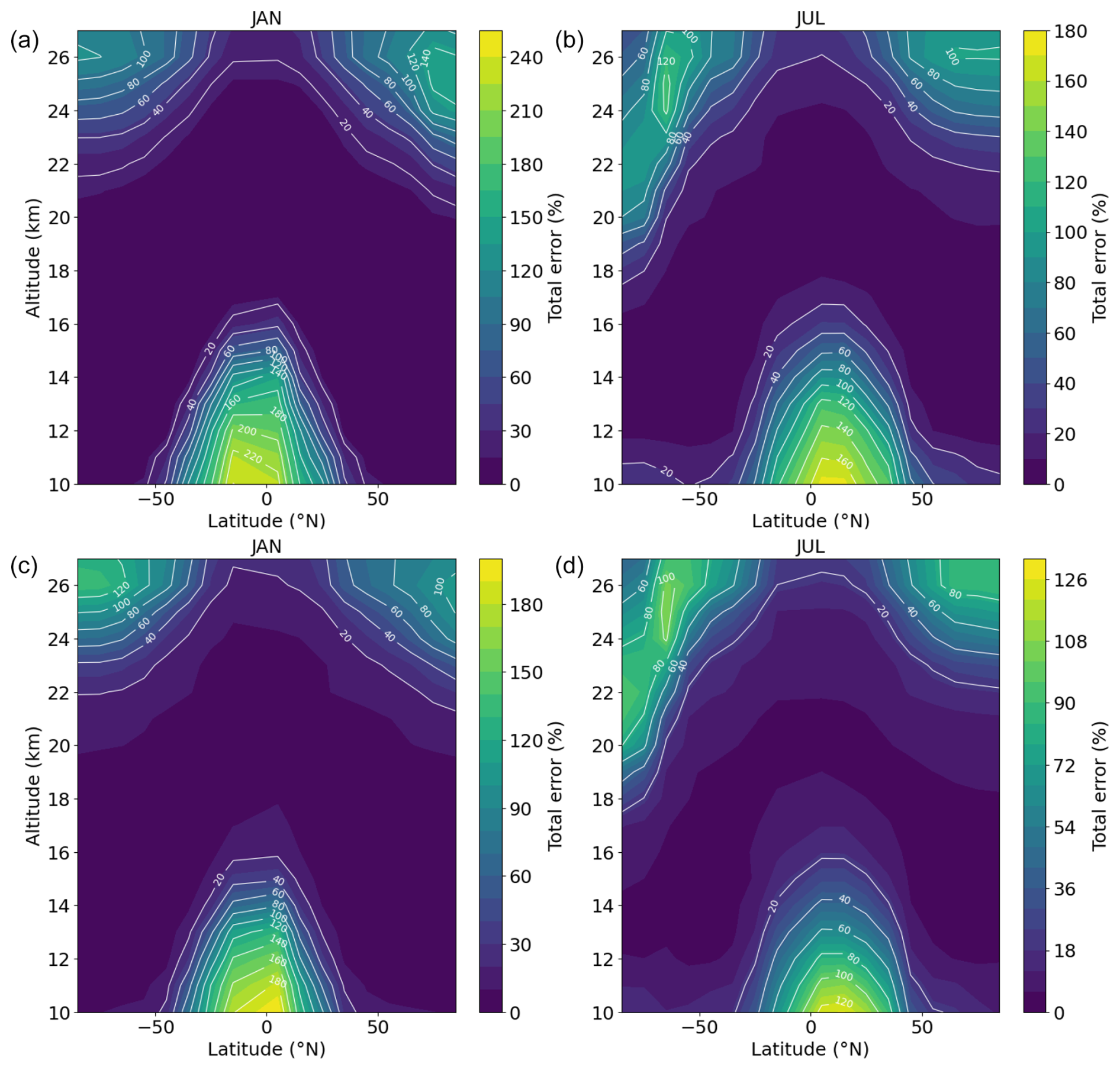
Figure 3 Total errors (%) for 1 Tg S yr⁻¹ (a, b) and 2 Tg S yr⁻¹ (c, d) in January (a, c) and July (b, d) of the quasi-steady-state phase.

Figures 4 and 5 show the retrieved aerosol extinction profiles at 520 nm (black dashed lines) for 1 Tg S yr⁻¹ (Fig. 4) and 2 Tg S yr⁻¹ (Fig. 5), both for January (left column) and July (right column), including the corresponding total errors (red dashed lines), the background profiles (black solid lines), and true profiles (purple solid lines), both at 520 nm (ECHAM model simulation results) for 65° N (upper panels), 15° N (middle panels), and 65° S (lower panels).

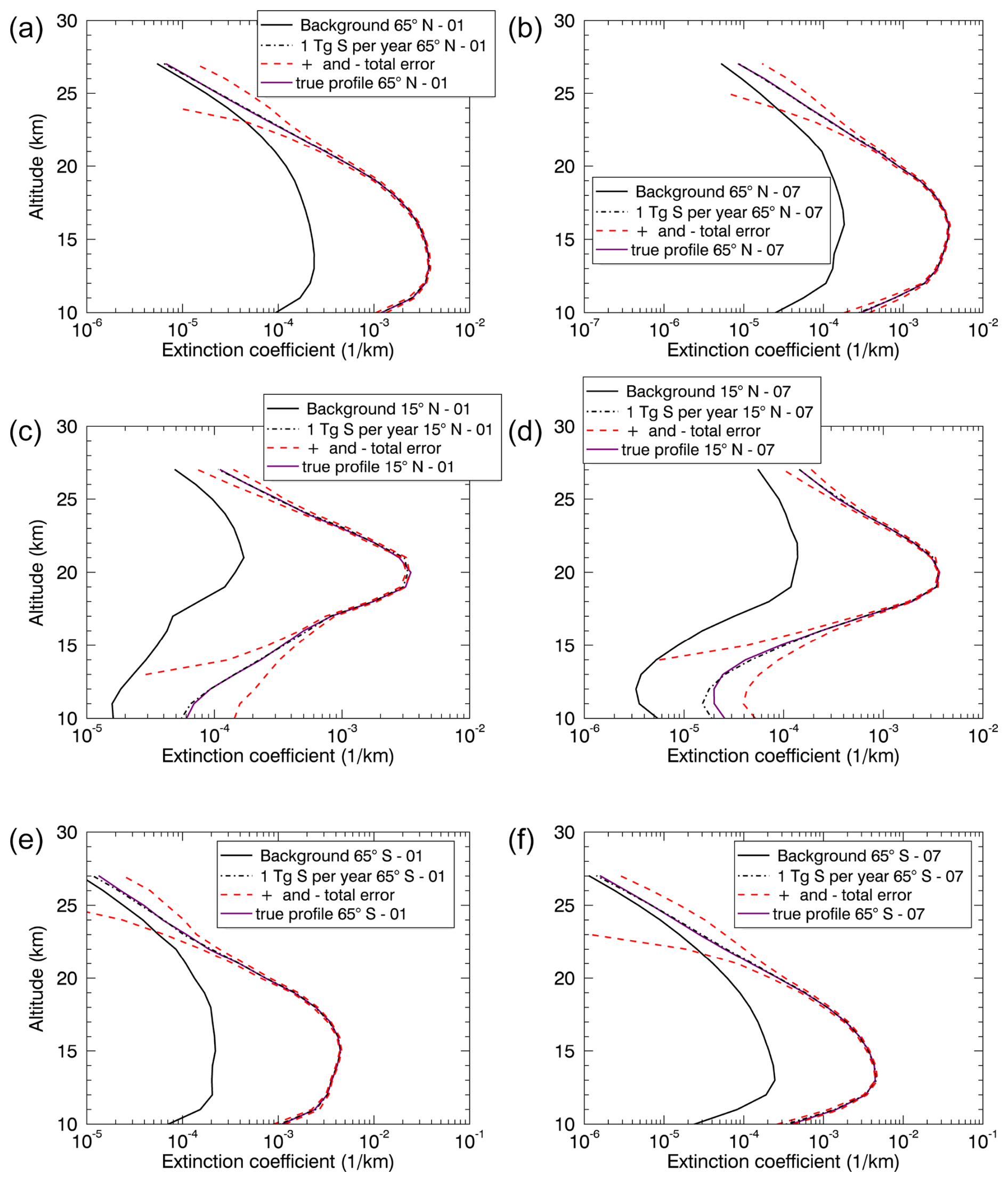
Figure 4 Retrieved aerosol extinction profiles at 520 nm for 1 Tg S yr⁻¹ in January (a, c, e) and July (b, d, f) of the quasi-steady-state phase including total errors, background profiles (520 nm), and true profiles (520 nm) (ECHAM simulation results). Latitudes: 65° N (a, b), 15° N (c, d), and 65° S (e, f).

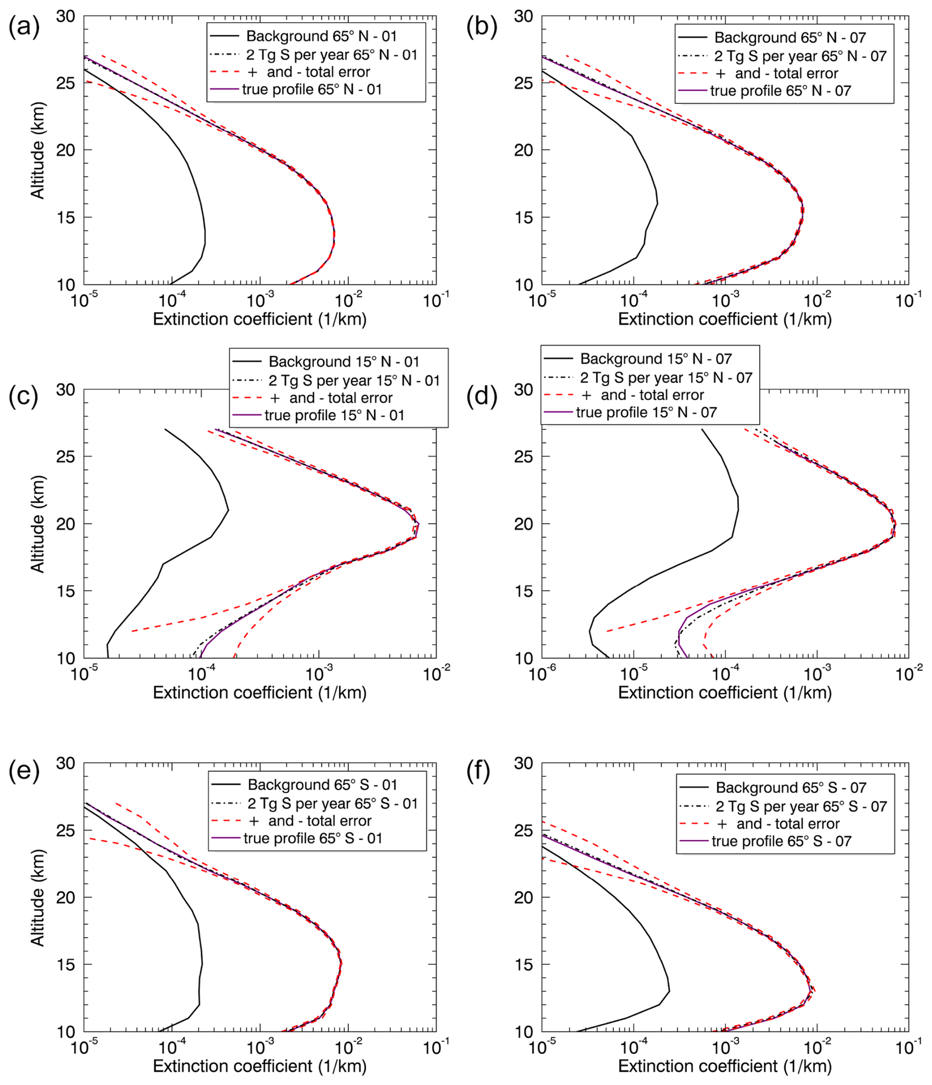
Figure 5 Retrieved aerosol extinction profiles at 520 nm for 2 Tg S yr⁻¹ in January (a, c, e) and July (b, d, f) for the quasi-steady-state phase including total errors, background profiles (520 nm), and true profiles (520 nm) (ECHAM simulation results). Latitudes: 65° N (a, b), 15° N (c, d), and 65° S (e, f).

The basic idea is that the artificial aerosol enhancement is observable in a certain altitude range if the background profile is outside the error range of the extinction profiles of 1 and 2 Tg S yr⁻¹ (red dashed lines in Figs. 4 and 5). This means that the change due to the additional emissions of 1 or 2 Tg S yr⁻¹ is large enough to be distinguishable from the background. For 1 Tg S yr⁻¹ (Fig. 4), this is the case for 65° N in January and July (upper panels) from ≈10–22 km, for 15° N in January and July (middle panels) from ≈14–27 km, and for 65° S in January and July (lower panels) from ≈10–22 km. Note that only a part of the results at different latitudes are shown here, 65° N, 15° N, and 65° S. For 2 Tg S yr⁻¹ (Fig. 5), the artificial aerosol enhancement is observable for 65° N in January and July (upper panels) from 10–24 km, for 15° N in January and July (middle panels) from ≈13–27 km, and for 65° S in January from ≈10–23 km and in July from ≈10–21 km (lower panels). In both cases, i.e. 1 and 2 Tg S yr⁻¹, it is possible to observe these emissions for the latitudes and months shown here. In the following, the stratospheric aerosol optical depth (SAOD) at 520 nm and the corresponding total error were determined. To calculate the SAOD, the latitude-dependent tropopause heights from SAGE II data (2002–2004) for January (2002) and July (2004 – due to the lack of latitude coverage in 2002 and 2003) were used (NASA, 2012), which is why only latitudes from 55° S to 55° N can be shown here. The upper limit remains at 27 km, corresponding to the altitude range of the given aerosol extinction coefficients (see Sect. 2.1). The total error for the SAOD was calculated using Gaussian error propagation. Figure 6 shows results for latitudes from 55° S to 55° N for January (left column) and July (right column), with 1 Tg S yr⁻¹ (upper panels) and 2 Tg S yr⁻¹ (lower panels), including the corresponding total errors, background cases, and true profiles (ECHAM simulation results).

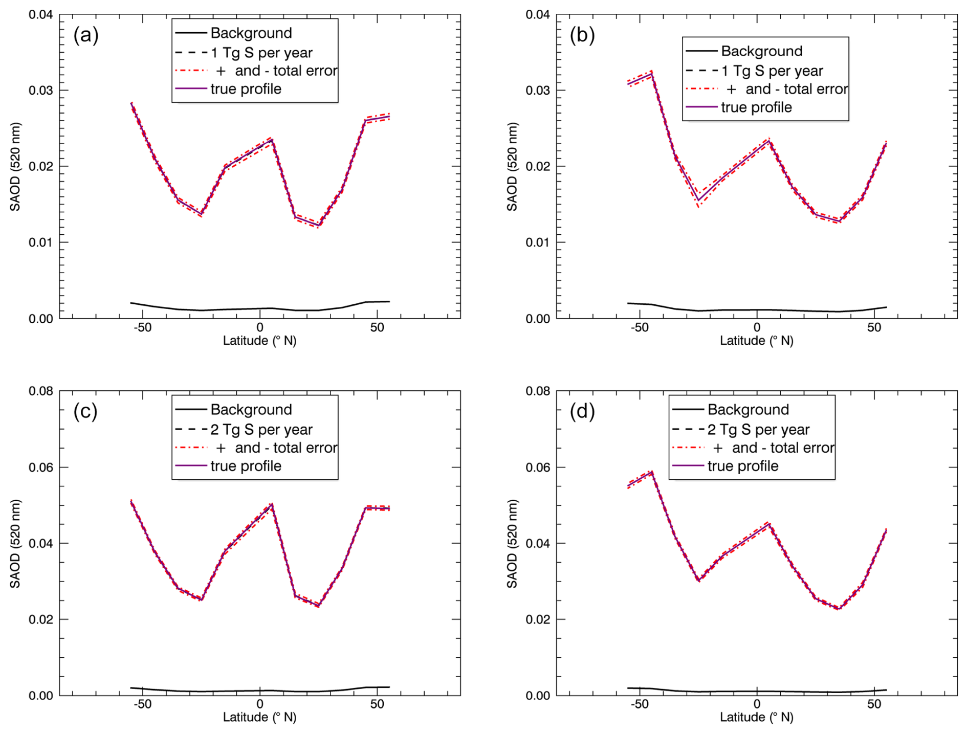
Figure 6 SAOD (520 nm) over latitude (° N) for 1 Tg S yr⁻¹ (a, b) and 2 Tg S yr⁻¹ (c, d), and for January (a, c) and July (b, d), including the corresponding total errors, background cases, and true profiles (ECHAM simulation results).

All subplots show a certain symmetry in the SAOD about the Equator, as well as maxima of the SAOD at mid and high latitudes and minima in the subtropics. The maximum in SAOD near the Equator is due to the fact that 1 or 2 Tg S yr⁻¹ is continuously injected in this region (compare Sect. 2.1). The minima of the SAOD in the subtropics and maxima at mid and high latitudes are due to the latitude dependence of the tropopause height, which is higher in the tropics (about 18 km) than at the mid and high latitudes (about 8 km). Since in all cases, i.e. 1 and 2 Tg S yr⁻¹ for January and July, the background “profile” is outside the error range, it can be concluded that the emissions of 1 and 2 Tg S yr⁻¹ can be observed for the latitudes and months considered here. This means that, under the assumptions made here, it is probably possible to detect the formed stratospheric aerosols with a satellite occultation instrument for the conditions described here. However, it should be noted that the natural variability has not yet been taken into account at this point and will be discussed below.

3.3 Initial phase data

As mentioned above, the total errors from the background case are used for the error analysis of the retrieval of the first month of the initial phase. Figure 7 shows the total errors in percent for the background case, i.e. 0 Tg S yr⁻¹, in January. The aim is to see whether it is possible to observe the emission of 1 Tg S yr⁻¹ in the first month of the initial phase subplot (Jan) of panel (a) in Fig. 1. Comparing the total errors with those for 1 and 2 Tg S yr⁻¹ in the quasi-steady-state phase (see Sect. 3.2), the total errors in the background case are clearly larger. Also in this case, the total errors vary with altitude and latitude (see Fig. 7).

Figure 7 Total errors (%) for 0 Tg S yr⁻¹, i.e. background, and January.

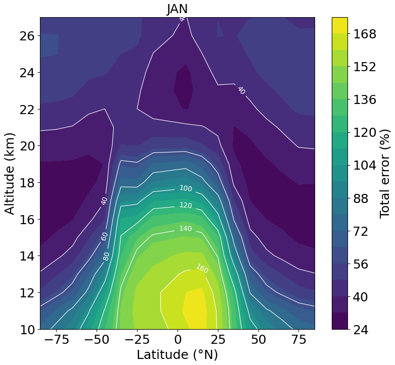
Figure 8 illustrates the SAOD (520 nm) from 55° S to 55° N for 1 Tg S yr⁻¹ in January, including the corresponding total errors, the background case, and the true profile (ECHAM simulation results). Analogous to the quasi-steady-state phase data, the latitude-dependent tropopause heights from SAGE II data were used for the calculation of the SAOD. While for the quasi-steady-state phase data (Fig. 6), the emissions of 1 and 2 Tg S yr⁻¹ in January were observable at all latitudes; this only applies here for $\approx -\mathrm{10}$ to 14° N. However, this is the essential latitude range, since the highest values of the extinction coefficients also occur in this range (Fig. 1, upper panel, subplot (Jan), for 550 nm), and this is also the range in which the SAOD (520 nm) for 1 Tg S yr⁻¹ deviates more clearly from the background case (compare Fig. 8). In addition, Fig. 9 shows the retrieved aerosol extinction profiles at 520 nm for 65° N (upper panel) and 5° N (lower panel), including the total errors, background profiles, and true profiles (both at 520 nm). The background profile for 65° N (upper panel) is within the error range for all altitudes considered here, which leads to the conclusion that the emission of 1 Tg S yr⁻¹ cannot be observed at 65° N in January, i.e. the first month of the initial phase. In contrast, this emission can be observed at 5° N (lower panel) at an altitude of ≈22 km. The apparent difference regarding the conclusion of the detectability of the geoengineering signal between the aerosol extinction profiles (Fig. 9) and the SAOD (Fig. 8) lies in the method for the calculation of the errors of the SAOD, here the Gaussian error propagation, which leads to a reduction of the SAOD errors.

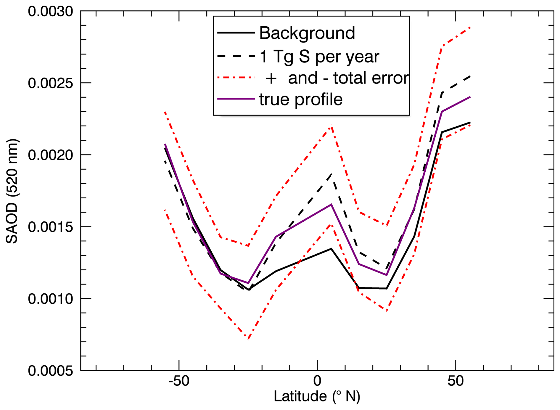
Figure 8 SAOD (520 nm) over latitude (° N) for 1 Tg S yr⁻¹ in January in the first year of the initial phase, including the corresponding total errors, the background case, and the true profile (ECHAM simulation results).

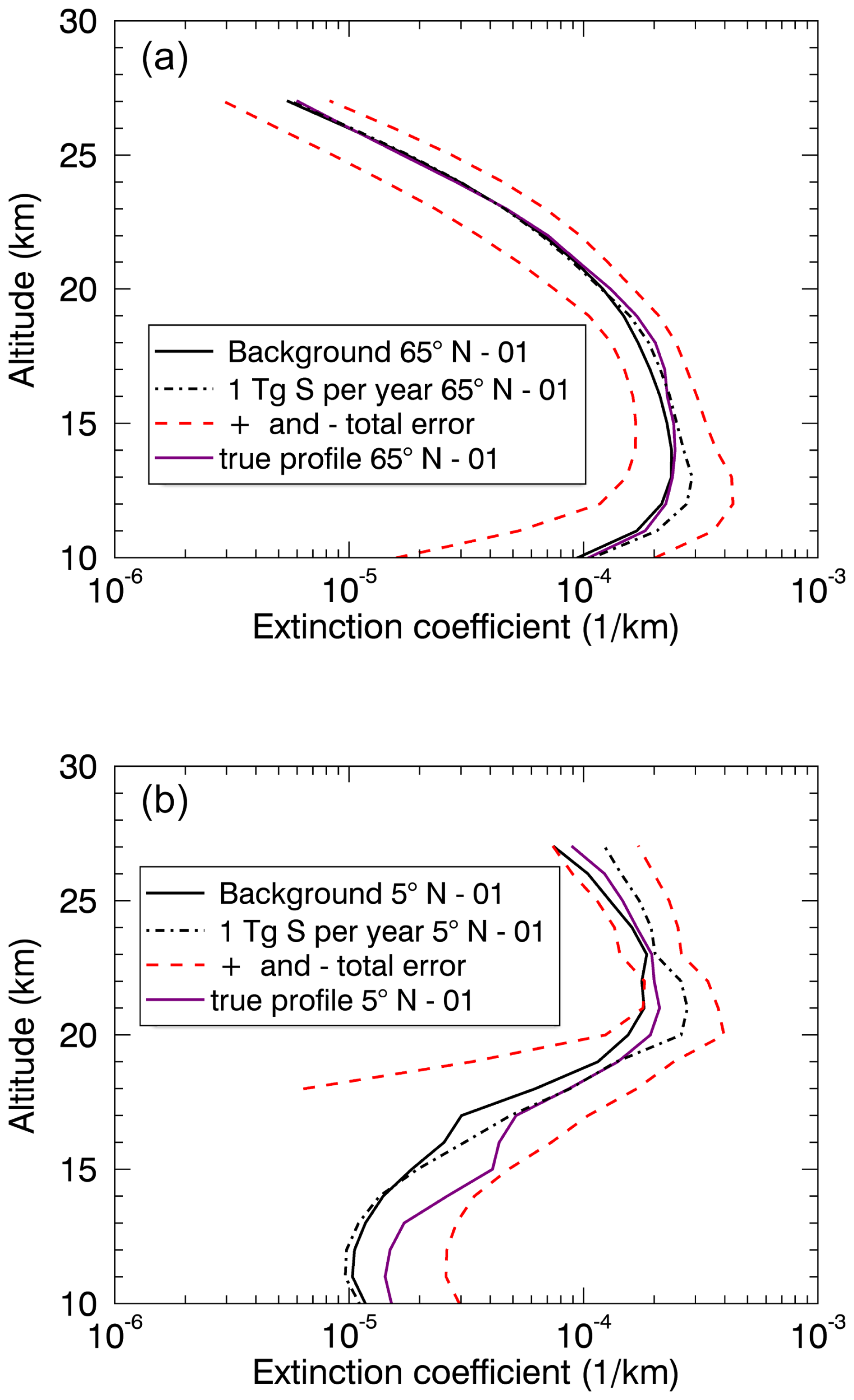
Figure 9 Retrieved aerosol extinction profiles at 520 nm for 1 Tg S yr⁻¹, January, 65° N (a), and 5° N (b), including total errors, background profiles (520 nm), and true profiles (520 nm) (ECHAM simulation results).

In summary, the stratospheric aerosols formed from the emissions of 1 and 2 Tg S yr⁻¹ based on the ECHAM model simulations can be observed for the quasi-steady-state phase under the conditions and constraints considered here (see above). Although 1 and 2 Tg S yr⁻¹ do not have a significant climatic effect, these emission rates were chosen to see whether it is possible to detect even these small amounts with a satellite occultation instrument, taking into account an error estimate that is as realistic as possible. The upper limit of the injection amount depends on the specific goal. Depending on the model, 8 to 16 Tg SO₂ per year would be required to cool the Earth's surface by 1 K on a global average (Niemeier, 2023). We assume that with larger injection rates the detectability increases, the aerosol extinction signal becomes larger, and the total errors become smaller (compare 0 Tg S yr⁻¹ → 1 Tg S yr⁻¹ → 2 Tg S yr⁻¹) up to a certain amount, possibly about 20 Tg (as in the case of the Mt Pinatubo eruption, although a volcanic eruption does not represent continuous injections). However, we note that the zero transmittance problem does not mean that solar occultation measurements are entirely useless. They cannot provide aerosol extinction below a certain altitude, but at slightly higher altitudes they will still work and provide information on enhanced aerosols levels. In the case of Mt Pinatubo, SAGE II measurements were always available at altitudes above about 24 km.

At this point, it should be noted that the relatively large errors at low altitudes (compare Figs. 3 and 7) are due to the low extinction coefficients at these altitudes (compare, for example, Figs. 4 and 5).

Wrana et al. (2021) (Table 1) show the extinction measurement uncertainties at 520 nm averaged from June 2017 to December 2019 at an altitude of 20 km (SAGE III/ISS level 2 solar aerosol product) with a value of 5.66 %. The total errors for 1 and 2 Tg S yr⁻¹ at 20 km are of approximately the same order of magnitude for the northern and southern midlatitudes. Note that it is difficult to make a comparison, as the present study considers different phases (quasi-steady-state phase and initial phase) and different injection rates (1, 2 Tg S yr⁻¹, and background), which means that only a comparison of the order of magnitude is possible.

The measurement frequencies of, for example, SAGE III/ISS averaged over a given month and latitude for the years 2017–2024 are ≈20 measurements for January and ≈30 measurements for July (between 20° S and 20° N). However, the measurement sampling is highly variable and dependent on the month and the respective latitude.

The latitude range investigated here, 85° S–85° N, is wider than that covered by, for example, SAGE III/ISS, but the high latitudes were investigated in order to obtain information on the detectability over the largest possible latitude range. The same applies to the latitudinal coverage (due to the actual sampling issues of occultation measurements).

In the analyses so far, the natural variability has not yet been taken into account, which is of course also crucial for drawing conclusions about the detectability of possible geoengineering experiments.

3.4 Natural variability

In order to evaluate the magnitude of the natural variability of the SAOD under nearly background conditions, SAGE II data from 2002–2004 were used (NASA, 2012). For this purpose, the latitude range 85° S to 85° N (zonal means) and the SAOD at 525 nm were analysed. For different latitudes and months, the mean SAOD and standard deviation were calculated based on the 3-year data. To determine the SAOD, the tropopause heights from the SAGE II data were used. The geoengineering signal is considered detectable if the corresponding SAOD is outside the 2σ range of the natural variability. Figure 10 shows the mean SAOD at 525 nm over the months from January to December for the SAGE II data from 2002–2004, illustrated for 50° S (left panel) and 30° N (right panel). The vertical bars represent the standard deviation of the SAOD values for each month.

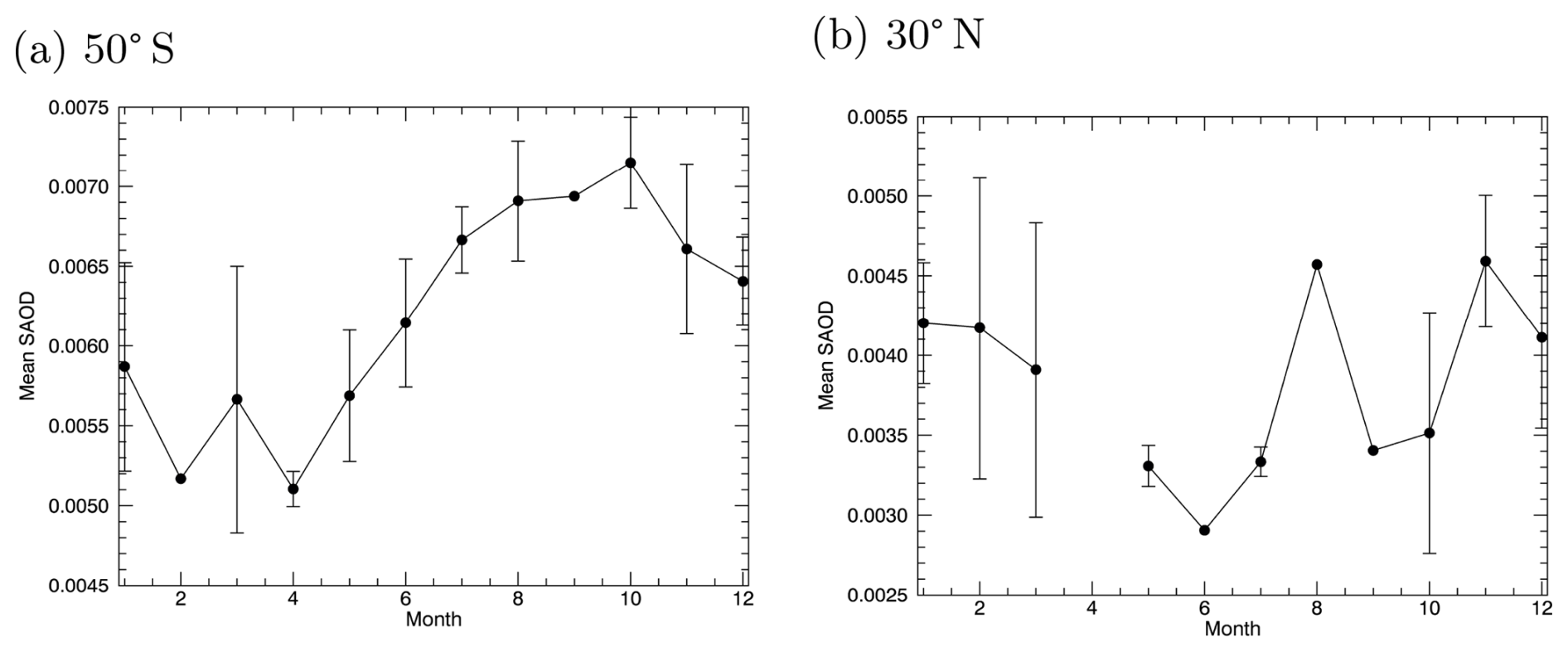
Figure 10 Mean SAOD (525 nm) over month for the SAGE II data from 2002–2004. The vertical bars indicate the standard deviation of the SAOD values for each month. Illustrated for 50° S (a) and 30° N (b).

For the quasi-steady-state phase and the 1 and 2 Tg S yr⁻¹ (e.g, Fig. 6), the SAOD values lie outside the 2σ limit, which corresponds to values of the order of 10⁻³, while the SAOD values themselves are within the 10⁻² range. This means that the emissions, i.e. the stratospheric aerosols formed, can also be detected taking into account a realistic measure of the natural variability. In contrast, the SAOD values in the first month of the initial phase after the 1 Tg S yr⁻¹ injection are within the range of natural variability in the relevant latitude range (compare e.g. Fig. 8), so at this point it is probably not possible to distinguish the geoengineering signal from the natural variability.

The accuracy of the SAGE II/III data, in this case the aerosol extinction coefficients, can also be affected by instrumental and model-related potential error sources. For example, the pointing accuracy, temperature and pressure profiles, correction of atmospheric refraction, and measurement noise (e.g. Damadeo et al., 2013; SAGE III ATBD, 2002).

4 Conclusions

Using the ECHAM simulation results and the radiative transfer model SCIATRAN, it is possible to theoretically answer the question of the detectability of possible geoengineering experiments, here the emissions of 1 and 2 Tg S yr⁻¹, using satellite occultation instruments.

For this, aerosol extinction coefficients at 500 and 550 nm, in an altitude range of 10 to 27 km, simulated with ECHAM, were used to calculate the extinction coefficients at 520 nm applying the Ångström parameterization to simulate transmission values at 520 nm from the perspective of SAGE III/ISS with the radiative transfer model SCIATRAN. These simulated transmission values were then utilized for the retrieval of the stratospheric aerosol profiles with SCIATRAN. A subsequent sensitivity study and error analysis, as well as the consideration of the natural variability using SAGE II data, were applied to answer the question of detectability.

Considering the measurement errors, the natural variability, and the assumptions in the simulations with ECHAM and SCIATRAN, it is very likely that the formed stratospheric aerosols, from the emissions of 1 and 2 Tg S yr⁻¹, can be observed in the quasi-steady-state phase over all latitudes and months considered here.

In the first month of the initial phase, the signal of the emission of 1 Tg S yr⁻¹ cannot be distinguished from the natural variability, which is why the detection of the formed stratospheric aerosols as geoengineering signal is probably not possible. Accordingly, it can be assumed that smaller emission rates cannot be detected as geoengineering signals during the first month of the geoengineering experiment.

Appendix A

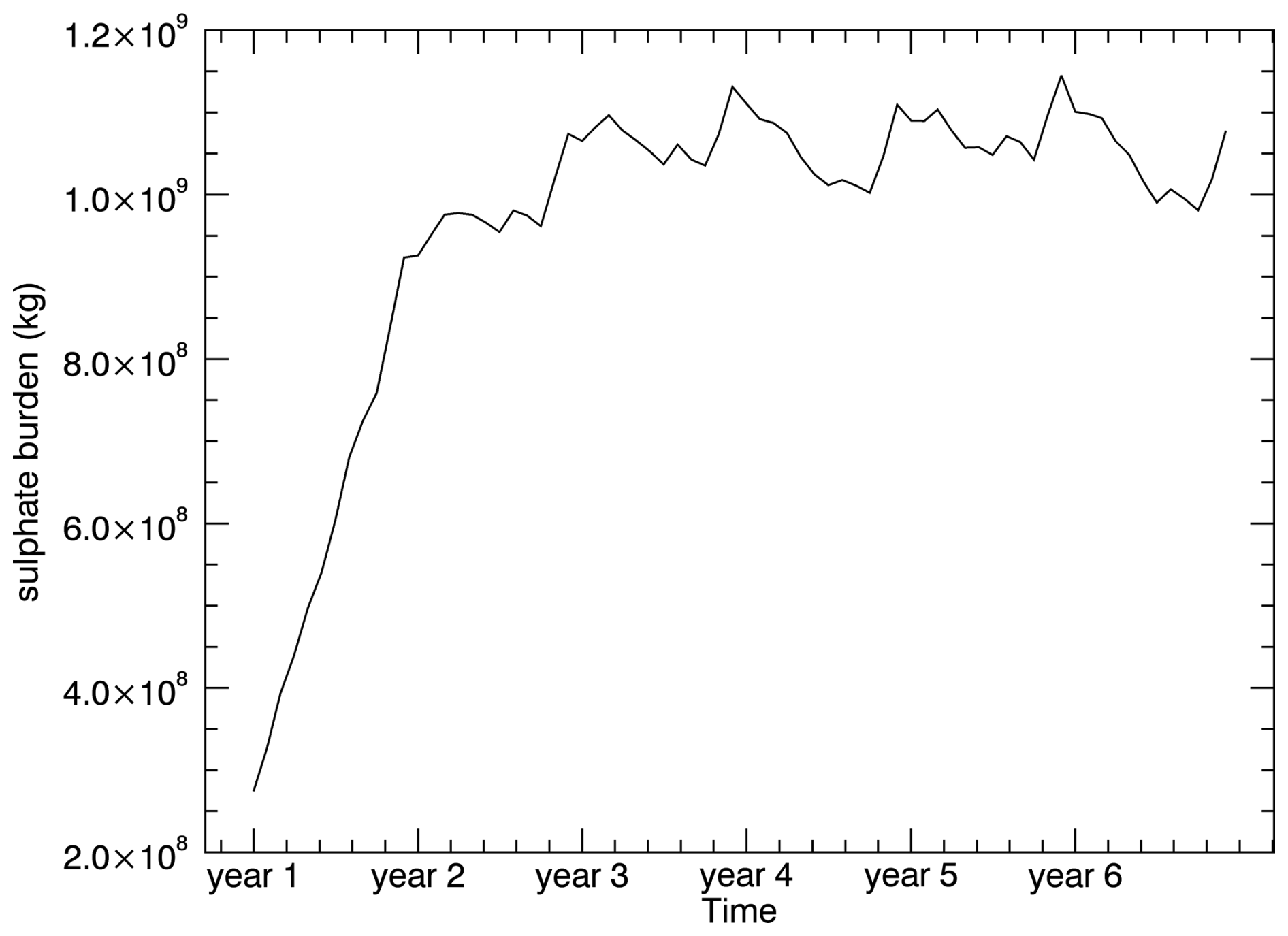
Figure A1 Monthly mean sulfate burden (in kg) over time (2005–2010) for 1 Tg S yr⁻¹, showing the differences between the 2-year initial phase and the quasi-steady-state phase.

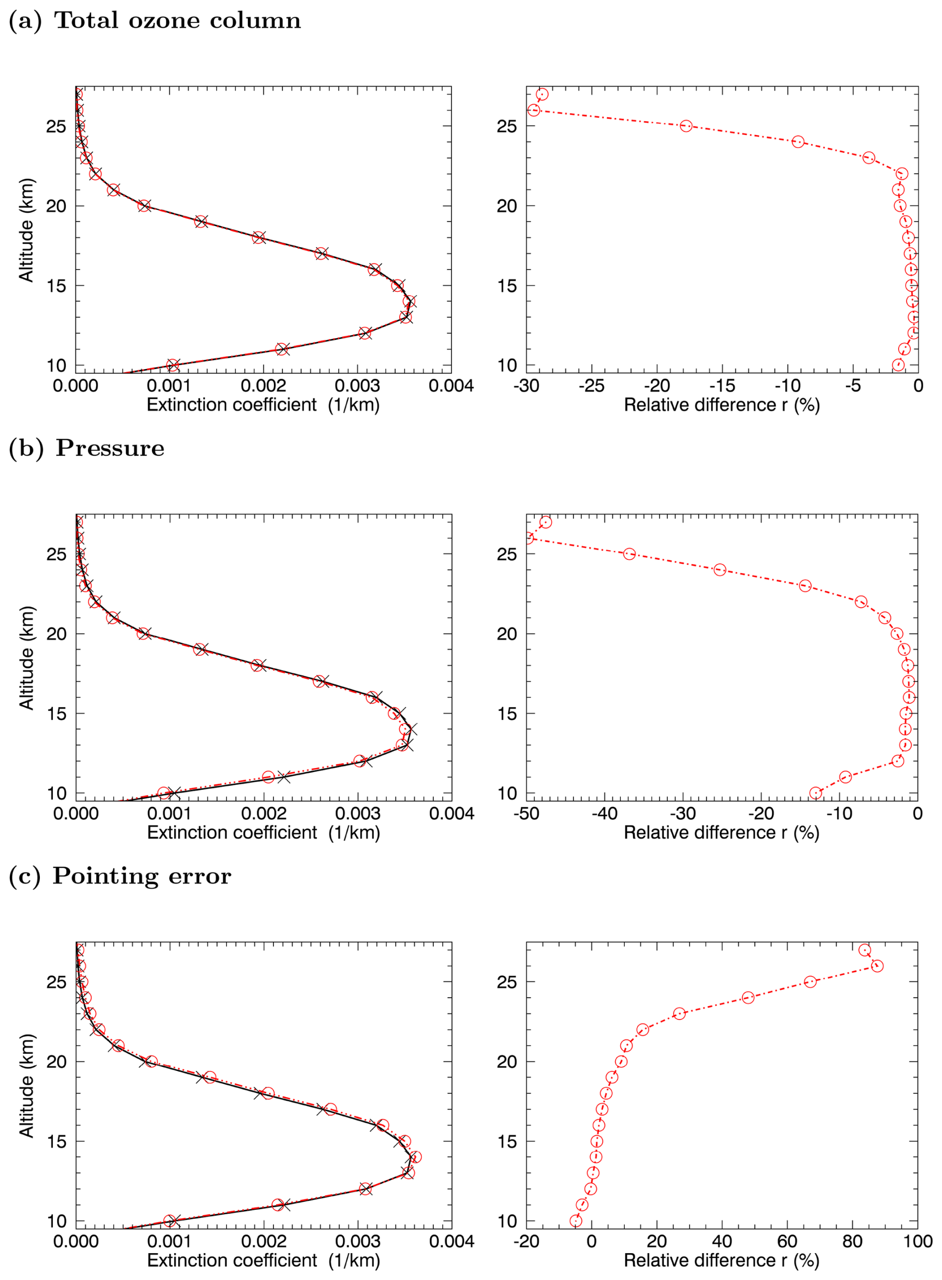
Figure A2 Left column: retrieved aerosol extinction profiles at 520 nm with reference settings (black line) and modified settings (red line) for 1 Tg S yr⁻¹, 55° N latitude, January based on the ECHAM model simulation results of the quasi-steady-state phase. Right column: corresponding relative difference r. Both are for perturbed (a) total ozone column, (b) pressure, and (c) shifted tangent height grid.

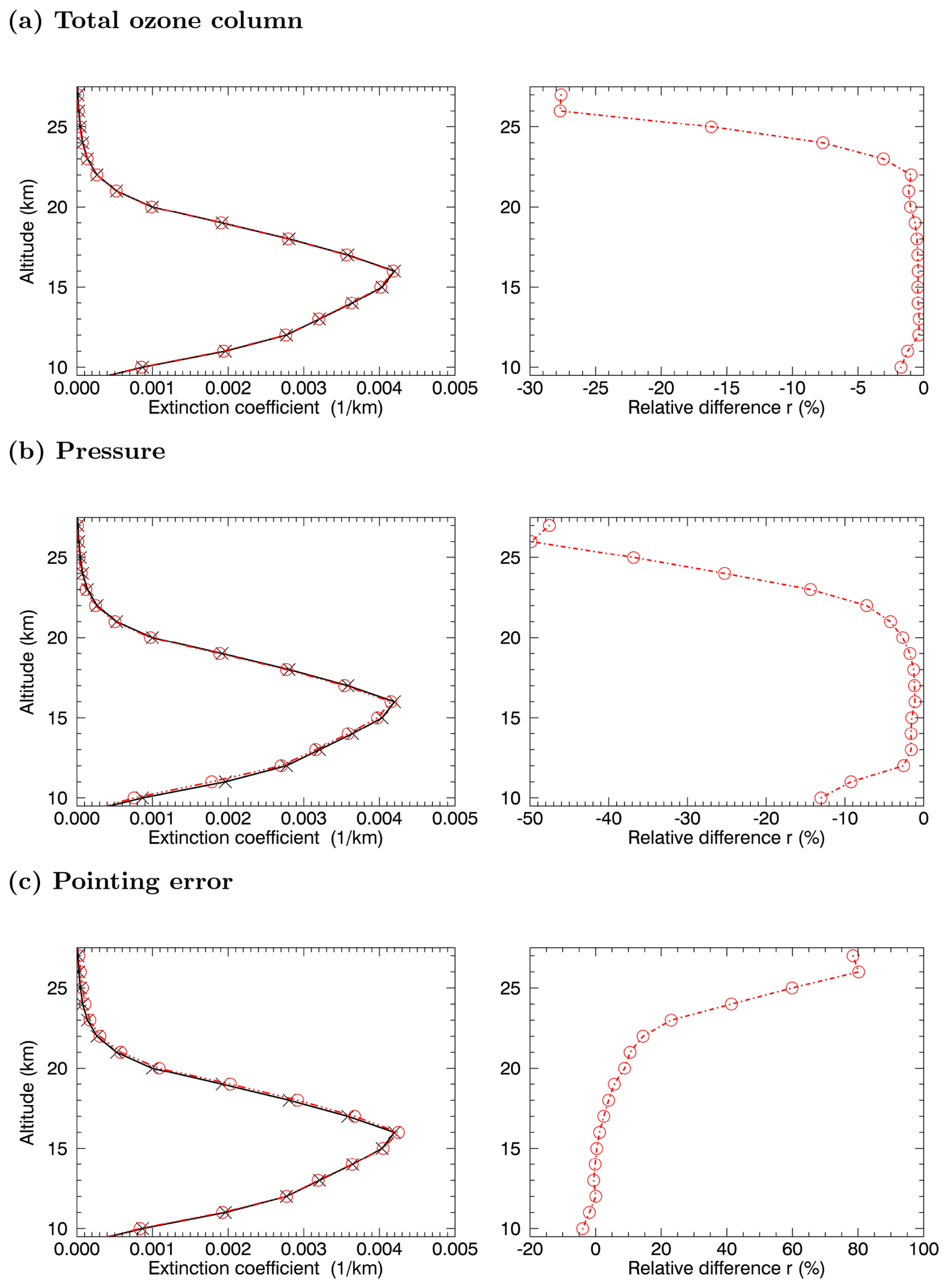
Figure A3 Left column: retrieved aerosol extinction profiles at 520 nm with reference settings (black line) and modified settings (red line) for 1 Tg S yr⁻¹, 55° S latitude, January based on the ECHAM model simulation results of the quasi-steady-state phase. Right column: corresponding relative difference r. Both are for perturbed (a) total ozone column, (b) pressure, and (c) shifted tangent height grid.