the Creative Commons Attribution 4.0 License.
the Creative Commons Attribution 4.0 License.
 | 29 Sep 2025
Quantifying the decay timescale of volcanic sulfur dioxide in the stratosphere
Kane Stone
Susan Solomon
Simon A. Carn
The injection of sulfur dioxide (SO2) into the stratosphere and its subsequent oxidation to form sulfate aerosols after large volcanic eruptions can have profound effects on Earth's climate. The removal of volcanic SO2 in the stratosphere is thought to be driven by its gas-phase oxidation by the hydroxyl radical (OH); once oxidized, it goes on to form sulfate aerosols. However, it has also been suggested that heterogeneous oxidation on ash could also be important or even dominant, which would imply the faster removal of SO2 and thus the faster formation of aerosols, at least in ash-rich plumes. Additionally, recent work uses an assumed exponential fit to determine the total SO2 mass loading following large eruptions; the quality of this fit translates directly to the accuracy of the mass loading estimate. It is therefore of interest to examine how accurately the SO2 decay timescale can be determined from observations and to compare observations to models. Here we evaluate the SO2 decay timescale and its uncertainties following several significant eruptions using three different sets of satellite observations and compare these to the CESM2-WACCM6 model. We show that defining an accurate baseline against which a volcanic injection can be quantified increases the variability and uncertainty in the estimated decay timescale for some satellite datasets. While the typical decay timescale for SO2 is on the order of a few weeks to a month, we find that uncertainties across different altitudes and eruptions result in timescales that can vary by more than a factor of 2. This makes it difficult to attribute variations in the decay timescale to specific SO2-removal processes for the events examined.
- Article
(6010 KB) - Full-text XML
-
Supplement
(620 KB) - BibTeX
- EndNote


The stratospheric aerosol layer is predominantly composed of sulfuric acid and water particles and plays a key role in both atmospheric chemistry and climate. These particles provide surfaces on which the activation of ozone-depleting chlorine takes place, and they can backscatter part of the incoming solar radiation out to space, moderating surface temperatures. Understanding the processes controlling stratospheric aerosol formation and residence times thus hinges on understanding the physical and chemical mechanisms influencing sulfur in the stratosphere. The most important sulfur-containing species for stratospheric aerosol formation is sulfur dioxide (SO2). SO2 is emitted naturally through volcanoes and anthropogenically via the combustion of fossil fuels and the smelting of sulfur-containing metal ore (Pumphrey et al., 2015).
An important source of stratospheric SO2 in non-volcanic conditions is the photolysis of carbonyl sulfide (COS), which is the most abundant sulfur-containing gas in the atmosphere (Kremser et al., 2016). Important sources of COS include its direct flux from the ocean, the oxidation of marine-originating dimethyl sulfide and carbon disulfide, and direct and indirect anthropogenic emissions, among others (Kremser et al., 2016). With a tropospheric lifetime on the order of years (Brasseur and Solomon, 2005), COS can be transported to the stratosphere, where it then photolyzes and ultimately produces SO2. Anthropogenic SO2 can also frequently reach the stratosphere in the tropics via deep convection, especially in the Indian monsoon (Neely et al., 2014).
However, by far the most significant perturbations in stratospheric SO2 are the result of moderate- to large-magnitude volcanic eruptions (volcanic explosivity index (VEI) 3+ and ≥ 1 Tg SO2 emitted) (Solomon et al., 2011; Kremser et al., 2016; Schmidt et al., 2018; Carn et al., 2016). These Plinian-type eruptions feature plumes that entrain and heat ambient air as they rise, enhancing their own buoyancy and enabling them to ascend well above the tropopause (Carey and Bursik, 2015). Once the plume reaches the stratosphere, the SO2 gas is oxidized and forms sulfate aerosols. The gas-phase oxidation process for stratospheric SO2 involves the following reaction sequence (Brasseur and Solomon, 2005):
where the initial oxidation of SO2 by OH is the rate-limiting step. Depending on the environment in which the H2SO4 gas is present, it will either readily be taken up into pre-existing particles (increasing their size) or nucleate along with water vapor to form new particles (Yue, 1981). Once formed, the residence time of stratospheric sulfate aerosols ranges from a few months to a couple of years, depending on the latitude, injection height, and time of year of the eruption. High-latitude eruptions with relatively low injection heights are associated with shorter residence times, whereas the aerosol cloud from tropical eruptions with high injection heights can persist for 1 to 2 years (Toohey et al., 2025; Myhre et al., 2013).
Given the far-reaching impacts of sulfur-derived stratospheric volcanic aerosols on both climate (e.g., McCormick et al., 1995; Robock, 2000; Stenchikov et al., 2009; Schmidt et al., 2018) and ozone (O3) depletion (Solomon et al., 1998), quantifying the amount of SO2 reaching the stratosphere following a major volcanic eruption and its subsequent chemical fate is important (McKeen et al., 1984). In this work, our primary goal is to characterize the decay timescale SO2 following large volcanic eruptions, which reflects the oxidation rate of SO2. Moreover, since the rate-limiting step in the conversion of SO2 to sulfate aerosol is the initial oxidation of SO2, one would expect that the rate of sulfate formation would match the rate of SO2 removal. Thus a better understanding of SO2 removal times also translates to a better understanding of sulfate aerosol formation times, as discussed below.
In addition to understanding the chemical fate of SO2, an exponential fit of the SO2 decay following large eruptions can be used to estimate the total stratospheric SO2 mass burden (Pumphrey et al., 2015; Höpfner et al., 2015). The SO2 mass burden is a key quantity for assessing the climate and chemical impacts of SO2. Here we explain how its accuracy depends on the accuracy of the exponential fit.
Based on the gas-phase oxidation process given in Reactions (R1)–(R3), one would expect that the decay timescale of SO2 increases with height due to the exponential decrease in pressure with height, which limits the rate of Reaction (R1). Indeed, Carn et al. (2016), in their review of satellite measurements of volcanic degassing, show a substantial increase in total-column SO2 e-folding time with injection height, ranging from less than 1 d for those eruptions that do not penetrate the tropopause to upwards of 40 d for the largest eruptions in the last 100 years (see their Fig. 14). However, total column measurements obscure vertical variations in SO2 oxidation rates within the plume of a particular eruption. Höpfner et al. (2015) use vertically resolved observations from the Michelson Interferometer for Passive Atmospheric Sounding (MIPAS) and find that for a given eruption, the SO2 decay timescale generally increases across 10 to 14, 14 to 18, and 18 to 22 km height bins (see their Table 3).
While these observations of the height dependence of the SO2 decay timescale broadly match what we would expect based on Reactions (R1)–(R3), recent work has suggested other possible oxidation mechanisms for SO2 in the stratosphere. Zhu et al. (2020) compared observed total column SO2 decay timescales to model simulations following the 2014 eruption of Kelut in Indonesia. The eruption was notable in part because of a persistent layer of volcanic ash that remained for months after the eruption. They suggest that chemistry involving ash leads to a much shorter timescale of SO2 (17 d when ash is included in their model versus 22–26 d with no ash; see their Table 1). However, Zhu et al. (2020) examined just one volcano, and the timescales they report fall within the range of the values reported by Höpfner et al. (2015). Here we further examine available data on SO2 decay following several different eruptions from different satellites, in part to test the potential role of ash on SO2 oxidation.
Terminology
Before preceding with the rest of the paper, we think it is useful to clarify precisely what we are calculating with respect to the removal of SO2 from the stratosphere. As discussed thoroughly in recent work by Toohey et al. (2025), terms such as “residence time”, “e-folding time”, and “decay timescale” are often taken to be synonymous, when in fact they refer to related but distinct quantities.
Following the discussion in Toohey et al. (2025), consider a tracer injected into a reservoir at time t=0. The mean residence time is the average of the residence times for the tracer particles leaving the reservoir. The e-folding time is the time required for the concentration of the tracer in the reservoir to reach of its initial value. When the removal of the tracer is a purely exponential decay, the residence time will equal the e-folding time. However, both of these quantities can be defined, regardless of the functional form of the decay; for non-exponential decay, they are not necessarily equal.
In this paper, we focus on the “decay timescale” of SO2, which can be defined as follows. Let W(t) be the mass of the tracer in the reservoir after time t=0. The decay timescale τd is defined as
In other words, it is the reciprocal of slope of ln (W(t)) when plotted against time. For a perfectly exponential decay of the tracer mass in the reservoir, the plot of ln (W(t)) versus time will be a straight line, and the slope (the decay timescale) will be equal to both the e-folding time and the mean residence time. However, for non-exponential decay, the decay timescale will vary in time. In practice, we calculate the decay timescale via the slope of a best-fit line to the natural log of SO2 mass. The median decay timescale during the decay period is taken as a measure of the overall behavior and for comparison with other results in the literature. Furthermore, we include a bounds, indicating the spread of decay timescales throughout the decay period. In general, the tighter the bounds, the closer the decay is to exponential. Wider bounds are indicative of increased variability and uncertainty and suggests that a single calculated e-folding time does not sufficiently capture the true nature of the decay. The lack of consensus on this terminology in the literature adds a layer of complication when comparing results. One of our goals here is to draw attention to this potential source of uncertainty.
2.1 Satellite observations
Satellite observations of volcanic SO2 emissions are provided by both nadir-viewing and limb-sounding instruments (e.g., Carn et al., 2016). Nadir measurements using backscattered ultraviolet (UV) radiation (e.g., Sect. 2.1.3) measure the total vertical column density (VCD) of SO2. They provide a good horizontal resolution (∼ 10–50 km) and contiguous global coverage but no vertical resolution. (Vertical profile information can sometimes be derived from UV measurements, but it is computationally expensive and not a standard product.) Nadir observations by infrared (IR) sounders have a similar horizontal resolution and can be used to retrieve SO2 altitude (e.g., Clarisse et al., 2014), but this requires relatively high SO2 column amounts and hence is problematic for dispersed volcanic plumes. In contrast, limb-sounding instruments using emitted microwave and IR radiation (e.g., Sect. 2.1.1 and 2.1.2) provide vertically resolved SO2 profiles (with vertical spacing of ∼ 1.5–3 km) but have a low horizontal resolution (∼ 170 km for MLS and 420 km for MIPAS) and only measure the stratospheric SO2 contribution to the column.
The retrieval of SO2 VCD from nadir UV measurements requires an assumed SO2 vertical profile as input, introducing uncertainty if the assumed profile differs from the actual vertical distribution. However, limb-sounding instruments measure the SO2 vertical profile directly, thus eliminating some of the uncertainty in SO2 mass loading inherent to nadir measurements. Furthermore, because limb-sounding instruments detect emitted radiation from a long horizontal (or tangent) path through the atmosphere, they provide greater sensitivity to volcanic SO2 when the gas is highly dispersed in thin, horizontally extensive layers. Compared to nadir UV measurements, microwave and IR limb sounders also provide higher sensitivity to SO2 at very high latitudes.
Nadir observations are therefore optimal for measuring SO2 mass loading in recently erupted volcanic SO2 plumes (within hours to a few days after eruption), which are relatively compact and poorly sampled by limb sounders. However, once the SO2 becomes dispersed in the atmosphere, the greater sensitivity of limb sounders is advantageous for monitoring the decay of stratospheric SO2, especially at high latitudes. Eruptions at mid- to high latitudes typically experience stronger wind shear than tropical eruptions (e.g., due to interaction with the polar jet stream) and hence may have a tendency to disperse more quickly below the detection limit of nadir instruments.
Here, we focus on data from two limb-sounding instruments (Sect. 2.1.1 and 2.1.2) and one nadir instrument (Sect. 2.1.3). These instruments are discussed in more detail in the following sections.
2.1.1 MIPAS
The Michelson Interferometer for Passive Atmospheric Sounding (MIPAS) instrument was an atmospheric limb sounder that measured radiation in the region of 685–2410 cm−1 via a Fourier transform spectrometer (Fischer et al., 2008). The instrument was on the polar-orbiting satellite Envisat and operated from 1 March 2002 until 8 April 2012. During the time period of the retrievals used in this work, the spectral resolution was 0.0625 cm−1, the horizontal resolution was 420 km, and the vertical resolution was approximately 1.5 km (Höpfner et al., 2015). We accessed the data at https://www.imk-asf.kit.edu/english/308.php (last access: 20 May 2024) and used the reduced spectral resolution version of the data (which is valid from 2005 to 2012). In addition to the SO2 volume mixing ratio, we use retrieved pressure and temperature to convert the volume mixing ratio to mass, as described in later sections. As suggested in the MIPAS data files, we select valid data by using only points where visibility =1 and akm_diagonal >0.03.
2.1.2 MLS
The Microwave Limb Sounder (MLS) is an instrument on NASA's Aura satellite, which launched in July 2004 and has a sun-synchronous orbit (Waters et al., 2006; Schoeberl et al., 2006). The instrument measures thermal emission in the microwave from Earth's limb and has done so with little interruption from August 2004 to the time of writing (Pumphrey et al., 2015). The retrievals of temperature and SO2 mixing ratios used in this work are reported on pressure levels with an approximate spacing of 3 km, and the horizontal resolution is approximately 170 km (Livesey et al., 2022). We use the level 2, version 5 (V5) daily swath SO2 mixing ratio data, accessed at https://disc.gsfc.nasa.gov/datasets/ML2SO2_005/summary?keywords=so2 (last access: 20 May 2024) (Read and Livesey, 2021). The V5 data feature minor changes from previous versions, including improved cloud detection, changes in the calculation of O3 and carbon monoxide (stated to have secondary impacts on SO2), and updates to the handling of background radiance signals (Livesey et al., 2022). These data are obtained via the 240 GHz radiometer on the MLS instrument (Pumphrey et al., 2015). In addition to the SO2 mixing ratio, this dataset reports the temperature at each pressure level, and we use this in our calculation of SO2 mass and altitude above sea level.
The MLS documentation highlights the fact that the retrieval algorithm can generate negative mixing ratios, and the correct way to deal with these is to average over a sufficiently large horizontal area (Livesey et al., 2022). We apply all of the suggested masking for the data given in Livesey et al. (2022), and we average our data over 10° latitude bands. Even after masking and averaging, negative mixing ratios are prominent in the MLS data, particularly lower in the atmosphere.
2.1.3 OMI
Like MLS, the Ozone Monitoring Instrument (OMI) is also on NASA's Aura satellite. With only minor gaps since August 2004, OMI measures ultraviolet and visible nadir solar backscatter (Levelt et al., 2006) and thus does not provide a high-resolution vertical resolution for SO2. Here we use the level 2, version 3 stratospheric estimate of SO2 VCD (Li et al., 2020). These estimates of VCD are reported in the variable ColumnAmountSO2_STL from the OMI product and are given in Dobson units ( ). We follow the guidelines for flagging erroneous values given in the documentation for the dataset (see Li et al., 2020). OMI's stratospheric estimate of VCD is derived using an assumed lower-stratospheric SO2 profile with a center of mass at 18 km. Note that results using the OMI output in ColumnAmountSO2_TRU, which assumes a center of mass at 13 km, had little impact on our results. See Li et al. (2017) for more details on the retrieval algorithm.
2.2 Model data
We compare the satellite data to model output from the Whole Atmosphere Community Climate Model version 6 (WACCM6), which is a component of the Community Earth System Model version 2 (CESM2). Data for 1980–2014, which we use here, were initially published in Gettelman et al. (2019). See this paper for a thorough overview of the details of the model. Throughout the paper, we refer to the model output simply as WACCM.
The horizontal resolution of the model is 1.9° latitude by 2.5° longitude. There are 88 levels in the vertical, extending up to approximately 140 km above the surface of the Earth. The vertical resolution in the upper troposphere and stratosphere is 1–2 km. All major volcanic eruptions from 1980 to 2014 are included in the model. The chemical mechanism includes a detailed representation of stratospheric chemistry, and importantly, the oxidation of stratospheric SO2 is driven by the gas-phase reaction with OH only. Thus, the model provides a useful baseline for determining other potential oxidation pathways in the observations.
2.3 Calculation of SO2 mass
The method used to calculate the SO2 stratospheric burden depends on the units of the initial SO2 data. When starting with the SO2 volume mixing ratio (as is the case for MIPAS, MLS, and the WACCM data), we first convert the volume mixing ratio to a mass mixing ratio using the molar masses of SO2 and air. For every vertical profile, pressure and temperature from the respective product are then used to calculate the air density at each pressure level (using the ideal gas law). Multiplying the air density with the mass mixing ratio yields the density of SO2 at each pressure level.
The MIPAS data are reported on an altitude coordinate with a spacing of 1 km (between 10 and 22 km), and the MLS and WACCM data are reported on a pressure coordinate. In order to compare the datasets, we interpolate the MLS and WACCM data to the altitude coordinate from MIPAS.
For the MLS data, this is done in several steps. At every vertical profile, we first calculate the change in altitude Δzi between successive points pi and pi+1 on the MLS pressure coordinate using hydrostatic balance:
In practice, we evaluate this integral discretely and assume that the density ρair varies linearly from ρair(pi) to ρair(pi+1). The maximum value in the MLS pressure coordinate is 1000 hPa. By assuming that this pressure corresponds to an altitude of 0 km, we can use Eq. (2) to calculate the altitude of every pressure level of every vertical profile in MLS. With this, we then linearly interpolate each vertical profile from MLS to the altitude coordinate of the MIPAS data.
For the WACCM data, the model output geopotential height is used for the interpolation to the MIPAS height grid.
Once the data are on an altitude vertical coordinate, we integrate in the vertical and horizontal to get the total mass of SO2. As we are interested in the oxidation of SO2 as a function of height, we group our data into three height bins used by Höpfner et al. (2015) (10–14, 14–18, and 18–22 km) and vertically integrate in each height bin. We also calculate the total SO2 mass in the upper troposphere/lower stratosphere by integrating from 10 to 22 km. Given the variation in tropopause height with latitude, the 10 to 14 and 14 to 18 km layers will not necessarily be entirely in the stratosphere in low latitudes (Hoffmann and Spang, 2022). However, we use the vertical divisions here for consistency with past work, and future work could consider a vertical division based on tropopause height.
Following Höpfner et al. (2015), for the horizontal integration, we group our data into 10° latitude bands, take the mean of the vertically integrated SO2 data falling in each band, and multiply by the area of the respective latitude band. We perform this calculation for each of the three height bins to find the mass of SO2 in each height bin within each latitude band. Finally, for each height bin, we sum up the mass of SO2 in all of the latitude bands that were clearly affected by the volcanic eruption.
The SO2 mass from OMI is calculated by horizontally integrating the reported vertical column density values. The horizontal integration is the same as that described for the MLS and MIPAS data.
2.4 Calculation of the decay timescale
We determine the decay timescale by first calculating the perturbation due to the eruption from a background SO2 level that occurs in the absence of any volcanic influence. We determine the background for each height bin and 10° latitude band. The time period that defines the non-volcanic background varies by eruption and product, but in general, we select a background such that the SO2 perturbation decays to 0 given enough time. For some eruptions and products, care needs to be taken to select an appropriate background; for example, there is a signal from the eruption of Okmok in the MIPAS data prior to the Kasatochi eruption, and thus we select a background period long after the influence of either eruption is seen in the time series (see Fig. 3f). For the MLS data, we also remove the apparent seasonal cycle for each height bin (if the cycle is present; see Sect. 4.2 for more details on how we remove the seasonal cycle and the implications of doing so).
Once the volcanic SO2 perturbation is isolated, we then determine the decay timescale by fitting a best-fit line of the form (using the notation of Höpfner et al., 2015):
where is the mass of SO2 in height bin Δhi, is the decay timescale in that bin, and t0 is the start of the window used for the calculation. Volcanic plumes can have strong impacts on the local chemical environment in the stratosphere by, for example, altering OH concentrations (especially for high SO2 concentrations), photolysis rates, and water vapor content (McKeen et al., 1984; Carn et al., 2022; Glaze et al., 1997). These impacts can in turn influence the oxidation rate of SO2 and in particular lead to variations in the decay timescale during the decay of the SO2 burden. Thus, in order to assess this potential variability, we perform the calculation over a series of moving windows in time. We use windows of three lengths: 15, 20, and 25 d. For each window length, the calculation is repeated for five different windows, with the first day in each window spaced 5 d apart. The start of the first window coincides with when the SO2 mass begins to decline. When the SO2 perturbation decays in a period shorter than five windows, we adjust the number of windows appropriately. Figure 1 illustrates the way in which the windows are varied to calculate the decay timescale.
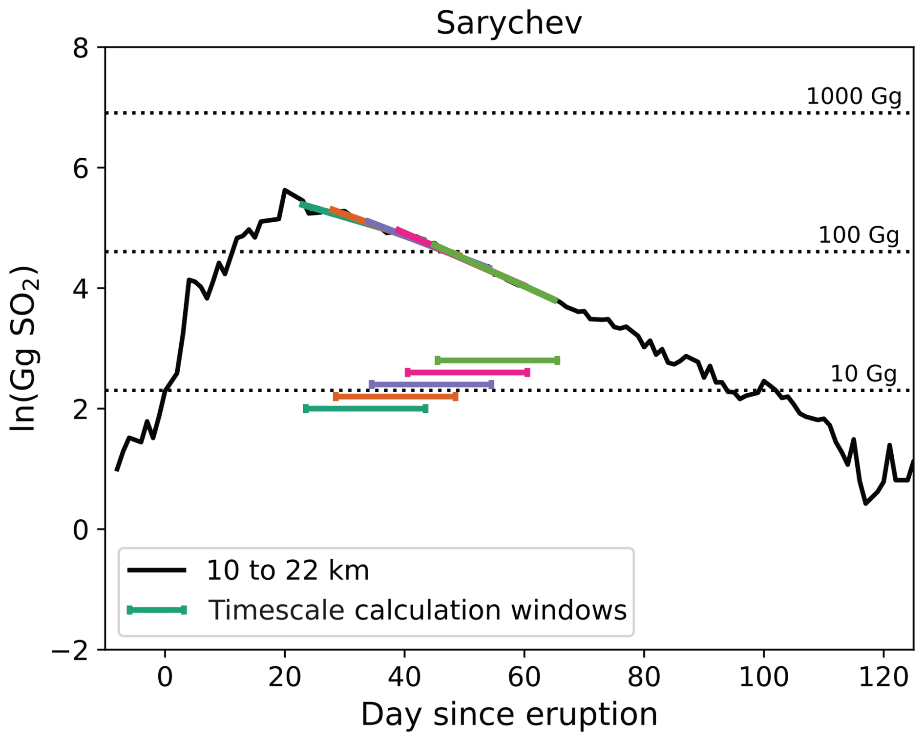
Figure 1 Visual example of the windows used to calculate the decay timescale throughout the decay period. This plot shows the SO2 mass after the 2009 Sarychev eruption between 10 and 22 km from MIPAS (solid black line). The colored lines are linear fits of the curve during different periods of the decay, as indicated by the horizontal line of the same color below the black curve. The window length in this example is 20 d.
The decay timescales collected from all the windows (all lengths and times) give a sense of the total variability of the oxidation rate of the volcanic SO2. The median and 5th and 95th percentiles are used to quantify the spread. Note that we use the median, as opposed to the mean, to limit the influence of the tail towards long timescales.
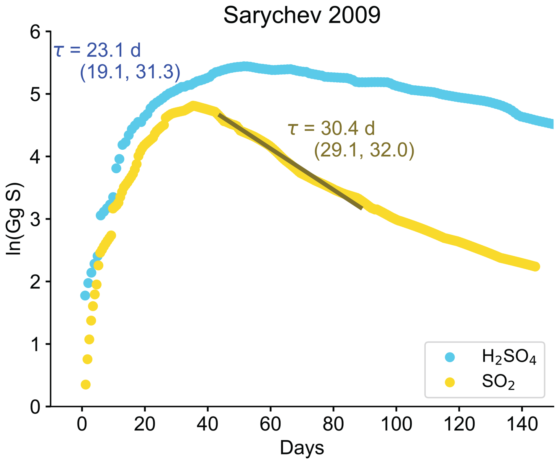
Figure 2 Comparison of SO2 decay timescales and sulfate formation timescales. Data are from Günther et al. (2018) and are retrieved from MIPAS. Masses shown are the total mass from 10.5 to 22.5 km. The timescale of sulfate formation is comparable to that of SO2 removal. Note that time series here are in units of Gg sulfur (as opposed to Gg SO2 used in other plots in the paper). Values in parentheses denote the 5th and 95th percentiles.
The oxidation and subsequent removal of stratospheric SO2 is directly related to the formation of climate- and chemistry-altering sulfate aerosols. Thus, a central underlying motivation for this work is that better quantification of the SO2 removal process directly translates to a deeper understanding of aerosol formation. Before proceeding with the rest of the analysis, we present a simple comparison between the timescale of SO2 removal (which is determined by the oxidation rate) and the timescale of sulfate aerosol formation for the 2009 Sarychev eruption (Fig. 2). We assume the following.
-
The sulfate aerosol perturbation is entirely the result of chemical conversion from SO2.
-
The timescale of sulfate aerosol removal is significantly greater than that of sulfate aerosol formation.
-
The loss of SO2 (and subsequent conversion to sulfate aerosol) is a first-order reaction with timescale τ.
Consequently, the growth of the sulfur mass contained in the sulfate aerosol (mS,aero) is given by
where M0 is a constant and is the mass of sulfur contained in SO2. Solving for mS,aero as a function of time gives
Here, M0 is taken to be the observed peak in the sulfur mass contained in the sulfate aerosol.
Using sulfate data from Günther et al. (2018), we estimate the timescale τ using Eq. (5). We subtract the observed time series of sulfur mass contained in sulfate from its observed maximum. We then take the natural log of the resulting curve and use a linear fit to estimate τ. This fit is done between the start of the eruption and the peak in the sulfate sulfur mass. By varying the window used for this fit, we obtain the 5th and 95th percentiles for the timescale as a confidence interval around the median.
We compare this timescale derived from sulfate formation to that derived from a linear fit to the natural log of the mass of sulfur contained in SO2. The two median timescales are reasonably similar (23.1 versus 30.4 d), and there is some overlap between the 5th and 95th percentile ranges, which gives confidence to the notion that a better understanding of volcanic SO2 decay timescales will improve our understanding of sulfate aerosol formation.
The decay time estimate obtained from Eq. (5) is an approximation and will be sensitive to the instrument's ability to measure sulfate aerosol (see Günther et al., 2018 for a further discussion on the sulfate retrieval). Furthermore, once the sulfate aerosol is formed, it will be removed via sedimentation and transported by the large-scale circulation (e.g., the Brewer–Dobson circulation). Generally these processes are much slower than the timescale for sulfate production (which motivates assumption 2 above). Nonetheless, they may influence the shape of sulfate perturbation (the blue scatter points in Fig. 2) and the subsequent timescale estimate. For a more thorough discussion of the different timescales involved in sulfate aerosol formation and residence time, see Toohey et al. (2025).
4.1 Comparing MIPAS and MLS
We use vertically resolved retrievals of SO2 from two limb-sounding products: the Microwave Limb Sounder (MLS) and the Michelson Interferometer for Passive Atmospheric Sounding (MIPAS) (see Sect. 2 for more details). Both instruments have high temporal and near-global coverage, making their observations suitable for assessing the decay of SO2 both vertically and horizontally as the volcanic plume is mixed and dispersed following the eruption (Höpfner et al., 2015). While past work has analyzed SO2 retrievals in each product individually (for MLS, see Pumphrey et al., 2015; for MIPAS, see Höpfner et al., 2015 and Günther et al., 2018), to our knowledge this is the first direct comparison of their vertically resolved SO2 measurements. The Aura satellite, which carries the MLS instrument, is expected to last until 2028, while MIPAS operated from 2002 through 2012. We focus our analysis on large (greater than 1 Tg SO2 emitted; Carn et al., 2016) eruptions covered by both instruments.
Figure 3 shows the observations from MLS and MIPAS from 2008. While there were a few smaller eruptions in that year, by far the most significant was the eruption of Kasatochi on 7 August 2008 (set to day 0 in the figure and indicated with a vertical dashed line). An island volcano in the Aleutian Islands (52.12° N, 175.51° W), Kasatochi injected an estimated 2 Tg SO2 into the atmosphere, with the plume reaching a height of 15 km (Carn, 2025). Panels (a)–(b) in Fig. 3 show the SO2 daily mean volume mixing ratio (in ppb) in the lower stratosphere as a function of time and latitude, retrieved from MLS (panel a) and MIPAS (panel b). MLS data are reported on a pressure vertical coordinate, whereas MIPAS has altitude as the vertical coordinate. The data plotted in Fig. 3a and b show the daily mean volume mixing ratio at a similar distance above the surface of the Earth prior to any sort of interpolation or integration. This highlights the inherent differences in the underlying data between the two products. While the eruption is clearly visible in both datasets, as indicated by the elevated SO2 shortly after the eruption (day 0), the mixing ratios reported by MLS are negative for much of the year, whereas in MIPAS they are positive and much closer to 0 (compare Fig. 3a to b). Negative mixing ratios are unphysical and an artifact of the MLS retrieval algorithm; nonetheless, the MLS documentation recommends including them in subsequent calculations (Livesey et al., 2022). However, aggregating these negative mixing ratios over a large geographic area (e.g., 40 to 90° N) and converting to mass results in large negative values that complicate the interpretation of the data but are nonetheless included here.
Figure 3c and d show the total SO2 mass between 40 and 90° N for three different height bins: 10 to 14, 14 to 18, and 18 to 22 km (see Sect. 2.3 for more details). We choose these bins to be consistent with those used in Höpfner et al. (2015). While the Kasatochi eruption is clearly visible in Fig. 3c, the MLS data in the 10 to 14 km bin show large negative masses throughout the year. Additionally, the MLS mass in the 10 to 14 and 14 to 18 km bins feature a seasonal cycle with an amplitude much larger than what is expected for background stratospheric SO2 (Pumphrey et al., 2015; Höpfner et al., 2013). The background SO2 values in this region of the stratosphere are on the order of a few tens to a hundred ppt (see Fig. 7 in Höpfner et al., 2013), whereas the seasonal cycle shown here and in Pumphrey et al. (2015) has an amplitude on the order of ppb (Fig. 3a). Furthermore, the amplitude of the MLS seasonal cycle is too large to be explained by other potential sources of stratospheric sulfur, such as the annual flux of COS into the stratosphere (Karu et al., 2023). Pumphrey et al. (2015) noted this unrealistic seasonal cycle in MLS SO2 when using version 2 of the data and attributed it to interference from O3 and nitric acid (HNO3), as these species exhibit strong emission lines in the passband of the radiometer used to measure SO2. The implications of this seasonal cycle are discussed further in Sect. 4.2. We also note that at low altitudes, the noise of the MLS data likely arises at least in part from the fact that microwave emission lines – and thus the signal received by the instrument – are subject to pressure broadening. This may explain the reduction of noise seen in the 18 to 22 km height bin in MLS, as the impacts of pressure broadening decrease with height (Pierrehumbert, 2010).
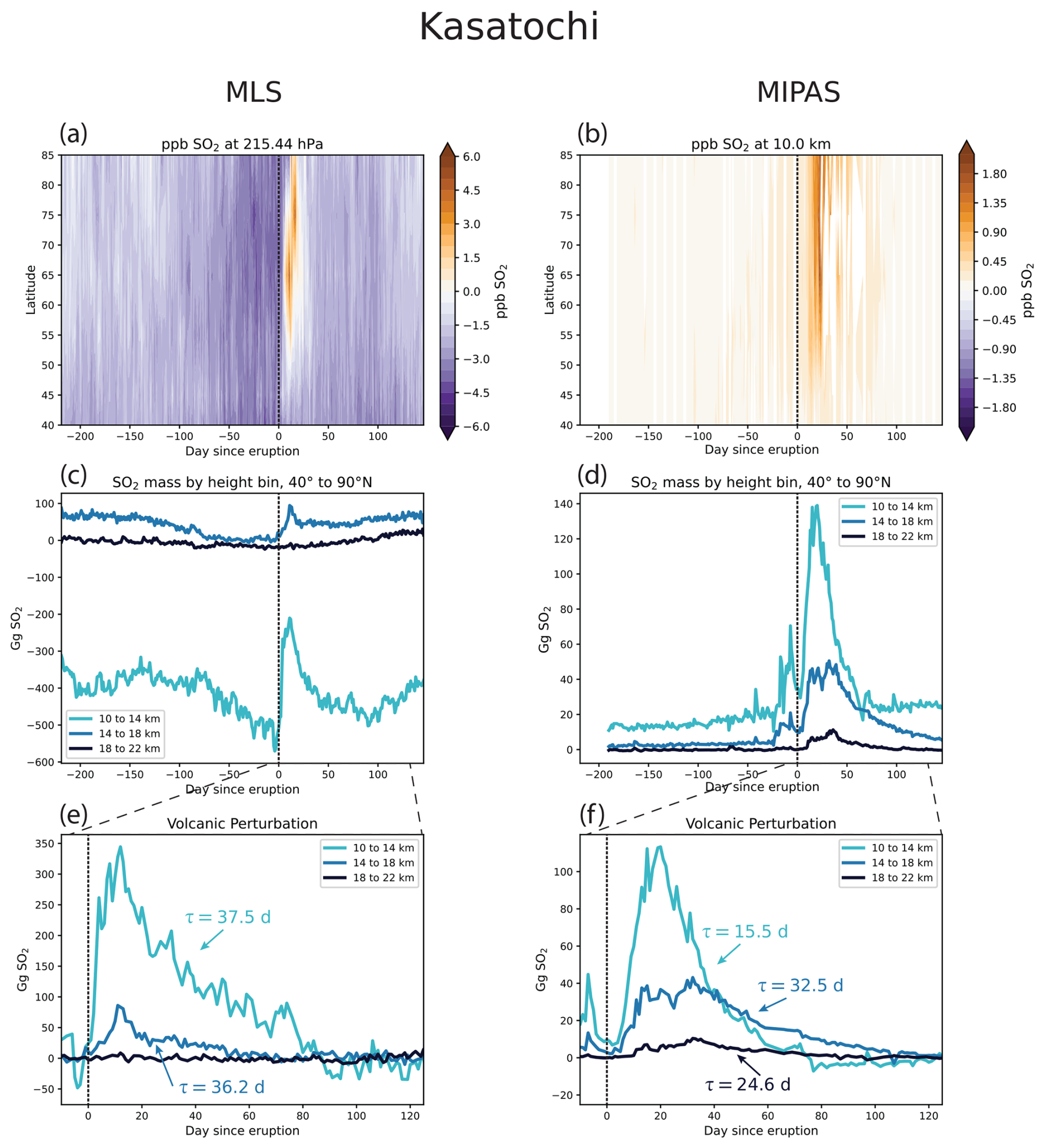
Figure 3 Comparison of MLS and MIPAS observations during 2008 and the Kasatochi eruption. MLS observations are shown in panels (a), (c), and (e); and MIPAS observations are shown in panels (b), (d) and (f). In all panels, day 0 corresponds to the start of the Kasatochi eruption (7 August 2008; Carn, 2025), as denoted by the vertical dashed line. Panels (a)–(b) show the volume mixing ratio in ppb as a function of latitude and time for the (a) MLS and (b) MIPAS at comparable altitudes on the native height coordinate of the respective observational product. Note the different color bar scale between the two panels. The mixing ratio values have been averaged for each day in 10° latitude bands but are otherwise unmodified from those reported in the respective datasets. Panels (c)–(d) show the mass of SO2 in Gg over the course of the year in the 10 to 14, 14 to 18, and 18 to 22 km height bins. Panels (e)–(f) show the perturbation of SO2 in each height bin resulting from the Kasatochi eruption and the associated decay timescales. There was no significant volcanic signal for the MLS data in the 18 to 22 height bin, and thus no values are reported. Note that in panels (c) and (e), the MLS data have been interpolated to the height coordinate of MIPAS.
Compared to MLS, the MIPAS data are easier to interpret. There is no significant seasonal cycle in the background, and the large injection of SO2 due to Kasatochi is clearly seen (Fig. 3d). Note that the spike in SO2 at lower altitudes prior to the Kasatochi eruption is likely due to the more minor eruption of Okmok in Alaska on 12 July 2008 (53.42° N, 168.13° W, 0.15 Tg SO2 emitted; Carn, 2025). The signal from this eruption is not clear in the MLS data.
However, the peak perturbation of SO2 after the Kasatochi eruption is roughly a factor of 3 greater in the MLS data than in the MIPAS data; this is because MIPAS does not fully sample the volcanic plume at its most dense. As noted by Höpfner et al. (2015), the difference between MIPAS and MLS in the initial part of the plume's dispersion and decay is thought to be the result of both interference from volcanic particles and saturation in the spectral lines measured by the MIPAS instrument in the presence of very high SO2 concentrations (such as those seen immediately after a large eruption). Thus, there are advantages and disadvantages to both satellite sensors in this application. MLS provides a better measurement of the peak input of SO2 relative to the MIPAS data. However, despite these shortcomings, the decay of the SO2 mass is clearly seen in MIPAS once the initial plume has dispersed enough for the signal to reach the instrument, i.e., when the SO2 radiance is no longer saturated. Furthermore, it is worth noting that the magnitude of the MLS values in version 5 of the data are roughly a factor of 4 smaller than those in version 2 reported by Pumphrey et al. (2015). The reason for this remains unclear, and no explanation or documentation for this difference was found in the literature.
We performed the same evaluation for the eruptions of Sarychev in 2009 (48.01° N, 153.20° W, 1.2 Tg SO2 emitted) and Nabro in 2011 (13.37° N, 41.70° E, 1.975 Tg SO2 emitted), the two other major eruptions covered by both MLS and MIPAS (Carn, 2025). The results for Sarychev and Nabro are shown in Figs. A1 and A2, respectively. In both cases, we see negative mixing ratios and masses in the lower two height bins in the MLS data. For Sarychev, the magnitude of the perturbation is comparable in MLS and MIPAS, with MIPAS showing around 100 Gg more mass in the 10–14 km height bin (Fig. A1e and f). Previously, Höpfner et al. (2015) indicated that MLS displayed more mass than MIPAS after Sarychev (their Fig. 13), and the change that we see here may be due to differences between version 2 and version 5 of the MLS data. Furthermore, in the case of the Nabro eruption, the MLS data in the 10 to 14 km height bin do not show any signal of the eruption. In the MIPAS data for Nabro, there is an upward trend in SO2 in the 10 to 14 km bin prior to the eruption. This could possibly be linked to the upward transport of SO2 in the Asian summer monsoon (Neely et al., 2014), as Nabro is a tropical eruption, and thus the latitude bands influenced by the eruption are also more likely to be influenced by the monsoon.
4.2 Background seasonal cycle in the MLS data
As shown in Fig. 3c, there is an apparent seasonal cycle in the mass of SO2 measured by MLS in both the 10 to 14 and 14 to 18 km height bins that is not realistic (Pumphrey et al., 2015; Höpfner et al., 2013). While Pumphrey et al. (2015) speculate that this is due to the leakage of information from O3 and HNO3, it is not obvious what the shape of the seasonal cycle should be, and we incorporate the resulting decay timescales corresponding to different possible seasonal cycles into an overall estimate of uncertainty in the decay timescale.
In order to sample possible shapes of the seasonal cycle, at each height bin we first take a 35 d running mean of the MLS time series with the non-volcanic background removed (see Sect. 2.4 for details on how we define the non-volcanic background). We then replace the values from day M to day N (where we vary M from −5 to 1 and N from 50 to 105 in the case of Kasatochi; we adjust the range of values for M and N for each eruption so that the seasonal cycles are reasonable) with a line between the SO2 mass on day M and the SO2 mass on day N. In other words, M and N define the section that we remove from the time series prior to determining the seasonal cycle, and varying these parameters results in different cycles. We then use a discrete fast Fourier transform to filter out the high-frequency variability, leaving us with the seasonal cycle. Once we determine this, we subtract the seasonal cycle from the time series.
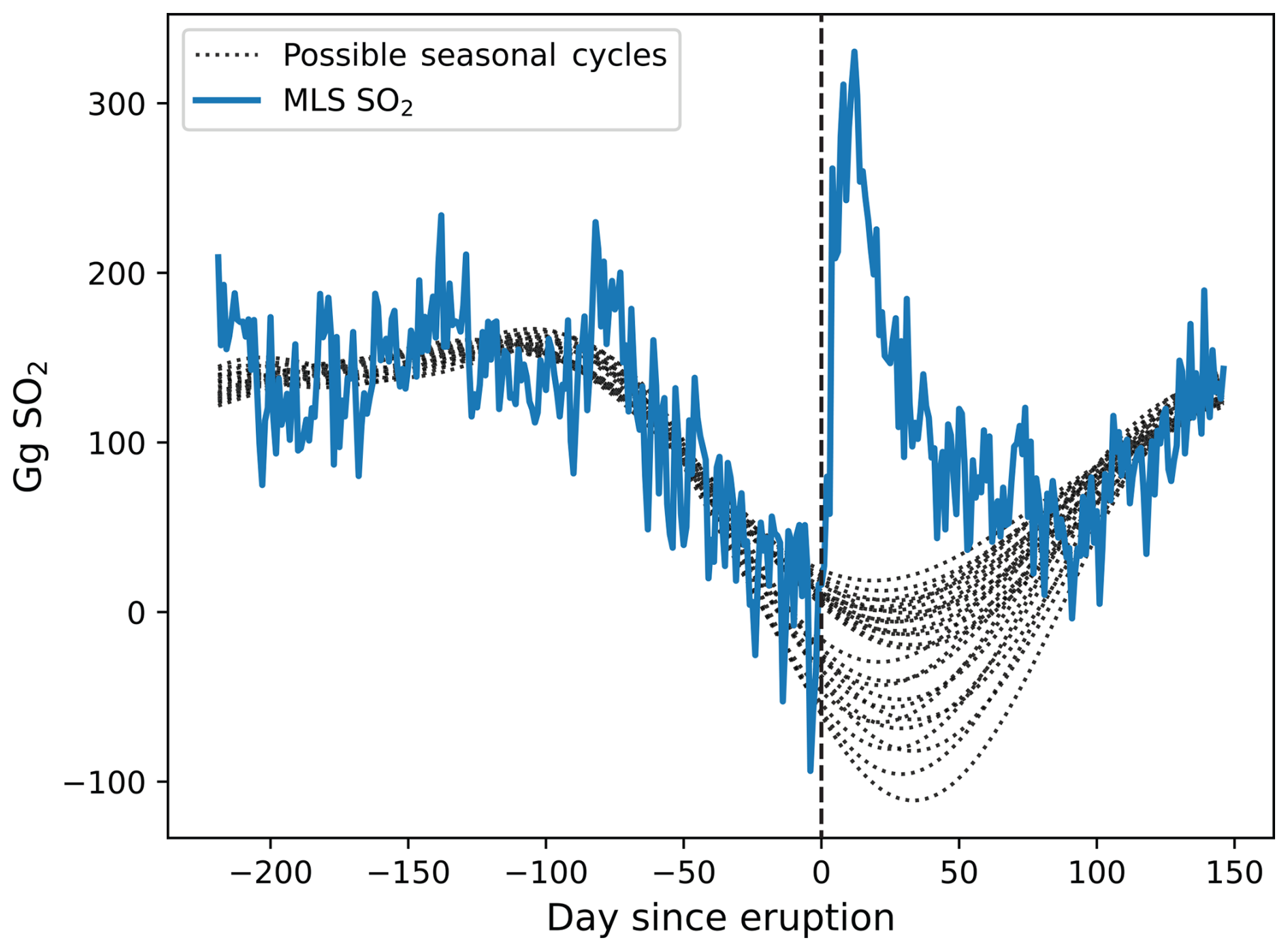
Figure 4 Possible background seasonal cycles in the MLS data. The blue curve shows MLS mass in the 10 to 14 km height bin following Kasatochi. Note that a constant has been subtracted from the time series shown in Fig. 3c so that the curve is roughly 0 immediately before the eruption. The dotted black lines show possible seasonal cycles that could have potentially occurred in the absence of the Kasatochi eruption. As in Fig. 3, day 0 corresponds to the eruption of Kasatochi and is indicated by the dashed vertical line.
Figure 4 demonstrates the possible seasonal cycles in the MLS data, derived using the method outlined above. The figure uses data from the Kasatochi eruption in the 10 to 14 km height bin, but the resulting spectrum of seasonal cycles is similar across eruptions and height bins. The presence of the seasonal cycle leads to a range of possibilities in the shape and decay of the volcanic perturbation, and this ultimately translates into greater uncertainty when deriving a decay timescale from the MLS data (see Sect. 4.3 and Table 1 for more details).
The approach outlined above samples possible seasonal cycles using the observed time series in a given year of an eruption. One could also potentially infer the interfering seasonal cycle from years without large volcanic eruptions; however, this presents its own challenges. There is a 100 to 200 Gg spread in SO2 mass on any given day of the year in non-volcanic conditions (Fig. S1 in the Supplement). Using the mean across years for the background seasonal cycle could result in an offset of ±50 to 100 Gg from the actual disturbing seasonal cycle. This difference is large enough to impart a significant bias in the estimated decay rate, thus limiting our ability to constrain the uncertainty. The seasonal cycle and inter-seasonal variability in MLS SO2 is interesting in its own right: it warrants further investigation and could potentially be calibrated based on the observed amounts of O3 and HNO3, but this is beyond the scope of the current paper.
4.3 Comparing SO2 decay timescales for different volcanoes
We compare decay timescales and their estimated uncertainties for MLS and MIPAS in Table 1 for the three largest eruptions during the time period covered by both products: Kasatochi in 2008, Sarychev in 2009, and Nabro in 2011. These eruptions all occurred in the local summer. However, Kasatochi and Sarychev are both high-latitude northern hemisphere eruptions, whereas Nabro is a tropical eruption. Differences in tropopause height, OH concentrations, and local dynamics between the tropics and higher latitudes make comparisons between Nabro and the high-latitude eruptions difficult. In particular, the tropopause in the tropics during the local summer is around 16 km, whereas for the high latitudes in the northern hemisphere it is closer to 11 km (Hoffmann and Spang, 2022). As a result, the majority of the three layers considered in this analysis are likely to be in the stratosphere for the Kasatochi and Sarychev eruptions. After the Nabro eruption, likely only the 18 to 22 km layer was initially fully in the stratosphere; however, the plume was quickly advected to higher latitudes – where the tropopause is lower – by the Asian monsoon anticyclone in just a few days (Clarisse et al., 2014). There are large vertical gradients in H2O and therefore OH at the tropopause (Milz et al., 2005; Jiang et al., 2015), and thus whether a layer falls above or below the tropopause will potentially significantly impact SO2 removal times. A more precise treatment of calculating SO2 decay based on whether a measurement falls above or below the tropopause is left for future work.
Despite this variability between different eruptions, the comparison between the observational products for a given eruption is illustrative of the uncertainty associated with each product. These values are summarized in Table 1. Values in bold indicate the median decay timescale from a collection of values calculated by varying the time window used for the linear fit of the exponential decay. Our uncertainty values (shown in parentheses) are the 5th and 95th percentiles, which gives a sense of the variability in the perturbation decay rate depending on how it is calculated. See Sect. 2.4 for more details on this calculation. Given the range of methods used to calculate the decay rate of volcanic SO2 in the literature (e.g., Höpfner et al., 2015, Table 3 and references therein), our intent with these uncertainty bounds is to demonstrate how a spread in the decay timescale can arise by changing the time period used for the calculation. Plume-induced changes in chemistry is one potential mechanism driving this behavior (McKeen et al., 1984). Vertical transport by the background circulation of the stratosphere is unlikely to have a significant impact on our results as it is quite slow – on the order of 10ths of mm s−1 or 100ths of km day−1 – compared to the timescale of SO2 decay (Butchart, 2014). Khaykin et al. (2022) did report an unusual radiative self-lofting of the Raikoke volcanic plume in 2019; the observed vertical ascent for this eruption was upwards of 2 mm s−1 (0.17 km d−1) and would be fast enough to impact our results. This phenomenon has not been noted for any of the volcanoes examined here, although it is a potential source of uncertainty and worth examining in future work.
In general, there is greater uncertainty in the MLS-derived decay timescales, in part because the ambiguity of the seasonal cycle present in the data is compounded by the variability that arises in changing the decay time window. The volcanic signals in the MIPAS data are clearer, and uncertainty in the decay timescale here stems from uncertainty in the exponential fit of the SO2 mass following the eruption alone. These results suggest that MIPAS, as an infrared sounder, can provide better estimates of the decay timescale throughout the depth of the atmosphere compared to MLS. However, we emphasize again that MIPAS does not capture the peak input as well as MLS.
Table 1Comparison of calculated decay timescales between this work and Höpfner et al. (2015). For the MIPAS, MLS, and WACCM rows, bold values are the median decay timescale, and the values in parentheses are the 5th and 95th percentiles. See Sects. 2.4 and 4.2 for more details on how these are calculated. MIPAS-derived values from Höpfner et al. (2015) are indicated by MIPAS H2015. Dashes indicate a lack of a clear signal for that product at that height bin. All timescales have units of days. The volcano names are in bold for readability.
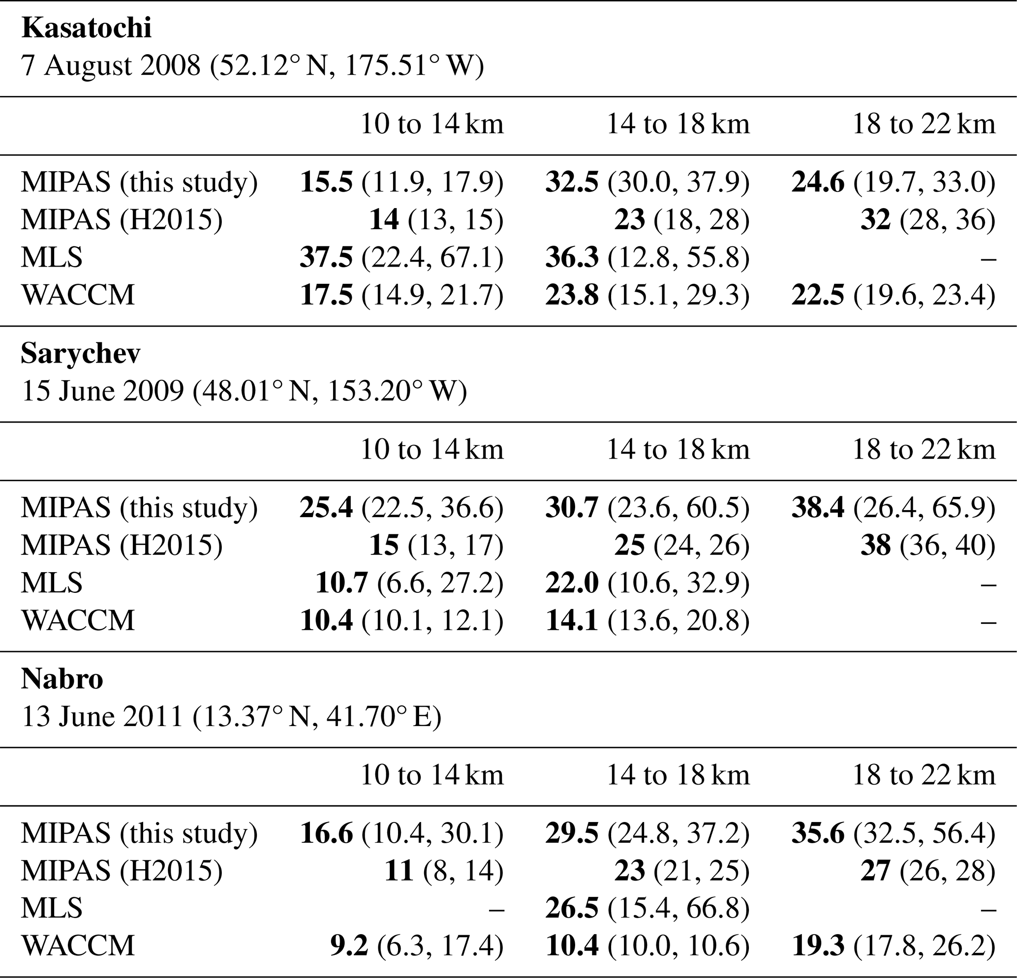
Table 1 also compares our calculated decay timescales with those calculated by Höpfner et al. (2015) using MIPAS retrievals. Note that Höpfner et al. (2015) refer to these values as “lifetimes”, calculating them by varying the window for the fit of a straight line to the natural logarithm of the SO2 mass. They use longer windows (around 30 d) than we use here. Their values show a clear increase of decay timescale with height, which is generally also seen in our results (with the exception of some of the values for Kasatochi). Additionally, the 5th to 95th percentile ranges reported here are large, and in nearly all cases the results reported in Höpfner et al. (2015) fall within the ranges given here.
We also compare the observations from the satellite products with output from the WACCM model (Gettelman et al., 2019) for these three eruptions (see Table 1 and Fig. 5). The WACCM model incorporates only gas-phase oxidation of SO2 and thus provides a useful baseline to use in comparing the real-world measurements.
The expected increase in decay timescale with height based on gas-phase oxidation alone is most obvious in the Nabro eruption for the WACCM data. In the satellite data, this is most clearly seen for MIPAS in the Sarychev and Nabro eruptions. The median WACCM decay timescales (in which OH is the only oxidative agent) tend to fall below the median decay timescales from the satellite observations. The one notable exception is the Sarychev eruption in the 10 to 14 km height bin, where the median decay timescales between MLS and WACCM are quite close, at around 11 d. However, it is challenging to make further conclusions from this alone due to the previously discussed issues in the MLS data. For Nabro, the median decay timescale from WACCM is outside the uncertainty range of the observations for all three height bins. There are a variety of potential causes for the discrepancy between the model and observations. One could be differences in water vapor and between the model and observations. However, comparisons between WACCM and MLS water vapor generally show strong agreement, and it is not clear that this should be the main culprit (Froidevaux et al., 2019). Model treatment of the interplay between particle scattering and photolysis inside the volcanic plume initially after the eruption could also play a role, but we do not explore this discrepancy further here.
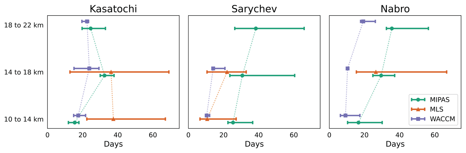
Figure 5 SO2 decay timescale in the 10 to 14, 14 to 18, and 18 to 22 km height bins for Kasatochi 2008, Sarychev 2009, and Nabro 2011. Markers indicate the median decay timescale, and error bars show the 5th and 95th percentiles. For a description of how the median and error bars are calculated, see Sects. 2.4 and 4.2. A missing data point for a given product and height bin indicates the lack of a sufficient signal for the calculation.
While the observed median decay timescale is generally on the order of 10 to 40 d, there is a wide range in values across the different products and height bins. The uncertainty in obtaining the decay timescale in the WACCM model is quite low, as it only arises due to uncertainty in the fitting of the decay. This decay is – as one would expect for model output – quite clear and easy to quantify; moreover, the tight bounds suggest that the removal of SO2 in the model is indeed exponential. However, uncertainties in the process understanding of OH chemistry in the model are likely to be a larger source of error; this likely also limits the interpretations of any discrepancies when comparing the observed data with model output. While MIPAS displays smaller uncertainties than MLS (Table 1), on the whole the observations have a much wider range of decay timescales. For example, the observational decay timescales in the 10 to 14 km height bin for Sarychev span from roughly 36 to under 7 d. For Kasatochi, the observational decay timescales in the 10 to 14 km height bin range from over 67 to under 12 d. It is also worth noting that previous estimates of decay timescales (derived using a variety of satellite products) for these eruptions do fall within the (rather large) uncertainty ranges shown here (see Höpfner et al., 2015, Table 3 and references therein).
We compare the results from MLS, MIPAS, and WACCM with SO2 retrievals from the Ozone Monitoring Instrument (OMI). OMI is a popular choice in recent work examining the decay of SO2 following eruptions (e.g., Carn et al., 2022; Zhu et al., 2020; Krotkov et al., 2010), and we include an analysis of it here for a comparison of how limb sounders and nadir sounders capture the removal of volcanic SO2. Note that OMI is just one of several nadir-sounding instruments that measure SO2, and a detailed comparison with other instruments (such as AIRS) is left to future work.
Unlike MLS and MIPAS, OMI is a nadir-viewing instrument that measures backscattered ultraviolet and visible radiation (Li et al., 2017). OMI reports the vertical column density of SO2 and lacks the detailed vertical resolution for SO2 provided by MLS and MIPAS. However, OMI is able to provide estimates of SO2 within different vertical layers of the atmosphere by assuming a vertical SO2 profile and iteratively adjusting it to fit the observed backscattered radiation. Here we use the stratospheric dataset from OMI, which is intended for studying explosive volcanic eruptions. For more details, see Sect. 2.1.3 and Li et al. (2017).
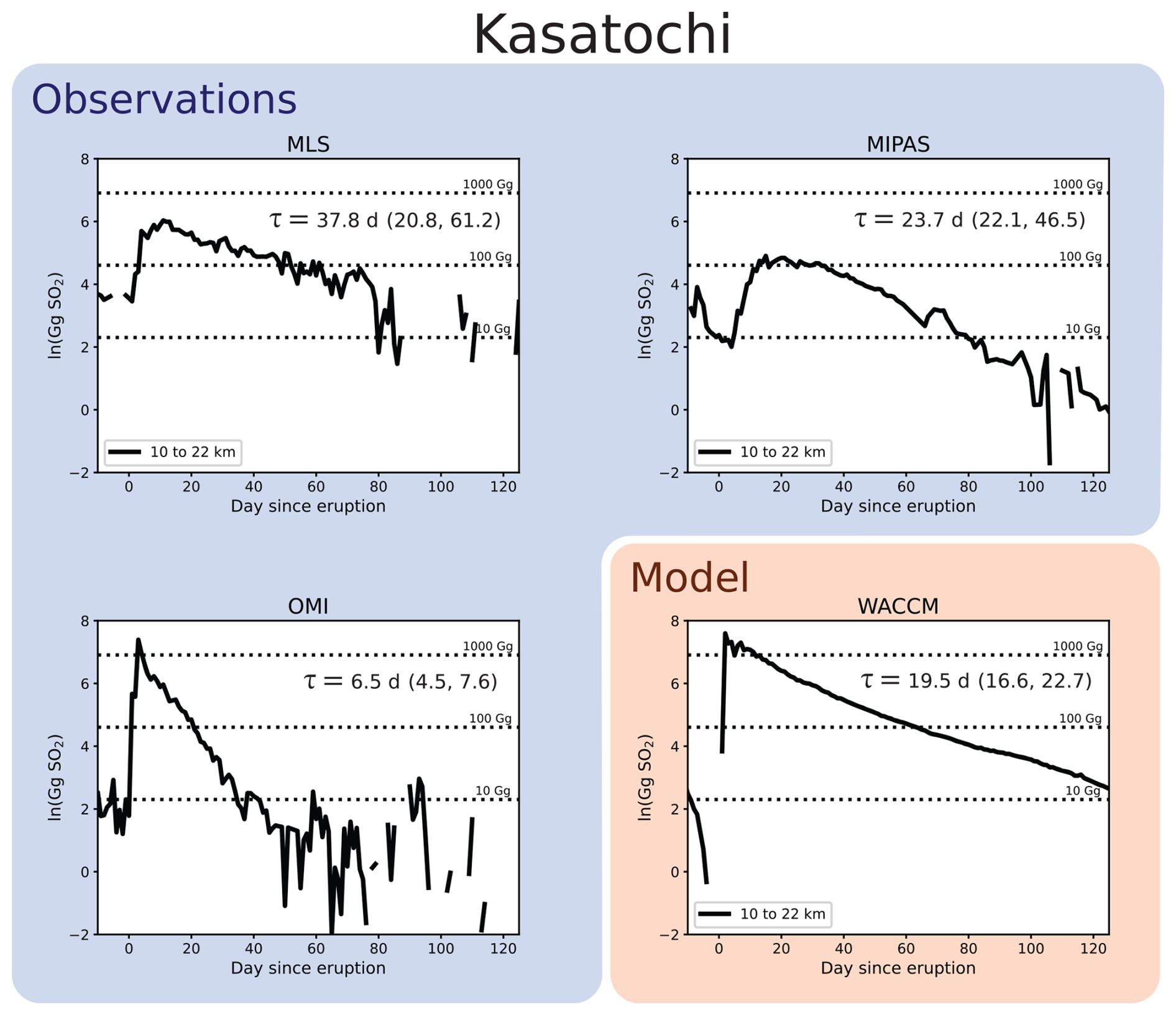
Figure 6Comparison of stratospheric decay timescales for the 2008 Kasatochi eruption. Satellite products are highlighted in blue and the WACCM model in orange. For comparison with the total column stratospheric values from OMI, SO2 masses for MLS, MIPAS, and WACCM are calculated by vertically integrating from 10 to 22 km. For each product, the median and 5th and 95th percentile (in parentheses) decay timescales are reported. Percentile ranges are derived using the method outlined in Sect. 2.4.
Since OMI provides only a total column perspective of the stratosphere, we compare the decay of the volcanic perturbation in OMI with that between 10 and 22 km in the MLS, MIPAS, and WACCM products. Figure 6 shows this comparison for the Kasatochi eruption. The OMI-derived decay timescale of 7.3 d is substantially faster than that in either of the other two satellite products or the WACCM model. Indeed, the 5th and 95th percentile range (6.0 to 8.8 d) for OMI does not overlap at all with this percentile range in any of the other products. Other published estimates of the OMI-derived decay timescale after Kasatochi are also similarly fast (Krotkov et al., 2010 report a time of 8 to 9 d).
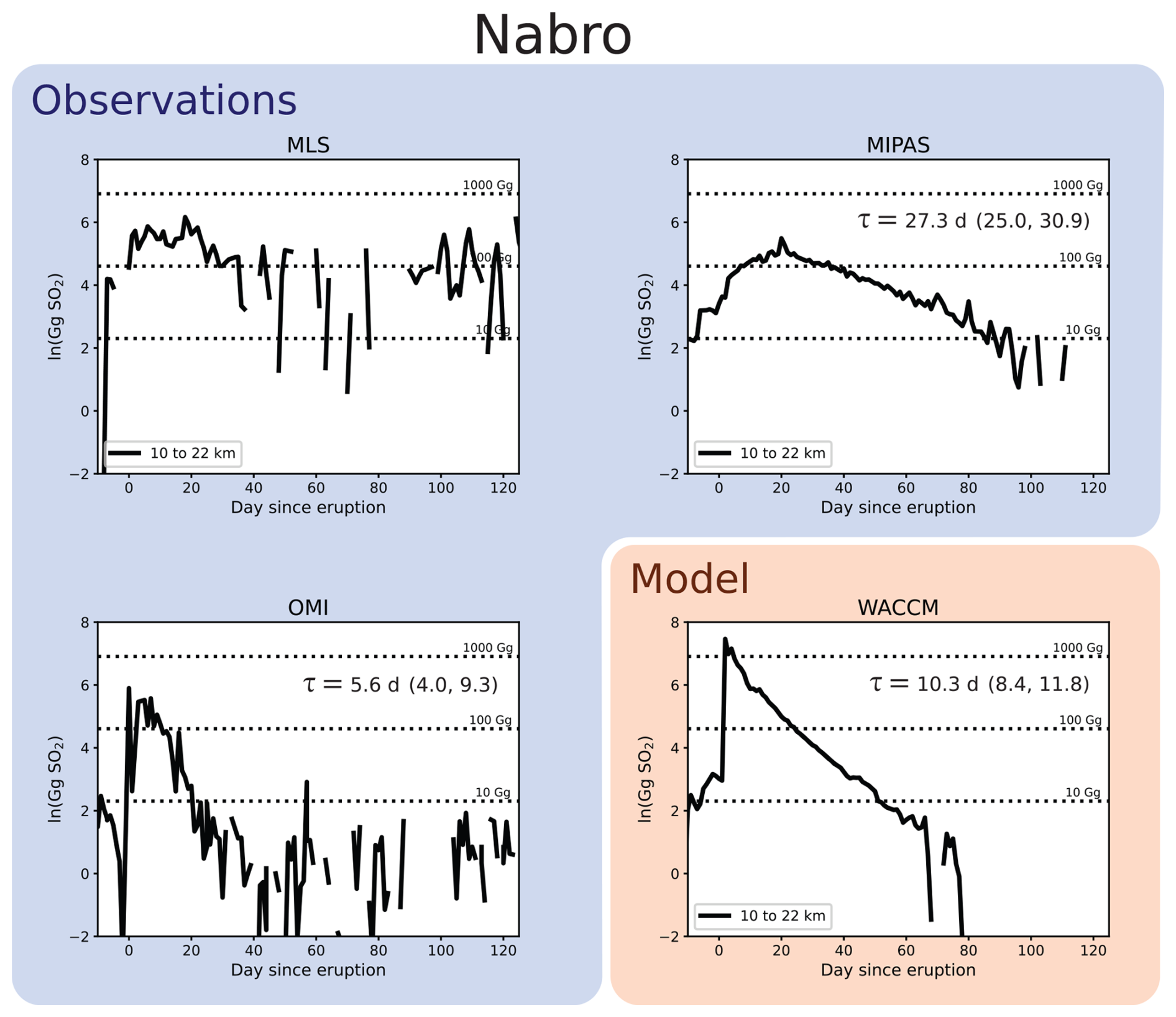
This difference in the OMI decay timescale also arises for the Sarychev and Nabro eruptions (Figs. B1 and B2, respectively). For both eruptions, the OMI value is much faster than either of the other three products, and there is nearly no overlap between the uncertainty ranges of OMI and the other products. There are a couple of possible explanations for this. While the OMI data used here are designed to give an estimate of SO2 mass in the stratosphere (Sect. 2.1.3), there is the potential for tropospheric SO2 to influence this measurement. Tropospheric SO2 will generally get removed much quicker than that in the stratosphere and could be skewing the decay rates reported here. Additionally, there is a known bias in the OMI data due to the limited sensitivity of nadir instruments as the plume disperses (see Sect. 2.1). Both of these should be considered more carefully when analyzing OMI SO2 following an eruption.
As an aside, we also comment on the differences between the model and MIPAS for the three eruptions. In the Kasatochi eruption, the discrepancy in the 10 to 22 km decay timescale between the model and MIPAS is much less than the other two eruptions (see Figs. 6, B1, and B2). One plausible explanation for this is that the model puts a significant fraction of the SO2 from Kasatochi into the 14 to 18 km height bin, whereas for Sarychev and Nabro, there is relatively more mass in the 10 to 14 km height bin (Fig. S2). As OH decreases with height in the model, this would lead to slower (and thus closer to MIPAS) decay times for the Kasatochi SO2 when the larger vertical column is considered.
In addition to understanding the chemical fate of volcanically emitted SO2, quantifying its total stratospheric burden is key to understanding the potential climate and chemical impacts of volcanic eruptions (Schmidt et al., 2018; Solomon et al., 1998). Carn et al. (2016) provide a review of total SO2 mass loading from volcanic eruptions occurring from 1978 through 2014. These values are largely derived from nadir instruments (i.e., TOMS, OMI, IASI) and are often used as the standard reference for volcanic SO2 mass loading. Carn (2025) provides an updated dataset of volcanic SO2 injections into the stratosphere through 2024, which we use as a benchmark for our estimates.
The eruptions analyzed in this work (Kasatochi, 2008; Sarychev, 2009; and Nabro 2011) feature a high plume height and high VEI, which allowed the eruptions to inject upwards of 1 Tg into the stratosphere, as reported by nadir sounders (Carn, 2025; Carboni et al., 2016). Table 2 compares the SO2 stratospheric mass loading for Kasatochi, Sarychev, and Nabro, derived in this study from satellite observations with previously published values.
We estimate the total stratospheric SO2 burden after an eruption via two different methods. The first, referred to as “total increase” in Table 2, uses the time series shown in Figs. 6, B1, and B2. For MLS and MIPAS, these are the time series of SO2 in the 10 to 22 km height bin. For each eruption's time series, we take the difference between each successive data point (i.e., np.diff) and sum the positive values of the resulting array during the eruption period for each eruption. The eruption period is based on volcanic activity reports provided by Venzke (2024). In the event that the maximum SO2 mass occurs outside of the eruption period (e.g., Kasatochi erupted for only 2 d, but peak SO2 in the MIPAS dataset occurs after this), we sum the positive values of the differences until the day of maximum SO2.
As discussed in more detail below, this method proves inadequate for accurate mass burden estimations. This is particularly true for MIPAS, as the spectral bands measured by MIPAS saturate at high SO2 concentrations. The inclusion of this method in this paper provides a contrast compared to previously published total burden estimates derived from SO2 decay timescale estimates (e.g., Höpfner et al., 2015; Pumphrey et al., 2015, for MIPAS and MLS, respectively). This previous work estimates the mass of SO2 immediately after the eruption by fitting an exponential curve to the decay of SO2. The mass at t=0 is then taken to be the total SO2 emitted by the volcano. We use this same method (indicated as “decay fit” in Table 2), where the window used for the decay timescale calculation is varied, as discussed previously. We report both a median mass loading and the 5th and 95th percentiles to give a sense of the spread in the estimate.
Carn (2025)Carn (2025)Carn (2025)Table 2Estimated total SO2 mass emitted into the stratosphere. For values calculated in this study, the utilized method is listed. Values from Höpfner et al. (2015) are indicated by H2015, and those from Pumphrey et al. (2015) are indicated by P2015. There was not a sufficient signal to calculate the extrapolated SO2 for Nabro using MLS. For values calculated in this paper, parentheses indicate the 5th and 95th percentiles. The volcano names are in bold for readability.
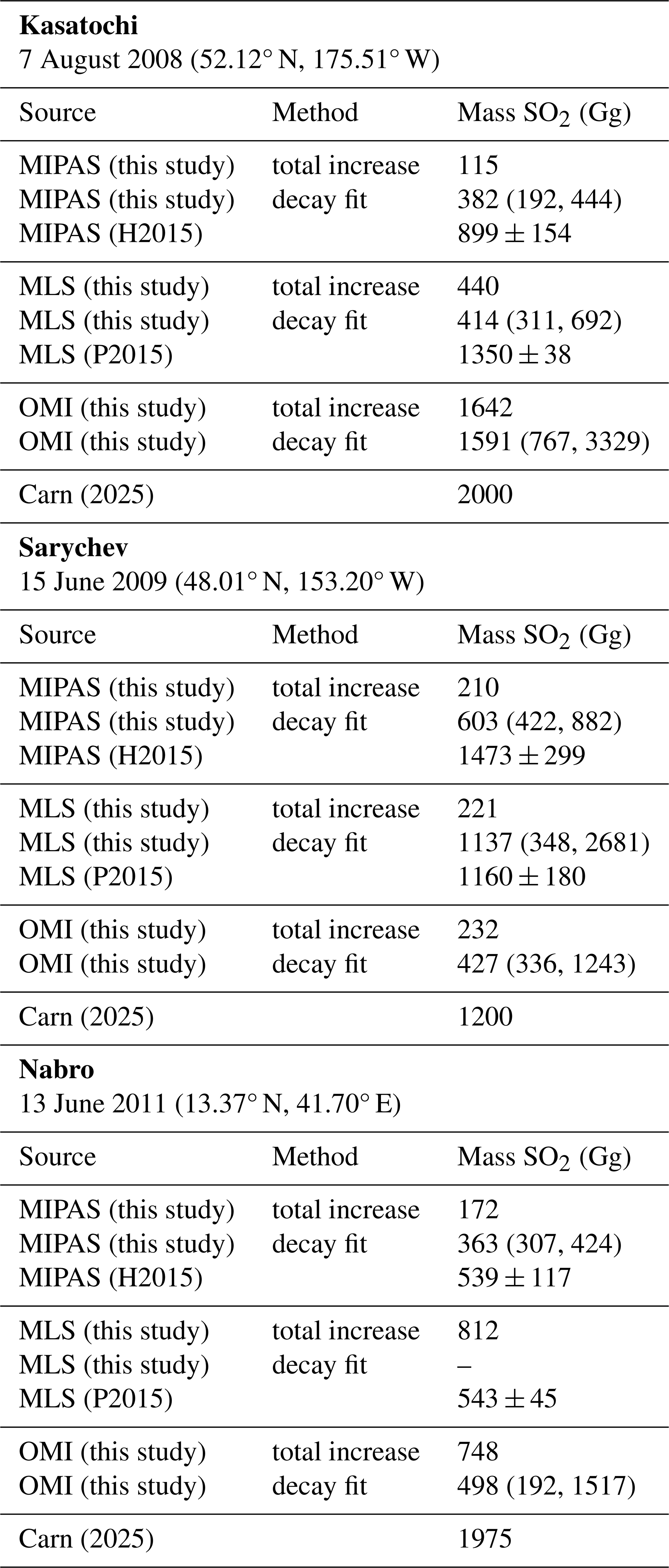
The masses calculated using the total increase method are generally much lower than those given by Carn (2025), and with the exception of Sarychev, there is limited agreement between the observational products. While this approach avoids the uncertainty associated with using decay timescales to determine total mass burden, we do not find it adequate for an accurate determination of the total mass. This is particularly true of MIPAS due to its previously mentioned shortfall: it underestimates the total amount of SO2 present at the start of the eruption when the plume is dense. Despite these shortcomings, this method does clearly illustrate how the different satellites capture the peak SO2.
The total increase values reported here, with the exception of OMI during the Kasatochi eruption, are also not high enough to account for the observed aerosol loading and radiative forcing following the eruptions (Schmidt et al., 2018). However, despite the noise and interference issues, for Kasatochi and Nabro, MLS does get closer to the expected mass burden than MIPAS (although MLS still underestimates it significantly).
Previous estimates of total SO2 using the decay fit method have generally led to good results for MIPAS and MLS when compared to other estimates (Höpfner et al., 2015; Pumphrey et al., 2015); however, the final value will be sensitive to how the exponential fit is calculated. As discussed previously, the details of this calculation can result in wide variability in the decay timescale (e.g., Fig. 6), and this directly translates to uncertainty in the mass loading. The SO2 burdens calculated using the decay fit method in Table 2 highlight this. Moreover, a physical reason for this uncertainty could be the large range of decay timescales observed in the initial dense volcanic plume (McKeen et al., 1984); a better understanding of variations in the SO2 oxidation rate within the lifetime of a given plume could help to reduce this uncertainty.
We also note that the MIPAS and MLS SO2 masses in some eruptions are significantly lower compared to the Carn (2025) values. Whether this reflects fractional stratospheric inputs or biases due to limitations of sampling by limb-sounding instruments would be a subject for future research. Additionally, our masses from MIPAS are lower than those reported in Höpfner et al. (2015). This is perhaps due to differences in the way the calculations are done. In Höpfner et al. (2015), masses are calculated (via an exponential fit) in 4 km height layers and then summed to get the total stratospheric burden. Here we calculate the burden by calculating the masses from 10 to 22 km and then applying the fit. Indeed, if we apply our method to the results shown in Fig. 14 in Höpfner et al. (2015) (their plot of total stratospheric SO2 burden after Sarychev), the resulting mass is comparable to what we report here.
Finally, we highlight the fact that the uncertainty ranges for OMI are quite large, and this is due to the rapid decay timescales reported for OMI. Even though the spread among these timescales for a given eruption is low, the nature of the exponential fit means that the initial burden will be more sensitive to changes in the decay timescale when the timescale is faster.
The main focus of the paper is on the decay times of the stratospheric SO2 inputs from the indicated eruptions, and Table 2 explores the implications of such information for estimating the total stratospheric mass burden. Future work in this direction should consider the uncertainty in the decay timescale when fitting the curve with an exponential. Furthermore, our results indicate that simply summing the positive SO2 perturbations from a volcano is not sufficient for getting an accurate mass burden in the datasets analyzed here.
Quantifying the total input and decay timescale of SO2 is a key step in understanding the chemical fate of volcanically emitted SO2 in the stratosphere. In this work, we utilize a combination of satellite products and a coupled chemistry-climate model to analyze the decay of the SO2 perturbation from the three largest eruptions between 2004 and 2012: Kasatochi in 2008, Sarychev in 2009, and Nabro in 2011. This is the time period covered by all three of the satellite products used in this work. Smaller eruptions during this time period (e.g., Cordon Caulle, Grimsvötn, Redoubt) were not included due to the difficulty of detecting a clear decay of SO2 in the MLS dataset.
We compared the results between the Michelson Interferometer for Passive Atmospheric Sounding (MIPAS) and the Microwave Limb Sounder (MLS). Both limb-sounding instruments, the SO2 retrievals from these products allow for a vertically resolved analysis of the decay timescale. We report decay timescales in three different height bins (the same ones used by Höpfner et al., 2015): 10 to 14, 14 to 18, and 18 to 22 km. In general, we find that uncertainty in the decay timescale is much larger in the MLS dataset than in MIPAS. This is primarily a consequence of apparent interferences in the background seasonal cycle in the MLS data. While this seasonal cycle has been noted in previous work (Pumphrey et al., 2015) and is likely due to HNO3 and O3, it is not obvious what the form of the seasonal cycle should be, and this makes it inherently challenging to accurately determine the shape and magnitude of the volcanic perturbation. Furthermore, the MLS data are much noisier than the MIPAS data and feature large negative values in the SO2 mixing ratio. We suggest that the noise and negative bias is a consequence of pressure broadening; microwave emissions are more subject to pressure broadening, which obscures the signal received by the MLS instrument. This is further supported by the fact that the noise and negative bias are far less significant in the 18 to 22 km height bin (Fig. 3); the impacts of pressure broadening decrease with altitude (Pierrehumbert, 2010). Comparisons of the vertically resolved decay timescales between satellite observations and a global climate chemistry model (WACCM; Gettelman et al., 2019) indicate that the model generally predicts a faster decay timescale than the observations show, particularly at higher altitudes (Fig. 5). The 5th to 95th percentile range of decay timescales in the model also tends to be narrower than the observations. The reasons for these discrepancies require future investigation.
We also compare the decay timescales of SO2 within the whole stratospheric column. Here we include an additional observational dataset from the Ozone Monitoring Instrument (OMI), which is a common choice for analyzing volcanic SO2 decay (e.g., Carn et al., 2022; Zhu et al., 2020; Krotkov et al., 2010). We find that the timescale in the OMI dataset is consistently the fastest across the three eruptions analyzed. The uncertainty range of the OMI data only minimally overlaps with the uncertainty ranges of any of the other three products for the Nabro eruption, suggesting that OMI might overestimate the rate of stratospheric SO2 decay following an eruption. This is a bias, perhaps due to interference from tropospheric SO2 and nadir instruments' limited sensitivity to dispersed plumes. This should be considered when analyzing volcanic SO2 with OMI and other nadir-sounding instruments.
The range of decay timescales also limits the ability to accurately determine the initial mass loading following an eruption when using a constant decay timescale to extrapolate the SO2 data back to the start of day of the eruption. Both Pumphrey et al. (2015) and Höpfner et al. (2015) utilize exponential fits to evaluate the initial SO2 burden in MLS and MIPAS, respectively. However, the significant variations in the decay timescale reported in this work translate to similar uncertainty in the total mass of SO2 emitted by the volcano. This is a key quantity for understanding the climate and chemical impacts of volcanic eruptions, and this work suggests that constraining it using an exponential fit potentially comes with significant uncertainties.
The high variability in decay timescales across observational products and the lack of consensus with the WACCM model makes it difficult to assess whether differences in the decay timescale from one eruption to the next are due to different oxidation processes or just the result of dynamics and the inherent difficulty of constraining and observing volcanic plumes. Zhu et al. (2020) argued that the relatively short decay timescale of approximately 7 d was indicative of heterogeneous oxidation on ash being an important process after the Kelut eruption in 2014. Kelut, like Nabro, was a tropical eruption but was known to inject large amounts of ash into the atmosphere that persisted for longer than usual (Vernier et al., 2016). The observations of Nabro in the 14 to 18 km height bin suggest longer SO2 decay timescales ranging from about 10 to over 60 d, indicating that the ash effect, if indeed significant, may well be specific to certain eruptions. Moreover, Zhu et al. (2020) use OMI data in their analysis, and as shown here, OMI results in fast decay timescales compared to MLS or MIPAS. Note that we do not present an analysis of Kelut in this paper, as the MLS data for that eruption lacked a strong signal (not shown), and the MIPAS data ended in 2012, prior to the eruption of Kelut.
The eruption of Hunga in 2022 has also been noted for its remarkably fast SO2 e-folding time (Asher et al., 2023; Zhu et al., 2022). A submarine volcano, Hunga injected an estimated 150 Tg water vapor (H2O) and 0.41 ± 0.01 Tg SO2 into the stratosphere, and the rapid decay of SO2 has been attributed to a significant increase in OH following the H2O injection (Asher et al., 2023). The plumes from the eruptions also reached over 30 km above the surface (Asher et al., 2023). Given the unusual nature of the eruption, we do not include a quantitative analysis of it here. Rather, we mention it as a further example of the possible variability in the conditions influencing volcanic SO2 oxidation.
Our work suggests that the current SO2 data reported by the available observational products are subject to significant uncertainty when examining the stratospheric decay of volcanic SO2. The varying strengths and shortcomings of the different observational products should be accounted for when using them to determine chemical mechanisms and SO2 mass loading. Furthermore, the forthcoming loss of MLS (the only limb-sounding SO2 instrument in operation with continuous coverage over global latitudes and longitudes) will leave a significant gap in our ability to monitor the stratosphere.
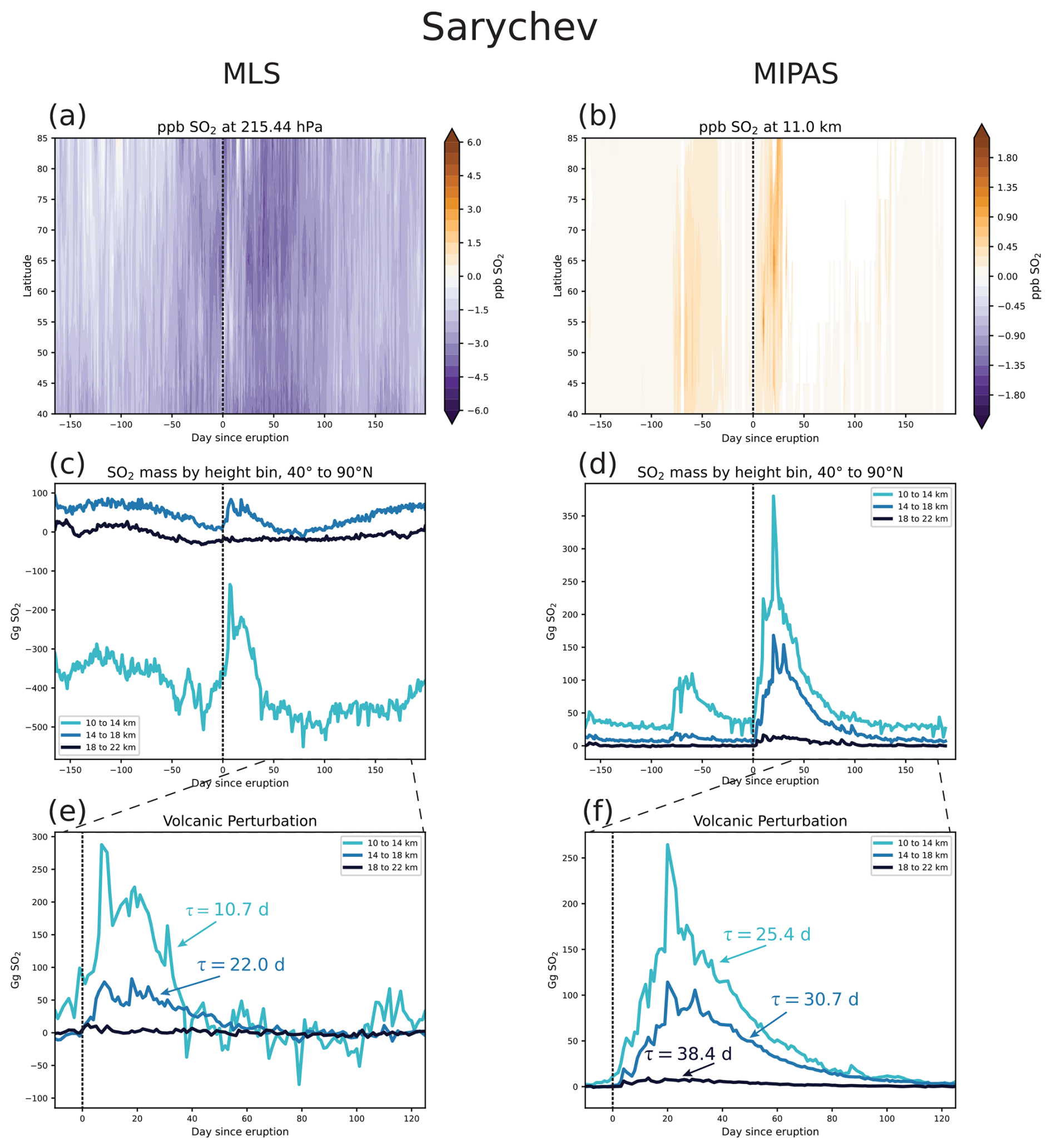
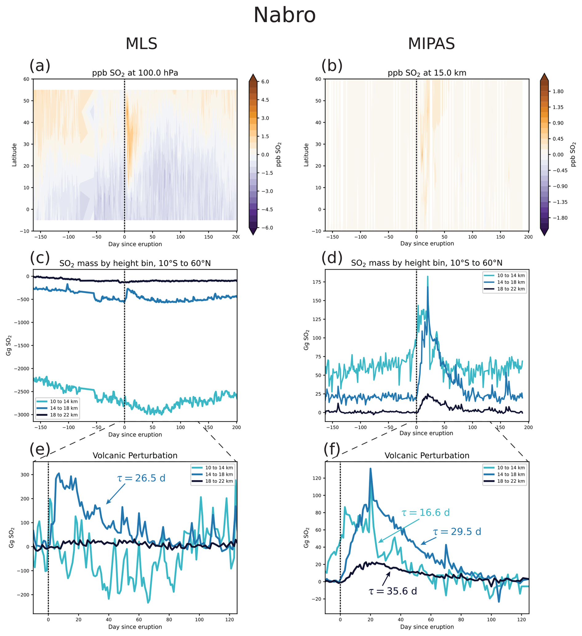
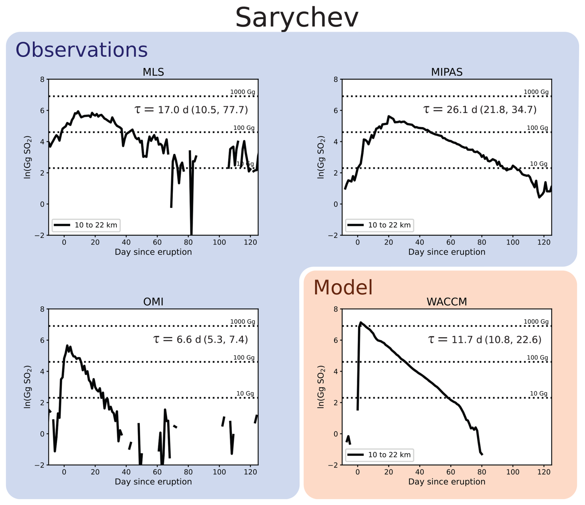
Figure B1 Comparison of stratospheric decay timescales for the 2009 Sarychev eruption, using the same format as Fig. 6.
All satellite data used in this study are publicly available:
-
MIPAS (with registration) – https://www.imk-asf.kit.edu/english/308.php (KIT (Karlsruhe Institute of Technology), 2024);
-
MLS – https://doi.org/10.5067/Aura/MLS/DATA2519 (Read and Livesey, 2021);
-
OMI – https://doi.org/10.5067/Aura/OMI/DATA2022 (Li et al., 2020).
Scripts for the main computations in the paper can be found at https://doi.org/10.5281/zenodo.17180491 (Nicknish, 2025). CESM2-WACCM6 data can be provided upon request.
The supplement related to this article is available online at https://doi.org/10.5194/acp-25-11535-2025-supplement.
PAN and SS developed the study, and PAN conducted the analysis with input from KS and SS. All authors contributed to the writing and revision of the paper.
The contact author has declared that none of the authors has any competing interests.
Publisher’s note: Copernicus Publications remains neutral with regard to jurisdictional claims made in the text, published maps, institutional affiliations, or any other geographical representation in this paper. While Copernicus Publications makes every effort to include appropriate place names, the final responsibility lies with the authors.
The authors would like to thank Hugh Pumphrey for helpful conversations and insights during the research process. The computations presented here were conducted using the “Svante” cluster, a facility located at MIT's Massachusetts Green High Performance Computing Center and supported by the Center for Sustainability Science and Strategy (https://cs3.mit.edu, last access: 23 September 2025). We would also like to acknowledge computing support from the Casper system (https://ncar.pub/casper, last access: 23 September 2025) provided by the NSF National Center for Atmospheric Research (NCAR), sponsored by the National Science Foundation. Additionally, the authors would like to thank the two anonymous reviewers and the handling editor for their helpful comments and feedback during the review process.
Paul A. Nicknish has been supported by the Presidential Graduate Fellowship at MIT and the National Science Foundation Graduate Research Fellowship under grant no. 2141064. Simon A. Carn has been supported by the NASA MEaSUREs program (grant no. 80NSSC24K0922). Susan Solomon has been supported by the NSF (grant no. 2316980).
This paper was edited by Matthew Toohey and reviewed by two anonymous referees.
Asher, E., Todt, M., Rosenlof, K., Thornberry, T., Gao, R.-S., Taha, G., Walter, P., Alvarez, S., Flynn, J., Davis, S. M., Evan, S., Brioude, J., Metzger, J.-M., Hurst, D. F., Hall, E., and Xiong, K.: Unexpectedly rapid aerosol formation in the Hunga Tonga plume, P. Natl. Acad. Sci. USA, 120, e2219547120, https://doi.org/10.1073/pnas.2219547120, 2023. a, b, c
Brasseur, G. and Solomon, S.: Aeronomy of the middle atmosphere: chemistry and physics of the stratosphere and mesosphere, no. 32 in Atmospheric and oceanographic sciences library, Springer, Dordrecht, Great Britain, 3rd rev. and enlarged ed edn., ISBN 978-1-4020-3284-4 978-1-4020-3824-2, 2005. a, b
Butchart, N.: The Brewer-Dobson circulation, Rev. Geophys., 52, 157–184, https://doi.org/10.1002/2013RG000448, 2014. a
Carboni, E., Grainger, R. G., Mather, T. A., Pyle, D. M., Thomas, G. E., Siddans, R., Smith, A. J. A., Dudhia, A., Koukouli, M. E., and Balis, D.: The vertical distribution of volcanic SO2 plumes measured by IASI, Atmos. Chem. Phys., 16, 4343–4367, https://doi.org/10.5194/acp-16-4343-2016, 2016. a
Carey, S. and Bursik, M.: Volcanic Plumes, in: Encyclopedia of Volcanoes, Elsevier, 571–585, https://doi.org/10.1016/B978-0-12-385938-9.00032-8, 2015. a
Carn, S.: Multi-Satellite Volcanic Sulfur Dioxide L4 Long-Term Global Database V4, Goddard Earth Science Data and Information Services Center (GES DISC) [data set], Greenbelt, MD, USA, https://doi.org/10.5067/MEASURES/SO2/DATA405, 2025. a, b, c, d, e, f, g, h, i, j, k, l
Carn, S., Clarisse, L., and Prata, A.: Multi-decadal satellite measurements of global volcanic degassing, J. Volcanol. Geoth. Res., 311, 99–134, https://doi.org/10.1016/j.jvolgeores.2016.01.002, 2016. a, b, c, d, e
Carn, S. A., Krotkov, N. A., Fisher, B. L., and Li, C.: Out of the blue: Volcanic SO2 emissions during the 2021–2022 eruptions of Hunga Tonga-Hunga Ha'apai (Tonga), Front. Earth Sci., 10, 976962, https://doi.org/10.3389/feart.2022.976962, 2022. a, b, c
Clarisse, L., Coheur, P.-F., Theys, N., Hurtmans, D., and Clerbaux, C.: The 2011 Nabro eruption, a SO2 plume height analysis using IASI measurements, Atmos. Chem. Phys., 14, 3095–3111, https://doi.org/10.5194/acp-14-3095-2014, 2014. a, b
Fischer, H., Birk, M., Blom, C., Carli, B., Carlotti, M., von Clarmann, T., Delbouille, L., Dudhia, A., Ehhalt, D., Endemann, M., Flaud, J. M., Gessner, R., Kleinert, A., Koopman, R., Langen, J., López-Puertas, M., Mosner, P., Nett, H., Oelhaf, H., Perron, G., Remedios, J., Ridolfi, M., Stiller, G., and Zander, R.: MIPAS: an instrument for atmospheric and climate research, Atmos. Chem. Phys., 8, 2151–2188, https://doi.org/10.5194/acp-8-2151-2008, 2008. a
Froidevaux, L., Kinnison, D. E., Wang, R., Anderson, J., and Fuller, R. A.: Evaluation of CESM1 (WACCM) free-running and specified dynamics atmospheric composition simulations using global multispecies satellite data records, Atmos. Chem. Phys., 19, 4783–4821, https://doi.org/10.5194/acp-19-4783-2019, 2019. a
Gettelman, A., Mills, M. J., Kinnison, D. E., Garcia, R. R., Smith, A. K., Marsh, D. R., Tilmes, S., Vitt, F., Bardeen, C. G., McInerny, J., Liu, H., Solomon, S. C., Polvani, L. M., Emmons, L. K., Lamarque, J., Richter, J. H., Glanville, A. S., Bacmeister, J. T., Phillips, A. S., Neale, R. B., Simpson, I. R., DuVivier, A. K., Hodzic, A., and Randel, W. J.: The Whole Atmosphere Community Climate Model Version 6 (WACCM6), J. Geophys. Res.-Atmos., 124, 12380–12403, https://doi.org/10.1029/2019JD030943, 2019. a, b, c
Glaze, L. S., Baloga, S. M., and Wilson, L.: Transport of atmospheric water vapor by volcanic eruption columns, J. Geophys. Res.-Atmos., 102, 6099–6108, https://doi.org/10.1029/96JD03125, 1997. a
Günther, A., Höpfner, M., Sinnhuber, B.-M., Griessbach, S., Deshler, T., von Clarmann, T., and Stiller, G.: MIPAS observations of volcanic sulfate aerosol and sulfur dioxide in the stratosphere, Atmos. Chem. Phys., 18, 1217–1239, https://doi.org/10.5194/acp-18-1217-2018, 2018. a, b, c, d
Hoffmann, L. and Spang, R.: An assessment of tropopause characteristics of the ERA5 and ERA-Interim meteorological reanalyses, Atmos. Chem. Phys., 22, 4019–4046, https://doi.org/10.5194/acp-22-4019-2022, 2022. a, b
Höpfner, M., Glatthor, N., Grabowski, U., Kellmann, S., Kiefer, M., Linden, A., Orphal, J., Stiller, G., von Clarmann, T., Funke, B., and Boone, C. D.: Sulfur dioxide (SO2) as observed by MIPAS/Envisat: temporal development and spatial distribution at 15–45 km altitude, Atmos. Chem. Phys., 13, 10405–10423, https://doi.org/10.5194/acp-13-10405-2013, 2013. a, b, c
Höpfner, M., Boone, C. D., Funke, B., Glatthor, N., Grabowski, U., Günther, A., Kellmann, S., Kiefer, M., Linden, A., Lossow, S., Pumphrey, H. C., Read, W. G., Roiger, A., Stiller, G., Schlager, H., von Clarmann, T., and Wissmüller, K.: Sulfur dioxide (SO2) from MIPAS in the upper troposphere and lower stratosphere 2002–2012, Atmos. Chem. Phys., 15, 7017–7037, https://doi.org/10.5194/acp-15-7017-2015, 2015. a, b, c, d, e, f, g, h, i, j, k, l, m, n, o, p, q, r, s, t, u, v, w, x, y, z, aa
Jiang, J. H., Su, H., Zhai, C., Wu, L., Minschwaner, K., Molod, A. M., and Tompkins, A. M.: An assessment of upper troposphere and lower stratosphere water vapor in MERRA, MERRA2, and ECMWF reanalyses using Aura MLS observations, J. Geophys. Res.-Atmos., 120, 11468–11485, https://doi.org/10.1002/2015JD023752, 2015. a
Karu, E., Li, M., Ernle, L., Brenninkmeijer, C. A. M., Lelieveld, J., and Williams, J.: Carbonyl Sulfide (OCS) in the Upper Troposphere/Lowermost Stratosphere (UT/LMS) Region: Estimates of Lifetimes and Fluxes, Geophys. Res. Lett., 50, e2023GL105826, https://doi.org/10.1029/2023GL105826, 2023. a
Khaykin, S. M., De Laat, A. T. J., Godin-Beekmann, S., Hauchecorne, A., and Ratynski, M.: Unexpected self-lofting and dynamical confinement of volcanic plumes: the Raikoke 2019 case, Sci. Rep., 12, 22409, https://doi.org/10.1038/s41598-022-27021-0, 2022. a
KIT (Karlsruhe Institute of Technology): Access to IMK/IAA generated MIPAS/Envisat data, KIT, https://www.imk-asf.kit.edu/english/308.php (last access: 20 May 2024), 2024. a
Kremser, S., Thomason, L. W., Von Hobe, M., Hermann, M., Deshler, T., Timmreck, C., Toohey, M., Stenke, A., Schwarz, J. P., Weigel, R., Fueglistaler, S., Prata, F. J., Vernier, J.-P., Schlager, H., Barnes, J. E., Antuña-Marrero, J.-C., Fairlie, D., Palm, M., Mahieu, E., Notholt, J., Rex, M., Bingen, C., Vanhellemont, F., Bourassa, A., Plane, J. M. C., Klocke, D., Carn, S. A., Clarisse, L., Trickl, T., Neely, R., James, A. D., Rieger, L., Wilson, J. C., and Meland, B.: Stratospheric aerosol-Observations, processes, and impact on climate: Stratospheric Aerosol, Rev. Geophys., 54, 278–335, https://doi.org/10.1002/2015RG000511, 2016. a, b, c
Krotkov, N. A., Schoeberl, M. R., Morris, G. A., Carn, S., and Yang, K.: Dispersion and lifetime of the SO2 cloud from the August 2008 Kasatochi eruption, J. Geophys. Res.-Atmos., 115, 2010JD013984, https://doi.org/10.1029/2010JD013984, 2010. a, b, c
Levelt, P., van den Oord, G., Dobber, M., Malkki, A., Visser, H., Vries, J. d., Stammes, P., Lundell, J., and Saari, H.: The ozone monitoring instrument, IEEE T. Geosci. Remote, 44, 1093–1101, https://doi.org/10.1109/TGRS.2006.872333, 2006. a
Li, C., Krotkov, N. A., Carn, S., Zhang, Y., Spurr, R. J. D., and Joiner, J.: New-generation NASA Aura Ozone Monitoring Instrument (OMI) volcanic SO2 dataset: algorithm description, initial results, and continuation with the Suomi-NPP Ozone Mapping and Profiler Suite (OMPS), Atmos. Meas. Tech., 10, 445–458, https://doi.org/10.5194/amt-10-445-2017, 2017. a, b, c
Li, C., Krotkov, N. A., Leonard, P., and Joiner, J.: OMI/Aura Sulphur Dioxide (SO2) Total Column 1-orbit L2 Swath 13x24 km V003, Greenbelt, MD, USA, Goddard Earth Sciences Data and Information Services Center (GES DISC) [data set], https://doi.org/10.5067/AURA/OMI/DATA2022, 2020. a, b, c
Livesey, N. J., Read, W. G., Wagner, P. A., Froidevaux, L., Santee, M. L., Schwartz, M. J., Lambert, A., Millán Valle, L. F., Pumphrey, H. C., Manney, G. L., Fuller, R. A., Jarnot, R. F., Knosp, B. W., and Lay, R. R.: Aura Microwave Limb Sounder (MLS): Version 5.0x Level 2 and 3 data quality and description document, JPL, California Institute of Technology, USA, 2022. a, b, c, d, e
McCormick, M. P., Thomason, L. W., and Trepte, C. R.: Atmospheric effects of the Mt Pinatubo eruption, Nature, 373, 399–404, https://doi.org/10.1038/373399a0, 1995. a
McKeen, S. A., Liu, S. C., and Kiang, C. S.: On the chemistry of stratospheric SO2 from volcanic eruptions, J. Geophys. Res.-Atmos., 89, 4873–4881, https://doi.org/10.1029/JD089iD03p04873, 1984. a, b, c, d
Milz, M., Von Clarmann, T., Fischer, H., Glatthor, N., Grabowski, U., Höpfner, M., Kellmann, S., Kiefer, M., Linden, A., Mengistu Tsidu, G., Steck, T., Stiller, G. P., Funke, B., López-Puertas, M., and Koukouli, M. E.: Water vapor distributions measured with the Michelson Interferometer for Passive Atmospheric Sounding on board Envisat (MIPAS/Envisat), J. Geophys. Res.-Atmos., 110, 2005JD005973, https://doi.org/10.1029/2005JD005973, 2005. a
Myhre, G., Shindell, D., Bréon, F.-M., Collins, W., Fuglestvedt, J., Huang, J., Koch, D., Lamarque, J.-F., Lee, D., Mendoza, B., Nakajima, T., Robock, A., Stephens, G., Takemura, T., and Zhang, H.: Anthropogenic and Natural Radiative Forcing, in: Climate Change 2013: The Physical Science Basis. Contribution of Working Group I to the Fifth Assessment Report of the Intergovernmental Panel on Climate Change, edited by: Stocker, T., Qin, D., Plattner, G.-K., Tignor, M., Allen, S., Boschung, J., Nauels, A., Xia, Y., Bex, V., and Midgley, P., Cambridge University Press, Cambridge, United Kingdom and New York, NY, USA, 659–740, ISBN 978-1-107-66182-0, https://doi.org/10.1017/CBO9781107415324.018, 2013. a
Neely, R. R., Yu, P., Rosenlof, K. H., Toon, O. B., Daniel, J. S., Solomon, S., and Miller, H. L.: The contribution of anthropogenic SO2 emissions to the Asian tropopause aerosol layer, J. Geophys. Res.-Atmos., 119, 1571–1579, https://doi.org/10.1002/2013JD020578, 2014. a, b
Nicknish, P.: Quantifying the decay rate of volcanic sulfur dioxide in the stratosphere, Zenodo [code], https://doi.org/10.5281/zenodo.17180491, 2025. a
Pierrehumbert, R. T.: Principles of planetary climate, Cambridge University Press, Cambridge, New York, ISBN 978-0-521-86556-2, 2010. a, b
Pumphrey, H. C., Read, W. G., Livesey, N. J., and Yang, K.: Observations of volcanic SO2 from MLS on Aura, Atmos. Meas. Tech., 8, 195–209, https://doi.org/10.5194/amt-8-195-2015, 2015. a, b, c, d, e, f, g, h, i, j, k, l, m, n, o, p
Read, W. and Livesey, N.: MLS/Aura Level 2 Sulfur Dioxide (SO2) Mixing Ratio V005, Greenbelt, MD, USA, Goddard Earth Sciences Data and Information Services Center (GES DISC) [data set], https://doi.org/10.5067/AURA/MLS/DATA2519, 2021. a, b
Robock, A.: Volcanic eruptions and climate, Rev. Geophys., 38, 191–219, https://doi.org/10.1029/1998RG000054, 2000. a
Schmidt, A., Mills, M. J., Ghan, S., Gregory, J. M., Allan, R. P., Andrews, T., Bardeen, C. G., Conley, A., Forster, P. M., Gettelman, A., Portmann, R. W., Solomon, S., and Toon, O. B.: Volcanic Radiative Forcing From 1979 to 2015, J. Geophys. Res.-Atmos., 123, 12491–12508, https://doi.org/10.1029/2018JD028776, 2018. a, b, c, d
Schoeberl, M., Douglass, A., Hilsenrath, E., Bhartia, P., Beer, R., Waters, J., Gunson, M., Froidevaux, L., Gille, J., Barnett, J., Levelt, P., and DeCola, P.: Overview of the EOS aura mission, IEEE T. Geosci. Remote, 44, 1066–1074, https://doi.org/10.1109/TGRS.2005.861950, 2006. a
Solomon, S., Portmann, R. W., Garcia, R. R., Randel, W., Wu, F., Nagatani, R., Gleason, J., Thomason, L., Poole, L. R., and McCormick, M. P.: Ozone depletion at mid‐latitudes: Coupling of volcanic aerosols and temperature variability to anthropogenic chlorine, Geophys. Res. Lett., 25, 1871–1874, https://doi.org/10.1029/98GL01293, 1998. a, b
Solomon, S., Daniel, J. S., Neely, R. R., Vernier, J.-P., Dutton, E. G., and Thomason, L. W.: The Persistently Variable “Background” Stratospheric Aerosol Layer and Global Climate Change, Science, 333, 866–870, https://doi.org/10.1126/science.1206027, 2011. a
Stenchikov, G., Delworth, T. L., Ramaswamy, V., Stouffer, R. J., Wittenberg, A., and Zeng, F.: Volcanic signals in oceans, J. Geophys. Res.-Atmos., 114, 2008JD011673, https://doi.org/10.1029/2008JD011673, 2009. a
Toohey, M., Jia, Y., Khanal, S., and Tegtmeier, S.: Stratospheric residence time and the lifetime of volcanic stratospheric aerosols, Atmos. Chem. Phys., 25, 3821–3839, https://doi.org/10.5194/acp-25-3821-2025, 2025. a, b, c, d
Venzke, E.: Volcanoes of the World, v.5.2.0, Smithsonian Institution, https://doi.org/10.5479/si.GVP.VOTW5-2024.5.2, 2024. a
Vernier, J., Fairlie, T. D., Deshler, T., Natarajan, M., Knepp, T., Foster, K., Wienhold, F. G., Bedka, K. M., Thomason, L., and Trepte, C.: In situ and space-based observations of the Kelud volcanic plume: The persistence of ash in the lower stratosphere, J. Geophys. Res.-Atmos., 121, 11104–11118, https://doi.org/10.1002/2016JD025344, 2016. a
Waters, J., Froidevaux, L., Harwood, R., Jarnot, R., Pickett, H., Read, W., Siegel, P., Cofield, R., Filipiak, M., Flower, D., Holden, J., Lau, G., Livesey, N., Manney, G., Pumphrey, H., Santee, M., Wu, D., Cuddy, D., Lay, R., Loo, M., Perun, V., Schwartz, M., Stek, P., Thurstans, R., Boyles, M., Chandra, K., Chavez, M., Gun-Shing Chen, Chudasama, B., Dodge, R., Fuller, R., Girard, M., Jiang, J., Yibo Jiang, Knosp, B., LaBelle, R., Lam, J., Lee, K., Miller, D., Oswald, J., Patel, N., Pukala, D., Quintero, O., Scaff, D., Van Snyder, W., Tope, M., Wagner, P., and Walch, M.: The Earth observing system microwave limb sounder (EOS MLS) on the aura Satellite, IEEE T. Geosci. Remote, 44, 1075–1092, https://doi.org/10.1109/TGRS.2006.873771, 2006. a
Yue, G. K.: The formation and growth of sulfate aerosols in the stratosphere, Atmos. Environ., 15, 549–556, https://doi.org/10.1016/0004-6981(81)90185-2, 1981. a
Zhu, Y., Toon, O. B., Jensen, E. J., Bardeen, C. G., Mills, M. J., Tolbert, M. A., Yu, P., and Woods, S.: Persisting volcanic ash particles impact stratospheric SO2 lifetime and aerosol optical properties, Nat. Commun., 11, 4526, https://doi.org/10.1038/s41467-020-18352-5, 2020. a, b, c, d, e, f
Zhu, Y., Bardeen, C. G., Tilmes, S., Mills, M. J., Wang, X., Harvey, V. L., Taha, G., Kinnison, D., Portmann, R. W., Yu, P., Rosenlof, K. H., Avery, M., Kloss, C., Li, C., Glanville, A. S., Millán, L., Deshler, T., Krotkov, N., and Toon, O. B.: Perturbations in stratospheric aerosol evolution due to the water-rich plume of the 2022 Hunga-Tonga eruption, Commun. Earth Environ., 3, 248, https://doi.org/10.1038/s43247-022-00580-w, 2022. a
- Abstract
- Introduction
- Data and methods
- Timescales of SO2 removal and sulfate aerosol formation
- Determining the SO2 decay rate in limb-sounding observations
- Decay timescales for total SO2 between 10 and 22 km and comparisons with OMI
- Estimating the stratospheric SO2 burden
- Discussion and conclusion
- Appendix A: Additional MLS and MIPAS comparisons
- Appendix B: Comparison with OMI
- Code and data availability
- Author contributions
- Competing interests
- Disclaimer
- Acknowledgements
- Financial support
- Review statement
- References
- Supplement