Different responses of cold-air outbreak clouds to aerosol and ice production depending on cloud temperature

Aerosol–cloud interactions and ice production processes are important factors that influence mixed-phase cold-air outbreak (CAO) clouds and their contribution to cloud-phase feedback. Recent case studies of CAO events suggest that increases in ice-nucleating particle (INP) concentrations cause a reduction in cloud total water content and albedo at the top of the atmosphere. However, no study has compared the sensitivities of CAO clouds to these processes under different environmental conditions. Here, we use a high-resolution nested model to quantify and compare the responses of cloud microphysics and dynamics to cloud droplet number concentration (N_d), INP concentration, and efficiency of the Hallett–Mossop (HM) secondary ice production process in two CAO events over the Labrador Sea, representing intense (cold, March) and weaker (warmer, October) mixed-phase conditions. Our results show that variations in INP concentrations strongly influence both cases, while changing N_d and the HM process efficiency affects only the warmer October case. With a higher INP concentration, cloud cover and albedo at the top of the atmosphere increase in the cold March case, while the opposite responses are found in the warm October case. We suggest that the CAO cloud response to the parameters is different in ice-dominated and liquid-dominated regimes and that the determination of the regime is strongly controlled by the cloud temperature and the characteristics of ambient INP, which both control the glaciation of clouds. This study provides an instructive perspective to understand how these cloud microphysics affect CAO clouds under different environmental conditions and serves as an important basis for future exploration of the cloud microphysics parameter space.

1 Introduction

During cold-air outbreak (CAO) events, cold and dry air masses are drawn from high-latitude continental or sea-ice-covered regions to the warm and open ocean, leading to extensive formation of boundary layer clouds (Brümmer, 1996, 1999; Renfrew and Moore, 1999; Kolstad and Bracegirdle, 2008; Kolstad et al., 2009; Fletcher et al., 2016a, b). CAO clouds, which form mainly over extra-tropical regions and are generally in a mixed-phase state, play an important role in cloud feedback under a warming climate (Ceppi et al., 2017; Sherwood et al., 2020; Zelinka et al., 2020; Murray et al., 2021), and different physical representations of clouds are a key reason why models in CMIP6 (Coupled Model Intercomparison Project phase 6) have a higher climate sensitivity than do the models in CMIP5 (Zelinka et al., 2020).

Poor representation of mixed-phase CAO clouds is one of the major reasons for radiative flux biases in global climate models (GCMs) compared to observations, especially in the Southern Ocean (Bodas-Salcedo et al., 2014, 2016). As CAO clouds are often in a mixed-phase state, where both cloud liquid and ice are present at the same time, cloud liquid can be rapidly removed by ice through the Wegener–Bergeron–Findeisen (WBF) process (Wegener, 1911; Bergeron, 1935; Findeisen, 1938; Findeisen and Findeisen, 1943) and accretion processes. Therefore, the interactions between liquid and ice hydrometeors as well as their properties are important for mixed-phase clouds, which are strongly controlled by cloud microphysics processes. However, large uncertainties still exist when simulating the behaviour of these mixed-phase clouds under a warming climate because of the poorly represented cloud microphysics in GCMs (Bodas-Salcedo et al., 2019; Sherwood et al., 2020). Recent studies show that using satellite observations of mixed-phase clouds to constrain GCMs results in a higher climate sensitivity (Tan et al., 2016; Hofer et al., 2024), suggesting the importance of having a good representation of mixed-phase clouds in GCMs for future climate prediction. Even within cloud-resolving models, cloud microphysical processes have large uncertainties due to their complicated and highly parameterized nature (Morrison et al., 2020). Aerosol–cloud interactions and ice production processes are the main sources of these uncertainties (Khain et al., 2015; Morrison et al., 2020), as demonstrated in simulations of cloud properties and cloud field development using high-resolution models (Field et al., 2014; Abel et al., 2017; Vergara-Temprado et al., 2018; de Roode et al., 2019; Tornow et al., 2021; Karalis et al., 2022).

Adjustment of various microphysical processes in models has been shown to improve agreement with observations for CAO clouds. Field et al. (2014) found that an improvement of the LWP (liquid water path) and radiation bias can be achieved by modifying the boundary layer parameterization and by inhibiting heterogeneous ice formation in CAO clouds. Vergara-Temprado et al. (2018) also found that changes in the INP (ice-nucleating particle) concentration can strongly modulate the freezing behaviour of cloud droplets and the albedo of CAO clouds through changing the liquid–ice partitioning in mixed-phase CAO clouds and hence affect the cloud-phase feedback (Storelvmo et al., 2015; Murray et al., 2021). Stratocumulus-to-cumulus transition (SCT) in CAOs has an important influence on the radiative properties of CAO clouds, and recent studies have shown that SCT in CAO events is sensitive to aerosol loadings, including CCNs (cloud condensation nuclei) (de Roode et al., 2019; Tornow et al., 2021), INP concentrations (Tornow et al., 2021), and secondary ice production (SIP) (Karalis et al., 2022), which influence precipitation (Abel et al., 2017) and hence affect the radiative properties of the CAO clouds. These studies highlight the importance of cloud microphysical processes for the modelling of mixed-phase CAO clouds. However, they were mainly focused on the sensitivity of single CAO cases to these uncertain cloud microphysical properties and processes, with limited work on understanding the role of environmental conditions.

Our study aims to improve our understanding of the responses of mixed-phase CAO clouds to CCNs (through changing the droplet number concentration), INPs, and the secondary ice production process. We use a convection-permitting numerical weather prediction model with a horizontal grid spacing of 1.5 km over a 1500 km domain and compare two CAO cases over the Labrador Sea that occurred under different environmental conditions, i.e. one in spring that was cold and one in autumn that was comparatively warm, with the one in autumn corresponding to the period of the M-Phase field campaign (Murray and the MPhase Team, 2024; Tarn et al., 2025). The selected cases also have different marine CAO strengths, which have been found to affect the CAO cloud properties and cloud field morphology by previous studies using satellite and reanalysis data (Fletcher et al., 2016b; McCoy et al., 2017; Wu and Ovchinnikov, 2022; Murray-Watson et al., 2023).

This paper is structured as follows. In Sect. 2, we describe the two CAO cases, the default model setup, the selection of model parameters (including their values for each sensitivity test), and the satellite data used for model–observation comparison. In Sect. 3, we present the results, showing how these parameters affect the CAO cloud properties differently in each case, as well as the comparison between model output and satellite retrievals. In Sect. 4, we discuss the reasons behind the responses of two CAO events to these tested cloud microphysical processes, along with the limitations and future work.

2 Methods

The overall approach of this study is to use high-resolution, convection-permitting regional model simulations to understand and compare the sensitivity of mixed-phase CAO cloud properties in two CAO cloud events over the Labrador Sea to droplet number concentration, INP concentration, and efficiency of the Hallett–Mossop secondary ice production process.

2.1 Case description

Two CAO events were selected over the Labrador Sea, i.e. 15 March and 24 October 2022, with the latter one coinciding with the M-Phase aircraft campaign (Murray and the MPhase Team, 2024; Tarn et al., 2025). Figure 1 shows the UK Met Office surface analysis charts for both cases. There were strong northwesterly flows over the Labrador Sea region during both cases, which is a typical feature during CAO events in this region. A low-pressure system was located to the southeast of Greenland in March, drawing the CAO system around Greenland. Compared with the March case, the October CAO event was at an earlier stage, generally weaker, and only for approximately 2 d (compared to approximately 4 d for the March CAO event). The October case was also accompanied by warmer environmental conditions (see Sect. 2.6 for cloud top temperatures (CTTs) from satellite measurements).

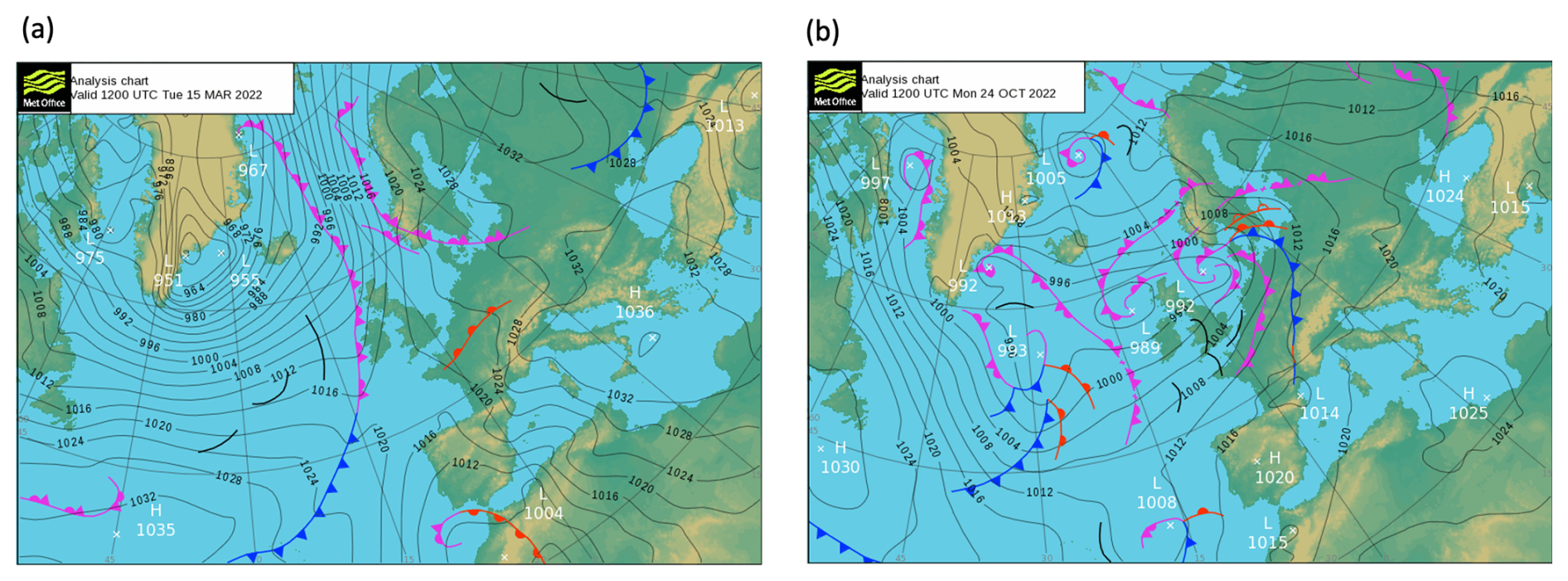
Figure 1 The UK Met Office surface analysis charts at 12:00 UTC on (a) 15 March 2022 and (b) 24 October 2022.

2.2 Model setup

The Met Office Unified Model (UM) (Brown et al., 2012) version 13.0 with the Regional Atmosphere and Land (RAL) 3.2 configuration (Bush et al., 2020, 2022) was used in this study. A 1500 km by 1500 km regional domain with 1.5 km grid spacing and centred at 59° N, 52° W was nested within a global model (N216, ≃60 km grid spacing near the mid-latitudes) with the Global Atmosphere and Land (GAL) 6.1 configuration (Walters et al., 2017). The nested model domains are shown in Appendix C. Using a 1.5 km grid spacing has shown a good ability to reproduce the general features of the CAO cloud system (e.g. the stratus and cumulus regions) from Field et al. (2017a). Such design of the regional domain balances sufficient coverage of the CAO cloud system and the computational cost. There were 70 vertical levels in the nested region up to 40 km (28 model levels below 3 km where most of the cloud is in both cases), and the time step was 60 s for the regional model. The lateral boundary was provided to the regional model from the global model every hour. The simulations were initialized from archived global model analysis at 00:00 UTC on the case date and run for 24 h. The first 12 h were excluded from the analysis due to model spin-up.

Cloud microphysics are parameterized with the double-moment bulk Cloud AeroSol Interacting Microphysics (CASIM) scheme (Shipway and Hill, 2012; Grosvenor et al., 2017; Field et al., 2023). There are five hydrometeor species in CASIM, i.e. cloud liquid, rain, cloud ice, snow, and graupel, with a generalized gamma distribution for the particle size distributions (PSDs). CASIM provides two options to calculate the droplet number concentration (N_d): prescribing a fixed in-cloud N_d or deriving N_d from the background aerosol. The prescribed fixed N_d option was selected in this study for an easier perturbation of N_d and interpretation of the results. However, it is worth noting that using fixed in-cloud N_d instead of having aerosols involved can remove potential feedbacks between aerosols and clouds; for example, precipitation formed in clouds can remove aerosols/CCNs, which can enhance the precipitation and further remove the aerosols. Details on the selection of parameter values are given in Sect. 2.3 below. For heterogeneous ice nucleation on INPs (primary ice production, PIP), we use the parameterization of Cooper (1986). The Cooper approach is a parameterization for the ice crystal number concentration (N_ice), but because we assume that one INP can produce one ice crystal, the Cooper approach is treated as an INP parameterization in this study. Heterogeneous ice nucleation is assumed to occur in grid boxes with temperatures lower than −8 °C – and higher than −38 °C when homogeneous ice nucleation can occur. Bigg's parameterization for rain freezing (Bigg, 1953) was switched off in this study to avoid potentially unrealistic formation of graupel in convective clouds. The secondary ice production (SIP) process implemented in CASIM is the Hallett–Mossop (HM) process (Hallett and Mossop, 1974), which produces ice splinters through riming between −2.5 and −7.5 °C, with a peak efficiency at −5 °C. The rates were calculated from cloud liquid accreted by graupel and snow with a default efficiency of 350 ice splinters produced per milligram of rimed cloud liquid. Other SIP mechanisms (e.g. collision fragmentation Vardiman, 1978; Takahashi et al., 1995 and droplet shattering Latham et al., 1961) are currently in development and hence not available for use in this study. When both ice and liquid existed in the same grid box, the overlap mixed-phase fraction was calculated, with a fixed mixed-phase overlap factor of 0.5 (Field et al., 2023). The mixed-phase overlap factor controls a function that quantifies the overlap during the run time of the model rather than being a fixed mixed-phase overlap in a model grid box. If the overlap factor is set to 1, then the subgrid liquid and ice cloud are maximally overlapped. If the overlap factor is 0, then the subgrid liquid and ice are not overlapped as long as ${\text{CF}}_{\text{liq}}+{\text{CF}}_{\text{ice}}<\mathrm{1}$, where CF refers to the cloud volume fraction. Once the combined cloud fraction goes above 1, there will be overlap. For an overlap factor of 0, the overlap is minimized. Values of the overlap factor in between lead to increasing overlap, but once either the liquid or ice cloud fraction reaches 1, then mixed-phase overlap is maximum regardless what the overlap factor is set to. See Sect. A.6 in the documentation of the CASIM implementation in UM from Field et al. (2023) for more information.

The cloud parameterization in the nested UM is a diagnostic cloud scheme that uses skewed and bimodal probability density functions for subgrid saturation departure. This bimodal cloud scheme diagnoses the cloud volume fractions and condensed liquid water amounts in each grid box and passes them to CASIM. It is the bimodal cloud scheme that handles the condensation and evaporation between water vapour and cloud liquid via a saturation adjustment approach justified by the long model time step (approx. 60 s) compared to the timescales of saturation adjustment (approx. 1 s). This process happens at a different point in the UM time step relative to the CASIM microphysics. A detailed technical explanation of coupling CASIM to the cloud schemes in UM is given in Field et al. (2023).

The radiative processes in the simulations are represented by SOCRATES (Suite Of Community Radiative Transfer codes based on Edwards and Slingo) (Edwards and Slingo, 1996; Manners et al., 2023), which calculates radiative fluxes using the two-stream method and radiance using spherical harmonics. The single-scattering properties of water droplets are dependent on the mass mixing ratio of liquid water and the effective radius of the droplets (Slingo and Schrecker, 1982). In this study, the single-scattering properties of ice crystals are calculated using an equivalent mass spherical radius with both the ice water mass mixing ratio and ice hydrometeor number concentration (N_ice) from CASIM. This allows a “Twomey-like” effect to be included from changes in N_ice.

2.3 Perturbed parameters and the selection of their values

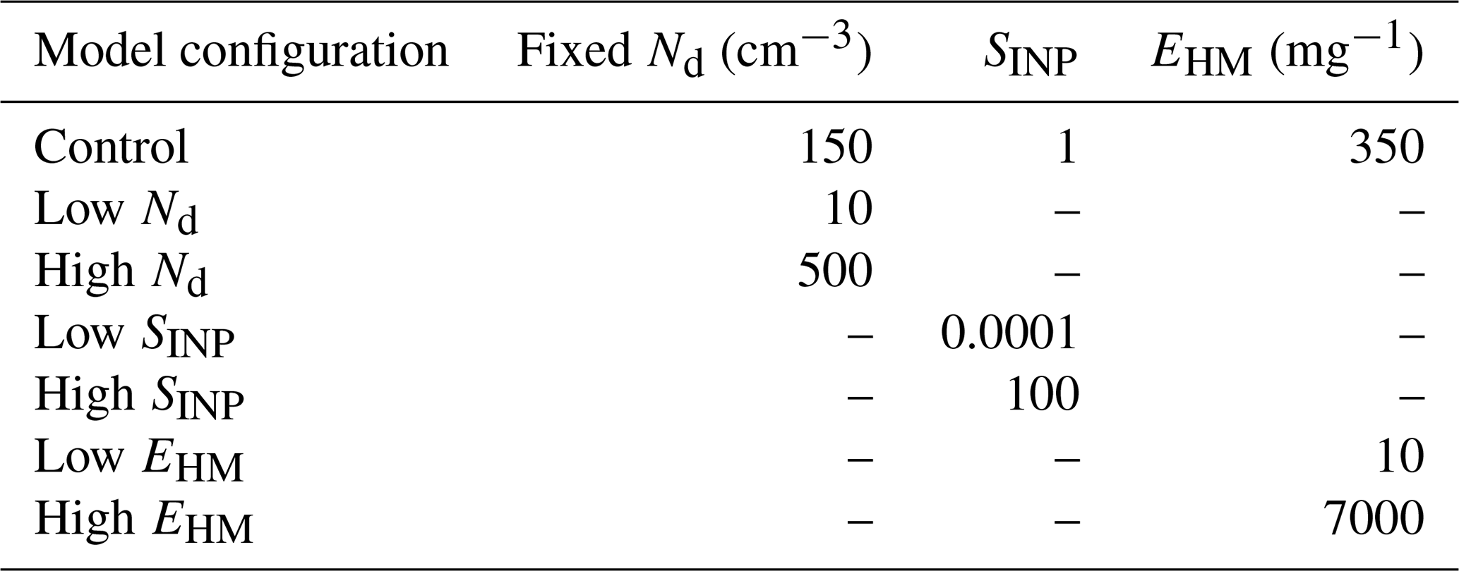
Three model input parameters are perturbed in this study: the prescribed fixed in-cloud droplet number concentration (N_d), the scale factor of the INP concentration (S_INP), and the ice multiplication efficiency of the Hallett–Mossop process (E_HM). Table 1 shows the values used for each simulation, and the selection of the parameter values is explained below.

Table 1 Configurations of simulations for both case studies. Cell content marked by “–” means that the value used for the parameter is the same as the configuration in the control simulation.

2.3.1 Droplet number concentration (N_d)

CASIM provides two options for calculating N_d. Here, we use fixed in-cloud N_d to allow an easier interpretation of the results instead of deriving N_d from the background aerosol. The grid-box mean N_d is calculated by multiplying the fixed in-cloud N_d with the liquid cloud fraction in the grid box from the bimodal cloud scheme. The default value of the fixed in-cloud N_d is 150 cm⁻³, and we selected 10 cm⁻³ for low N_d and 500 cm⁻³ for high N_d simulations based on values from Wood (2012) for general stratocumulus clouds. This range also covers the observations from the M-Phase measurements (Murray and the MPhase Team, 2024; Tarn et al., 2025) and warm cloud N_d derived from satellite retrievals (Grosvenor et al., 2018) in this region.

2.3.2 Scale factor of INP concentration (S_INP)

The INP parameterization used in this study is the default heterogeneous ice nucleation parameterization from Cooper (1986), assuming that one INP produces one ice crystal. Here, we use a scale factor S_INP (unitless) to change the INP concentration from the default Cooper parameterization:

$$\begin{array}{}\text{(1)}& {\displaystyle }{\displaystyle }{N}_{\text{INP}}\left(T\right)=S_{\text{INP}}\left(\mathrm{5}{\mathrm{e}}^{-\mathrm{0.304}(T_{\mathrm{0}}-T)}\right).\end{array}$$

The unit of N_INP(T) is m⁻³. The default value of S_INP is 1.0. T₀ is 273.15 K, and T is the ambient temperature (K). A temperature of 265.15 K (−8 °C) was chosen as the warmest condition for ice nucleation, meaning there are no INPs at temperatures higher than −8 °C. We selected 0.0001 for low S_INP and 100 for high S_INP simulations to cover the majority of INP measurements in high-latitude regions of the Northern Hemisphere (Fig. 2a) and the INP measurements from the M-Phase aircraft campaign (Fig. 2b, Murray and the MPhase Team, 2024; Tarn et al., 2025). There is also a parameter in the Cooper parameterization that defines the dependence of N_INP on temperature. Although it has been shown to be important for deep convective anvil cirrus (Hawker et al., 2021a, b), it plays a secondary role in the CAO clouds of interest here, as the CAO clouds are generally thin (Fletcher et al., 2016b) and the slope in the default Cooper approach matches reasonably well with most of the M-Phase measurements in Fig. 2b.

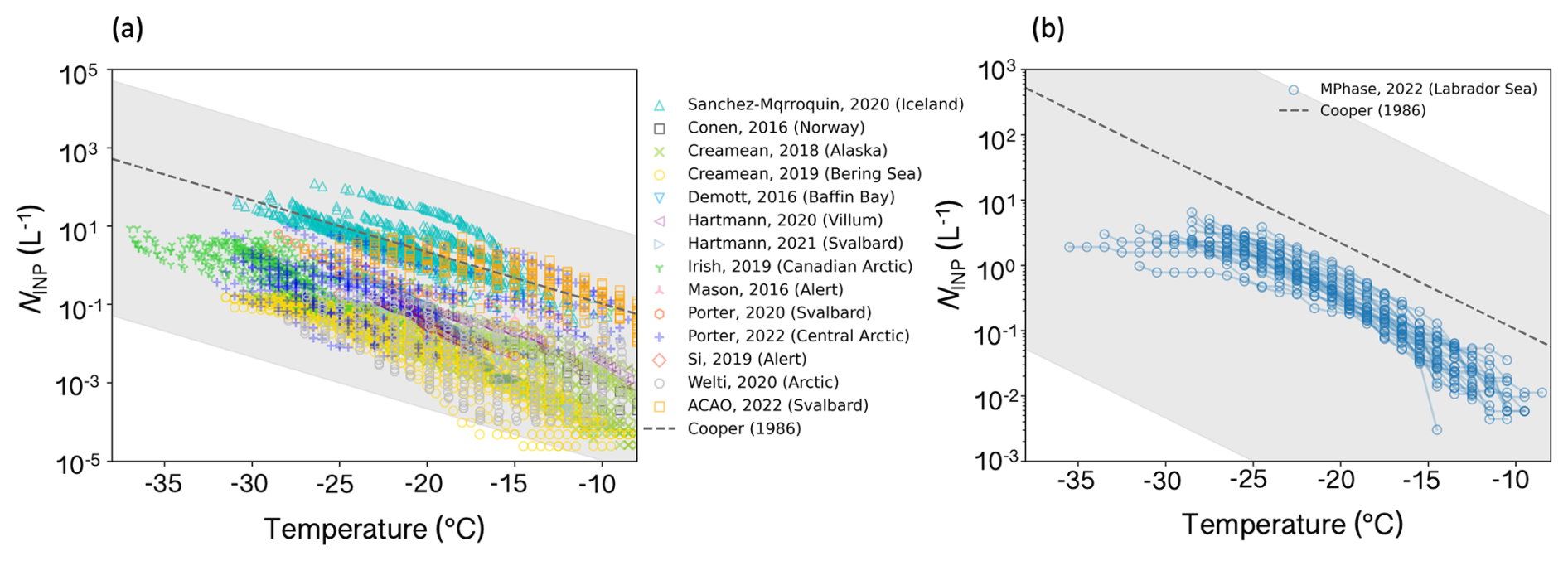
Figure 2 Perturbed INP range in this study compared to INP measurements in high-latitude regions in the Northern Hemisphere from (a) literature data (Sanchez-Marroquin et al., 2020; Conen et al., 2016; Creamean et al., 2018, 2019; DeMott et al., 2016; Hartmann et al., 2020, 2021; Irish et al., 2019; Mason et al., 2016; Porter et al., 2020, 2022; Si et al., 2019; Welti et al., 2020; Raif et al., 2024) and (b) the M-Phase aircraft campaign (Tarn et al., 2025). INP measurements from each flight during the M-Phase aircraft campaign are connected with lines to compare the INP concentration slope with the default Cooper parameterization slope. The top and bottom boundaries of the shaded area are the upper and lower perturbed range of the INP concentration in the sensitivity test.

2.3.3 Efficiency of the Hallett–Mossop process (E_HM)

The Hallett–Mossop (HM) process is included as the only SIP process in this study, with a default efficiency of 350 ice splinters produced per milligram of rimed cloud liquid (Hallett and Mossop, 1974; Field et al., 2023):

$$\begin{array}{}\text{(2)}& {\displaystyle }{\displaystyle }{P}_{\text{HM}}=E_{\text{HM}}(P_{\text{gacw}}+P_{\text{sacw}})f\left(T\right)M_{\text{I0}},\end{array}$$

where P_HM is the mass of ice produced from the HM process, E_HM is the HM process efficiency perturbed in this study, with a default value of 350 mg, P_gacw is the rate at which graupel accretes cloud water, P_sacw is the rate at which snow accretes cloud water, M_I0 is the produced splinter mass of 10⁻¹⁸ kg, and f(T) is a triangular function between −2.5 and −7.5 °C with a peak at −5 °C when f(T)=1. Clouds formed in the October case span this range of temperatures, while cloud temperatures in the March case are much colder, with few clouds formed in this range of temperatures (Sect. 3.1).

We selected 10 mg for low E_HM and 7000 mg for high E_HM simulations. The high E_HM value was selected following the studies by Young et al. (2019) and Sotiropoulou et al. (2020) to show good agreement with the observed N_ice when only the HM process is implemented in the model. The low E_HM was selected to test the effects of reducing the HM process but not completely removing it. It is worth noting here that self-limiting feedback may exist when using high E_HM (Field et al., 2017b), which can potentially limit the increase in ice splinters produced by increasing the E_HM through stronger removal of liquid for riming.

2.4 Satellite data

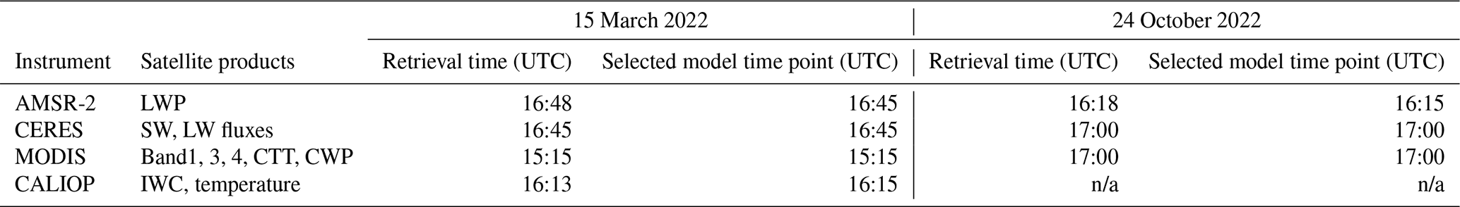
Multiple satellite data products were used in this study to compare the model output with observations. Figure 3 shows the satellite data products for the two CAO cases, including RGB composites (a and e) using bands 1 (620–670 nm), 3 (459–479 nm), and 4 (545–565 nm) from the MODIS (Moderate Resolution Imaging Spectroradiometer) Level 1B Calibrated Radiances Product (Collection 6.1) (MCST, 2017a); the single scanner footprint (SSF) of top-of-atmosphere shortwave flux ($F_{\text{SW}}^{\text{TOA}}$, b and f) and longwave flux ($F_{\text{LW}}^{\text{TOA}}$, c and g) from the CERES (Clouds and the Earth's Radiant Energy System) instrument (Edition 4A) (Su et al., 2015a, b); and the cloud top temperature (d and h) from the MODIS Atmosphere Level 2 Cloud Product (Collection 6.1) (Platnick et al., 2015). The all-sky liquid water path (LWP) with a 0.25° spatial resolution retrieved from the AMSR-2 (Advanced Microwave Scanning Radiometer) columnar cloud liquid water product (version 8.2) (Wentz et al., 2014) and the cloud water path (CWP) for both liquid and ice and cloud cover from the MODIS Atmosphere Level 2 Cloud Product (Collection 6.1) (Platnick et al., 2015) were also used for the model–observation comparison, as shown in the “Results” section below. A table of retrieval time and selected model time points for each satellite product is shown in Appendix A.

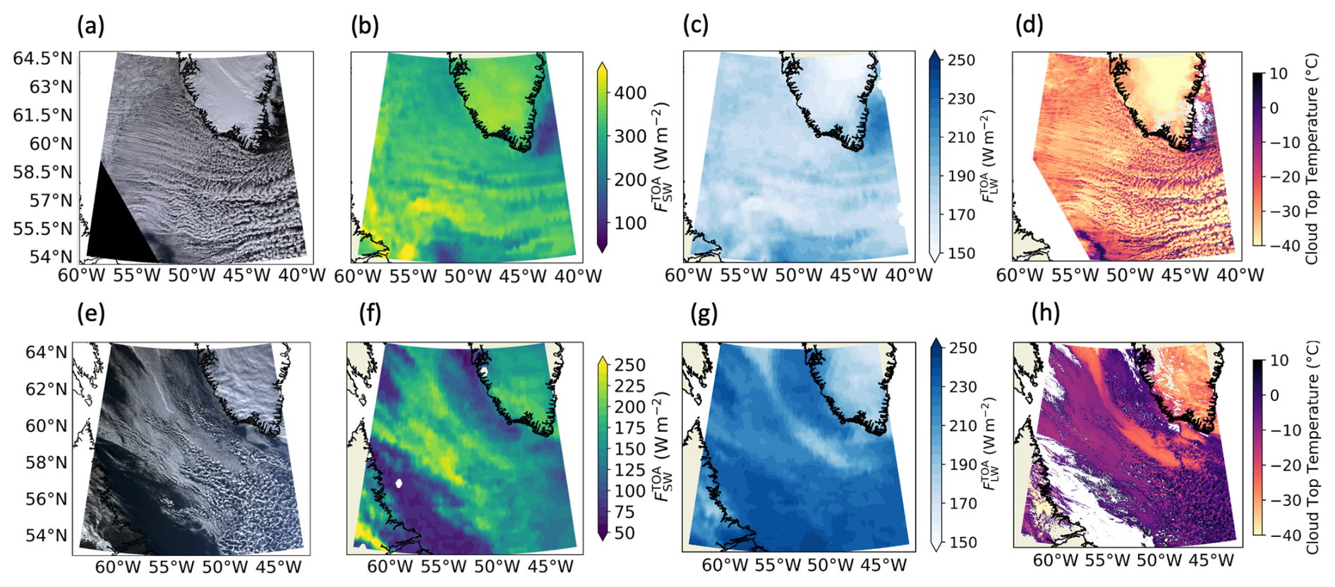
Figure 3 Satellite retrievals for CAO events over the Labrador Sea on 15 March 2022 (a–d) and 24 October 2022 (e–h): RGB imagery (a, e), top-of-atmosphere shortwave flux (b, f), top-of-atmosphere longwave flux (c, g), and cloud top temperature (d, h). Note that the scales of the colour bars for the shortwave radiation flux are different for these two cases due to different satellite retrieval times.

The MODIS and CERES instruments are on board NASA's Aqua satellite, and the AMSR-2 instrument is on board JAXA's (Japan Aerospace Exploration Agency) GCOM-W (Global Change Observation Mission – Water) satellite. Both polar-orbiting satellites have the same Equator crossing time of 13:30 UTC while ascending and similar altitudes for their orbits. This means satellite retrievals can be made close to each other in time. Geostationary satellite products are not used in this study due to large uncertainties in retrievals for high-latitude regions (Seethala and Horváth, 2010).

Although the two selected CAO events shared similar synoptic situations as shown in Fig. 1, their cloud top temperatures were very different. The March case had much colder cloud top temperatures with a peak around −30 °C, compared to the ones in the October case with a peak around −10 °C. Monthly distributions for cloud top temperature of low-level, mixed-phase clouds during CAO events over the Labrador Sea in 2022 are shown in Appendix B using the ERA5 (ECMWF ReAnalysis version 5) (Hersbach et al., 2020) dataset and CTT retrieved from MODIS. The CTTs in the March case are near the colder end of the shown distributions, while the ones in the October case are more close to the warmer end, which suggests that these two CAO cases nicely contrast with each other in terms of CTTs and sit near the boundaries of CTT ranges in CAO clouds over the Labrador Sea. These two cases were chosen on the basis that they represent end members of the temperature range of mixed-phase CAO clouds. Detailed information regarding the method of analysis is shown in Appendix B.

3 Results

3.1 Control simulations

Control simulations with the default model setup are introduced and compared in this section. Figure 4 shows the modelled in-cloud cloud water path (CWP), which is the sum of the in-cloud liquid water path (LWP) and the in-cloud ice water path (IWP), for both cases compared with the MODIS-retrieved in-cloud CWP. This comparison acts as a qualitative check of whether our model can simulate the main synoptic features of the CAO cloud system. The MODIS-retrieved CWP data were regridded to the same spatial resolution as the modelled CWP (1.5 km) using the nearest-neighbour method. The satellite retrieval time and selected model output time point are shown in Appendix A.

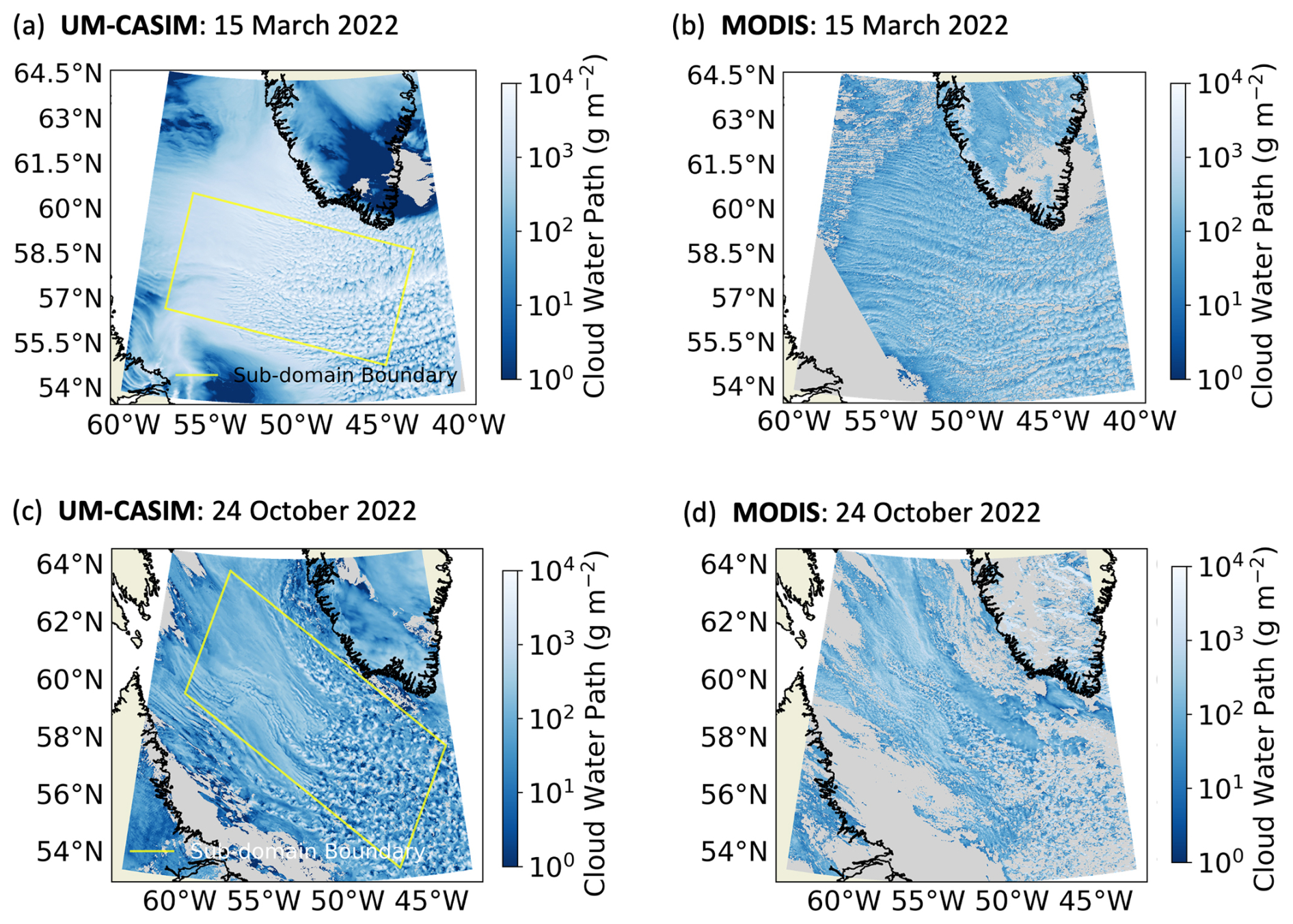
Figure 4 In-cloud cloud water path (CWP) from the control UM-CASIM simulations and MODIS retrievals on 15 March 2022 (a, b) and 24 October 2022 (c, d). The model reproduces the general CAO cloud system in both case studies well when compared to satellite retrievals. The in-cloud cloud water path retrieved from MODIS is not used for a quantitative comparison due to its large uncertainties. Sub-domains of interest for both cases are highlighted in yellow. Model output pixels with less than 20 % cloud cover are excluded before calculating the in-cloud values. Times of model output and satellite retrieval are shown in Appendix A.

In general, the March CAO event has a less broken cloud field with higher CWP compared to the October CAO event. For both cases, the control simulations capture the cloud regimes (e.g. stratus and open cells) during the CAO event and reproduce the large-scale synoptic structures and the locations of the CAO event well compared with the MODIS retrievals. In the March case, the model struggles with reproducing the fine structures of cloud streets to the east of 54° W in the sub-domain. This is because the effective horizontal resolution (between 5 and 10 times the grid spacing) in our model cannot fully resolve the cloud streets at the beginning of the CAO event. With the clouds moving into the convective region and the boundary layer becoming deeper (to the west of 54° W), the scales of the cloud street grow and can then be resolved in the model. A better representation of the cloud streets at the beginning of the CAO event requires higher model resolution (Field et al., 2017a) and therefore much higher computational resources to conduct the sensitivity test; hence, they are not further investigated here. Our control simulations generally have higher in-cloud CWP compared with the MODIS retrieval, which may be because of the different definitions of cloudy pixels between the model output and satellite products, uncertainties in the MODIS-retrieved CWP for high-latitude mixed-phase clouds (Khanal and Wang, 2018), and potential overestimation of the CWP from our model.

Note that the CWP comparison is only qualitative here, and quantitative model–observation comparisons of the control simulations with satellite retrievals of cloud top temperature from MODIS, temperature and IWC (ice water content) from CALIOP for the March case, and M-Phase aircraft measurements of temperature, cloud water content, and liquid water fraction for the October case are shown and discussed in Appendix D. Quantitative comparisons of all-sky LWP, shortwave (SW) fluxes, and longwave (LW) fluxes between the model output from all simulations (control and sensitivity test simulations) and satellite retrievals are shown later in Sect. 3.5.

Cross-section mean cloud properties within the highlighted sub-domain (yellow parallelogram) in Fig. 4 of both cases are presented and compared in Fig. 5, with supplementary information shown in Appendix E. The sub-domain was selected to be aligned with the directions of wind and cloud movements, and the cross-section mean was calculated by averaging along the y axis of the sub-domain parallelogram. The locations of the sub-domains in the nested model domains are shown in Appendix C. The whole sub-domain in the March case and most of the sub-domain (except the small northwestern part) of the October case are sufficiently distant from the boundaries of the nested model domain and hence not affected by the boundary effects from fields entering from the global model. A detailed discussion on the boundary effects is given in Appendix C.

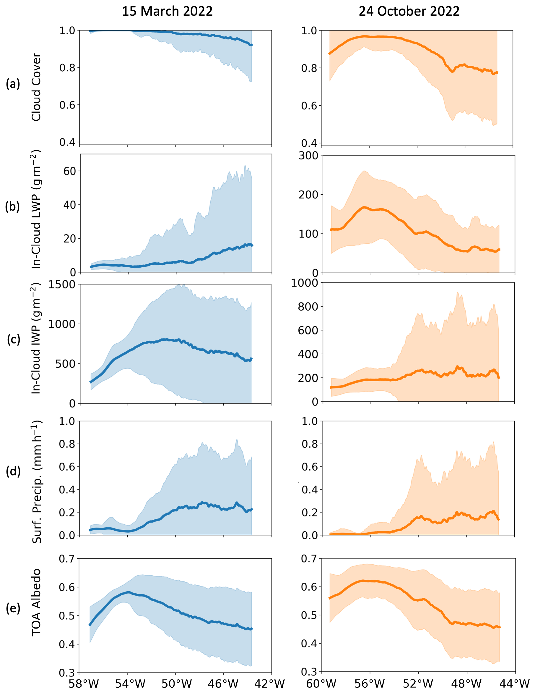
Figure 5 Cross-section mean (averaging along y axis of the sub-domain parallelogram shown in Fig. 4) cloud properties from the March (left panel) and October (right panel) control simulations: (a) cloud cover, (b) in-cloud liquid water path (LWP), (c) in-cloud ice water path (IWP), (d) surface precipitation, and (e) albedo at the top of the atmosphere (TOA albedo). The time points selected are 16:45 UTC for the March case and 17:00 UTC for the October case, which are consistent with the corresponding CERES measurement times. Grid boxes with cloud cover smaller than 20 % were removed before averaging for calculation of the in-cloud LWP and in-cloud IWP. The shaded area indicates the range of ±1 standard deviation.

Both cases experience a general west-to-east reducing trend of cloud cover (Fig. 5a) in the sub-domain along the direction of cloud movements to the open ocean, with the March case having a generally higher cloud cover (>0.9 for most of the cross-section) compared to the one in October. The in-cloud LWP (Fig. 5b) is much higher in October, with the peak LWP happening around 150 g m⁻² near 56° W in October and less than 20 g m⁻² near the eastern boundary of the sub-domain in March. The trend of LWP changing from the west to the east of the sub-domain is different in these two cases: a general increasing trend in March and a trend wherein the LWP first increases to the peak value and then reduces in October. The in-cloud IWP (Fig. 5c) is much higher in the March case, with the peak around 750 g m⁻² near 50° W. The in-cloud IWP starts at a low level in October and generally increases from west to east, with the peak value slightly lower than 300 g m⁻² near the eastern boundary of the sub-domain. The liquid water fraction, the ratio of LWP to CWP, is calculated to show the liquid–ice partitioning in both cases (Appendix E). The dominant cloud water is in the ice phase in the March case, whereas the liquid phase dominates in the western region in October, after which the ice phase dominates when clouds move towards the east. Both cases experience little precipitation in the western region and enhanced precipitation when clouds move further east (Fig. 5d), with the dominant type of precipitation being snow in March and rain in October (Appendix E).

As the SW radiation dominates cloud radiative effects in shallow mixed-phase clouds, we use albedo at the top of the atmosphere (TOA) in Fig. 5e to investigate the CAO cloud radiative properties. The outgoing shortwave and longwave fluxes are shown in Appendix E. The overall trend of the albedo changing from the west to the east of the sub-domain is very similar in these two cases, with the albedo slightly higher in October. By comparing the trend with the other cloud properties mentioned above, it is shown that albedo is strongly affected by the cloud cover in both cases but influenced more from in-cloud IWP in March and more from in-cloud LWP in October. This is due to the variation of the liquid–ice partitioning in their control simulations and the fact that the liquid–ice partitioning is strongly controlled by the cloud temperature, with the same temperature-dependent INP parameterization (as well N_d and E_HM). The cross-section mean values for cloud profiles (cloud volume fraction and total water content) with ambient temperature are shown in Appendix E. Most of the clouds in the March case in the sub-domain are between −15 and −35 °C, while the ones in the October case, having a much warmer ambient temperature, are mostly between 0 and −15 °C. Such temperature difference can directly lead to different efficiencies of many temperature-dependent cloud microphysics processes, including the INP concentration and HM efficiency perturbed in this study during these two cases.

The meteorological variables and environmental conditions of the boundary layer are also shown and compared for the control simulations of these cases in Fig. E2 of Appendix E. The SST (sea surface temperature) increases as clouds move eastward, with the SST lower in the March case (2–3 °C) than in the October case (4–7 °C). Note that the SST was prescribed based on daily forecasting analyses in all our model simulations. The March case is a much stronger CAO event, with the highest CAO index at 800 hPa (M₈₀₀), almost reaching 20 K at the western boundary of the sub-domain, whereas the highest M₈₀₀ is around 1.5 K in the October case. The more unstable boundary layer in the March case is consistent with a lower LTS (lower tropospheric stability) compared to the one in the October case. Both cases experience an EIS (estimated inversion strength) over 5 K at the western boundary of their sub-domain, with a decreasing trend to the east.

3.2 Responses of cloud properties to perturbed parameters

In this section, the responses of the cloud properties to the perturbations in droplet number concentration (N_d), the INP concentration (S_INP), and the efficiency of the HM process (E_HM) are compared between the two cases. An overall comparison between the two cases and the cloud profiles is given later in Sect. 3.4.

3.2.1 15 March 2022

Here, we first present the responses of cloud cover, in-cloud LWP, in-cloud IWP, surface precipitation rate, and TOA albedo in Fig. 6 for the March case, as well as the other properties shown in Appendix F (Fig. F1). There is limited influence from perturbing N_d (left panel) and E_HM (right panel) on the cloud properties in March. The effects from these parameters are small due to little water in the control simulation and most clouds being out of the active temperature range for the HM process in March, as shown in Fig. E3 of Appendix E.

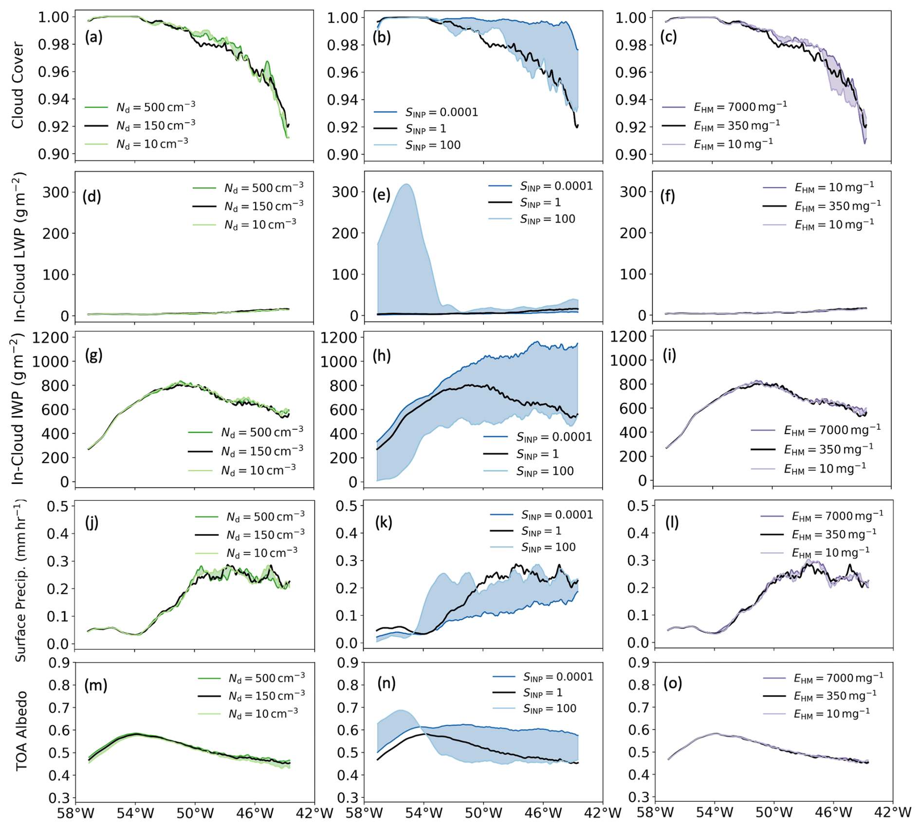
Figure 6 Responses of cross-section mean CAO cloud properties to the three perturbed parameters on 15 March 2022 at 16:45 UTC: (a–c) cloud cover, (d–f) in-cloud liquid water path (LWP), (g–i) in-cloud ice water path (IWP), (j–i) surface precipitation, and (m–o) albedo at the top of the atmosphere (TOA albedo). Grid boxes with cloud cover smaller than 20 % were removed before calculating in-cloud LWP and IWP. The time of 16:45 UTC was chosen for the corresponding CERES measurements of radiation on 15 March 2022. The space between the variable data from the high and low simulations is filled to highlight the range of variables and identify non-monotonic behaviours (e.g. data from the control simulation are not in the shaded space).

Perturbing S_INP (middle column of panels) has a much stronger influence on all the column cloud properties shown here than perturbing N_d or E_HM. With a higher INP concentration, the modelled CAO clouds experience a higher cloud cover from around 54° W to the eastern boundary of the sub-domain and a higher in-cloud IWP throughout the sub-domain (stronger increase in the eastern region) along with less surface precipitation. The in-cloud LWP decreases only slightly because there is so little liquid water in the control simulation, with a similar change for the liquid cloud fraction (Appendix E). The limited influence from lower in-cloud LWP is then offset by the higher cloud cover and higher in-cloud IWP, resulting in a general higher TOA albedo in the high INP concentration simulation.

The responses of in-cloud LWP, IWP, and liquid water fraction are consistent with previous studies (Abel et al., 2017; Tornow et al., 2021), but the responses of cloud cover, surface precipitation, and TOA albedo differ from the previous studies, where the CAO cloud cover becomes smaller with a higher INP concentration (Tornow et al., 2021). Similarly, Abel et al. (2017) found that cloud cover increased when they prevented ice formation. In this March case, the increase in cloud cover with higher INP concentration is due to the small amount of liquid water in the control simulation such that the increase in ice concentrations has only a small effect on the further removal of liquid water. In addition, with a higher INP concentration, there is a higher ice number concentration, and the autoconversion from ice crystals to snow becomes slower; moreover, the mean ice hydrometeor particle size becomes smaller, resulting in a lower mean fall speed and reduced sedimentation flux. These effects lead to less precipitation and slower removal of cloud water, resulting in greater cloud cover. The responses here to a higher INP concentration are similar to what we would expect in cirrus clouds.

With a lower INP concentration, a strong increase in the in-cloud LWP is seen in the western sub-domain, with the peak value over 300 g m⁻². However, a sharp reduction of in-cloud LWP follows around 53–52° W, as well as strong surface precipitation at the same location. This strong removal of liquid water from clouds limits the influence of decreasing INP on increasing the in-cloud LWP in the rest of the sub-domain. Compared to the control simulation, lower INP concentration has limited influence on the cloud cover and leads to a generally lower in-cloud IWP throughout the sub-domain. The change in TOA albedo is slightly complex: in the western sub-domain, before the liquid water is rapidly removed, a higher albedo is seen because of the much higher LWP; after the strong removal of LWP, the albedo reduces quickly and becomes lower than the one in the control simulation, which is a result of the lower in-cloud IWP. While the enhanced reflectivity with decreased INP is confined to the beginning of the sub-domain, the response to INP in the rest of the sub-domain extends over a massive area stretching out into the Atlantic and dominates the radiative effect of the INP over the sub-domain region as a whole.

3.2.2 24 October 2022

A similar analysis for the October CAO case is shown in both Fig. 7 and Appendix F (Fig. F2). Unlike the March case, where only the S_INP simulation strongly influences the cloud properties, all three perturbed parameters show clear and various influences in this October case, and some responses of cloud properties vary in the CAO development from west to east.

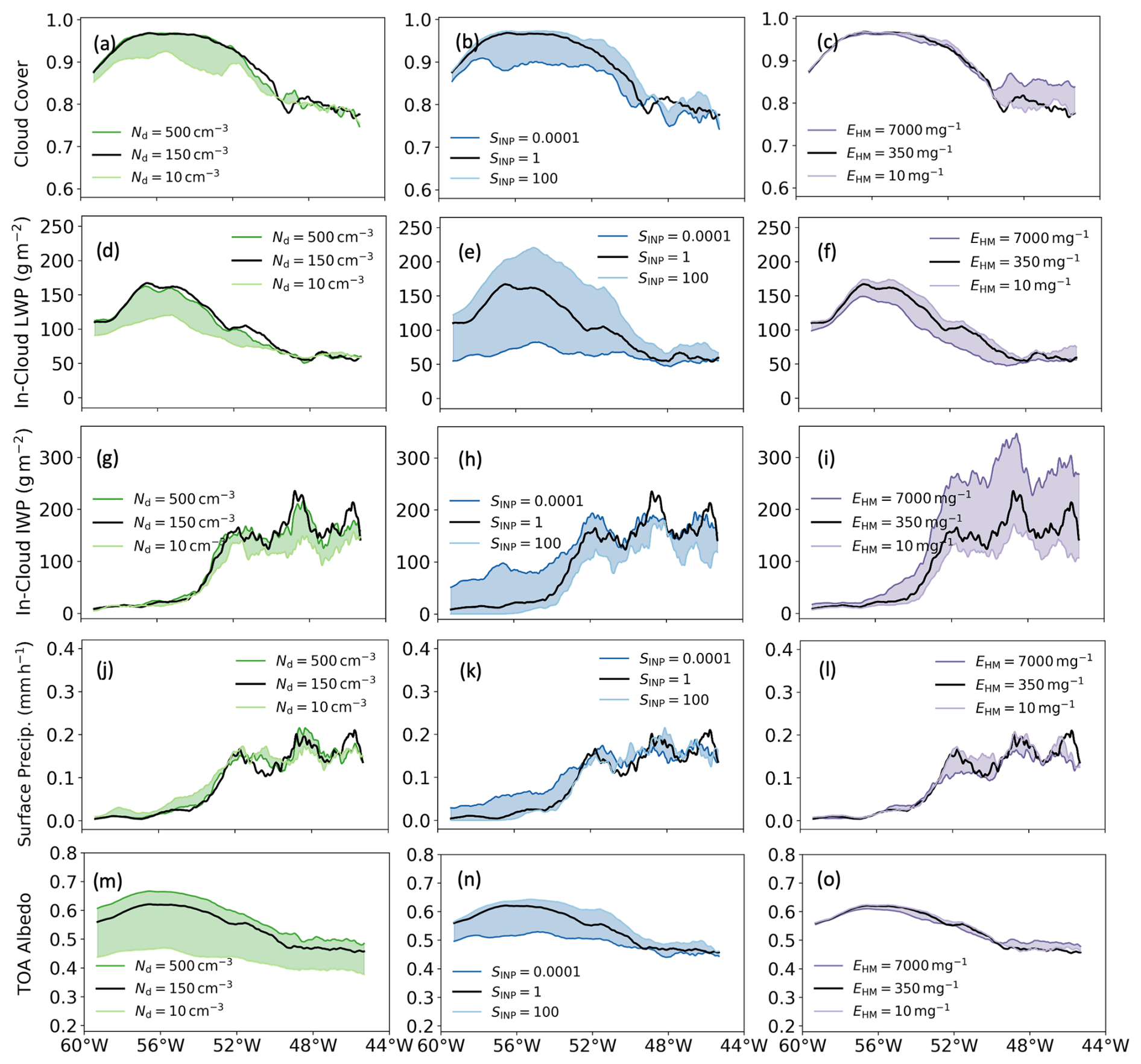
Figure 7 Responses of cross-section mean CAO cloud properties to the three perturbed parameters on 24 October 2022 at 17:00 UTC: (a–c) cloud cover, (d–f) in-cloud liquid water path (LWP), (g–i) in-cloud ice water path (IWP), (j–i) surface precipitation, and (m–o) albedo at the top of the atmosphere (TOA albedo). Grid boxes with cloud cover smaller than 20 % were removed before calculating in-cloud LWP and IWP. The time of 17:00 UTC was chosen for the corresponding CERES measurements of radiation on 24 October 2022. The space between the variable data from the high and low simulations is filled to highlight the range of variables and identify non-monotonic behaviours (e.g. data from the control simulation are not in the shaded space).

Perturbing N_d now has a strong influence on CAO cloud cover, in-cloud LWP, and TOA albedo in this October case. A low N_d leads to lower cloud cover and LWP along with higher surface precipitation, which is consistent with the Albrecht effect (Albrecht, 1989). With a high N_d, there is limited influence on cloud cover at the beginning of the CAO cloud system, as the precipitation rate is very small in the control simulation at this location and hence cannot be further suppressed with a higher N_d. The responses of the TOA albedo to both low and high N_d are the strongest among all the sensitivity test simulations in October, consistent with the Twomey effect (Twomey, 1977).

The responses of cloud properties to the perturbation of S_INP from the western boundary to around 50° W are similar to the CAO cloud responses to INP concentration or ice in previous studies (Abel et al., 2017; Tornow et al., 2021). The responses become complex and even become non-monotonic in some cases near the eastern end of the sub-domain. Until around 50° W, a higher INP concentration results in lower cloud cover, in-cloud LWP, and TOA albedo and higher in-cloud IWP and surface precipitation, and vice versa.

Various responses of cloud properties are also seen when perturbing E_HM. With a high E_HM, which means a more efficient HM process in the simulation, the cloud cover, surface precipitation, and TOA albedo are only affected strongly close to the eastern end of the sub-domain. This is because the HM process in the model is dependent on the processes of cloud water accretion onto graupel and snow, while ice is very limited in the stratocumulus-dominated region, but a higher IWP is seen after SCT. A high E_HM leads to higher cloud cover, a lower surface precipitation rate, and a higher TOA albedo. This is because although the HM process is the source of ice crystals, it is also the sink for graupel and snow, which can accrete and remove water through precipitation in the model. A high E_HM results in a lower amount of graupel and snow, hence leading to less precipitation. The responses of in-cloud LWP and in-cloud IWP are consistent throughout the sub-domain, with a high E_HM resulting in lower in-cloud LWP (through riming) and higher in-cloud IWP (slow snow autoconversion with a high ice crystal number concentration). These influences become stronger in the eastern region. Although low E_HM has a limited influence compared to high E_HM, one might notice that the responses of surface precipitation to E_HM become complicated and non-monotonic (e.g. the default model output is outside the low and high ends of the model output range) near the end of the sub-domain, where cumulus clouds dominate. For example, low E_HM results in stronger surface precipitation from 52 to 50° W but weaker surface precipitation around 46° W, compared to the precipitation from the control simulation. This may occur because the precipitation rate is a state-dependent variable and a low E_HM leads to an earlier peak of precipitation when clouds move eastward compared to the peak from the control simulation, followed by a lower precipitation rate later as less cloud water exists.

3.3 Responses of CAO cloud field development to perturbed parameters

Cloud field development, including the stratocumulus-to-cumulus transition (SCT), is important for the radiative properties of CAO clouds. In this section, we use the cloud field homogeneity parameter (ν) calculated using the in-cloud cloud water path (CWP), which has been successfully used for identifying cloud field transitions from satellite retrievals (Wood, 2012; Wu and Ovchinnikov, 2022), to understand how the perturbed parameters affect the cloud field development in the two selected cases. The cloud field homogeneity parameter (ν) is calculated using the squared ratio of the mean ($\overline{x}$) to the standard deviation (σ) for CWP over 20 by 20 grids: $\mathit{\nu }=(\frac{\overline{x}}{\mathit{\sigma }}{)}^{\mathrm{2}}$.

Figures shown in this section are the cross-section mean of the cloud field homogeneity parameter in the selected sub-domain. A sharp decrease in the cloud field homogeneity parameter generally implies a transition from stratocumulus clouds (Sc) to cumulus clouds (Cu). We also qualitatively determine the stratocumulus-dominated, transition, and cumulus-dominated regions by using the trends of the cloud field homogeneity parameter and the fraction of the 20 by 20 grids that are of the cumulus-capped boundary layer type. The methods for determining the boundary layer type in the UM are shown in Lock (2001). A quantitative determination of where the transition happens is not conducted in this study and requires further research on using the cloud field homogeneity parameter for model output. Note that we did not define the regions for different simulations individually to avoid any location effects. A detailed description of how we qualitatively define these regions can be found in the captions of Figs. 8 and 9.

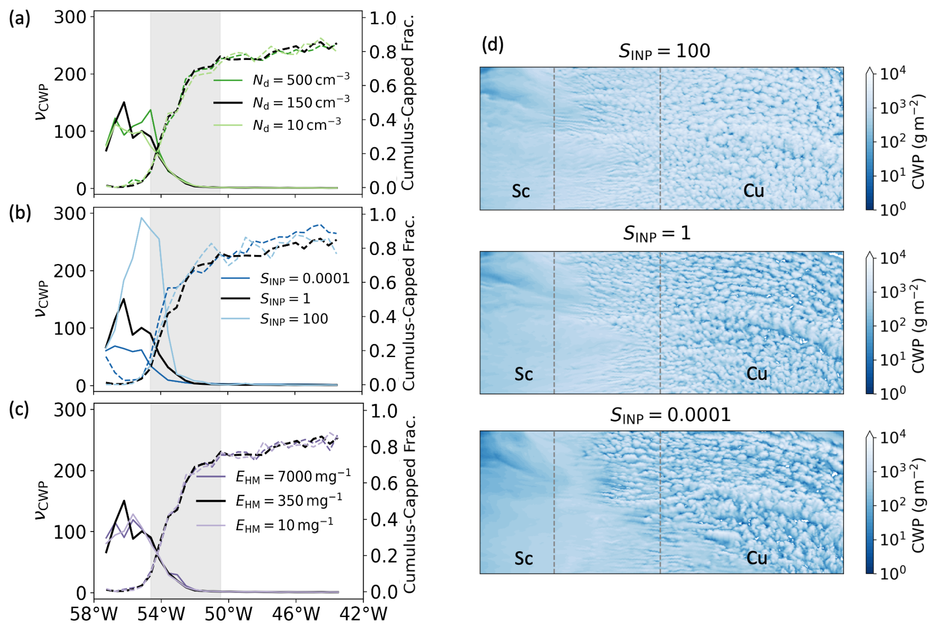
Figure 8 The cloud field homogeneity parameter (ν, solid lines) and the fraction of cumulus-capped boundary layer (dashed lines) in cloudy pixels (cloud cover ≥20 %) for simulations with perturbed N_d (a), S_INP (b), and E_HM (c) on 15 March 2022; (d) shows the 2D fields of the cloud water path for simulations with perturbed S_INP. Grey-shaded areas in (a–c) and the region between the grey dashed lines in (d) are the general stratocumulus-to-cumulus transition regions selected using both the cloud field homogeneity parameter (ν) and the fraction of cumulus-topped boundary layer. Note that we did not define the regions for different simulations individually to avoid any location effects. The stratocumulus-dominated region is determined to be located before the sharp decrease in the cloud homogeneity parameter and before the sharp increase in cumulus-capped boundary layer fraction; the cumulus-dominated region is determined to be where both the cloud homogeneity parameter and the cumulus-capped boundary layer fraction become stable; and the rest is determined as the transition region.

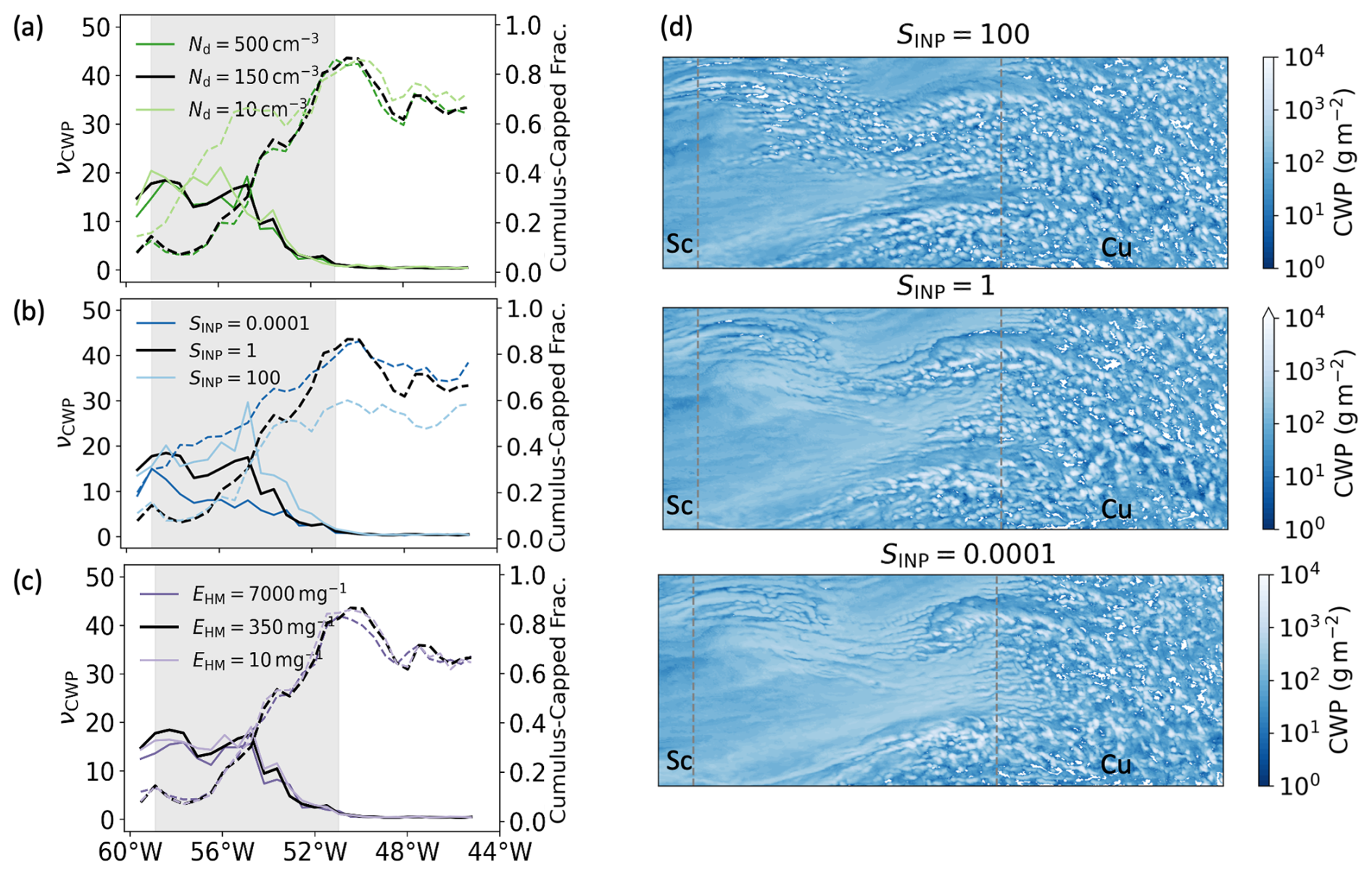
Figure 9 The cloud field homogeneity parameter (ν, solid lines) and the fraction of cumulus-capped boundary layer (dashed lines) in cloudy pixels (cloud cover ≥20 %) for simulations with perturbed N_d (a), S_INP (b), and E_HM (c) on 24 October 2022; (d) shows the 2D fields of the cloud water path for simulations with perturbed S_INP. Grey-shaded areas in (a)–(d) and the region between the grey dashed lines are the general stratocumulus-to-cumulus transition regions selected using both the cloud field homogeneity parameter (ν) and the fraction of cumulus-topped boundary layer. Note that we did not define the regions for different simulations individually to avoid the location effect. The stratocumulus-dominated region is determined as that before the sharp decrease in the cloud homogeneity parameter and the sharp increase in cumulus-capped boundary layer fraction; the cumulus-dominated region is determined to be where the trend of the cloud homogeneity parameter and the overall cumulus-capped boundary layer fraction becomes stable; and the rest is determined as the transition region.

Figure 8 shows the evolution of the cloud morphology (in terms of the spatial distribution of CWP) together with the homogeneity parameter and the cumulus-capped boundary layer fraction in the March case. The contribution of other boundary layer types for all the simulations is shown in Appendix G. Figure 8d shows the CWP field with different S_INP, and the stratocumulus-dominated, transition, and cumulus-dominated regions are separated by grey dashed lines.

Similar to the cloud properties shown in Fig. 6, the overall development of the cloud field in March is only strongly influenced by S_INP. With a higher INP concentration, the CAO cloud field begins with a more heterogeneous stratocumulus-dominated region, a higher cumulus-capped boundary layer fraction, and a slightly earlier transition to a cumulus-dominated region, indicated by an earlier sharp decrease in the cloud field homogeneity parameter and increase in the cumulus-capped boundary layer fraction.

To test whether the effect of INP on cloud field homogeneity and boundary layer types is caused by modifications to precipitation through the precipitation-induced SCT mechanism from Abel et al. (2017), we performed additional simulations in which either precipitation or both evaporation and sublimation of precipitation were turned off, as well as a simulation without precipitation, evaporation, or sublimation (denoted as “no-all”), as shown in Appendix H1 and H2. Most of the difference in cloud field development is removed in the “no-precipitation” and “no-all” simulations, with limited influence from the “no-evaporation-and-sublimation” simulations. This shows that the influence of INP on the March case's cloud field morphology and boundary layer structure is mainly through precipitation evolution, which acts as a sink of moisture from the cloud layer.

Figure 9 shows a similar analysis for the October case. Compared to the cloud field in the March case above, the CAO cloud field in the October case is more heterogeneous, and the cumulus clouds begin to appear even at the western boundary of the sub-domain (Appendix G). Perturbing both N_d and S_INP now has strong influences on the cloud field. Despite the dependence of cloud properties on E_HM in the October case discussed above (Fig. 7), there are limited effects on the cloud field development from perturbing E_HM.

With a higher S_INP, the October CAO cloud field also has an earlier transition to a cumulus-dominated region, a more heterogeneous cloud field across all of the CAO domain, and a higher surface precipitation rate (shown in Fig. 7k). An earlier transition to a cumulus-dominated region is also seen with low N_d in the October case. Both high S_INP and low N_d simulations experience earlier and more intense precipitation at the early stage of the CAO cloud shown in Fig. 7, and this is consistent with the precipitation-induced SCT mechanism in CAO clouds from Abel et al. (2017). Such influence of low N_d on SCT is not seen in the March case, as there is limited influence of changing N_d on precipitation due to the very limited amount of liquid cloud in the control simulation. Note that the stratocumulus-dominated region in the October case is very limited here due to the cumulus clouds starting to show up at a very early stage of the sub-domain.

Several other factors may influence SCT during CAO events, but they were not examined in this study. These include sea surface temperature (SST), which can impact convection and turbulence; boundary layer stability; inversion layer strength; and humidity. Additionally, this work focused on only three cloud microphysics parameters, whereas other microphysical processes could also potentially affect SCT. Future research should aim to explore the influence of these additional factors to gain a more comprehensive understanding of factors controlling SCT in CAO events.

The regions identified here are used for the overall comparison of cloud properties in the sub-domain and in different regions between the March and October cases in the next section.

3.4 Overall comparison of the cloud responses to perturbed parameters between the cases

In this section, the responses of cloud properties are compared in terms of the fractional change relative to the default simulation (Fig. 10). We compared the fractional changes between the stratocumulus-dominated region (Fig. 10a), the cumulus-dominated region (Fig. 10b), and the overall domain, which includes the previous two regions and the transition region (Fig. 10c). Mean cloud profiles (grid-box with in-cloud total water content $>{\mathrm{10}}^{-\mathrm{6}}$ kg kg⁻¹) for the stratocumulus-dominated region and the cumulus-dominated region for each case are shown in Figs. 11 and 12 to illustrate the responses of in-cloud properties to the perturbed S_INP. The responses of in-cloud properties to N_d and E_HM are shown in Appendix I and will not be further discussed in detail here.

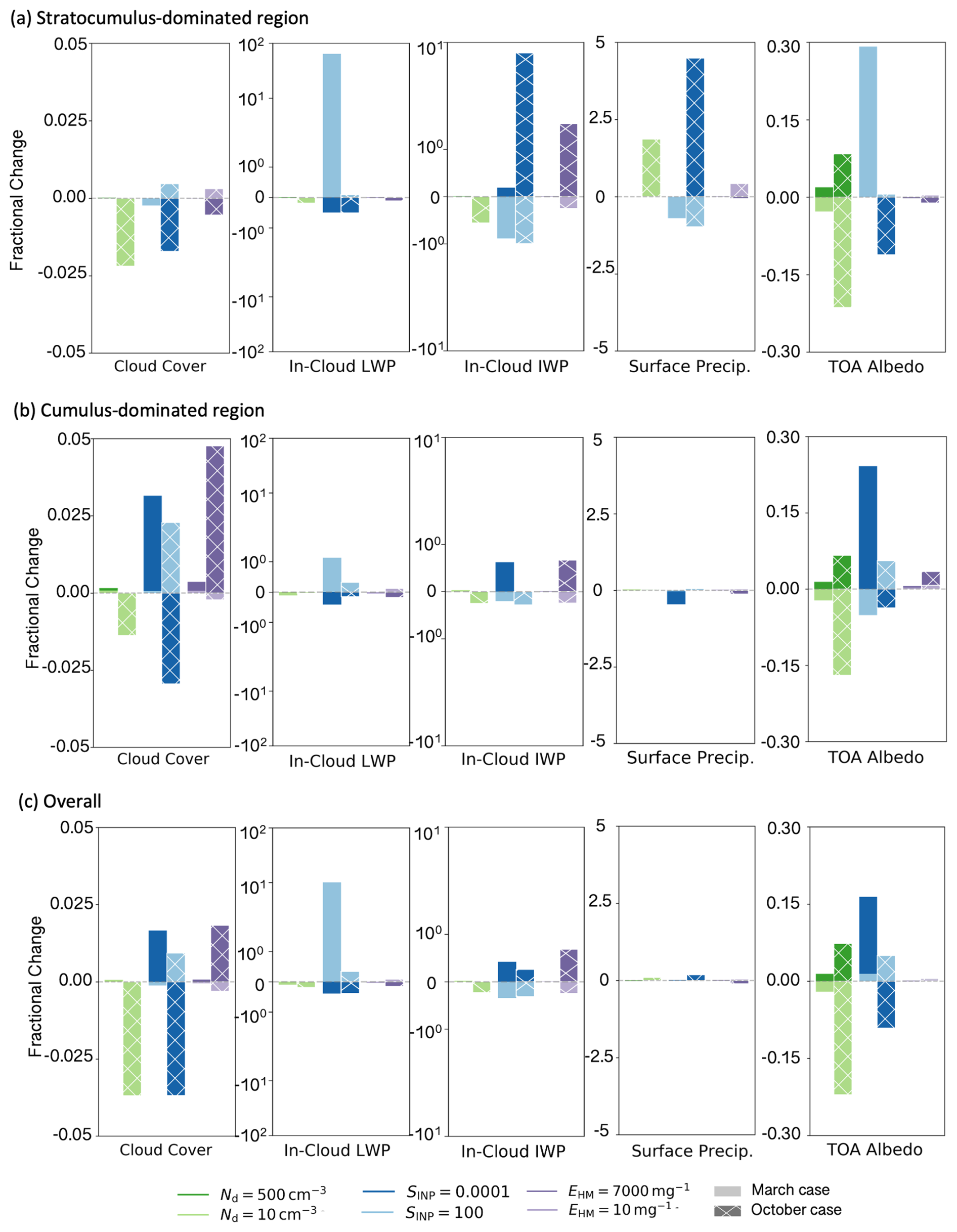
Figure 10 Fractional changes of cloud properties in the perturbed parameter simulations relative to the control simulations for the 15 March 2022 (solid shading) and the 24 October 2022 (hatched shading) cases, separated into the (a) stratocumulus-dominated domain, (b) cumulus-dominated domain, and (c) overall domain. Cross-section means of the sub-domain are shown in Figs. 6 and 7, and the determination of stratocumulus- and cumulus-dominated domains is discussed in Sect. 3.3. Note that the fractional change in the sub-domain is not just influenced by the fraction changes in the stratocumulus-dominated and cumulus-dominated regions but also by the proportion of each region.

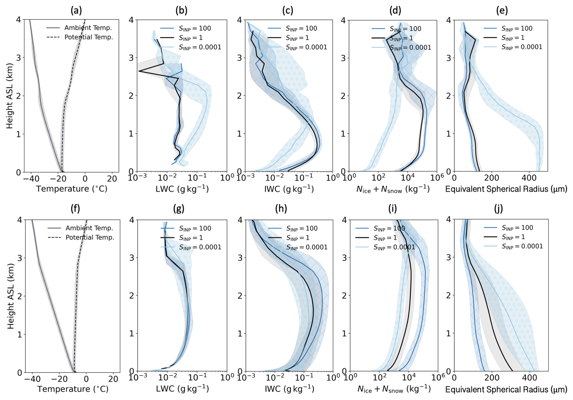
Figure 11 Vertical profiles for in-cloud properties in the March case: ambient temperature (default configuration), potential temperature (default configuration), in-cloud liquid water content (LWC), in-cloud ice water content (IWC), N_ice+N_snow, and equivalent spherical radius for stratocumulus-dominated (a–e) and cumulus-dominated (f–j) regions in the 15 March 2022 CAO case with different S_INP. The solid lines are medians, and the shaded areas are values between the 25 % quantile and 75 % quantile. For the cloud properties plots, grids with less than 10⁻⁶ kg kg⁻¹ total water content are removed. For hydrometeor number concentrations, cloudy grids with less than 1 m⁻³ are removed.

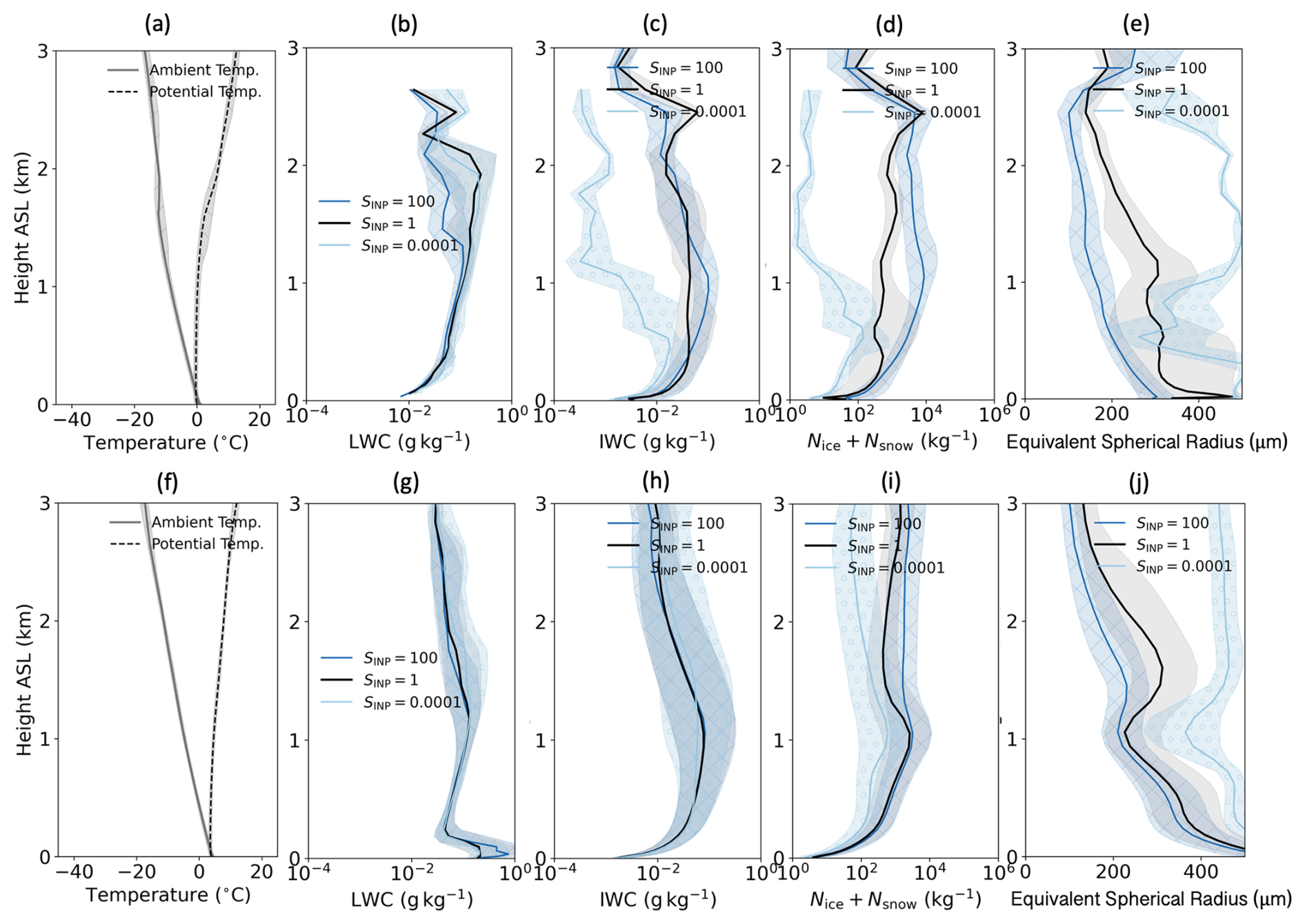
Figure 12 Vertical profiles for in-cloud properties in the October case: ambient temperature (default configuration), potential temperature (default configuration), in-cloud liquid water content (LWC), in-cloud ice water content (IWC), N_ice+N_snow, and equivalent spherical radius for stratocumulus-dominated (a–e) and cumulus-dominated (f–j) regions in the 24 October 2022 CAO case with different S_INP. The solid lines are medians, and the shaded areas are values between the 25 % quantile and 75 % quantile. For the cloud properties plots, grids with less than 10⁻⁶ kg kg⁻¹ total water content are removed. For hydrometeor number concentrations, cloudy grids with less than 1 m⁻³ are removed.

The strengths of the cloud responses to high S_INP and low S_INP are different in the two cases in the stratocumulus-dominated regions. Low S_INP has the strongest effect in March, while high S_INP has the strongest effect in October. This is because the March control simulation has low liquid water (Fig. 11b and c) to be further removed when S_INP increases, while the October control simulation has a very high liquid fraction (Fig. 12b and c), so a high S_INP can strongly convert the liquid to ice with subsequent ice removal through accretion. This is similar when considering the influence of low S_INP for the two cases.

The responses of cloud cover to S_INP perturbations are opposite in these two cases in the cumulus-dominated region: a high S_INP results in higher cloud cover in March but lower cloud cover in October. The response in October is similar to the previous studies and hence not further discussed here. The higher cloud cover in March from a higher S_INP is the result of a slower snow autoconversion and smaller ice hydrometeor size (Fig. 11j) for lower fall speed and hence a lower precipitation rate. As there is very limited liquid in the control simulation already and the dominant precipitation type (the main way to remove cloud water) in March is snow, the impact of having more ice to remove more liquid is very limited in March, and instead we see a similar influence from having more INPs in precipitating mixed-phase clouds to the one from having more CCNs in precipitation liquid-only clouds (the Albrecht effect). Such response is also expected in cirrus clouds with more INPs. This also explains why there is no such influence in the stratocumulus-dominated region, as the precipitation rate is very low.

The influence of S_INP on in-cloud LWP in the March cumulus-dominated region is also suppressed when compared to the one in the stratocumulus-dominated region. This is due to the liquid water being rapidly removed during SCT, as shown in Fig. 6h. We also find that lower S_INP leads to higher LWP but lower albedo at the top of the atmosphere in the March cumulus-dominated region. This is the result of the compensation between a slightly increased LWC (Fig. 11g) near cloud top and a decrease in the albedo of ice through increasing ice size (Fig. 11j) – a Twomey-like effect from INPs.

Most responses of the cloud properties to N_d in both cases and all regions have the same direction (same sign of the fractional changes), but the influence of perturbing N_d on the October CAO clouds is much stronger. This can also be explained by the different liquid–ice partitionings in the control simulations of the two cases, with the October case having a much higher in-cloud LWP.

The strongest influence of perturbing E_HM on cloud proprieties is in the cumulus-dominated region of the October case. There are limited effects of perturbing E_HM in March because the ambient temperature for the March case is too cold and outside of the HM active range (Fig. 11a and f). In the cumulus-dominated region of the October case, both high and low E_HM simulations result in more reflected radiation, but the underlying reasons are different. For the simulation with high E_HM, the higher albedo comes from the higher cloud cover, while for the simulation with low E_HM, it comes from the higher in-cloud LWP.

The responses of cloud properties in the overall domain are determined by not only the responses in the stratocumulus- and cumulus-dominated regions but also the sizes of these two regions and the SCT region. As the selected domains of CAO clouds in both cases have bigger cumulus-dominated regions than the stratocumulus-dominated regions, the overall responses of cloud properties shown here are more similar to the ones in cumulus-dominated regions, with some influences from the stratocumulus-dominated regions.

3.5 Comparison with satellite retrievals

In this section, we explore the extent to which the changes in INP, droplet number, and secondary ice production alter the comparison with multiple satellite-retrieved cloud properties (all-sky LWP, top-of-atmosphere shortwave flux, and top-of-atmosphere longwave flux) in Fig. 13 for March and Fig. 14 for October. The satellite retrieval time and the selected corresponding model output time are concluded in Appendix A. The figures shown in the main text include only the model output with different S_INP; comparison to simulations with N_d and E_HM are shown in Figs. J1 and J2 of Appendix J. Cloud fractions retrieved from MODIS were also used for model–observation comparison, as shown in Figs. J3 and J4. As the cloud fractions from MODIS were calculated by the percentage of cloudy pixels from finer resolution in a 5 km resolution pixel, we created a cloud mask from our model (1.5 km grid spacing) using 20 % cloud cover as a threshold and then derived the cloud fraction using the percentage of cloudy grids in each corresponding MODIS cloud fraction grid.

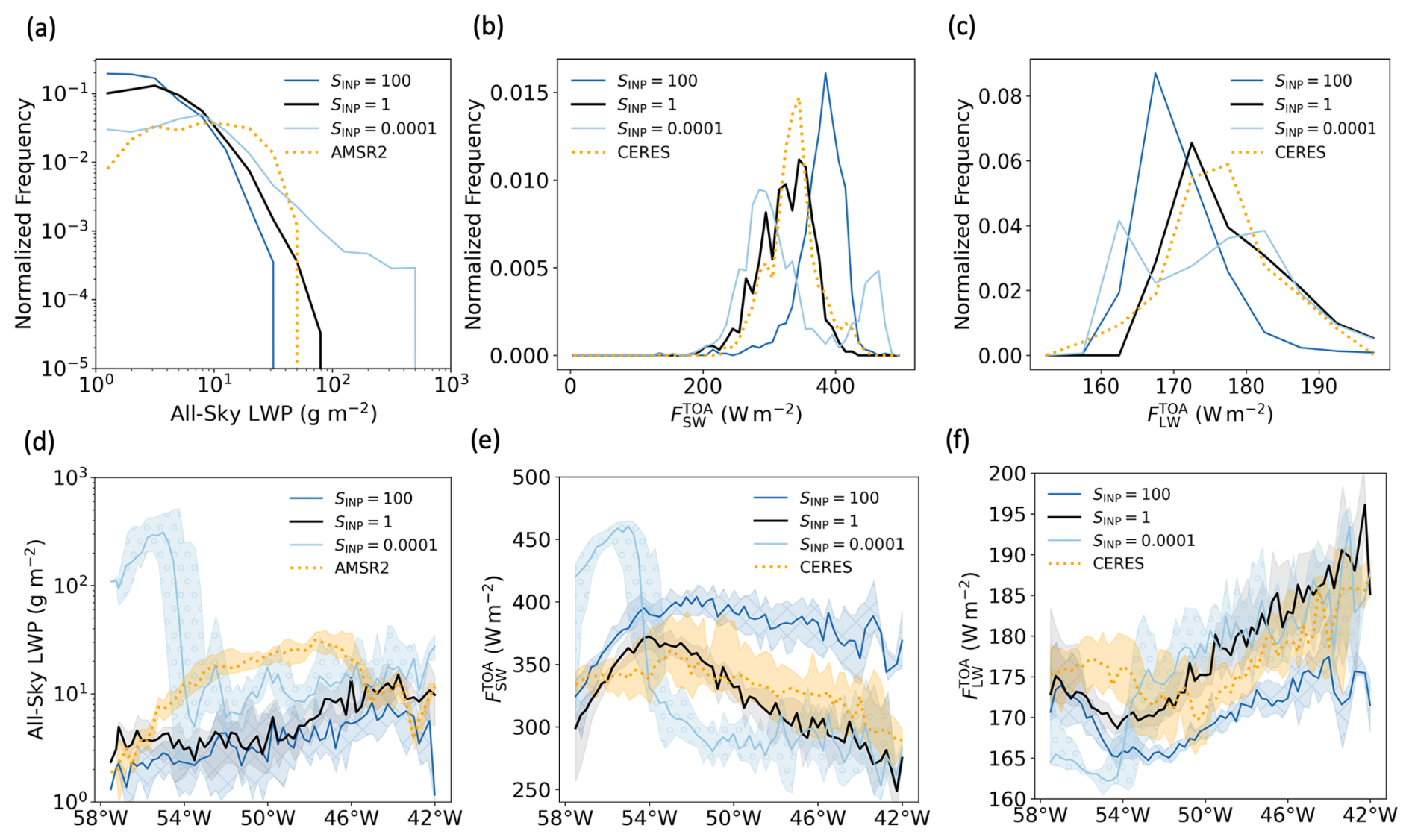
Figure 13 Model output compared with satellite retrievals of the all-sky liquid water path (LWP) from AMSR-2 and shortwave radiation and longwave radiation at the top of the atmosphere from CERES for simulations with different S_INP on 15 March 2022: (a–c) are the normalized frequency, and (d–f) are the cross-section median and quantile comparisons. All the comparisons were done within the selected sub-domain, with the model output and satellite retrievals regridded to the same resolution. The times of model output were selected as the closest quarter to the satellite retrieval times.

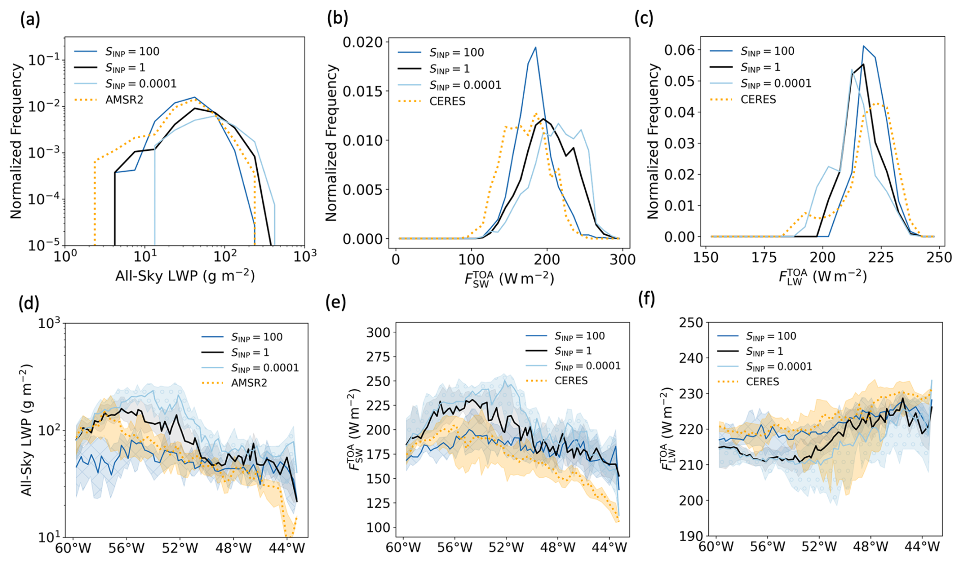
Figure 14 Model output compared with satellite retrievals of the all-sky liquid water path (LWP) from AMSR-2 and shortwave radiation and longwave radiation at the top of the atmosphere from CERES for simulations with different S_INP on 24 October 2022: (a–c) are the normalized frequency, and (d–f) are the cross-section median and quantile comparisons. All the comparisons were done within the selected sub-domain, with the model output and satellite retrievals regridded to the same resolution. The times of model output were selected as the closest quarter to the satellite retrieval times.

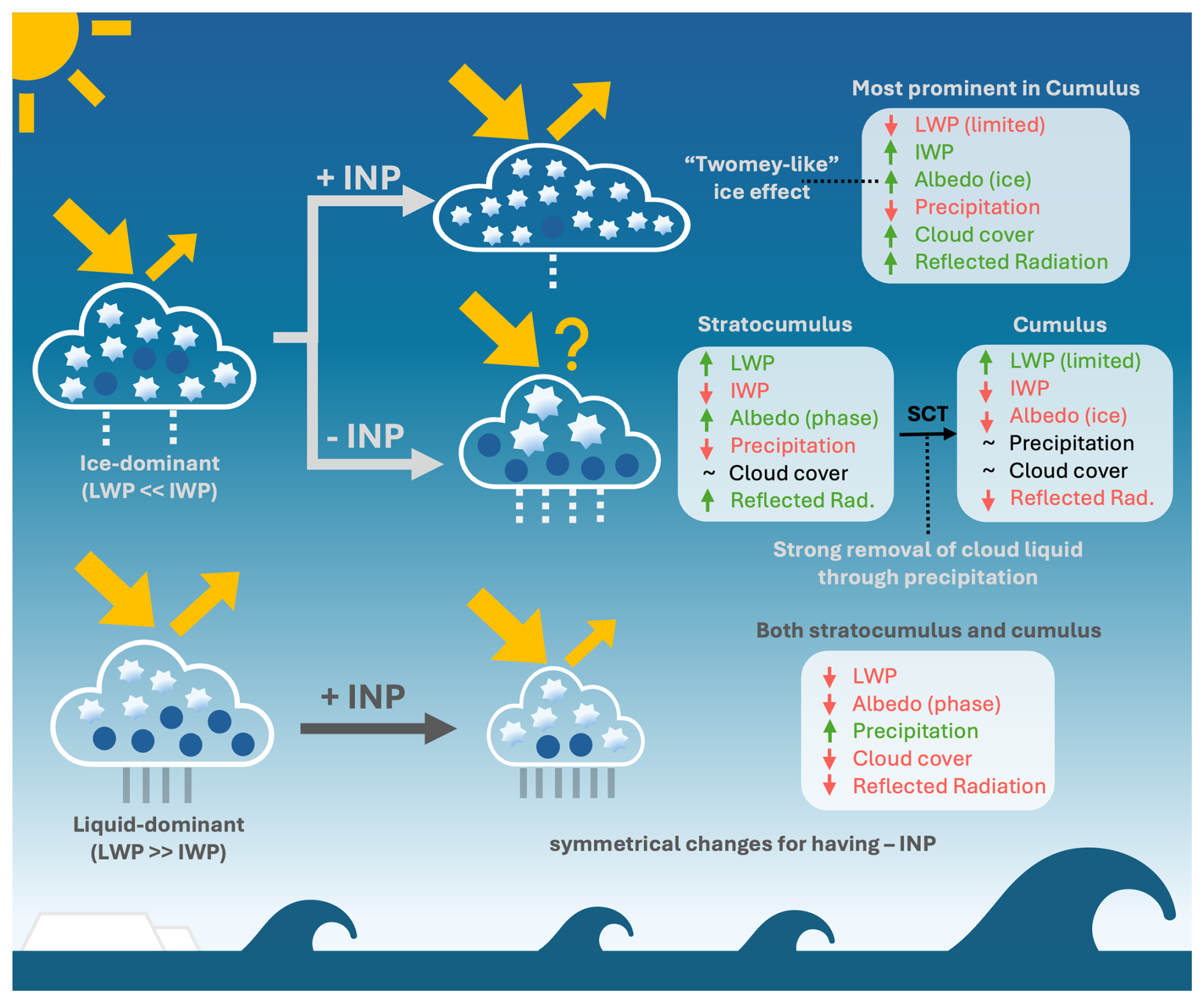
Figure 15 A schematic diagram explaining the different sensitivities of CAO cloud properties to perturbations of INPs in ice-dominant and liquid-dominant clouds.

For all the comparisons, our model output was first regridded to the same spatial resolution as the satellite retrieval, and we focused only on the data within the sub-domain, as shown in Fig. 4a and c, for the model–observation comparison. The normalized frequency and cross-section mean (±1 standard deviation) were used for the comparison. MODIS-retrieved LWP was not used for quantitative comparison here due to its high mixed-phase cloud bias (Khanal and Wang, 2018).

In the March case, the control simulation shows reasonably good agreements of SW and LW fluxes at the top of the atmosphere compared with other sensitivity test simulations, though it underestimates the all-sky LWP from approximately 54 to 46° W (approx. 10 g m⁻² lower for the domain-mean LWP compared to the AMSR-2 retrievals (Fig. 13)). With low S_INP, a higher all-sky LWP is produced but leads to a very large overestimation of all-sky LWP at the beginning of the CAO cloud field. Small underestimation of the SW flux and overestimation of the LW flux are also seen near the eastern boundary of the sub-domain in the control simulation, which may due to the cloud cover and IWP in the control simulation being slightly lower than those observed.

Although our model underestimates the LWP, the LWP from AMSR-2 retrievals suggests that the liquid water was very small in this March case (domain mean around 17 gm⁻²). Clouds in the March case were dominated by ice with a high IWP (modelled domain mean around 632 gm⁻²), and the control simulation shows good agreement of IWC against the CALIOP retrievals (Appendix D). Therefore, we suggest that our model agrees with the observations on the liquid–ice partitioning and that the CAO clouds in this March case were dominated by ice, on which we based our conclusions.

The simulation with a high S_INP in the October case agrees with all satellite retrievals from approximately 56 to 46° W(Fig. 14), but it strongly underestimates the LWP for the region from 60 to 56° W and overestimates the LWP for the eastern end of the region. The simulations with default and low S_INP reproduce the LWP for the region from 60 to 56° W but overestimate the LWP for the rest of the region. Such overestimation of LWP in the cumulus-dominated region for the control simulation may come from the overestimation of LWC and underestimation of IWC in Fig. D5 when model outputs are compared to the M-Phase C323 measurements. Similar biases are seen for the SW flux, which may be the results of LWP bias from the simulations. The overestimation of the SW flux can be reduced by using a low N_d, as shown in Fig. J2 of Appendix J, but such change has limited influence on the all-sky LWP bias. Based on the INP measurements from the M-Phase aircraft campaign, it is known that the measured INP concentrations in this October case are within the range of INP concentrations from default S_INP and low S_INP, but both simulations show clear overestimation of the LWP and SW flux here. This inconsistency may come from the fact that we are only doing a sensitivity test here instead of exploring the whole parameter space, missing the output from different combinations of the parameter values. There are other processes (e.g. mixing and other cloud microphysics processes) that are not investigated in this study; the INP concentrations are temperature-dependent but not directly derived from the background aerosols, and we are potentially missing variations of INPs through CAO cloud development.

4 Discussion and conclusions

In the “Results” section above, we illustrate that the responses of modelled CAO cloud properties to the perturbations of N_d, S_INP, and E_HM are different or even opposite in the two selected CAO cases over the Labrador Sea. Clouds in the October case respond similarly to increases in INP concentration (or ice concentration) compared to previous studies, which is a reduction in reflected SW flux and albedo at the top of the atmosphere (Vergara-Temprado et al., 2018) and an earlier transition from stratocumulus to cumulus clouds (Abel et al., 2017; Tornow et al., 2021). However, the March case differs strongly from the existing literature. We explain this difference in behaviour by categorizing the March case as an ice-dominated regime and the October case as a liquid-dominated regime (Fig. 15).

Cloud temperatures are very different in the March and October CAO cases, with the mixed-phase CAO clouds in March being in a much colder environment (approximately 15–20 °C lower). Such temperature difference leads to a strong difference in primary ice production through INP, as the INP concentration increases exponentially with decreasing temperature using the same parameterization (approximately 2 orders of magnitude for the 20 °C difference). A higher primary ice production (colder cloud temperatures) means that a greater portion of the condensed cloud water is converted to ice, resulting in a lower liquid water fraction in March, and vice versa for lower primary ice production (warmer cloud temperatures) in October.

The March CAO event is in an ice-dominated regime with a low liquid water fraction. In such an ice-dominated regime, increasing the INP concentration leads to a higher number concentration of ice (N_ice), slows down the snow autoconversion rate, and reduces the ice hydrometeor size and fall speed, which then reduces the precipitation and restricts the removal of cloud water. This is more obvious in the cumulus-dominated region, as it experiences stronger precipitation than the stratocumulus-dominated region. Such influence leads to higher cloud cover and IWP in March and consequently a higher TOA albedo and SW flux, which is further enhanced by the higher single-scattering albedo from the high N_ice (Twomey-like effect). These behaviours are similar to the aerosol first (Twomey, 1977) and second (Albrecht, 1989) indirect effects on liquid clouds through changes in cloud condensation nuclei concentrations but, in this March case, acting through INP concentrations. As the clouds are dominated by ice, there is also very little water available for liquid-phase processes; therefore, changes in N_d have only a small influence on the clouds. Furthermore, because the cloud temperatures are low (approx. −15 to −35 °C for cloudy grids) and the Hallett–Mossop process is assumed to occur only in the temperature range from −2.5 to −7.5 °C, changing E_HM has only a small influence on the clouds.

The response of TOA albedo to increased S_INP simulation in March identifies a possible new mechanism of negative cloud-phase feedback if INP concentrations increase in the future, in addition to the original three mechanisms suggested in Murray et al. (2021). For ice-dominated clouds with increasing INP concentrations from the warming climate, it will respond to the higher INP concentration in similar radiative responses to that seen in liquid clouds when CCNs increase (i.e. an INP-driven first and second indirect effect), leading to a higher SW flux at the top of the atmosphere and negative cloud-phase feedback, competing with the effect of warming these cloud systems.

With low INP concentrations in the March CAO event, different responses are seen in the stratocumulus-dominated and cumulus-dominated regions. In the stratocumulus-dominated region, a higher in-cloud LWP and lower surface precipitation with no obvious change in cloud cover result in increased reflected radiation. In the cumulus-dominated region, as the cloud liquid is rapidly removed during SCT, the increase in in-cloud LWP from low INP concentration is therefore very limited. Instead, lower IWP and lower ice albedo from the Twomey-like effect result in less SW reflection, compensating the limited increase in LWP.

Contrary to the March case, the warmer October case is in a liquid-dominated regime with a high liquid water fraction in general (apart from the end of the CAO cloud system). In this liquid-dominated regime, increases in INP concentration lead to higher N_ice and therefore a higher collection of liquid water from ice hydrometeors and consequently more precipitation, stronger removal of cloud water, and lower cloud cover, opposite to the March case. Together with lower LWP, increasing the INP concentration in such a liquid-dominated regime leads to a lower SW flux at the top of the atmosphere. As the liquid water fraction is high, there is also a strong influence from changing N_d and consequently a larger effect on the SW flux from changes in liquid water than in March. Because the temperatures are relatively high, more clouds are in the active temperature range for the HM process, and there is enough liquid water available for riming; hence, we see a strong influence from changing E_HM.

The occurrence of liquid- and ice-dominated clouds, which controls their response to INP, N_d, and E_HM, is controlled not only by temperature but also by the ambient INP concentration: for example, the cloud is liquid-dominated at the beginning of the March CAO cloud system in the low S_INP simulation. This suggests that there could be an interaction between INP concentrations and other cloud properties, such as a strong effect of N_d on cloud properties at very low INP concentrations but a weak dependence at high INP concentrations when the cloud is ice-dominated. This illustrates one of the limitations of this study, as we have explored the effects of only individual parameters. A full PPE (perturbed parameter ensemble) that explores potential co-variations in inputs and interactive effects would be needed to explore this further. In addition, we compared only two cases and their environmental conditions in this study; a more robust and systematic investigation of the influence of environmental conditions can also be carried out using a PPE in which environmental/initial conditions are varied using idealized simulations.

Other secondary ice production (SIP) mechanisms were not included in our model when this work was conducted, although the non-included SIP mechanisms (such as droplet shattering and ice–ice collision) have been shown to be important to SCT in CAO events (Karalis et al., 2022). These two SIP mechanisms can take place at a colder temperature than the existing HM process, which could have some impacts on the CAO cloud properties and responses in the cold March case (e.g. higher ice number concentrations and smaller ice hydrometeor sizes). Future modelling work will include other SIP mechanisms when these become available in the model. In addition, fixed in-cloud N_d was used in this study for easier interpretation of the sensitivity test results, but such a setup can lead to potential feedbacks between cloud and aerosols/CCNs being neglected. Future work will also include aerosol-derived N_d and cloud processing of aerosols where possible for a better representation of aerosol–cloud interactions.

In general, this comparative sensitivity study reveals different or even opposite responses of the CAO cloud properties to aerosols, including CCNs (through changing N_d) and INPs and SIP (the Hallett–Mossop process), when the cloud temperatures are different by comparing two CAO events over the Labrador Sea. The main findings and conclusions drawn from this study are shown below.

1. Cloud temperature and INP concentrations control the liquid–ice partitioning in the control simulations and thereby affect their responses to the perturbed parameters. The two cases have different liquid–ice partitioning and hence are categorized into ice-dominated (the cold March case) and liquid-dominated (the warm October case) regimes.

2. In the liquid-dominated, warm October case, increasing INP concentration leads to lower cloud cover and in-cloud LWP, hence a lower albedo, consistent with findings from previous studies.

3. In the ice-dominated, cold March case, increasing INP concentration leads to higher cloud cover and in-cloud IWP, hence resulting in a higher albedo and SW flux at the top of the atmosphere. Such response is more prominent in the cumulus clouds. This influence of increasing INP concentration is opposite to the one in the liquid-dominated October case and is potentially a new mechanism of negative cloud-phase feedback in ice-dominated CAO clouds if INP concentrations increase in the future due to the warming climate, in addition to the original three cloud-phase feedback mechanisms suggested by Murray et al. (2021).

4. Stronger influences from changing N_d and the Hallett–Mossop efficiency are seen in the liquid-dominated October case, as more liquid is available and the cloud temperature in October spans the HM active temperature range (−2.5 to −7.5 °C).

Future work with a full exploration of the parameter space (including other SIP mechanisms), systematically perturbed environmental conditions, or other important cloud microphysics parameters will be beneficial to our understanding and modelling of these mixed-phase CAO clouds and their responses to the warming climate.

Appendix A: Retrieval time and selected model time point for satellite data used in this study

Table A1 The satellite products used in this study, their retrieval times, and the selected model time points for comparison in the sub-domains. LWP: liquid water path, SW: shortwave, LW: longwave, CTT: cloud top temperature, CWP: cloud water path, IWC: ice water content, n/a: not applicable.

Appendix B: Monthly distribution of cloud top temperature over the Labrador Sea in 2022

The monthly distribution of cloud top temperature of low-level (cloud top pressure >700 hPa) and mixed-phase (cloud top temperature ranging from −40 to 0 °C) CAO cloud over the Labrador Sea in 2022 is shown here in Fig. B1.

The daily-mean CAO index at 800 hPa (M₈₀₀) (Kolstad and Bracegirdle, 2008; Fletcher et al., 2016a), which is the difference between the potential temperature at the surface skin (θ_skin) and the potential temperature at 800 hPa (θ₈₀₀), i.e. $M_{\mathrm{800}}={\mathit{\theta }}_{\text{skin}}-{\mathit{\theta }}_{\mathrm{800}}$, was calculated using the ERA5 dataset (Hersbach et al., 2020). Grids with M₈₀₀>0 K, which is a compulsory condition for CAO identification and an indicator of an unstable atmosphere, were defined as CAO grids. We use θ₈₀₀ in this study because more high-latitude CAOs can be identified by using θ₈₀₀ compared with using θ₇₀₀ (potential temperature at 700 hPa) (Fletcher et al., 2016a). Cloud top pressure (CTP) and cloud top temperature (CTT) from MODIS were used to filter low-level (CTP >700 hPa), mixed-phase (−40 °C < CTP <0 °C) clouds.

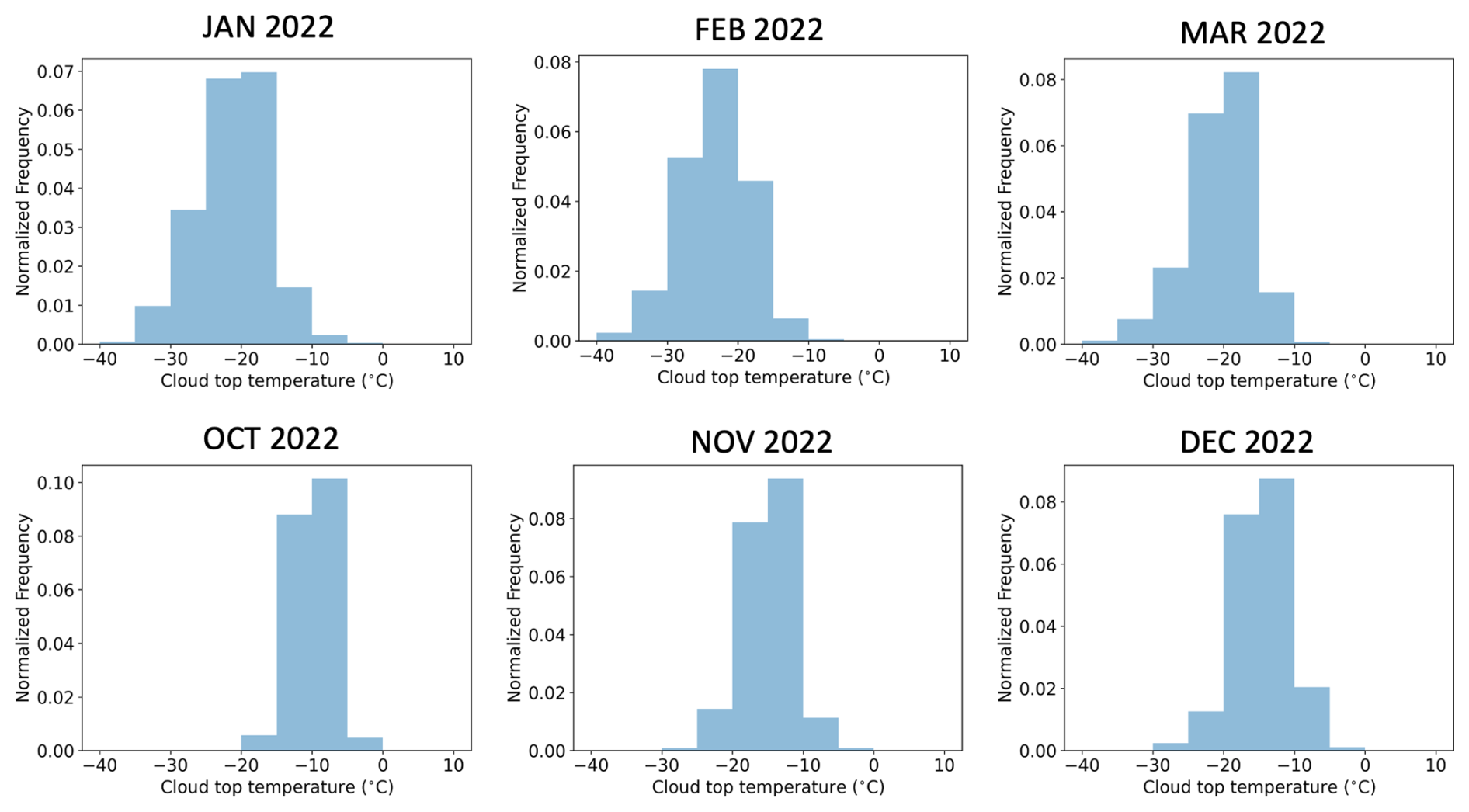
Figure B1 Monthly distribution for cloud top temperature of low-level, mixed-phase CAO clouds over the Labrador Sea in January, February, March, October, November, and December 2022. Clouds with cloud top pressure lower than 700 hPa and cloud top temperature higher than 0 °C and lower than −40 °C were excluded.

CTTs of low-level, mixed-phase CAO clouds in January, February, and March are generally lower, with CTT peaks between −20 and −25 °C, while the ones in October, November, and December are higher, with CTT peaks between −10 and −15 °C. Other months were not included due to the low density of CAO events in those time of the year. The cold March case in this study is located near the colder end of the CTT climatology, whereas the warm October case is located near the warmer end, providing contrasting CTT conditions for this sensitivity test and a study range covering most of the range from the shown CTT climatology.

Appendix C: Maps for the nested model domains and the sub-domains for analysis

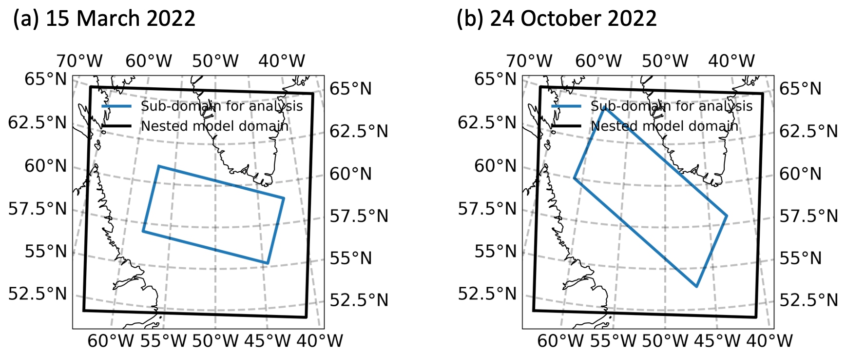
Figure C1 Nested model domains (black) and the selected sub-domains for analysis (blue) for (a) 15 March 2022 and (b) 24 October 2022.

Figure C1 shows the nested model domains and the sub-domains for analysis of both cases. The sub-domains were chosen to be away from the boundaries of the nested model domains to avoid boundary effects. In both cases, due to the winds and air masses from the northwest direction, the fields generated from the coarser global model required a few hours to spin-up once entering the nested model domains.

The timescale for spinning up the boundary layer structure in the nested model domain is $\frac{L}{{\mathit{\sigma }}_w}$, where L is the boundary layer depth ( 1000 m at the beginning of the CAO events) and σ_w is the standard deviation of the w component of wind. For the March case, the mean σ_w between the western boundaries of the nested model domain and the sub-domain is around 0.83 ms⁻¹, which requires about 20 min to spin up. For the October case, the mean σ_w between the northwestern ends of the nested model domain and the sub-domain is around 0.39 ms⁻¹, which requires about 45 min to spin up.

We examined whether the boundary effects can reach the sub-domains by using simple calculations of how long it takes the air masses to reach the western boundary of each sub-domain. The distances were estimated based on the mean direction of the wind. For the March case, the distance from the middle of the western boundary of the nested model domain to the middle of the western boundary of the sub-domain is around 430 km. The mean wind speed from the surface to 2 km in height above sea level (a.s.l.) is 13.0 ms⁻¹ (46.8 km h⁻¹). Therefore, it takes around 9 h for the air masses to travel in the March case. For the October case, the distance from the northwest point of the nested model domain to the middle of the western boundary of the sub-domain is around 500 km. The mean wind speed from the surface to 2 km in height a.s.l. is 16.5 ms⁻¹ (59.4 km h⁻¹). Thus, it takes around 8.5 h for the air masses to travel in the October case. Some air masses travelling into the northwestern part of the sub-domain may have less time to spin up and may be affected by the boundary effects; however, we chose to keep this part of the sub-domain in order to capture more earlier-stage CAO clouds, as the clouds broke up into cumulus clouds very early on in the October case.

For the whole sub-domain in the March case and most of the sub-domain (except the small northwestern part) in the October case, the time and distance required for the air masses to reach the sub-domains are sufficient to avoid boundary effects propagating into the sub-domain.

Appendix D: Model–observation comparison for control simulations

In this Appendix, we validate our control simulations using satellite retrievals for the March case (as there is no aircraft campaign for this case), as shown in Figs. D1, D2, and D3, and using M-Phase aircraft measurements for the October case, as shown in Fig. D5 from two flights (M-Phase C322 and C323), with the flight tracks shown in Fig. D4. The results of the model–observation comparison for the March case are shown first, followed by the results for the October case.

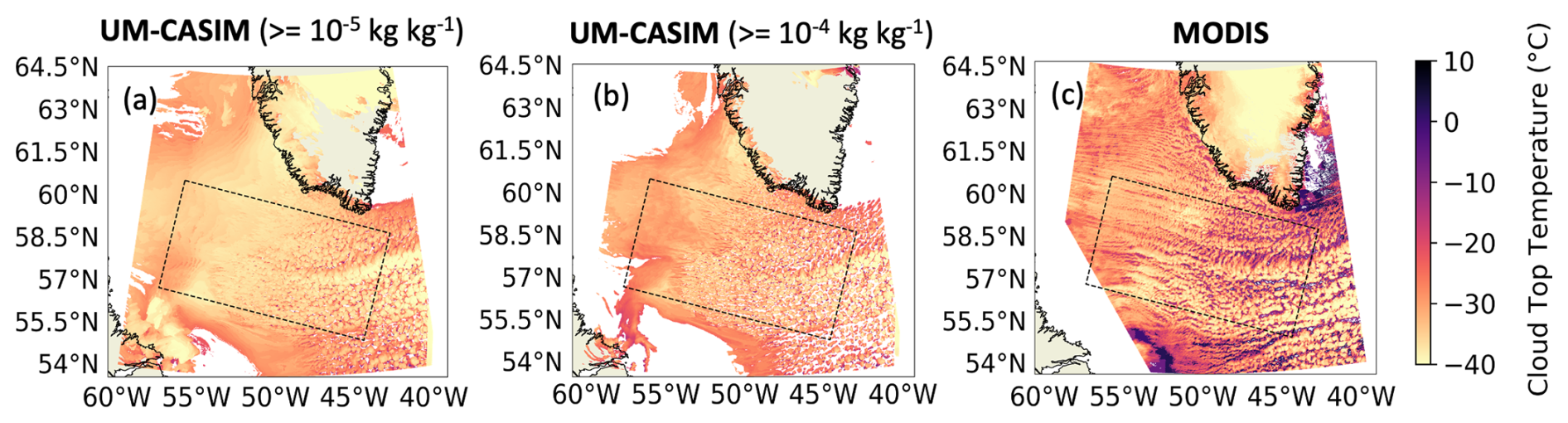
Figure D1 Cloud top temperature (CTT, a–c) from the control simulation of the March case and the MODIS on board the Aqua satellite. Two TWC (total water content) thresholds were used to determine whether a model grid is cloudy or not: TWC $\ge {\mathrm{10}}^{-\mathrm{5}}$ kg kg⁻¹ (a) and TWC $\ge {\mathrm{10}}^{-\mathrm{4}}$ kg kg⁻¹ (b). Regions marked with grey dashed lines in (a)–(c) are the sub-domains (the same as the sub-domains shown in the main content) for the comparison of CTT distributions in Fig. D2.

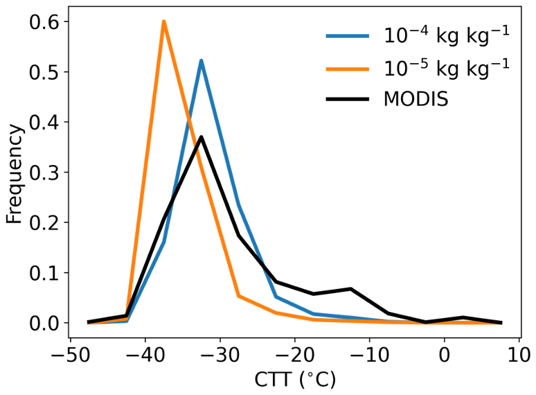
Figure D2 Comparison of the cloud top temperature (CTT) distributions of 15 March 2022 between the CTT retrieved from the MODIS on board the Aqua satellite (black) and the CTT extracted from the control simulation of the March case using different total water content thresholds: TWC $\ge {\mathrm{10}}^{-\mathrm{5}}$ kg kg⁻¹ (orange) and TWC $\ge {\mathrm{10}}^{-\mathrm{4}}$ kg kg⁻¹ (blue).

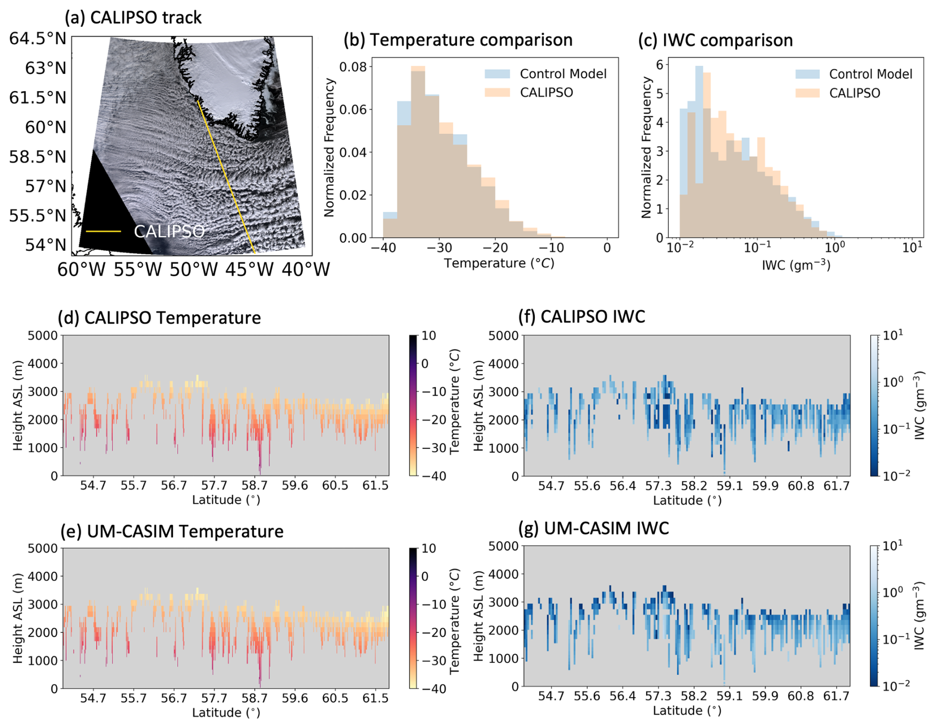
Figure D3 Comparison of temperature and IWC (ice water content) profiles from CALIOP on board the CALIPSO satellite and the control simulation of 15 March 2022: (a) the selected CALIPSO track, (b) distributions of temperature, (c) distributions of IWC, and (d) regridded CALIPSO temperature profile. (f) CALIPSO IWC profile, (e) modelled temperature profile, and (g) regridded modelled IWC profile. Note that for the comparison and individual profiles, grids without valid CALIOP data or model data are removed.

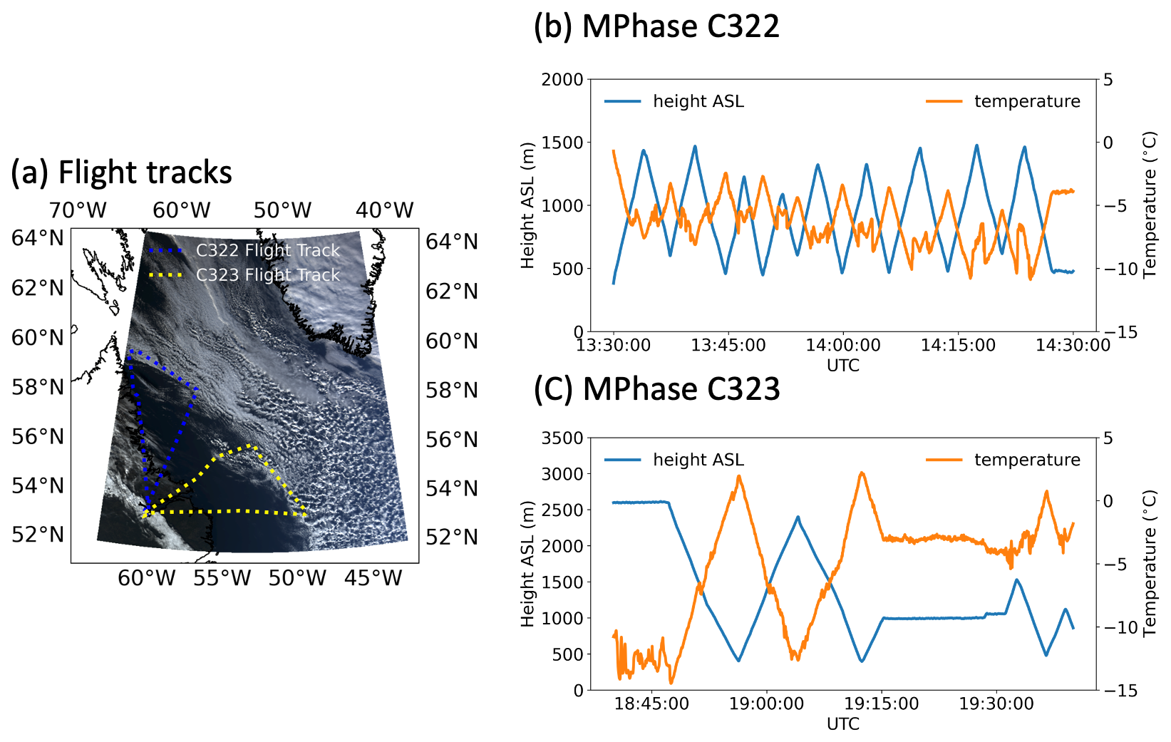
Figure D4 Information of the M-Phase C322 and C323 flights used for the validation of the control simulation on 24 October 2022: (a) flight tracks, (b) height and temperature profiles for cloud measurements during M-Phase C322, and (c) height and temperature profiles for cloud measurements during M-Phase C323.

D1 15 March 2022

For the March case studied in this work, we evaluate our model against cloud top temperature (CTT) from MODIS on board the Aqua satellite, as well as temperature and ice water content (IWC) from CALIOP on board the CALIPSO satellite (Level-2 1 km Cloud Layer Data for temperature and Level-2 5 km Cloud Layer Data for IWC, version 4-51).

Figure D1 shows the CTT from the model output and MODIS retrievals. As a satellite simulator was not available for regional simulations in our model, the extraction of modelled CTT relied on the definition of cloudy grids. Here, we used two thresholds of grid-box mean TWC (total water content) for determining whether a grid in our model output is cloudy or non-cloudy. The threshold 10⁻⁵ kg kg⁻¹ has been used before for comparing model water content with in situ aircraft measurements (e.g. Abel et al., 2017), and the threshold 10⁻⁴ kg kg⁻¹ was selected for a stricter definition of cloudy grids, as passive satellite retrievals can be less sensitive compared to aircraft measurements. As there are no high clouds in the domain of interest, the cloud top for each column of model grids was defined as the highest grid passing the selected threshold of TWC. The MODIS data (1 km) were regridded to the model resolution (1.5 km) using the nearest-neighbour method.

The cloud top height (CTH) retrieved from MODIS is around 5 km for low-level clouds (not shown), which is unreasonable and therefore not further used for validating CTH in the control simulation. This may have occurred because the MODIS CTH above sea level is not directly retrieved but calculated using observed SST (sea surface temperature), CTT, and a zonal mean lapse rate (Platnick et al., 2016), but the CTT in the March case is much lower compared to the climatology.

The distributions of CTTs within the sub-domain shown in Fig. C1a, b, and c are compared in Fig. D2. Using a threshold of 10⁻⁵ kg kg⁻¹ resulted in a much lower CTT (peak near −40 °C) compared to the MODIS-retrieved CTT (peak near −30 °C). Using a threshold of 10⁻⁴ kg kg⁻¹ reduces the cold bias strongly and leads to a similar peak temperature of CTT (near −30 °C) to the one from MODIS. However, a small cold bias still exists, with the modelled CTT using the 10⁻⁴ kg kg⁻¹ threshold having higher frequency at colder temperatures and lower frequency at warmer temperatures compared to the satellite-retrieved CTT. Note that the grid-to-grid bias was not calculated here due to a potential double-penalty problem when comparing model data with observations.

The temperature and IWC profiles from CALIOP on board CALIPSO were also used to evaluate the control simulation of the March case. Figure D3 shows the selected CALIPSO track (a), the comparison of the temperature and IWC distributions (b, c), and the along-track profiles (d–g). The modelled profile was extracted by finding the closest model grid for each footprint from the CALIPSO data. The CALIPSO temperature has a higher resolution (1 km) and therefore was regridded to the model resolution (1.5 km), while the modelled IWC has a higher resolution compared to the CALIPSO IWC resolution (5 km) and therefore was regridded to the CALIPSO IWC resolution. Due to the nature of lidar attenuation for clouds at lower levels, grids that had no CALIPSO data or model data were excluded when comparing the distributions and plotting the profiles.

There is also a small cold bias for the temperature, but the overall temperature distribution from our model agrees well with the one from CALIPSO. This is also shown for the whole profile statistics: the median temperature from the modelled profile is −30.9 °C (interquartile range (IQR): −34.3 to −25.8 °C), and the median temperature from the CALIPSO profile is −30.2 °C (IQR: −33.7 to −25.1 °C).

The distributions of IWC from the model and CALIPSO have similar peak IWC values. However, the modelled IWC has higher frequencies both at the low (0.01–0.02 g m⁻³) and high (0.5–1 g m⁻³) ends of the IWC bins and lower frequencies for the IWC bins in the middle. Based on the profile statistics, the model slightly overestimates the IWC (median: 0.19 g m⁻³, IQR: 0.08–0.39 g m⁻³) compared to the CALIPSO IWC (median: 0.17 g m⁻³, IQR: 0.08–0.33 g m⁻³). However, such bias (0.02 g m⁻³) is considered low and acceptable.

To summarize the model–observation comparison above for the March case, our modelled CTTs are slightly lower compared to the MODIS-retrieved CTTs when using the 10⁻⁴ kg kg⁻¹ threshold. Similarly, the temperature comparison between the modelled profile and CALIPSO profile shows that our model has a small cold bias of the temperature (−0.7 °C), but such bias is acceptable and suggests that temperatures from our model are reasonably comparable with the satellite retrievals. Our model overestimates the IWC by 0.02 g m⁻³ compared to the CALIPSO IWC, but such bias is also relatively small and acceptable, suggesting that the control simulation can also reproduce the IWC reasonably well.

D2 24 October 2022

For the October case, we evaluate the control simulations by comparing the temperature, grid-box mean TWC (total water content), liquid water fraction (LWC/TWC), grid-box mean LWC (liquid water content), and grid-box mean IWC (ice water content) with the aircraft measurements from two flights (C322 and C323) during the M-Phase aircraft campaign. The flight tracks and time-series plots of temperature and height for each flight are shown in Fig. D4. The results of the comparison for the variables mentioned above are shown in Fig. D5. The water content measurements came from Nevzorov probes on board the aircraft.

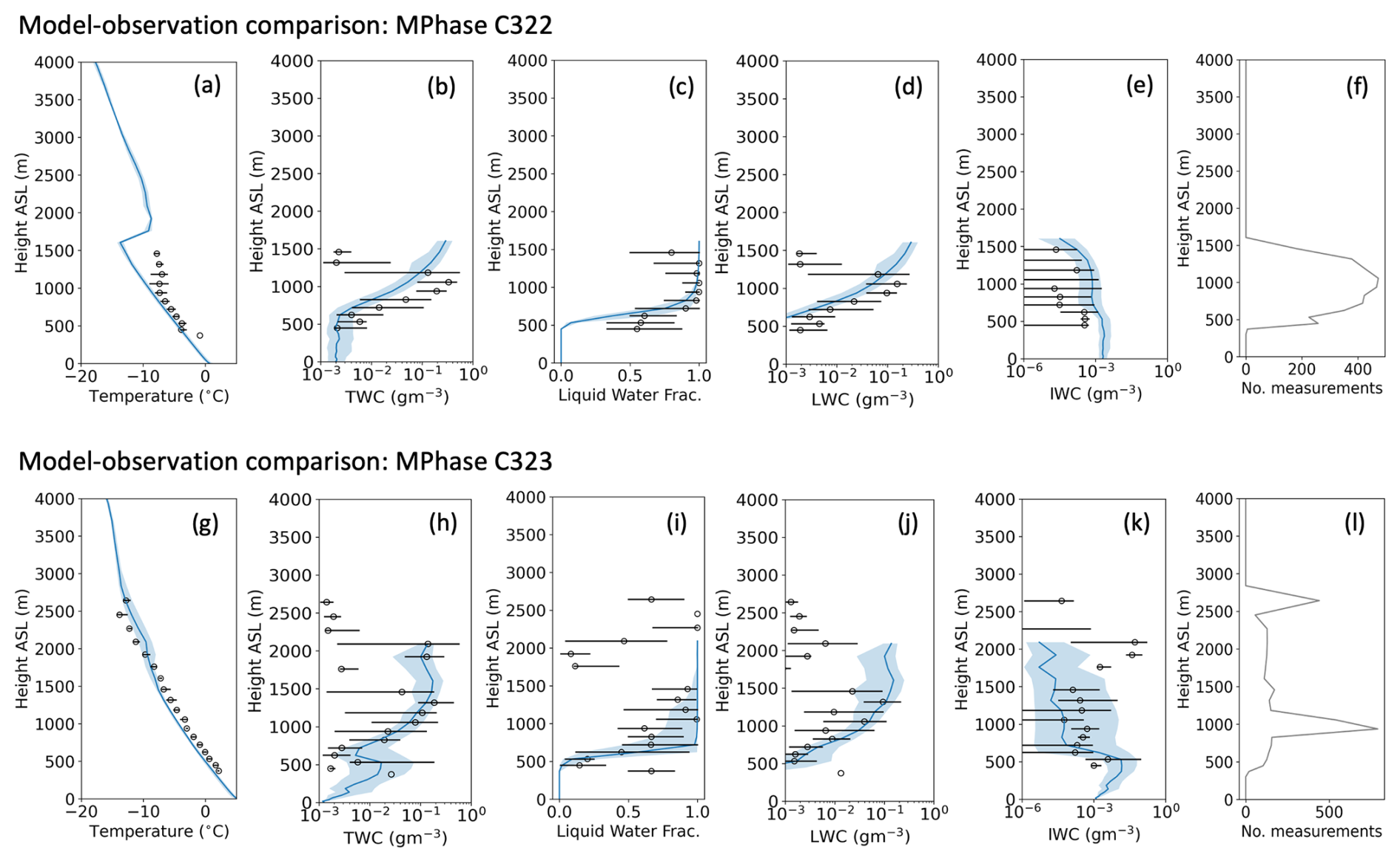
Figure D5 Model–observation comparison of the control simulation against M-Phase C322 and C323 measurements on 24 October 2022: (a, g) temperature, (b, h) grid-box mean TWC (total water content), (c–i) liquid water fraction (LWC/TWC), (d–j) grid-box mean LWC (liquid water content), and (e–k) grid-box mean IWC (ice water content). (f) and (l) show the number of measurements from each flight. Model data are shown as blue lines (medians), with the IQRs (interquartile ranges) coloured in light blue. Observation data are shown as black unfilled circles (medians), with the IQRs shown as black solid lines.

Preprocessing of the aircraft data (1 Hz resolution) and the model data was performed for a like-for-like comparison. Each point of the observation data was assigned to the nearest model grid (longitude, latitude, and altitude), and the mean of all the observed data points within each model grid was calculated for the later comparison with the model data. The model data were extracted using the flight track with grids within 10.5 km around each point of the flight tracks also included. Considering that the model may not simulate the same cloud at the same location as in the real world and that the aircraft measurements may not be representative enough for comparison with the grid-box mean value from the model, we did not calculate the grid-by-grid bias directly but compared the measured variables to the modelled variables using the composited vertical profile of each flight.

For the model–observation comparison with measurements from M-Phase C322, where the dominant type of clouds is stratocumulus clouds, our modelled temperature is lower than the observed temperature above 1000 m (Fig. D5a) and has a higher inversion layer. This may be the reason why the locations of the clouds from our control simulation are higher than the observed clouds (Fig. D5b. Before the calculation of bias, we shifted the modelled clouds lower to match the peaks of the observed cloud profile and modelled cloud profile. The control simulation slightly overestimates the TWC, LWC, and IWC, with profile mean biases of 0.048, 0.047, and 0.0003 g m⁻³, respectively, but is consistent with the observation of the liquid water fraction that most of the clouds were dominated by liquid. Some ice-free conditions were not simulated in our model (Fig. D5e), but such bias needs further model–observation comparison with more cases to investigate, which is beyond the scope of this work.

For the model–observation comparison with measurements from M-Phase C323, where the dominant type of clouds was cumulus clouds, our model shows good agreement of the temperature profile with the observed one (Fig. D5g). Our model did not simulate some high clouds (around 2500 m); however, these clouds were very thin, with the majority of their TWC around 0.001 g m⁻³ (Fig. D5i). Our model reproduced the grid-box mean TWC with a profile mean bias of 0.004 g m⁻³. The LWC was overestimated, with a bias of 0.018 g m⁻³, while the IWC was underestimated, with a bias of −0.003 g m⁻³, resulting in higher liquid water fraction in our model. For clouds ranging from 1500 to 2000 m, our model captured the TWC but with too much liquid and too little ice, resulting in a much higher liquid water fraction. The overestimation of the LWC and liquid water fraction here may be the reason for the overestimation of the all-sky LWP shown in Fig. 14 in the October case.

To summarize the model–observation comparison of the October case, in the C322 region, where stratocumulus clouds dominated, the heights of our modelled clouds were higher for around 500 m, potentially due to the cold bias of the temperature above 1000 m and a higher modelled inversion layer. The grid-box mean TWC, LWC, and liquid water fraction generally agreed with the observation if the modelled clouds were shifted to the same heights as the observed clouds. The modelled IWC biased high compared to the observed IWC but remained as a very small part of the cloud water, similar to the observation. In the C323 region, where cumulus clouds dominated, our model captured the temperature profile but missed some thin (TWC around 0.001 g m⁻³), high (around 2500 m) clouds. For clouds ranging from 1500 to 2000 m, our model overestimated the LWC and underestimated the IWC; this was also seen for clouds below 1500 m but with much smaller bias, which can lead to the overestimation of the all-sky LWP shown in Fig. 14 in the October case.

Appendix E: Supplementary figures for Fig. 5

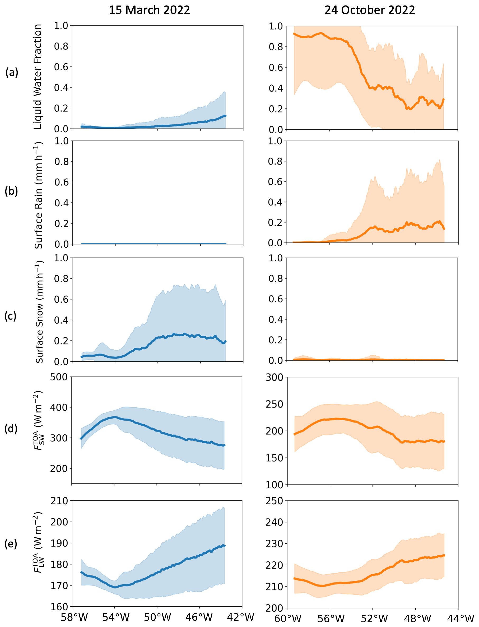
Figure E1 Cross-section mean cloud properties from the March (left panel) and October (right panel) control simulations in the sub-domain: (a) liquid water fraction (LWP/CWP), (b) surface rain rate, (c) surface snow rate, (d) shortwave (SW) radiation flux at the top of the atmosphere, and (e) longwave radiation (SW) flux at the top of the atmosphere. The shaded area indicates the range of ±1 standard deviation. The time points selected are 16:45 UTC for the March case and 17:00 UTC for the October case, which are consistent with the corresponding CERES measurement times.

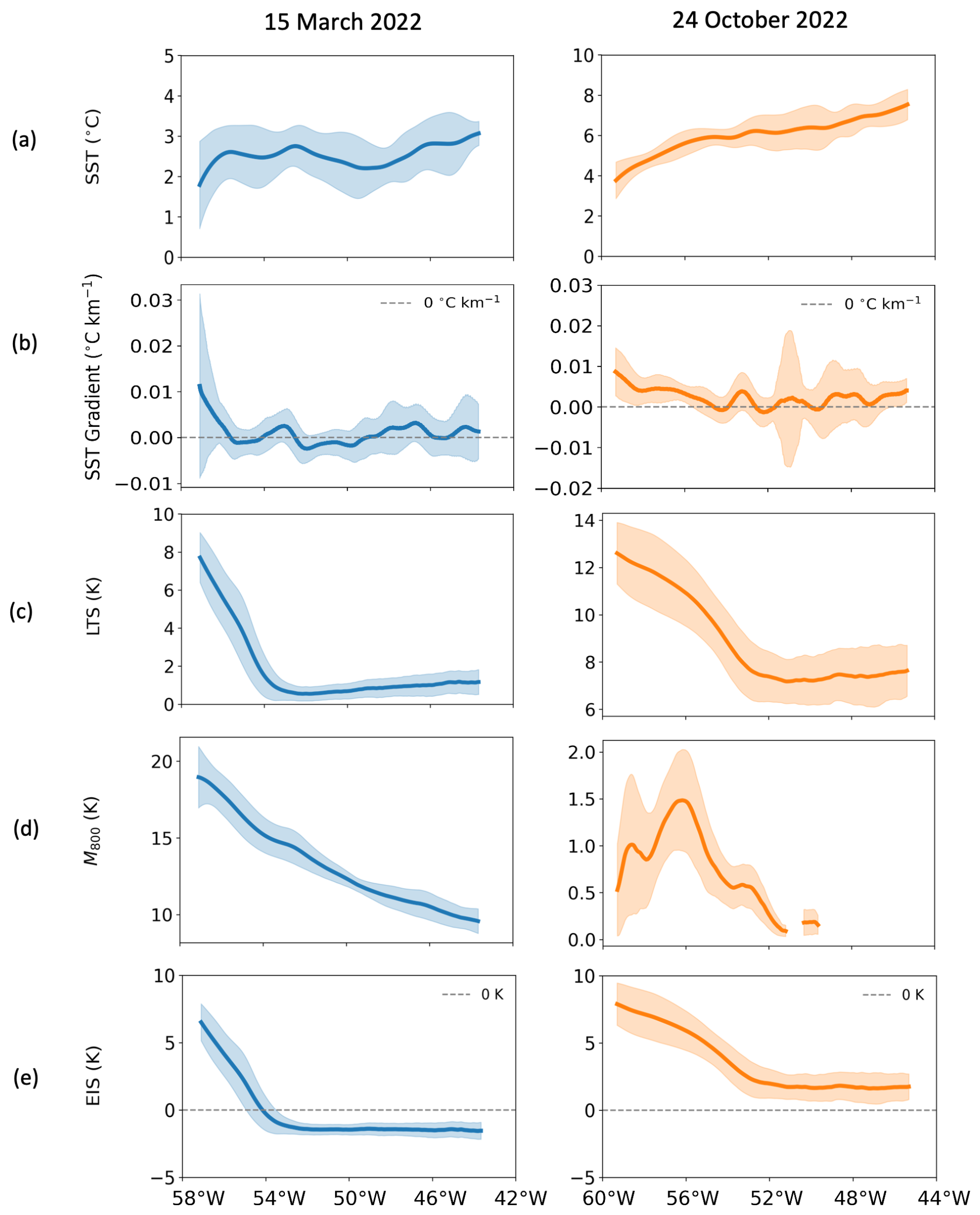
Figure E2 Cross-section mean cloud properties from the March (left panel) and October (right panel) control simulations in the sub-domain: (a) sea surface temperature (SST), (b) SST gradient, (c) lower tropospheric stability (LTS), (d) CAO index at 800 hPa (M₈₀₀), and (e) estimated inversion layer strength (EIS). The shaded area indicates the range of ±1 standard deviation. The time points selected are 16:45 UTC for the March case and 17:00 UTC for the October case, which are consistent with the corresponding CERES measurement times.

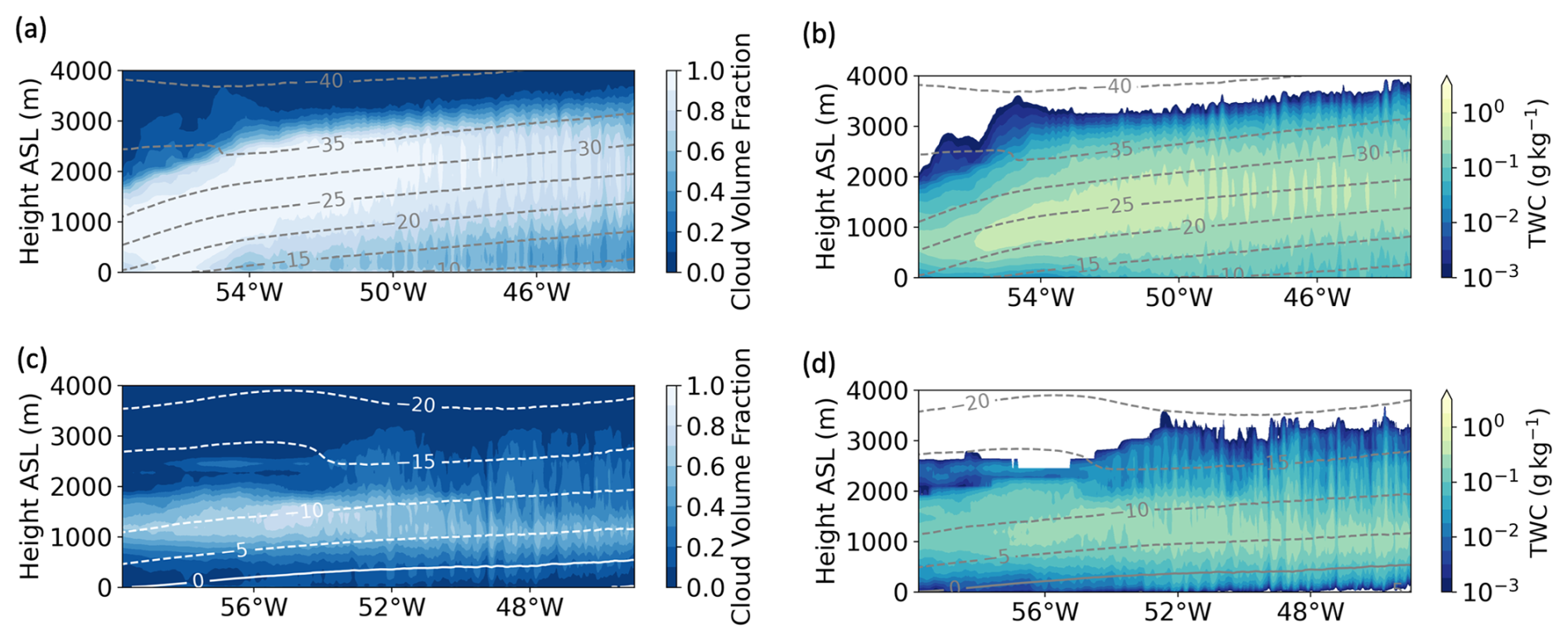
Figure E3 Cross-section mean vertical profiles from the sub-domain of bulk cloud volume fraction and in-cloud total water content (TWC) for the March case (a, b) and the October case (c, d) in the control simulations. Dashed lines in all figures are the ambient temperature contour lines in °C. To calculate the mean of the in-cloud total TWC, grid boxes with cloud volume fractions lower than 5 % and total in-cloud TWC less than 1 g kg⁻¹ are excluded. The time points selected are 16:45 UTC for the March case and 17:00 UTC for the October case, which are consistent with the corresponding CERES measurement times.

Appendix F: Supplementary figures for Figs. 6 and 7

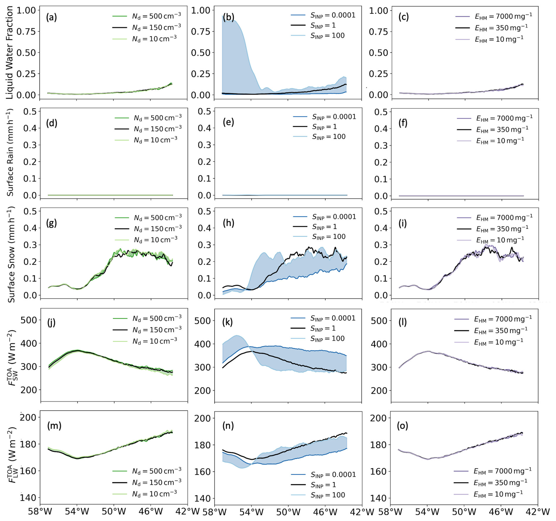
Figure F1 Sub-domain mean CAO cloud properties from the beginning of the cloud system to the end of the cloud system for 15 March 2022 at 16:45 UTC: (a–c) liquid water fraction (LWP/CWP), (d–f) surface rain, (g–i) surface snow, (j–l) shortwave radiation flux at the top of the atmosphere, and (m–o) longwave radiation flux at the top of the atmosphere. Grid boxes with cloud cover less than 20 % were removed before averaging. The time of 16:45 UTC was chosen for the relative CERES (on board the Aqua satellite) measurement time.

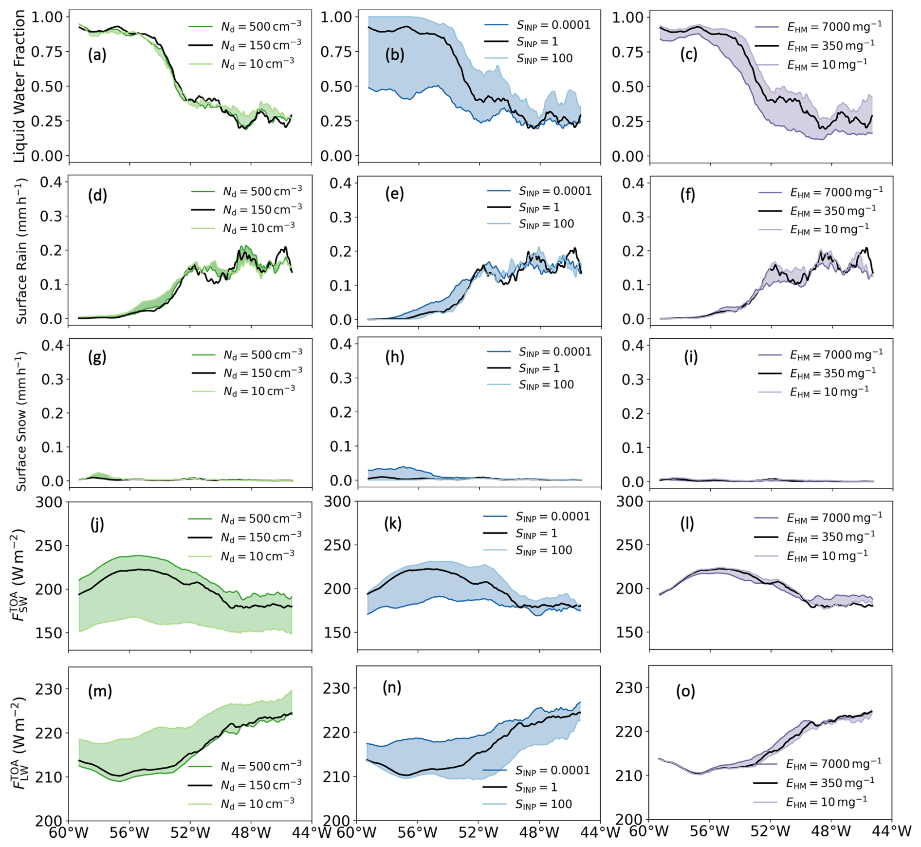
Figure F2 Sub-domain mean CAO cloud properties from the beginning of the cloud system to the end of the cloud system for 24 October 2022 at 17:00 UTC: (a–c) liquid water fraction (LWP/CWP), (d–f) surface rain, (g–i) surface snow, (j–l) shortwave radiation flux at the top of the atmosphere, and (m–o) longwave radiation flux at the top of the atmosphere. Grid boxes with cloud cover less than 20 % were removed before averaging. The time of 17:00 UTC was chosen for the relative CERES (on board the Aqua satellite) measurement time.

Appendix G: Boundary layer type fractions for all the simulations

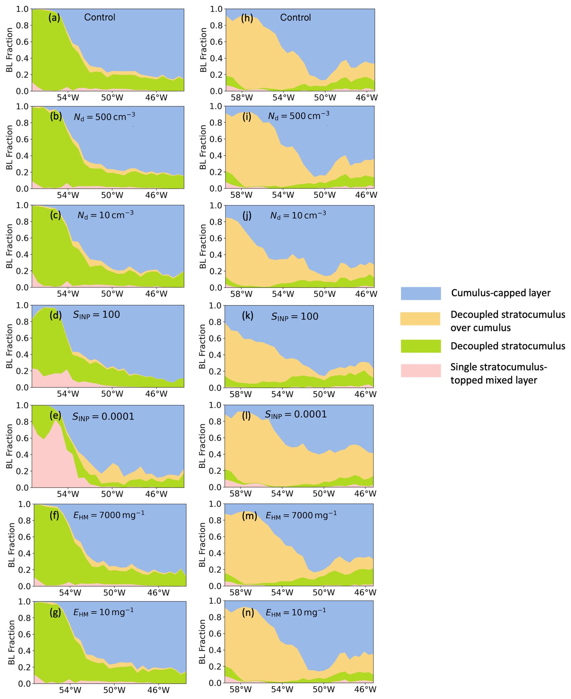
Figure G1 Boundary layer type fractions for all the simulations of 15 March 2022 (a–g) and 24 October 2022 (h–n). Four major boundary layer types are shown here: pink – single stratocumulus-topped mixed layer; green – decoupled stratocumulus; orange – decoupled stratocumulus over cumulus; and blue – cumulus-capped layer. Only pixels with cloud cover higher than or equal to 20 % are included for analysis.

Appendix H: Results of model simulations with different precipitation, evaporation, and sublimation setup for the March case

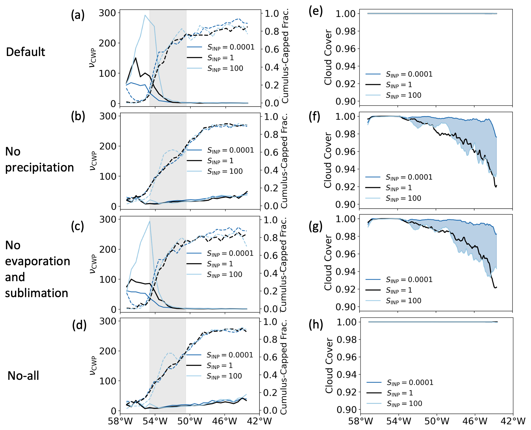
Figure H1 The cloud field homogeneity parameter (ν, solid lines) with the fraction of cumulus-capped boundary layer (dashed lines) in cloudy pixels (cloud cover ≥20 %) (a–d) and cloud cover (e–h) from simulations with perturbed S_INP for the (a, e) default setup, (b, f) no-precipitation (sedimentation of all hydrometeors) setup, (c, g) no-evaporation-and-sublimation setup, and (d, h) no-all (no precipitation, evaporation, and sublimation) setup for the March case.

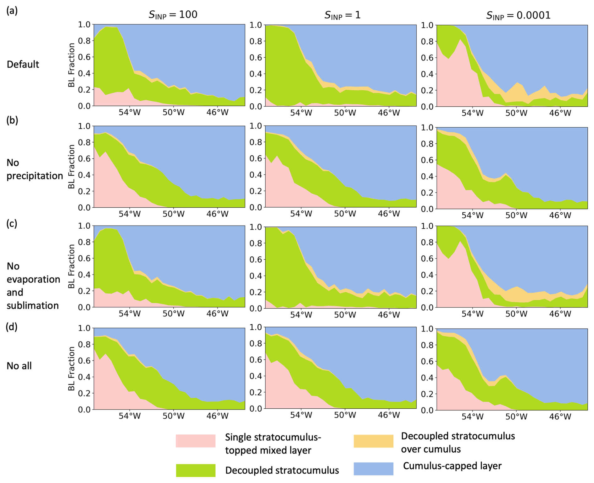
Figure H2 Boundary layer type fractions from simulations with perturbed S_INP for the (a) default setup, (b) no-precipitation (sedimentation of all hydrometeors) setup, (c) no-evaporation-and-sublimation setup, and (d) no-all (no precipitation, evaporation, and sublimation) setup for the March case.

Appendix I: Vertical profiles of in-cloud properties for simulations with different N_d and E_HM

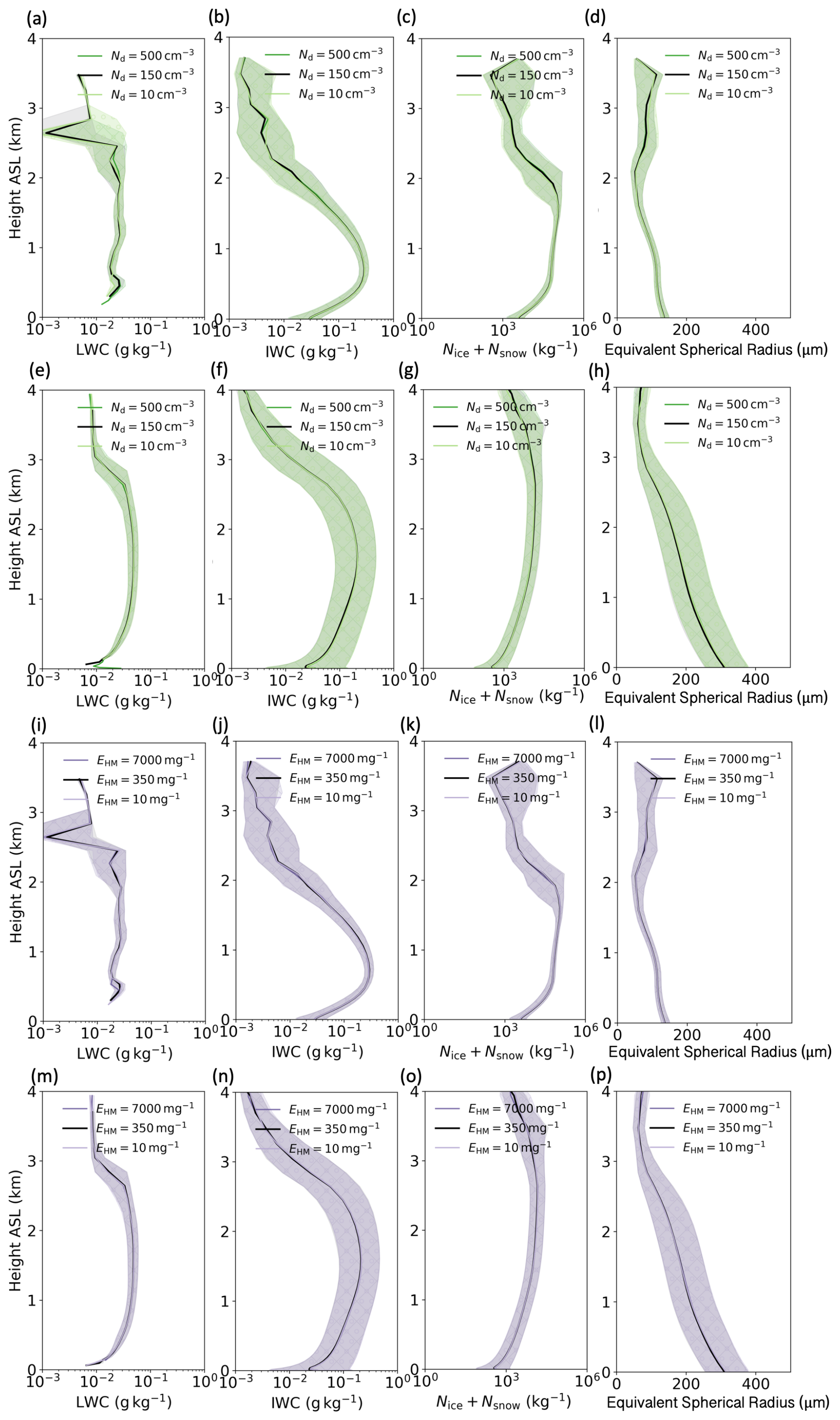
Figure I1 Vertical profiles of in-cloud LWC (liquid water content), in-cloud IWC (ice water content), N_ice+N_snow, and equivalent spherical radius for stratocumulus-dominated (a–d, i–l) and cumulus-dominated (e–h, m–p) regions in the 15 March 2022 CAO case with different N_d (a–h) and E_HM (i–p).

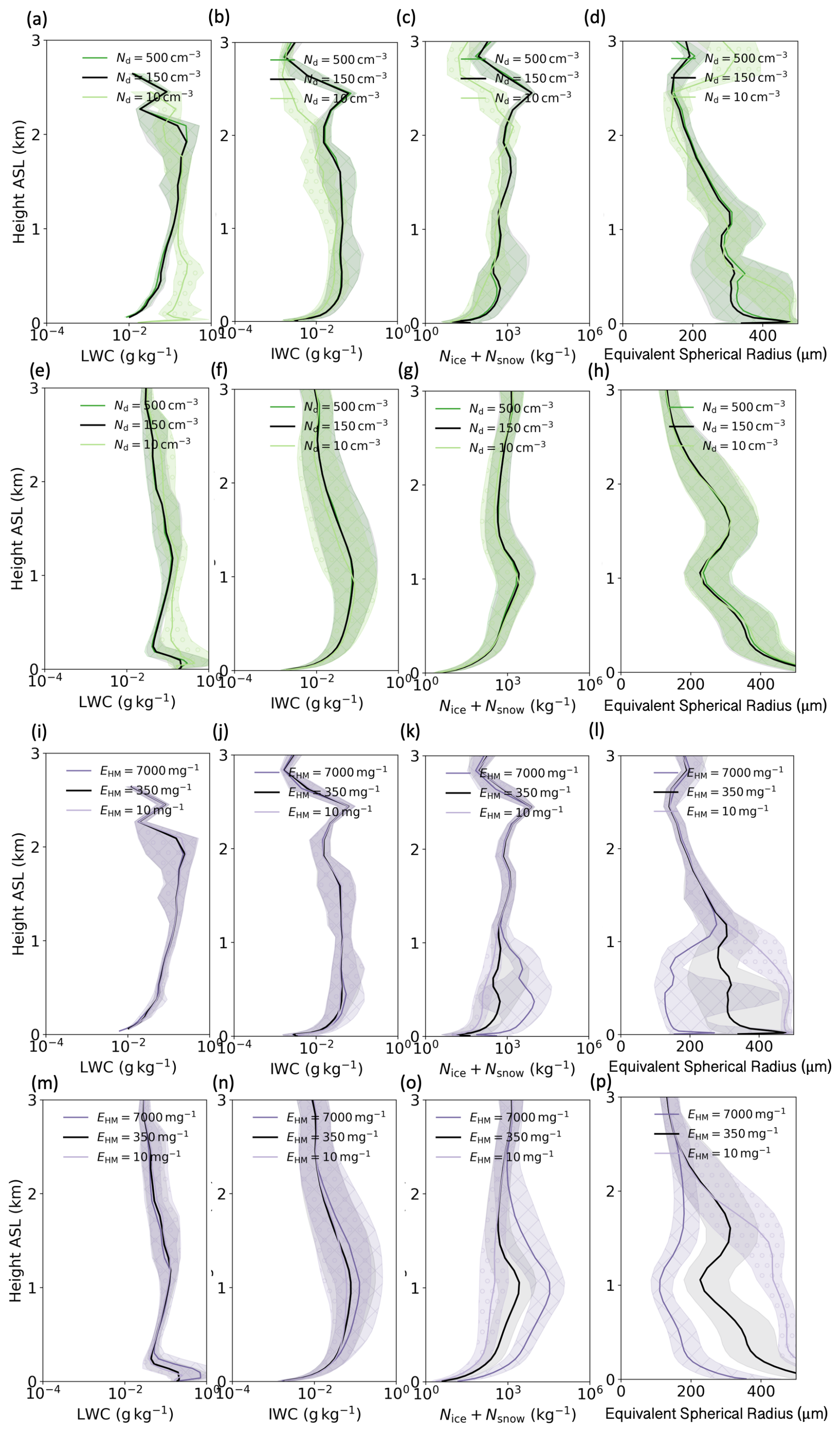
Figure I2 Vertical profiles of in-cloud LWC (liquid water content), in-cloud IWC (ice water content), N_ice+N_snow, and equivalent spherical radius for stratocumulus-dominated (a–d, i–l) and cumulus-dominated (e–h, m–p) regions in the 24 October 2022 CAO case with different N_d (a–h) and E_HM (i–p).

Appendix J: Supplementary figures for model output compared to satellite retrievals

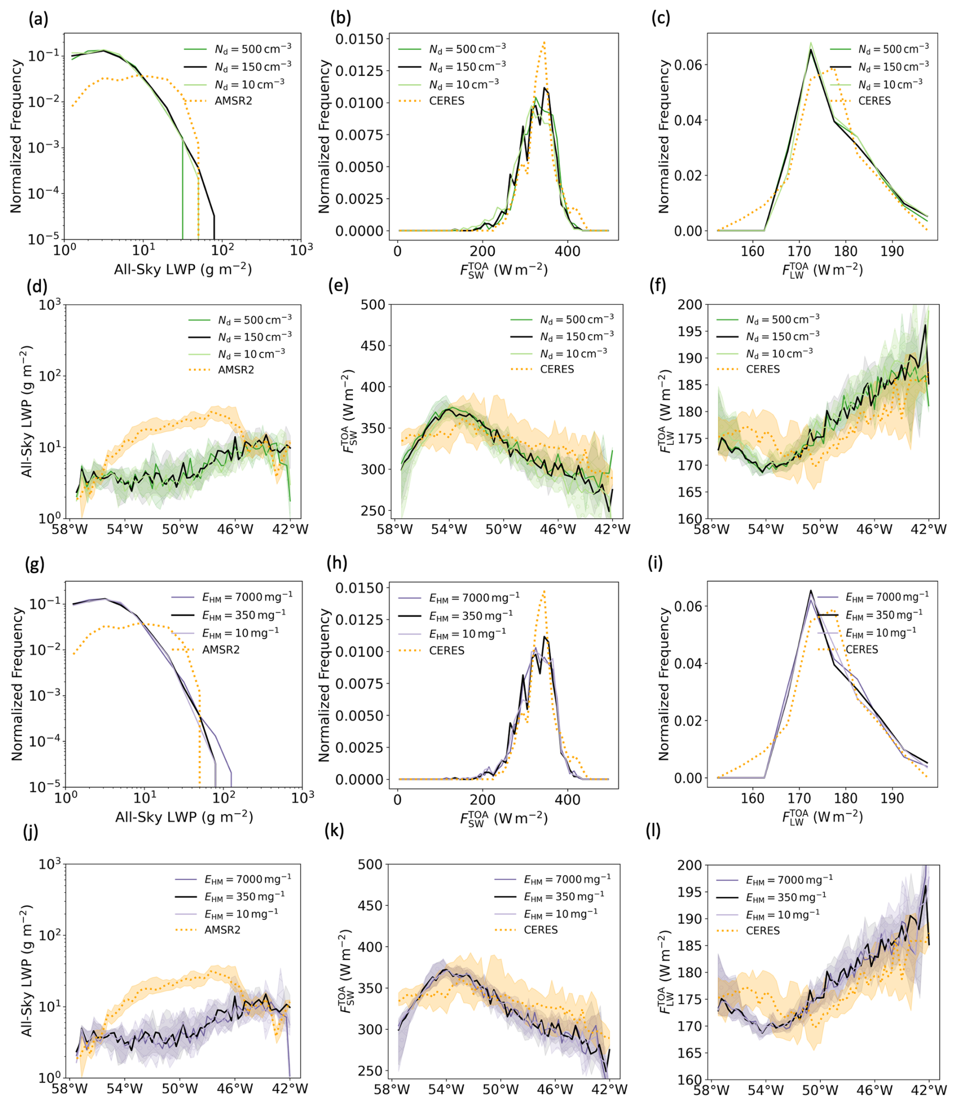
Figure J1 Model output compared with satellite retrievals for simulations with different N_d (a–f) and E_HM (g–l) on 15 March 2022: the normalized frequency of the all-sky liquid water path (LWP) from AMSR-2 (a, d, g, j) and the shortwave radiation at the top of the atmosphere (b, e, h, k) and longwave radiation at the top of the atmosphere (c, f, i, l) from CERES.

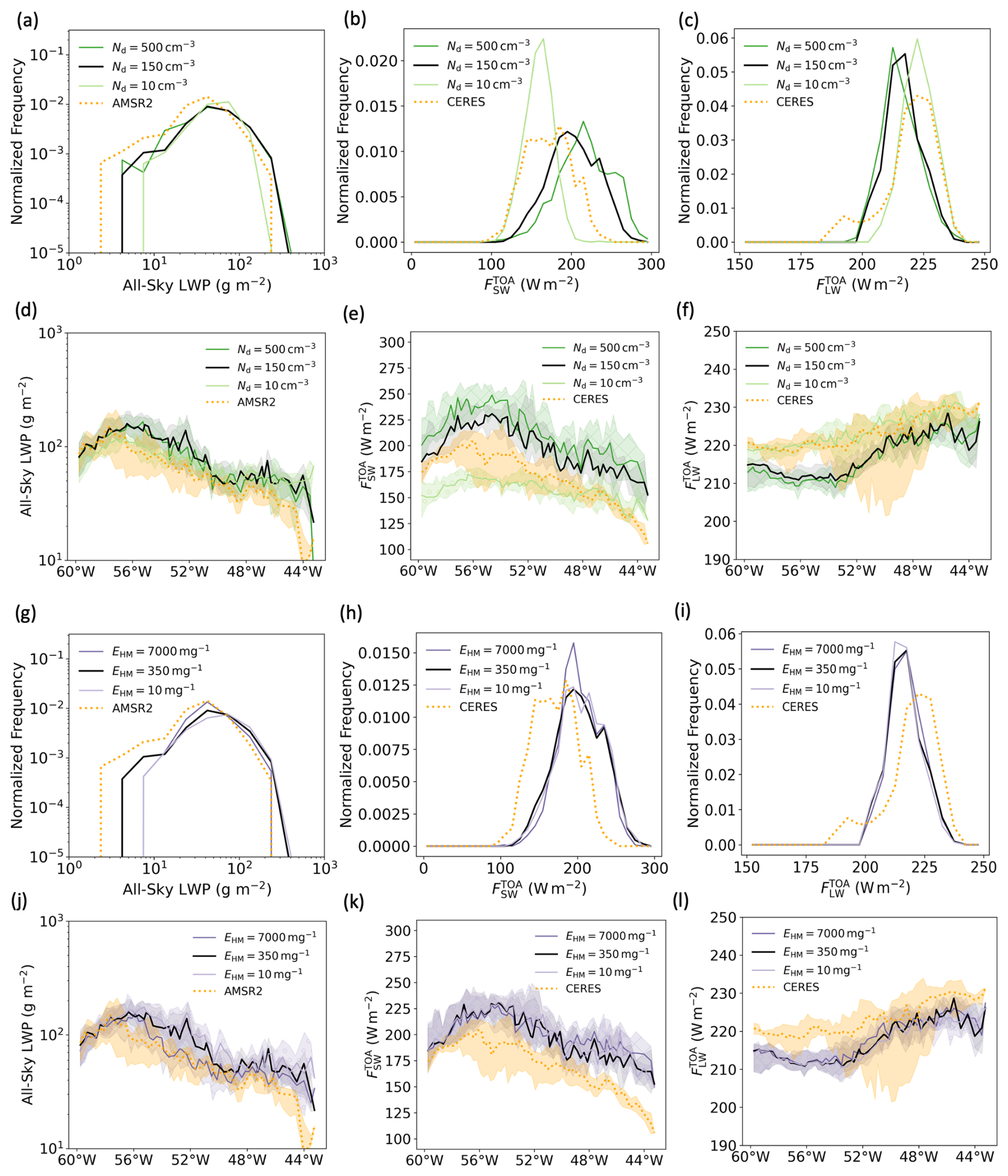
Figure J2 Model output compared with satellite retrievals for simulations with different N_d (a–f) and E_HM (g–l) on 24 October 2022: the normalized frequency of the all-sky liquid water path (LWP) from AMSR-2 (a, d, g, j) and the shortwave radiation at the top of the atmosphere (b, e, h, k) and longwave radiation at the top of the atmosphere (c, f, i, l) from CERES.

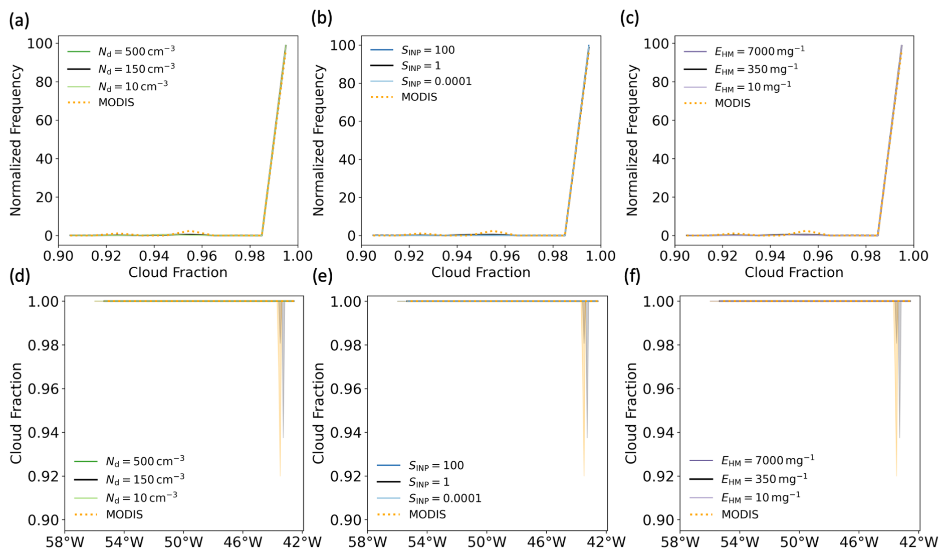
Figure J3 Modelled cloud fraction compared to the cloud fraction retrieved from MODIS on board the Aqua satellite with different N_d (a, d), S_INP (b, e), and E_HM (c, f) on 15 March 2022. Cloud fractions from the model were calculated using the percentage of model grids with cloud cover higher than 20 % in each coarser MODIS grid. Lines in (d), (e), and (f) are the cross-section medians, and the shaded area indicates the IQR (interquartile range).

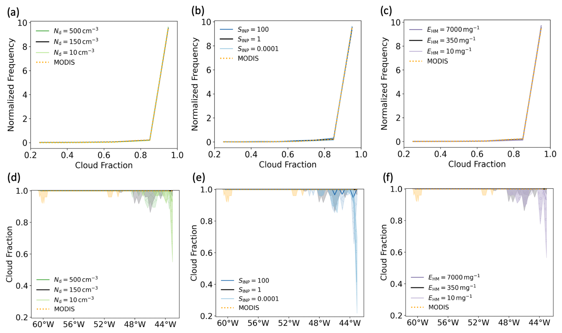
Figure J4 Modelled cloud fraction compared to the cloud fraction retrieved from MODIS on board the Aqua satellite with different N_d (a, d), S_INP (b, e), and E_HM (c, f) on 24 October 2022. Cloud fractions from the model were calculated using the percentage of model grids with cloud cover higher than 20 % in each coarser MODIS grid. Lines in (d), (e), and (f) are the cross-section medians, and the shaded area indicates the IQR (interquartile range).