High sensitivity of simulated fog properties to parameterized aerosol activation in case studies from ParisFog

Aerosols influence fog properties such as visibility and lifetime by affecting fog droplet number concentrations (N_d). Numerical weather prediction (NWP) models often represent aerosol–fog interactions using highly simplified approaches. Incorporating prognostic size-resolved aerosol microphysics from climate models could allow them to simulate N_d and aerosol–fog interactions without incurring excessive computational expense. However, microphysics code designed for coarse spatial resolution may struggle with sub-kilometer-scale grid spacings. Here, we test the ability of the UK Met Office Unified Model to simulate aerosol and fog properties during case studies from the ParisFog field campaign in 2011. We examine the sensitivity of fog properties to variations in N_d caused by modifications to simulated aerosol activation.

Our model, with a 500 m horizontal resolution and interactive aerosol and cloud microphysics, significantly underpredicts N_d, although it only slightly underestimates the cloud condensation nuclei concentration. With an updated version of the Abdul-Razzak and Ghan (2000) activation scheme, we produce N_d that are more consistent with those predicted by a cloud parcel model under fog-like conditions. We activate droplets only by adiabatic cooling. We incorporate more realistic hygroscopicities for sulfate and organic aerosols and explore the sensitivity of simulated N_d to unresolved updrafts. We find that both N_d and simulated fog liquid water content are very sensitive to the updated activation scheme but remain less affected by the update to hygroscopicities. Our improvements offer insights into the physical processes regulating N_d in stable conditions, potentially laying foundations for improved operational fog forecasts that incorporate interactive aerosol simulations or aerosol climatologies.

1 Introduction

Fog events are associated with reduced visibility that affects road, water, and air transportation. Behind freezing conditions, fog is the second leading cause of weather delays and cancelations at major airports across the United States (Goodman and Griswold, 2019). At Paris-Charles-de-Gaulle airport, the frequency of takeoffs and landings is reduced by half when visibility drops below 600 m due to fog (Roquelaure and Bergot, 2009). Therefore, accurate operational weather forecasts for fog are necessary.

Aerosol particles activate to form fog droplets, affecting visibility and fog life cycle (Stolaki et al., 2015; Boutle et al., 2018; Poku et al., 2019, 2021; Wainwright et al., 2021; Yan et al., 2021; Duplessis et al., 2021). These droplets, in turn, can influence light extinction, sedimentation, and evaporation rates (Ackerman et al., 2004; Hill et al., 2009) based on their concentration. Therefore, numerical weather prediction models are starting to use interactive prognostic aerosol microphysics schemes to improve the representation of aerosols and, therefore, better forecast fog (Jayakumar et al., 2021). In climate models, it is important to simulate droplet concentrations accurately in low-level clouds, which include different types of fog (for example, radiation fog or advection fog), in order to simulate the indirect effects of aerosols on climate. Since weather and climate models are becoming increasingly unified, consistent representations of aerosol–fog interactions that will work in both weather and climate models are desirable. If we can demonstrate that a comprehensive prognostic aerosol scheme can improve simulations, it would then be possible to test possible simplifications that would save computational expense for specific operational settings, for example, using aerosol climatologies.

However, while low clouds have much in common with fog, there are also important differences, especially in how aerosols affect clouds and fog. For the same aerosol concentration, fog droplet concentrations (N_d) are expected to be lower than droplet concentrations in clouds. The main physical reason for the low N_d is that in fog, updraft speeds are generally lower than in clouds, reducing aerosol activation rates. Activation is likely to occur at least in part due to radiative cooling (Gultepe et al., 2007; Wærsted et al., 2017; Poku et al., 2021) rather than vertical air motion.

In this study, we improve the simulated fog droplet number concentration in the UK Met Office Unified Model (UM) for fog cases observed near Paris in 2011. We were inspired by several previous specific studies: for example, using a single column model Stolaki et al. (2015) found that doubling the number of cloud condensation nuclei concentration (CCN) in a subset of the days we use in our case study from the ParisFog campaign led to a 60 % increase in the liquid water path. Simulating actual supersaturation and condensational growth of aerosols in a large eddy simulation (LES) model Boutle et al. (2018), found that the onset of well-mixed fog (in which the vertical profile of liquid water content (LWC) is near adiabatic) was dependent on aerosol activation. The interaction of the land surface with radiation led to the initial fog formation, while the fog layer itself started interacting with radiation only when a substantial fraction of the population of the largest aerosols was activated, resulting in optically thicker fog. WRF-Chem modeling studies by Yan et al. (2021) and Jia et al. (2019) found that an increase in the number of cloud condensation nuclei concentrations could advance fog formation, delay fog dissipation (by about an hour), enhance fog intensity, and generate long and severe fog events. An LES study by Vié et al. (2024) found that significant improvements in simulations of fog in the UK could be achieved by modifying the cooling rates used in aerosol activation, which were previously overestimated. The high sensitivity of fog properties, including even thermodynamic profiles, to the simulated cooling rates used in the activation scheme also highlights the importance of aerosol–fog interactions.

Weather and climate models that represent aerosols prognostically (e.g., Jayakumar et al., 2021; Lohmann, 2002) use aerosol activation parameterizations as the source of cloud and fog droplets. The parameterizations typically balance a source of supersaturation, usually only adiabatic cooling due to updrafts, with a sink due to condensation on activating aerosol particles. The parameterizations are needed because changes in supersaturation generated by updrafts typically occur on timescales of a few seconds, too short to be explicitly resolved by large-scale models. The widely used Abdul-Razzak and Ghan (2000) activation scheme, henceforth “ARG”, was originally developed for boundary layer stratiform clouds and can also be applied to cumulus clouds (Ghan et al., 2011). It calculates N_d from cooling due to vertical air motion, temperature, the aerosol size distribution, and their hygroscopicity. Similarly to most climate models, many cloud-resolving scale modeling studies, including those of fog, use the ARG activation scheme (e.g., Chapman et al., 2009; Jia et al., 2019). However, the parameterization of visibility in numerical weather prediction models is sometimes an exception in that the ARG scheme is not always used. In the UM, for example, visibility is parameterized as a function of aerosol mass loading and relative humidity, via a scheme that is similar to a simplified diagnostic representation of aerosol activation (Clark et al., 2008) that does not depend on vertical air motion. However, this parameterization assumes that the aerosols are monodisperse. If possible, it would be preferable to calculate the visibility of the prognostic N_d and LWC from a cloud microphysics parameterization that handled all types of clouds, including fog, with a consistent activation scheme that considers aerosol properties such as size and hygroscopicity.

To represent the cloud microphysics of fog in a weather prediction or climate model, several other assumptions are also needed. One important assumption is that the fog size distribution has a single droplet mode, as these models generally have “bulk microphysics schemes” without size sections or multiple modes for cloud droplets. However, two droplet modes, both below 30 µm in diameter, are frequently observed during fog (Mazoyer et al., 2022). The error in approximating the fog droplets with a single mode remains to be quantified. Related to this is the assumption that unactivated haze aerosols and droplets are distinct entities. The wet critical diameter (threshold diameter of a wet particle beyond which it can grow spontaneously and form a droplet) can be around 3–5 µm (Mazoyer et al., 2022), a factor of 10 greater than the dry critical diameter (threshold diameter of a dry aerosol before condensation, beyond which spontaneous growth happens) (Mazoyer et al., 2019). Bulk aerosol microphysics coupled to bulk cloud microphysics schemes are well known to struggle to fully capture the details of the activation and deactivation of haze (Yang et al., 2023), long recognized as a difficult problem in cloud modeling (e.g., Árnason and Brown, 1971). This is especially challenging without representing complex mixing interactions or accounting for surface tension changes due to surfactants. A key aim of this paper is to examine whether bulk microphysics is nonetheless a sensible pragmatic solution for modeling aerosol–fog interactions despite these shortcomings.

Here, we use a regional configuration of the Unified Model to investigate aerosol activation in case studies of fog over Paris. Similar simulation systems are used for the operational forecasting of fog over London (Boutle et al., 2016) and Delhi (Jayakumar et al., 2021), although the published systems did not use double-moment cloud microphysics. We use observational data from the ParisFog field campaign (Haeffelin et al., 2010) at the Instrumented Site for Atmospheric Remote Sensing Research (SIRTA) in November 2011. The occurrence of 11 fog cases in two weeks with detailed observations of aerosol and fog microphysics makes the campaign preferred for our study (although other field campaigns such as LANFEX in the UK (Price et al., 2018) or WiFEX in New Delhi (Ghude et al., 2017) could also have been used). In this paper, we simulate fog N_d using adiabatic cooling as a source of supersaturation, in a 500 m resolution simulation with double-moment aerosol and cloud microphysics, nested inside lower-resolution simulations. We focus on improving the parameterization of activation without changing the fundamental mechanism of supersaturation generation by adiabatic cooling. Although it is likely that adiabatic cooling is not the dominant source of supersaturation in all the fog cases we study, adiabatic cooling is the simplest and most widely used approach to activation in models.

We evaluate simulated aerosol and fog droplet concentrations using the ParisFog observations and test the existing activation scheme in our model. We discuss the observational data and details of several instruments in Sect. 2. The setup of our model is discussed in Sect. 3. Section 4 explains our model developments that affect N_d in fog. In Sect. 5, we discuss the model evaluation and the results. Finally, in Sect. 6, we present our conclusions.

In the companion paper (Ghosh et al., 2025c), we examine more exploratory model developments. We add radiative cooling as a source of supersaturation in the ARG scheme and study the fog life cycle simulated by the model. We also design several sensitivity studies to address missing sinks and model artifacts that might affect the droplet budget in the model. Finally, we calculate the relative importance of the adiabatic and radiative cooling components of activation in the droplet budget.

2 Measurements and case study

In this study, we use measurements from the ParisFog field campaign to evaluate our model. ParisFog refers to several field campaigns that have taken place since 2006 at the Instrumented Site for Atmospheric Remote Sensing Research (SIRTA) to understand the life cycle of fog. Haeffelin et al. (2005) describe the SIRTA observatory (48.713° N, 2.208° E), located near the Ecole Polytechnique Palaiseau, on the Saclay plateau at 160 m above sea level, about 20 km southwest of the Paris city center, which is mostly around 35 m above sea level. The site is located in a semi-urban environment composed of roughly equal portions of agricultural fields, wooded areas, housing, and industrial developments. Prevailing winds advect clean air from the Atlantic Ocean towards the site. Winds from the northeast carry pollutants from the Paris metropolitan area, affecting the aerosol composition over SIRTA.

We show observations of 11 fog events between 15 and 25 November 2011 in this paper. Mazoyer et al. (2019) categorizes the four fog events on 16 (afternoon), 24 (morning and afternoon), and 25 November as stratus lowering, and the remaining events on 15, 16 (morning), 18, 19, 21, 22, and 23 November as radiation fogs. The microphysical properties of the droplets and aerosols were measured regularly using different instruments. The details of all the instruments and their setup used during the ParisFog campaign are well documented in previous studies (Hammer et al., 2014; Stolaki et al., 2015; Elias et al., 2015; Dupont et al., 2016; Mazoyer et al., 2017, 2019, 2022); those we use here are listed in Table 1. To evaluate simulated meteorology, we use near-surface temperature and relative humidity data from the weather sensors at SIRTA (48.7° N, 2.2° E) and Trappes (48.7° N, 2° E). We also use a regional weighted average of measurements from Trappes, Orly (48.7° N, 2.4° E), and Paris Montsouris (48.8° N, 2.3° E), following Sect. 3.2.1 of Chiriaco et al. (2018). We also use the vertical profiles of temperature and relative humidity from radiosondes launched by Météo-France twice a day from Trappes, situated 15 km northwest of the SIRTA observatory.

Table 1 Instruments used to measure optical, radiative, and microphysical properties of aerosols and droplets during the ParisFog field campaign that we also use in our model evaluation. n/a: not applicable.

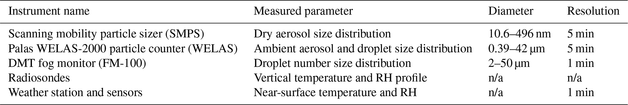
The dry aerosol number size spectrum was measured using a scanning mobility particle sizer (SMPS). The instrument was placed inside a shelter. Air was sampled and passed through an aerodynamic size discriminator PM_2.5 inlet and then through a dryer, reducing the relative humidity to less than 50 %. The differential mobility analyzer (DMA; TSI 3071) in the SMPS that selected particles from 10.6 to 496 nm in diameter had hydrophilic filters lowering the relative humidity to less than 30 %  (Denjean et al., 2014), which is the point at which we can neglect water uptake by typical urban aerosols (e.g., Seinfeld and Pandis, 1998). The size distribution of larger particles at ambient relative humidity was measured using two optical spectrometers: the WELAS-2000 (Palas GmbH, Karlsruhe, Germany) and the fog monitor FM-100 (Droplet Measurement Technologies Inc., Boulder, CO, USA). The WELAS-2000 (hereafter referred to as WELAS) is designed to measure particles within 0.4 and 40 µm in diameter, but previous studies found that the detection efficiency decreases drastically below 1 µm (Heim et al., 2008; Elias et al., 2015). Hammer et al. (2014) used data with diameters larger than 1.4 µm and Mazoyer et al. (2019) used 0.96 µm as a threshold diameter. The FM-100 fog monitor provides droplet size distribution from 2 to 50 µm in diameter, thus having a large overlap with the WELAS. However, comparisons by Burnet et al. (2012) and  Elias et al. (2015) show that distributions from these instruments overlap only from 5–9 µm diameter, because the FM-100 overestimated particles lower than about 5 µm while the WELAS underestimated droplets larger than 10 µm (Burnet et al., 2012; Elias et al., 2015). Figures 1 and A1 of Mazoyer et al. (2019) demonstrate the bias. In our work, we plot the overlapping range from both instruments. The FM also provides LWC in the fog.

3 Model description

3.1 Meteorological model

We use UM version 13.0 to study aerosol activation and aerosol–fog interaction. To enable prognostic aerosol and cloud microphysics, simulations are run within the NUMAC (Nested Unified Model with Aerosols and Chemistry) system (Gordon et al., 2023). The coupling of the double moment cloud microphysics (Field et al., 2023) to the double moment aerosol microphysics (Mulcahy et al., 2020) is described by Gordon et al. (2020). We use three different configurations of the model: a global model, a 4 km grid resolution regional model nested within it, and a 500 m grid resolution regional model nested within the 4 km model. The nesting is “one-way”: the coarser resolution domains provide lateral boundary conditions to the finer-resolution domains. The regional models use time steps of 120 and 30 s for the dynamics, respectively, with a common chemistry time step of 120 s.

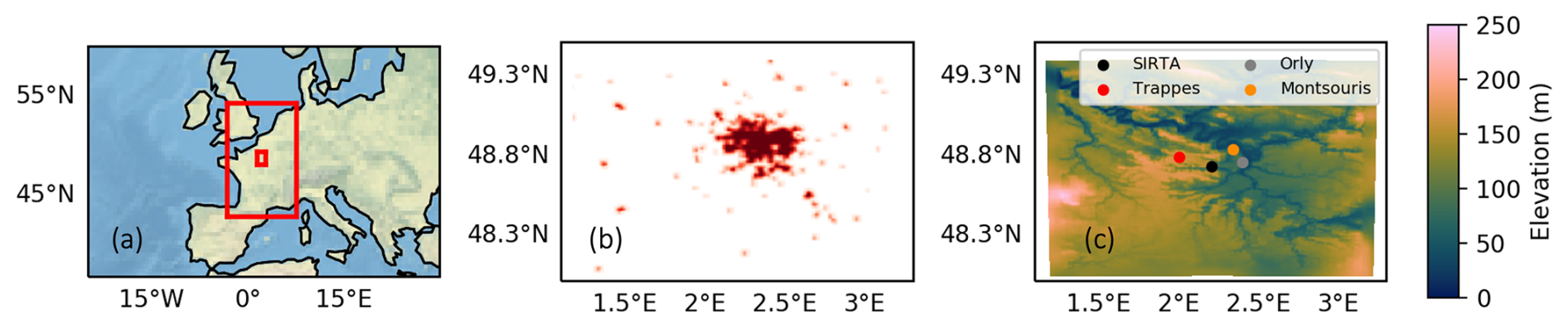
Figure 1 (a) Location of the two regional nested domains used in this study is shown. Both the domains are centered over the SIRTA observatory near Paris. The outer domain has 4 km grid resolution and the inner domain has 500 m resolution. Both the domains have 300 grid points in the latitude and longitude directions. (b) Urban grid cells in the 500 m resolution model domain. The regional scale is set by Paris near the center and Chartres in the southwest at approximately 48.44° N, 1.49°E. (c) Surface altitude (m) in the 500 m resolution domain is shown here. Measurement sites at SIRTA observatory (domain center), Trappes (radiosondes), and Orly and Paris Montsouris (weather stations) are shown by colored dots.

This work focuses primarily on results from the regional 500 m resolution model. The 500 m model is centered over the SIRTA observatory, as shown in Fig. 1a. Figure 1b shows the urban grid cells in the 500 m resolution model (roughly the area of Paris city) and subfigure Fig. 1c shows surface elevation (m) in our 500 m resolution domain. The SIRTA observatory (the domain center), Trappes (location of radiosondes, discussed later), and Orly and Paris Montsouris (weather stations, discussed later) are shown by colored dots. We use 300 grid points in both latitude and longitude directions in both our 500 m and 4 km resolution domains, with 70 vertical levels extending up to 40 km. These domains use the Regional Atmosphere and Land Version 3 (RAL3) physical atmosphere model configuration (Bush et al., 2025), which is similar to Regional Atmosphere and Land Version 2 (Bush et al., 2023) but with the two moment Cloud–AeroSol Interacting Microphysics (CASIM) scheme (Shipway and Hill, 2012; Grosvenor et al., 2017; Field et al., 2023) used by default in place of the single moment microphysics scheme of Wilson and Ballard (1999). In Sect. 3.2, we describe the microphysics schemes in detail. The RAL3 configuration also uses the more recently developed cloud fraction scheme of Van Weverberg et al. (2021) by default; however, we found that the cloud cover was underpredicted with this scheme and that this prevented a robust model evaluation of cloud properties. The underprediction of cloud cover in the bimodal scheme is discussed in more detail by Van Weverberg and Morcrette (2022), who compare all the cloud schemes available in the UM. Therefore, in this work, we used the sub-grid cloud fraction scheme by Smith (1990), which is better able to generate cloud when supersaturations are low, as in fog. The gray-zone turbulence parameterization of Boutle et al. (2014) is used to represent subgrid-scale mixing in the boundary layer within the boundary layer scheme described by Lock et al. (2000). The model uses the ENDGAME semi-Lagrangian dynamical core (Wood et al., 2014; Thuburn, 2016) and no parameterized convection. Radiative transfer is treated by the SOCRATES scheme (Manners et al., 2015) based on work by Edwards and Slingo (1996).

The global model has a horizontal resolution of 1.87°×1.25° (labeled N96 within the UM framework) with 85 vertical levels extending up to 85 km from the surface. It uses the same code base as the regional model, but because the global model uses the global atmosphere science configuration GA7.1 (Walters et al., 2019), which differs from the RAL3 configuration, there are differences between the settings of various parameters in the simulations of dynamics, boundary layer, radiation, and sub-grid cloud. The most important difference for this work is that the configuration stipulates that the PC2 (Prognostic Cloud, Prognostic Condensate) sub-grid cloud scheme (Wilson et al., 2008) be used in the global model instead of the Smith or bimodal schemes and that convection is parameterized in the global model.

To ensure the simulated meteorology closely follows reality, the regional model is initialized at 12:00 UTC on each day from 14 to 25 November and run for 28 h each time. We used the UK Met Office global weather forecast fields, available at high resolution (∼12 km), to initialize meteorological variables such as temperature, wind speed, and humidity in the nested regional models. These global weather forecasts closely follow real meteorology because they are generated with data assimilation; however, we do not use data assimilation in our own simulations to avoid complicating the interpretation of our results. The concentrations of chemistry and aerosol species are not represented in the global forecast, so they are carried forward from the previous forecast as described by Gordon et al. (2023). The aerosol and chemistry fields at the start of the simulation on 14 November are initialized from a nudged global simulation with a configuration similar to the atmosphere-only UKESM1 model (Mulcahy et al., 2020; Sellar et al., 2020).

Results from the first 4 h of each forecast simulation are discarded to allow simulated low clouds and fog in the initialization files to adjust to the higher spatial grid resolution and aerosol concentrations in our model. We expect that 4 h is an adequate spin-up time, first because fog is rarely observed during the spin-up period (12:00–16:00 UTC), and second because, even when it is present, we expect that N_d at any given time is independent of N_d four hours earlier. We acknowledge that this may not be enough time to fully represent adjustments of cloud liquid water path to aerosol (e.g., Glassmeier et al., 2021).

3.2 Chemistry, aerosol, and cloud microphysics

We use the StratTrop chemistry scheme within the UK Chemistry and Aerosol (UKCA) submodel (Archibald et al., 2020; Gordon et al., 2023) in this study. This complex scheme, with 84 chemical tracers and 291 reactions, is required to simulate nitrate aerosols, which are an important component of total aerosol mass in Paris (Crippa et al., 2013; Roig Rodelas et al., 2019). In the regional models, the most important difference arises from the lack of convection parameterization, which means NO is not produced from lightning by default. To address this problem, the lightning flash rate parameterization of McCaul et al. (2009) was used in our study, as in Gordon et al. (2023). Updates to the simulated sulfur cycle described by Mulcahy et al. (2023) are also included.

This study uses the double moment modal Global Model of Aerosol Processes (GLOMAP-mode, hereafter referred to as GLOMAP) aerosol microphysics scheme (Mann et al., 2010; Mulcahy et al., 2020) within UKCA, including the improvements of Mann et al. (2012) and the changes recommended by Mulcahy et al. (2018). Different aerosol species are represented by 5 log-normal modes, labeled nucleation soluble, Aitken soluble, Aitken insoluble, accumulation soluble, and coarse soluble by Mann et al. (2010). Mineral dust is treated separately by the CLASSIC (Coupled Large-scale Aerosol Simulator for Studies In Climate) sectional scheme of Woodward (2001). All aerosol and most chemical species are transported by the Unified Model's semi-Lagrangian advection scheme. For the first time in the UM regional modeling configurations, our work also includes ammonium and nitrate aerosols along with black carbon, organic carbon, sea salt, and sulfate, following Jones et al. (2021). These chemical species are assumed to be internally mixed within the lognormal modes. Each mode has a fixed “width” or geometric standard deviation, but the median diameter is calculated from the independent, prognostic mass and number concentrations. The width of the accumulation mode is set to 1.4, based on a comparison with a sectional model and a review of the observational literature by Mann et al. (2012).

The Coupled Model Intercomparison Project (CMIP6) inventory (Feng et al., 2020) is used for anthropogenic and natural aerosol emissions in the global model. The high-resolution Emission Database for Global Atmospheric Research, developed to assess Hemispheric Transport of Air Pollutants (EDGAR-HTAP), is used for anthropogenic emissions in the regional model (Janssens-Maenhout et al., 2015). EDGAR-HTAP provides monthly global anthropogenic emissions at 0.1°×0.1° horizontal resolution (for 2010). Non-anthropogenic and biomass burning emissions for the regional model are not included in the EDGAR inventories, so are taken from the CMIP6 inventories used by the global model instead. These datasets are used after regridding to the resolution of the global model to avoid additional processing.

Different cloud microphysics schemes are used for different configurations in our study. The single-moment scheme of Wilson and Ballard (1999) is used in the global model. This scheme uses only the mass of hydrometeors as prognostic variables. However, we use the two-moment CASIM microphysics scheme in our regional domains to simulate the life cycle of fog. In CASIM microphysics cloud, rain, ice, snow, and graupel are represented by separate gamma distributions. We follow Field et al. (2023) in using a shape parameter of 2.5 in the cloud droplet size distribution, which is an update from the 5.0 used by Gordon et al. (2020). Condensation of water vapor onto cloud droplets is represented with the “saturation adjustment” assumption, which means supersaturation is not prognostic and droplets are assumed to be in equilibrium at the end of each model time step. In the regional model, the onset of non-zero fractional cloud cover starts when the grid mean relative humidity exceeds 96 % to account for sub-grid variability, as discussed in Boutle et al. (2016). Liquid water content is passed from the 4 km resolution model to the 500 m model through the boundaries, while the N_d at the boundaries is kept constant at 100 cm⁻³. The coupling of CASIM to the GLOMAP aerosol scheme is described by Gordon et al. (2020). Aerosol number concentration in the soluble Aitken, accumulation, and coarse modes, and the diameters and volume-weighted hygroscopicities of these modes are passed from the aerosol code to the activation scheme in the cloud microphysics code.

In all configurations of our model, the Abdul-Razzak and Ghan (ARG) activation parameterization (Abdul-Razzak and Ghan, 2000) is used to activate aerosols at cloud base or when new cloud forms. This scheme was also used successfully for fog by Jia et al. (2019) and Yan et al. (2021) in WRF-chem and by Poku et al. (2019) with the CASIM microphysics scheme in a large eddy simulation. The ARG parameterization calculates N_d based on the aerosol size distribution and on the change in ambient supersaturation, which relies only on updraft speeds to generate cooling in this paper (radiative cooling is introduced in the companion paper). Above the cloud base in existing clouds, the supersaturation is determined from a balance assuming a steady-state between a source (adiabatic cooling due to ascent) and the sink to existing cloud droplets (Gordon et al., 2020). Since there is a sub-grid cloud fraction scheme, both this approach and the ARG activation parameterization can be active in the same grid box.

Aerosol activation is simulated whenever there is a tendency for water vapor to condense rather than evaporate. At each time step, if the activation scheme is called, it updates the N_d if the N_d calculated at that time step exceeds the N_d that existed in the grid box before the activation scheme was run. We believe this procedure was first introduced by Clark (1974) and is commonly used in regional and global weather and climate models (e.g., Lohmann, 2002). As a result, we expect that N_d depends on the highest updraft speed the model simulates since the formation of the cloud or fog in an air parcel, as well as other processes such as sedimentation and advection.

The default model configuration uses a minimum updraft speed of 0.01 m s⁻¹ in the activation scheme (so any updraft speeds lower than this are set to 0.01 m s⁻¹ for activation when the criteria described in the next paragraph are met). In this study, most of our simulations use the resolved, grid-average, updraft speed in the ARG activation scheme, with no representation of sub-grid turbulence. This practice is frequently used in other cloud-resolving models (for horizontal grid resolutions at or below 1 km), such as the Regional Atmospheric Modeling System, RAMS (Saleeby and Cotton, 2004), and was used in the paper describing CASIM in the UM Field et al. (2023). However, sub-grid turbulence is likely an important source of updrafts for the activation of aerosols in fog. Despite earlier work (Malavelle et al., 2014; Gordon et al., 2020), we do not yet have a robust approach to represent sub-grid-scale updraft speeds across all cloud types, including fog, or across varying model grid resolutions. Addressing this limitation fully requires a dedicated, comprehensive study. Nevertheless, in this paper, we conduct two additional simulations to understand the possible effects on simulated N_d of including a realistic contribution from sub-grid-scale turbulence to updrafts in activation.

In the CASIM microphysics as described by Field et al. (2023), the activation scheme is called when the LWC in a grid box increases, but droplets deactivate only if cloud fraction decreases, irrespective of LWC. For consistency, we instead choose to call the activation scheme when the cloud fraction remains the same (for example, in 100 % foggy grid boxes) or increases, and is not dependent on a change in the LWC. We include this change in all of our simulations. Usually, changes in LWC correlate with changes in cloud fraction, so we expect this change to have minimal effects on N_d.

Abdul-Razzak and Ghan (2000)Abdul-Razzak and Ghan (2000)Mann et al. (2010, 2012)Mann et al. (2010, 2012)Wilson et al. (2008)Smith (1990)Wilson and Ballard (1999)Field et al. (2023)Feng et al. (2020)Janssens-Maenhout et al. (2015); Feng et al. (2020)Manners et al. (2015)Manners et al. (2015)Lock et al. (2000)Boutle et al. (2014)Walters et al. (2019)Bush et al. (2025)

Table 2 Summary of parameterizations used in the global and regional models.

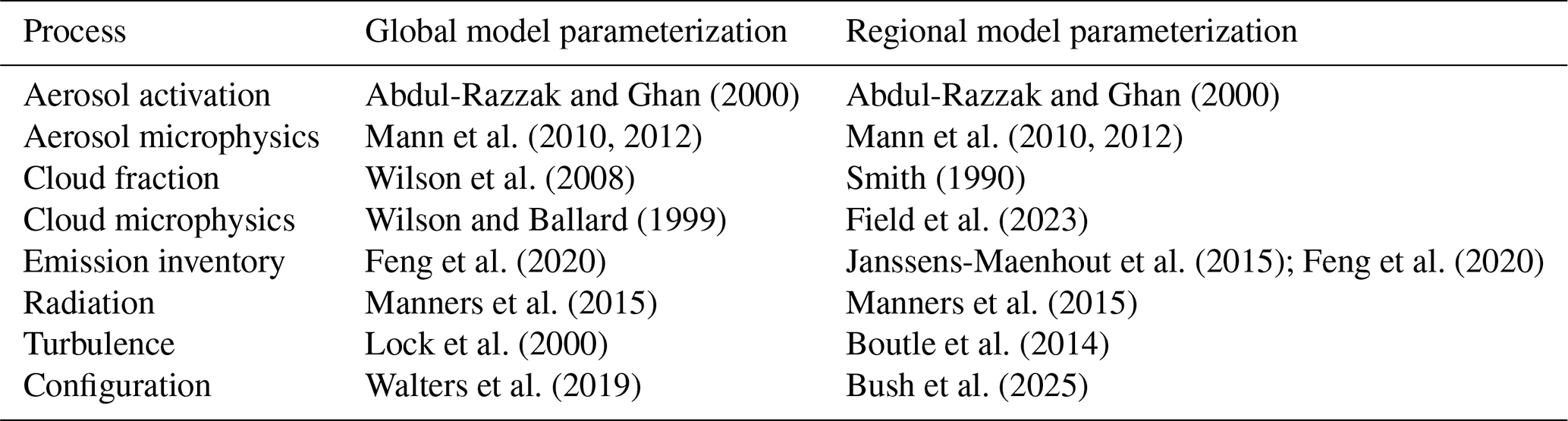
Aerosols are not removed or advected separately when they activate into droplets. Hence, in-cloud processing of aerosols is not represented, although sulfate mass does increase via aqueous chemical reactions, depending on LWC and concentrations of sulfur dioxide, hydrogen peroxide, and ozone. Aerosols are only removed irreversibly during significant rain or snow, depending on the autoconversion and accretion rates through which cloud droplets are converted to precipitation, as described by Mulcahy et al. (2020). In our simulations, therefore, aerosols in fog droplets are only removed via dry deposition; including an enhancement to aerosol removal due to the faster sedimentation rates of droplets compared to aerosol particles could be useful for future development. In Table 2, we provide a brief summary of different parameterizations used in this study.

4 Testing improvements to simulated activation due to adiabatic cooling

4.1 Default ARG scheme (Def-ARG)

In our default simulation, termed Def-ARG hereafter, we use the ARG scheme with in-cloud activation (as described earlier) to examine whether the parameterization developed for clouds can simulate fog realistically.

4.2 ARG scheme with adjusted parameters (Mod-ARG)

The semi-empirical ARG scheme for aerosol activation was not, as far as we know, designed for the low updrafts observed in fog (Abdul-Razzak and Ghan, 2000; Ghan et al., 2011), where the effect of the kinetic limit on the rate of water uptake during activation can often become important, especially in polluted conditions. These kinetic limitations are not accounted for in the ARG parameterization (Nenes et al., 2001; Phinney et al., 2003), though they are in some more sophisticated alternatives (e.g., Morales Betancourt and Nenes, 2014). Furthermore, when comparing predictions of the ARG parameterization to the Pyrcel cloud parcel model of Rothenberg and Wang (2016), we found it exhibits significant biases for the geometric standard deviation of the accumulation mode used in GLOMAP, 1.4, which is smaller than the value used in most other modal aerosol microphysics schemes.

In the ARG activation scheme, activated N_d are calculated from maximum supersaturation S_max. The expression for S_max is the following:

$$\begin{array}{}\text{(1)}& S_{\text{max}}={\left\{\sum _i{\displaystyle \frac{\mathrm{1}}{S_{mi}^{\mathrm{2}}}}\left[f_i{\left({\displaystyle \frac{\mathit{\zeta }}{{\mathit{\eta }}_i}}\right)}^p+g_i{\left({\displaystyle \frac{S_{mi}^{\mathrm{2}}}{{\mathit{\eta }}_i+\mathrm{3}\mathit{\zeta }}}\right)}^{\mathrm{3}/\mathrm{4}}\right]\right\}}^{-\frac{\mathrm{1}}{\mathrm{2}}},\end{array}$$

where i indexes aerosol modes in a multi-modal lognormal size distribution and $p=\mathrm{3}/\mathrm{2}$.

The empirical parameters f and g, are functions of aerosol mode width σ. S_max depends on the critical supersaturation S_m of a particular mode and two non-dimensional parameters η and ζ which are functions of updraft speed, surface tension and thermodynamic parameters, and are independent of the widths of the size modes. Following Eq. (6) in Abdul-Razzak and Ghan (2000), for each aerosol mode, f and g were determined by comparison to a parcel model as

$$\begin{array}{ll}{\displaystyle }{f}_i& {\displaystyle }=\mathrm{0.5}\exp \left(\mathrm{2.5}{\ln }^{\mathrm{2}}{\mathit{\sigma }}_i\right)\\ \text{(2)}& {\displaystyle }{g}_i& {\displaystyle }=\mathrm{1}+\mathrm{0.25}\ln {\mathit{\sigma }}_i.\end{array}$$

Lower values of f and g would lead to higher activation fraction (higher N_d). In a separate study (Ghosh et al., 2025a), we determined improved values of f and g by comparing the parameterization to the Pyrcel model simulations. We also determined a modified value of p which substantially improves the performance of the scheme in cases where kinetic limitations to droplet activations are critical. We use the following modified equations to reduce biases in N_d predicted by the parameterization:

$$\begin{array}{ll}{\displaystyle }f& {\displaystyle }=\mathrm{0.0135}{e}^{\mathrm{2.367}{\mathit{\sigma }}_{\text{acc}}}\\ {\displaystyle }g& {\displaystyle }=\mathrm{1.1058}-\mathrm{0.315}{\mathit{\sigma }}_{\text{acc}}\\ \text{(3)}& {\displaystyle }p& {\displaystyle }=-\mathrm{0.5073}+\mathrm{1.5088}{\mathit{\sigma }}_{\text{acc}}-\mathrm{0.3699}{\mathit{\sigma }}_{\text{acc}}^{\mathrm{2}}.\end{array}$$

In Table 3, we list the parameters used in the Def-ARG and Mod-ARG simulations; for Mod-ARG, these are calculated from Eq. (3).

Table 3 Different values of f, g, and p for Def-ARG and Mod-ARG. In Def-ARG, different values of (f,g) are used for Aitken, accumulation, and coarse modes. In Mod-ARG, f and g are constant for all aerosol modes following Ghosh et al. (2025a). The subscript “acc” refers to accumulation mode aerosols. Other aerosol modes make unimportant contributions to activation in our simulations.

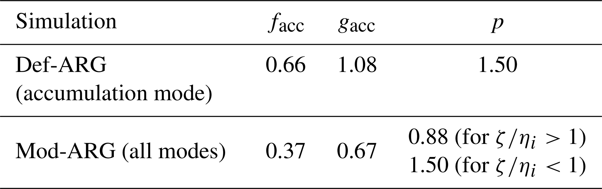
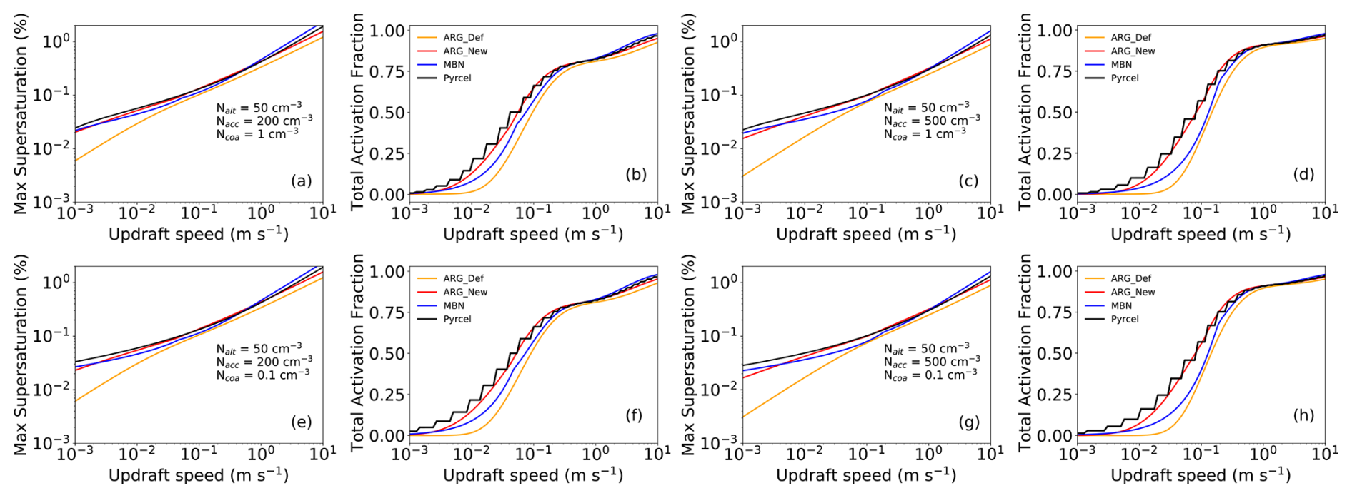
Figure 2 (a, c, e, g) show maximum supersaturation, while (b, d, f, h) show total activation fraction as a function of updraft speeds for the Pyrcel model, default ARG, modified ARG, and the Morales Betancourt and Nenes (2014) (MBN) schemes. Each pair (a, b; c, d; e, f; g, h) represents a different aerosol size distribution. The diameters of the Aitken, accumulation, and coarse mode aerosols are fixed at 40, 200, and 750 nm, respectively, with a hygroscopicity of 0.3 for all modes. The temperature is set at 283 K and pressure at 1 atm for all cases.

In Fig. 2, we compare the performance of the modified ARG scheme when run offline to Pyrcel simulations in conditions representative of fog, with updraft speeds ranging from 10⁻³–10⁻¹ m s⁻¹. We also compare the performance of the ARG parameterization with the Morales Betancourt and Nenes (2014) activation parameterization (hereafter MBN), which is more physically accurate but computationally expensive compared to the ARG scheme. We define the activation fraction as the number of droplets predicted by Pyrcel or the parameterization divided by the sum of the aerosol number concentrations in the Aitken, accumulation, and coarse modes. The Aitken mode here corresponds only to GLOMAP's Aitken soluble mode; the Aitken insoluble mode typically has higher aerosol concentrations within it, but these do not activate. The number concentrations of the accumulation and coarse aerosol modes are varied across the subfigures (the Aitken number concentrations are kept fixed) at 283 K temperature, and 1 atm pressure, representative values for ParisFog. In the parcel simulations, the geometric standard deviations correspond to those set in GLOMAP at 1.59, 1.4, and 2.0 for Aitken soluble, accumulation, and coarse aerosol modes. The hygroscopicity of all modes is fixed at 0.3. We find that the default ARG scheme (yellow lines) always significantly underestimates the activation fraction. The modified scheme (red lines) performs much better than the default ARG scheme and is often better than the MBN scheme.

For example, at updraft speeds between 0.01 and 0.1 m s⁻¹, the Pyrcel model usually activates 20 %–60 % aerosols, while the default ARG parameterization activates 0 %–50 %. In comparison, the updated ARG parameterization activates similar fractions to Pyrcel. In our UM simulations of fog, cases where the default scheme performs poorly (such as those in Fig. 2) occur frequently. Thus, in simulation Mod-ARG, we include our modifications to the ARG parameters (Table 3) to improve the performance of the ARG scheme. In Sect. 5, we show that this modification substantially improves the model's performance.

4.3 Modified ARG scheme with updated hygroscopicities (Mod-Kappa)

Aerosol activation in the model depends upon volume-weighted hygroscopicities for the aerosol modes, described using the κ–Köhler approach of Petters and Kreidenweis (2007). However, these numbers are not state-of-the-art in the standard configurations of the climate model (HadGEM3-GC3.1 and UKESM1) used in the most recent Coupled Model Intercomparison Project simulations (Mulcahy et al., 2020, 2023) nor in the NUMAC setup described by Gordon et al. (2023). By default, sulfate (and nitrate) is assumed to fully dissociate in solution, leading to a kappa value for sulfate, for example, of 0.97, while the kappa value of organic carbon is zero. A large corpus of literature provides convincing evidence (e.g., Petters and Kreidenweis, 2007; Schmale et al., 2018) that organic carbon is slightly hygroscopic, and that the hygroscopicity of sulfate aerosol is lower than 0.97, because it does not fully dissociate in solution.

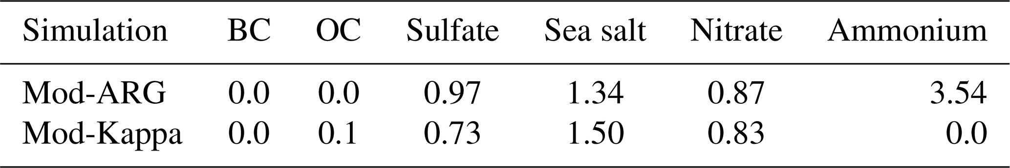
In this simulation (hereafter termed Mod-Kappa), we assign a κ of 0.1 to organic carbon (OC) (both primary and secondary organics), and, via an approximate approach, we arrive at kappa values close to the recommended 0.61 for ammonium sulfate and bisulfate, 0.73 for sulfuric acid (Schmale et al., 2018; Fanourgakis et al., 2019), and 0.67 for ammonium nitrate (Petters and Kreidenweis, 2007). This is achieved by setting the kappa values of the sulfate component in our model to 0.73, nitrate to 0.83, and ammonium to zero. This solution maintains the simplicity of having a single kappa value for each component species (e.g., sulfate) that does not vary according to which other species are present.

In Table 4, we list the hygroscopicities for different aerosol species used in Mod-ARG and Mod-Kappa. When we run our simulation with these new kappa values, we also include changes to the ARG scheme from the Mod-ARG simulation.

Table 4 Different values of hygroscopicities for different aerosol components used in the Mod-ARG and Mod-Kappa simulations. Nitrate and ammonium were not included in climate simulations for CMIP6.

5 Results

5.1 Location and timing of fog

We start our model evaluation by comparing the location of fog in the 4 km resolution model to satellite imagery. This evaluation demonstrates qualitatively how the model can simulate fog over a large domain with variable topography and some ocean, but the quantitative analysis in this paper focuses on the 500 m resolution model. Our satellite dataset is the fog product from the Spinning Enhanced Visible and Infrared Imager (SEVIRI) onboard the Meteosat Second Generation (MSG) satellites, operated by the European Organisation for the Exploitation of Meteorological Satellites (EUMETSAT) (Schmetz et al., 2002).

In Fig. 3, we show the location of the fog from simulation Def-ARG at 4 km resolution, on about half of the days during our case study period at 03:00 UTC. The satellite images (which correspond roughly to the 4 km resolution model domain) on the top panel show the location of fog in different colors depending on fog top temperature. For example, the simulated fog near the center of the domain is much thicker on 15 November than on 22 November. The SIRTA observatory is shown by a red dot near the center of the domain. At 03:00 UTC, we have some coverage of fog at the center of the domain on all days. On 15 and 16 November, the fog is much denser in the observations, but on 20, 22, and 23 November, the fog is patchy. The model could realistically simulate fog towards the English Channel and UK, although we underestimate marine fog on 16 and 23 November. Fog simulated in the top right corner towards Germany on 15 and 16 November is less widespread than satellite observations.

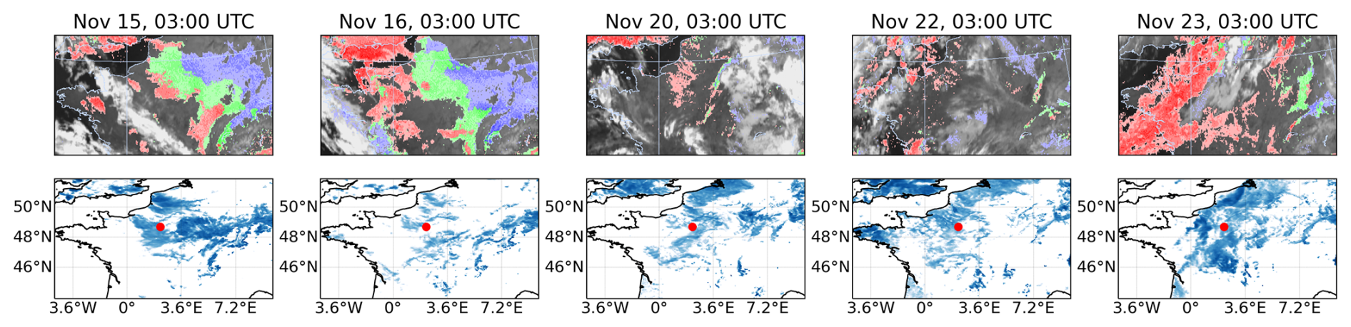
Figure 3 Location of the fog at 03:00 UTC during different representative fog events. The top panels show images from the Spinning Enhanced Visible and Infrared Imager (SEVIRI). Red refers to fog with fog top temperatures >1 °C, blue refers to fog top temperature $<-\mathrm{1}$ °C, and green refers to fog with fog top temperatures between 1 and −1 °C. The bottom panel shows the location of fog in the 4 km model. We show LWC (at the surface) across the domain in blue. Thicker fog is represented by a darker shade. The SIRTA observatory at the center of the domain is denoted by a red dot.

Overall, during our simulated period between 14 and 26 November 2011, 11 fog events were observed at SIRTA while, in our default simulation, 13 fog events were simulated in our 500 m-resolution domain. The onset of fog is usually well after dusk (21:00 to 03:00 UTC) on most days. The fog layer gradually develops and finally dissipates in the morning due to shortwave heating. When the fog top altitude is lower than 18 m, which is the case for the four observed events from 18 to 22 November, Mazoyer et al. (2019) characterized the fog as “thin”, while the seven other cases are thick fog.

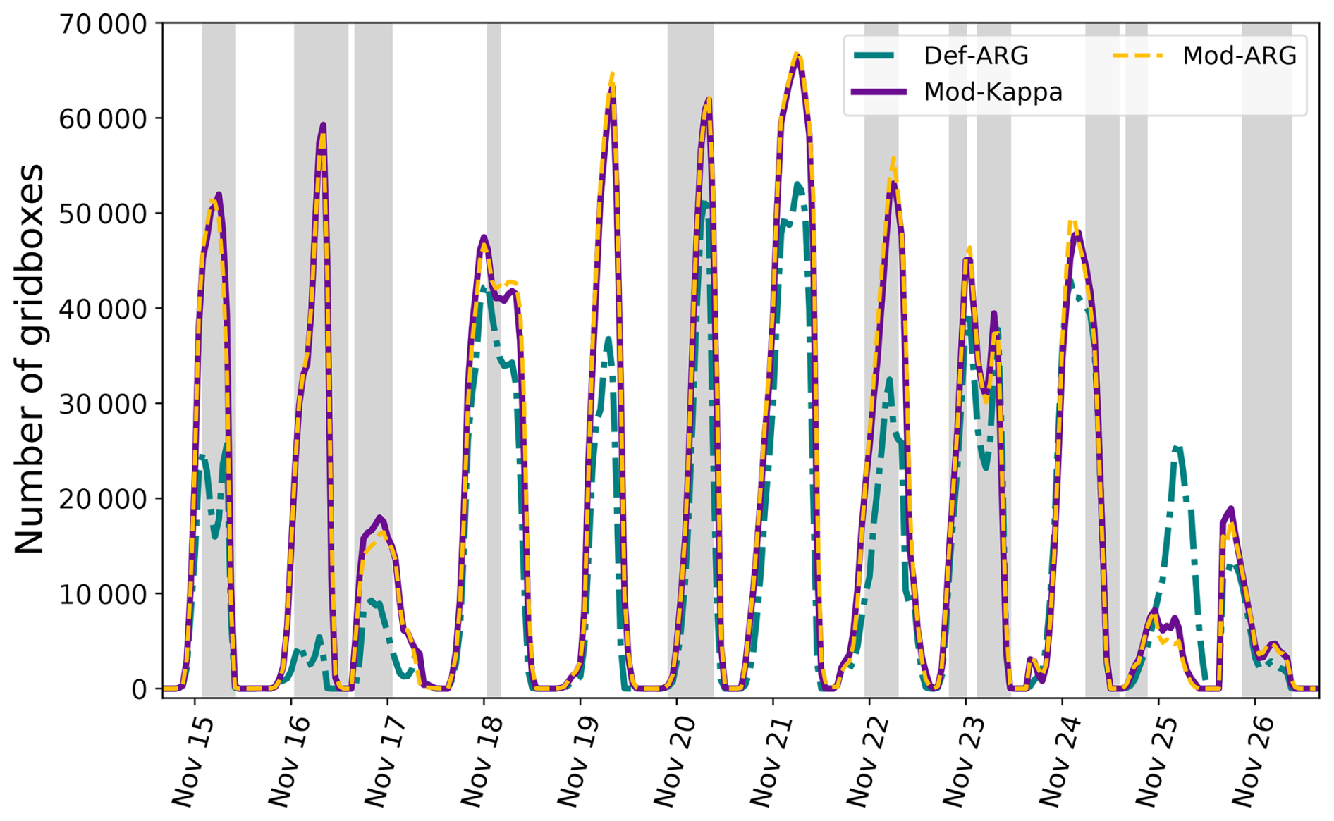
Figure 4 Time series of number of foggy grid boxes (at the surface) from the 500 m resolution model for simulations Def-ARG, Mod-ARG, and Mod-Kappa. If the entire domain was foggy, the total would be 67 600 (260×260). Foggy periods in the observations are shown in shaded gray. Tick marks on the x axis are at midnight UTC time.

Figure 4 shows a time series of the number of foggy grid boxes at the surface in the 500 m model from simulations Def-ARG, Mod-ARG, and Mod-Kappa. Mod-ARG and Mod-Kappa have nearly identical numbers of foggy grid boxes. The visibility parameterization of Gultepe et al. (2006) suggests that if N_d is 200 cm⁻³ and LWC is 0.005 g m⁻³, visibility would be ∼ 1 km. Therefore, we define foggy grid boxes as those having at least 0.005 g m⁻³ LWC (similar to Mazoyer et al., 2019) and at least 20 % cloud cover. Changing these thresholds by a factor of 2 does not make any significant difference. To avoid artifacts due to the interpolation of the grid from 4 km to 500 m resolution, we do not include the 20 grid boxes near the edges of the domain in the figure, regardless of the presence of fog. Therefore, the maximum number of foggy grid boxes at any given model level is 67 600 (260×260).

During the two weeks we simulated, the model produces a fog with a realistic lifetime for most of the fog events, however, the onset and dissipation times are not always correct (fog on the morning of 18 November starts too early, for example). On the mornings of 19, 21, and 25 November, the model predicts widespread fog but there was no fog in the observations at SIRTA. For the fog cases on 24 November, the timing of dissipation is either too early or too late across the simulations. For the second fog case on this day (Subfigure j), the Mod-Kappa simulation shows better agreement with observations up to 18:00 UTC, where Mod-ARG overestimates N_d by a factor of 2. Differences in droplet sedimentation velocity (discussed later) may have contributed to the variations in N_d. Some discrepancies are expected considering the difficulty involved in simulating fog accurately at the correct location using numerical weather prediction (NWP) models without data assimilation (e.g., Bergot et al., 2005; Zhou and Ferrier, 2008; Velde et al., 2010; Bergot, 2013; Steeneveld et al., 2015; Boutle et al., 2016, 2018; Martinet et al., 2020). However, we simulate enough fog to be able to examine aerosol effects on N_d and fog microphysics.

Differences in fog cover between Def-ARG and Mod-Kappa simulations arise via feedback mechanisms. For example, the higher modeled sedimentation velocity near the surface on 16 November in the Def-ARG simulation compared to the others leads to lower N_d and liquid water content, contributing to the reduced number of foggy grid boxes compared to Mod-ARG (as discussed later and shown in Figs. 14 and S14–S17). The differences are larger at the start of the simulation period, on 15 and 16 November, than towards the end. This may be due to the slightly higher altitude of the top of the inversion present during the first two fog events (next section) compared to most of the others. This higher inversion top could support enhanced feedback mechanisms (discussed later) that influence both N_d and fog top height. Exceptionally, on 24 November, the inversion top is also elevated, but the inversion does not start at the surface, and the fog onset is simulated much too early. In Fig. S1 in the Supplement we show the time series of average cloud fraction (at the surface) from the 500 m resolution model for simulations Def-ARG, Mod-ARG, and Mod-Kappa (only from the foggy grid boxes). The cloud fraction is consistently lower in Def-ARG compared to other simulations.

5.2 Evaluation of temperature and relative humidity profiles and time-series

We evaluate the ability of our model to simulate temperature and relative humidity (RH) realistically near the surface. Accurate representation of these parameters is important because too high temperature or too low relative humidity can lead to dissipation of fog, and fog often needs temperature inversions to form. Two radiosonde profiles are available each day at around 23:00 and 11:00 UTC. In Fig. 5, we compare the nighttime radiosonde profiles with our 500 m resolution Def-ARG simulation at the same location. Fog is not usually seen at the time of the daytime profile, but the profiles are available in Fig. S2.

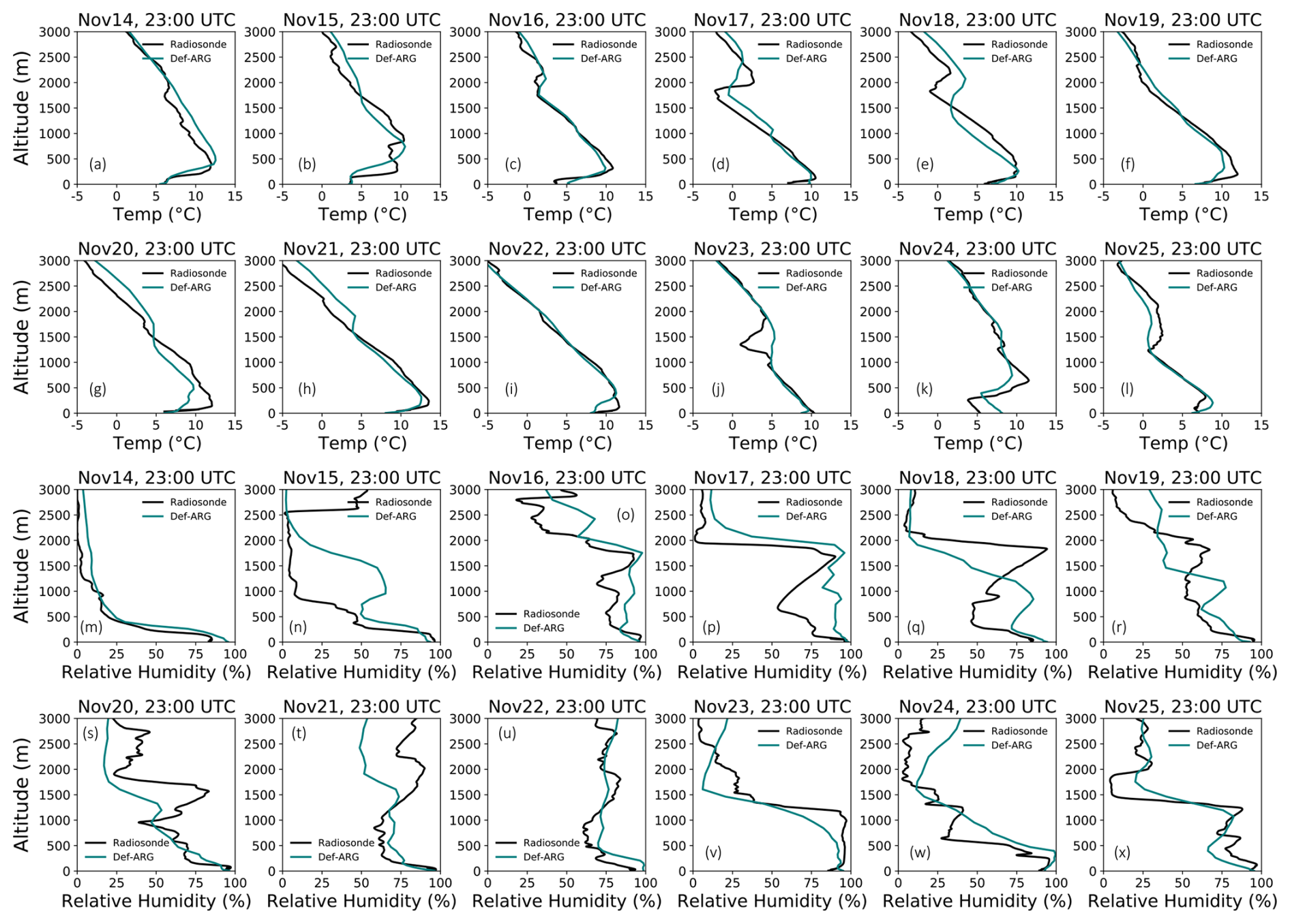
Figure 5 Vertical profiles of temperature and relative humidity from 500 m grid resolution model of simulation Def-ARG. The results are compared with the data from radiosondes launched from Trappes at around 23:00 UTC on 14 to 25 November.

Within 200 m of the surface at night, the simulated temperature profile in the 500 m domain is usually in reasonable agreement with observations, within 1 °C or so. Exceptions are on 20 November, where simulated temperatures above about 150 m altitude are approximately 2 °C too low, and the 24th when there is a ∼ 2.5 °C overestimation below 300 m altitude. Even a 0.5 °C bias may be enough to significantly affect the simulated fog. Nonetheless, the model can reproduce the surface inversion height and approximate strength on all days, except for 20 November when the inversion is too weak and 24 November when it is too high. The higher-level inversions were not always reproduced accurately. For example, on the 17th and 18th, the temperature profile above 1 km has biases of up to ∼3 °C.

Similar trends were observed for the RH profiles. Within 200 m of the surface, the 500 m model simulates RH realistically, within 10 % of the observation most of the time. RH near the surface has a larger positive bias on the 17th and a negative bias on the 25th. At a higher altitude, RH has much larger biases on most days. The model frequently fails to reproduce the detailed structure. In both simulations and observations, the fog top is usually near the surface, where the model performs best, but we must nonetheless consider that (especially) the radiative properties of the fog may be affected by biases in high cloud cover.

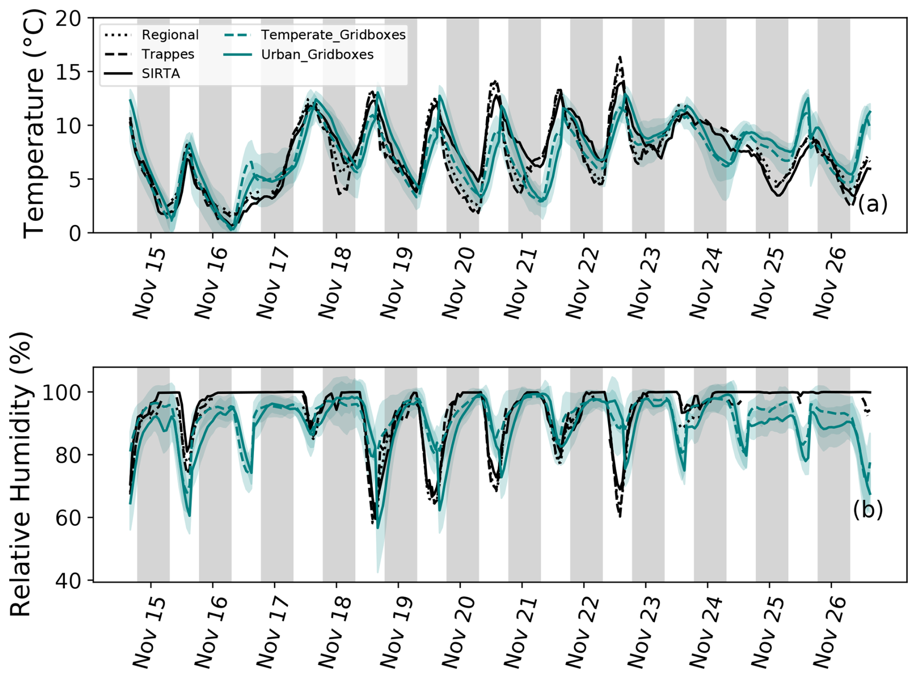
Figure 6 Observed and simulated near-surface temperature (a) and relative humidity (b) during different fog episodes. We show direct measurements from the sites at SIRTA and Trappes. “Regional” refers to weighted average temperature and RH calculated from measurements at Orly, Montsouris, and Trappes, following Sect. 3.2.1 of Chiriaco et al. (2018). The simulated “Temperate” and “Urban” time series are averages of all grid boxes denoted as “Temperate Grass” and “Urban”. The green shaded area shows the variability within ±2 standard deviations of the mean temperature and relative humidity.
Less frequently occurring surface types, such as water, are not shown here. Times are UTC and the gray shaded region denotes nighttime.

Figure 6 compares the observed temperature and RH time series with simulated temperatures (a) and RH (b) at “Temperate Grass” and “Urban” surface types. The green shaded area shows the variability within ±2 standard deviations of the mean temperature and relative humidity. We also show direct measurements from the sites at SIRTA and Trappes. We plot the regional weighted average using measurements from sites at Paris–Montsouris, Orly, and Trappes following Sect. 3.2.1 of Chiriaco et al. (2018). Nighttime is denoted by the gray shaded regions. Urban tiles are usually warmer and have lower RH than grass due to heat island effects. Features of the diurnal cycle, which are relevant to fog for both temperature and RH, are well simulated by the model.

For temperature, the R value of the time series is 0.80 and the normalized mean bias (NMB), defined as

$$\text{NMB}={\displaystyle \frac{{\sum }_i(M_i-O_i)}{{\sum }_i{O}_i}},$$

for simulated values M_i and observations O_i, is −0.08; for RH R is 0.49 and NMB −0.03. These statistics are calculated by comparing the mean profiles from four sites with mean profiles from model. There are missing data from observations on 17 and 24–26 November from one or more sites. The relatively low R value for the RH time series appears to be mostly due to an overestimation of RH by the model when RH is low (as on 22th), and when fog is not present. While observed RH usually falls within the modeled variability, substantial biases remain on certain days (e.g., 25 November). However, these RH biases are comparable to other numerical weather prediction simulations of these cases (Menut et al., 2014) and do not align consistently with errors in the onset or dissipation timing of fog. In contrast, temperature biases appear to be more influential – for example, on 21 November, the model underestimates the surface temperature, resulting in a false fog prediction at SIRTA. Moreover, at higher altitudes, the biases in temperature and RH can be much larger, leading to differences in cloud cover above the fog top.

5.3 Evaluation of aerosols

We investigate the ability of the model to simulate aerosols realistically in simulation Def-ARG. All simulations use the same set of boundary conditions and emissions inventory, so we do not expect the aerosol concentration to differ substantially between our simulations. Figure 7 demonstrates qualitatively how aerosols are simulated in our 4 km resolution model. Figure 7a shows the black carbon (BC) emission flux, to illustrate the major emission sources in our domain while using the high resolution EDGAR-HTAP inventory. BC particles contribute to number concentrations in the “Aitken insoluble” mode (Fig. 7b). Figure 7c shows the number concentration of accumulation “soluble” mode particles near the surface. We infer that CCN concentrations (which are mostly activated accumulation mode aerosols) are not obviously correlated with major emissions sources on this date.

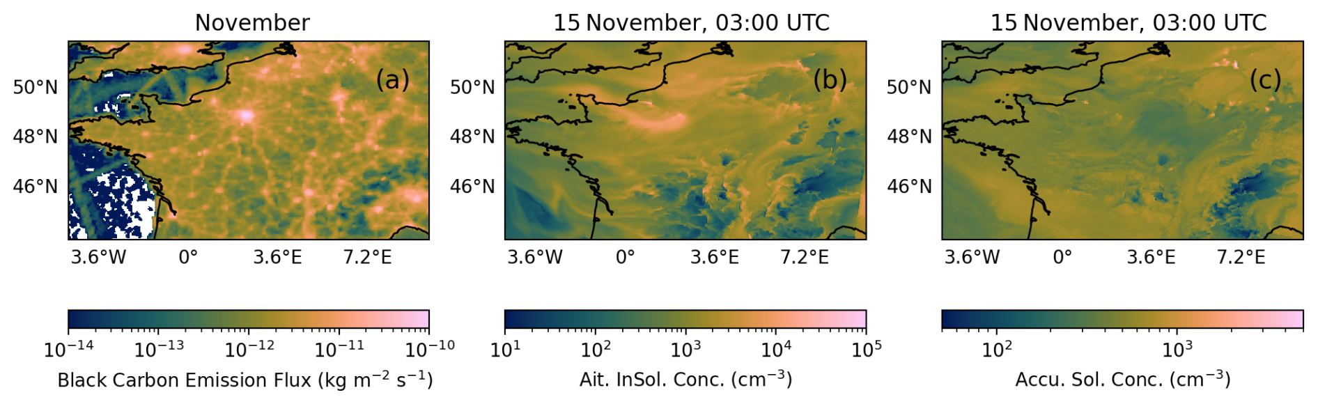
Figure 7 (a) shows the black carbon emission flux at the surface from the high resolution EDGAR-HTAP inventory in the 4 km model for the month of November. Hotspots such as London and Paris can be identified. (b) shows the Aitken insoluble mode number concentration and (c) shows the accumulation soluble mode particle number concentration, as simulated by the 4 km model in simulation Def-ARG near the surface at 03:00 UTC on 15 November.

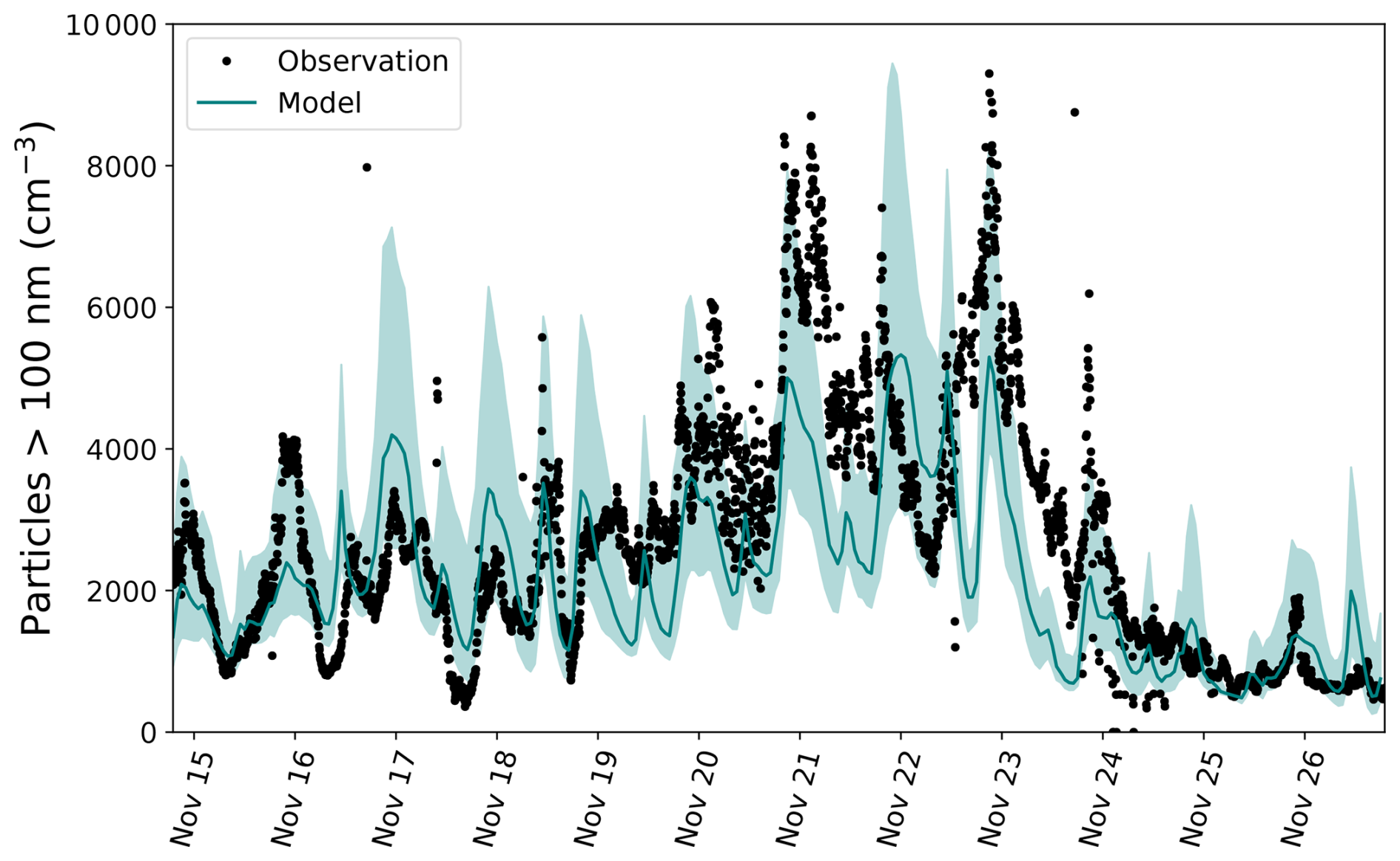
Figure 8 Time series of number concentration of aerosols greater than 100 nm in diameter as simulated by the 500 m model in the Def-ARG simulation at 5 m altitude, compared with the observations from SMPS in the same size range. The model median is represented by the green line and the shaded region represents the interquartile range. Times are UTC.

In Fig. 8, we compare the time series of simulated number concentration of >100 nm dry diameter aerosols with the near-surface observations from the SMPS at SIRTA. The simulated median number concentration from the 500 m resolution Def-ARG simulation is shown by a green solid line and the shaded region shows the interquartile range across the model domain. The region within 20 grid boxes of the boundary is excluded, as for our analysis of fog. As mentioned earlier, Fig. S3 shows time series of the number concentrations in the different GLOMAP lognormal aerosol modes. The simulated aerosol number concentration agrees reasonably well with the observations, with a correlation coefficient of 0.71 and a normalized mean bias of −0.18. These biases are typical, or better than typical, for simulated aerosol number concentrations in regional and global models (e.g., Baranizadeh et al., 2016; Williamson et al., 2019; Ranjithkumar et al., 2021).

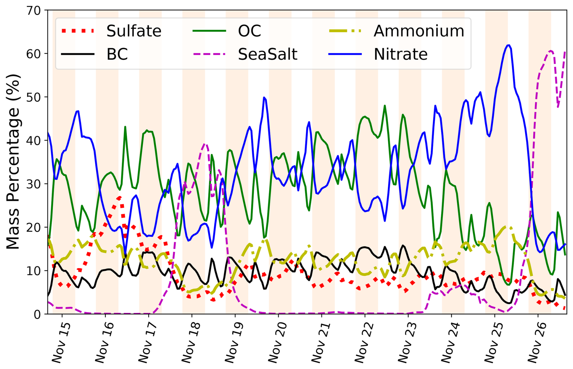
Figure 9 Percentage of different aerosol species by mass as a time series (UTC time) throughout the simulation period. The mean values from the grid boxes in the 500 m resolution Def-ARG simulation near the surface are shown. Nighttime is denoted by the shaded regions. All species the model represents with the GLOMAP microphysics scheme are shown; dust cannot participate in CCN activation.

In Fig. 9, we show the percentage of different aerosol species by mass as a function of time. Crippa et al. (2013) carried out a source apportionment study over Paris during winter in November with an aerosol mass spectrometer and Aethalometer. They found the following composition of aerosol by mass: 36 % organic carbon (OC), 28.4 % nitrate, 15.7 % sulfate, 11.9 % ammonium, 6.8 % black carbon (BC), and 1.2 % chloride. Another study in northern France in 2015–2016 (Roig Rodelas et al., 2019), found similar aerosol compositions. On average, our simulations have 28.2 % OC, 32.7 % nitrate, 9.2 % sulfate, 12.3 % ammonium, 9.4 % BC, and 8.2 % sea salt (4.9 % chloride) aerosol mass (see Table 5). Hence, most likely our simulations are realistic, but they probably underestimate organic aerosols. Secondary organic aerosol (SOA) formation from anthropogenic volatile organic compounds and isoprene is not included in our model and could explain the bias. Since aerosol number concentrations align well with observations and N_d is relatively insensitive to hygroscopicities (as demonstrated later), the relative underestimation of sulfate and organic aerosols is unlikely to significantly impact N_d.

Crippa et al. (2013)

Table 5 Percentage composition of aerosols over Paris from Crippa et al. (2013) and the 500 m model (simulation Def-ARG, at the surface) is listed here.

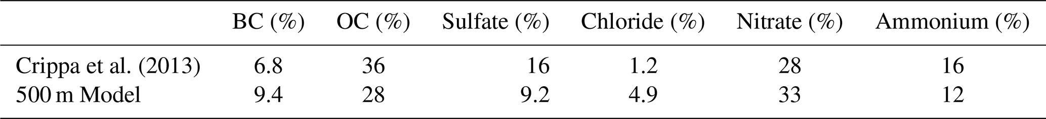
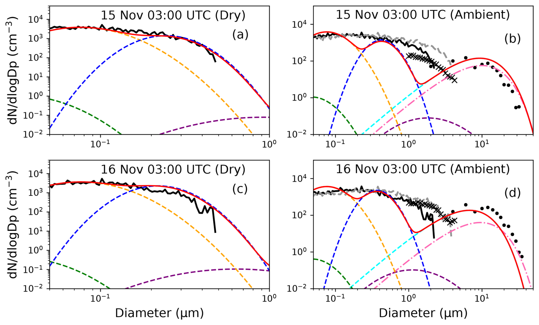
Figure 10 Dry and ambient aerosol size distribution on 15 and 16 November at 03:00 UTC from observations and our Mod-Kappa simulation. Only foggy grid cells are shown. The dry size distribution is measured by the SMPS only, while the WELAS and fog monitor (FM) observed the size distribution at ambient relative humidity. For this ambient size distribution, we also converted dry particle concentration data from the SMPS to ambient using κ–Köhler theory assuming a kappa value of 0.1 (and 0.3) and 100 % relative humidity. The red line shows simulated total dry and ambient humidity particle size distributions, while the dashed lines show the different aerosol and droplet modes. The dashed pink line shows N_d from simulation Def-ARG.

Figure 10 shows the aerosol dry and ambient or hydrated size distributions from our 500 m Mod-Kappa simulation, compared to observations at 03:00 UTC on 15 and 16 November. The solid red line represents the total number of particles (and also N_d for the ambient humidity size distribution subfigure) simulated by the model. Through the dashed pink line, we show the N_d distribution from Def-ARG simulation. Similar plots at the same time on 18, 20, 22, and 26 November are shown in Fig. S4.

On the days shown in Figs. 10 and S4, the model overpredicts the aerosol concentrations in the Aitken insoluble mode. The aerosol size distributions are in better agreement for the accumulation mode, except on the 20th where it is underestimated. The ambient humidity size distributions show that a more substantial underestimate of the number concentrations is usually observed in the coarse mode (0.01–1 cm⁻³). This seems to be the main symptom of the inability of the aerosol microphysics scheme to accurately simulate haze, discussed earlier.

On 15 November, N_d in the default simulation agrees well with the observations, but on the other three days N_d is severely underestimated. However, a significant improvement is observed in Mod-Kappa, which we show in later figures is due to the change between Def-ARG and Mod-ARG. Also, so far, the difficulties in simulating haze do not appear to prevent a good simulation of droplet concentrations. The next sections investigate in greater detail the model performance in simulating fog droplets.

5.4 Evaluation of fog droplet concentration and liquid water content

The 500 m grid resolution simulations show widespread but inhomogeneous fog LWC and N_d during most fog events. To illustrate spatial variability, example patterns are shown from the Def-ARG simulation three times during the fog event on 15 November in Fig. 11 at 5 m altitude. The domain is foggy at late night and early in the morning and dissipates around 09:00 UTC. Similar figures during four other fog events are shown in Figs. S5–S8.

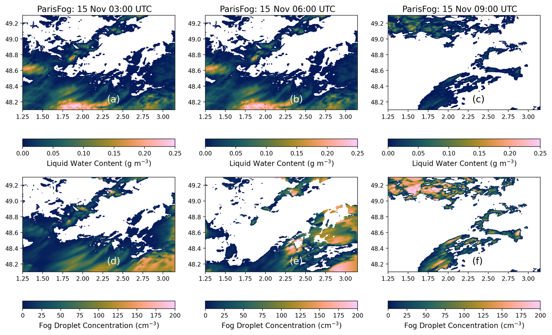
Figure 11 Spatial distribution of LWC (a–c) and N_d (d–f) near the surface (5 m altitude) at different UTC times on 15 November from simulation Def-ARG. These results are from the 500 m resolution model. The criteria for identifying a grid box as foggy are explained in Sect. 5.1 and Table 6; grid cells that do not meet the criteria are white.

In Fig. 12, we plot the time series of in-fog N_d for different fog events from our 500 m model, compared to observations from the fog monitor at SIRTA. In each grid box, in-fog N_d is calculated by dividing the grid-averaged N_d by the fractional cloud cover. To allow a comparison even when simulated and observed fogs are not exactly co-located as in Fig. 11, we show the medians as solid (and dashed) lines and the interquartile ranges over all of the foggy grid boxes as shaded regions. We also impose a minimum threshold of 1000 foggy grid boxes while calculating the domain median and IQR, as shown in Table 6. This threshold corresponds to about 1.5 % of the area of the entire domain and is designed to eliminate cases where fog forms only in isolated locations that are unlikely to be representative of the SIRTA observatory.

Table 6 Summary of different thresholds used to prepare N_d and LWC time series plots. Min_Fog denotes the threshold number of foggy grid boxes, below which a spatial average of the model domain for a time series is not calculated. n/a: not applicable.

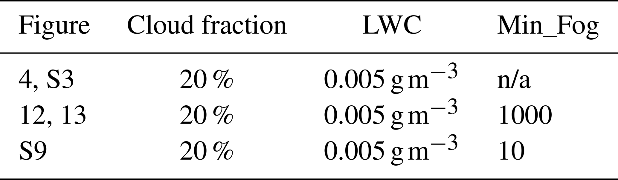
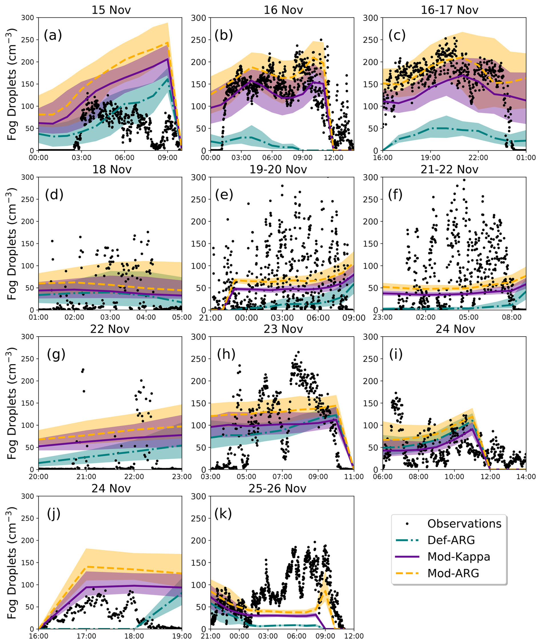
Figure 12 Variation of simulated and observed N_d as a function of time for different fog events. 500 m model results at 5 m altitude from simulations Def-ARG, Mod-ARG, and Mod-Kappa are compared with observations at the SIRTA observatory (UTC time). Different lines represent the median value and shaded regions represent the interquartile range over the foggy grid boxes. Figure S11 shows that including a contribution from sub-grid scale updraft velocities in the activation scheme has a similar effect as changing from Def-ARG to Mod-ARG, and that with higher updraft speeds the effect of the change from Def-ARG to Mod-ARG on N_d would often be much smaller.

Simulation Def-ARG was designed to understand the performance of the “ARG” activation scheme as implemented in the CASIM microphysics code in simulating N_d in fog. The observed N_d mostly varies between 0–300 cm⁻³ among different fog events. We calculate the normalized mean bias factor (NMBF) and the normalized mean error factor (NMEF), defined as

$$\begin{array}{ll}{\displaystyle }\text{NMBF}(\stackrel{\mathrm{‾}}{M}\ge \stackrel{\mathrm{‾}}{O})& {\displaystyle }={\displaystyle \frac{{\sum }_i(M_i-O_i)}{{\sum }_i{O}_i}}\\ {\displaystyle }\text{NMBF}(\stackrel{\mathrm{‾}}{M}<\stackrel{\mathrm{‾}}{O})& {\displaystyle }={\displaystyle \frac{{\sum }_i(M_i-O_i)}{{\sum }_i{M}_i}}\\ {\displaystyle }\text{NMEF}(\stackrel{\mathrm{‾}}{M}\ge \stackrel{\mathrm{‾}}{O})& {\displaystyle }={\displaystyle \frac{{\sum }_i|M_i-O_i|}{{\sum }_i{O}_i}}\\ {\displaystyle }\text{NMEF}(\stackrel{\mathrm{‾}}{M}<\stackrel{\mathrm{‾}}{O})& {\displaystyle }={\displaystyle \frac{{\sum }_i|M_i-O_i|}{{\sum }_i{M}_i}}.\end{array}$$

Here, M_i is the model data, O_i is the observation data, $\stackrel{\mathrm{‾}}{M}$ is the model mean, and $\stackrel{\mathrm{‾}}{O}$ is the observation mean. NMBF has a range of −∞ to +∞ and NMEF has a range of 0 to +∞. We report NMBF and NMEF for all fog cases in Tables S1 and S2 in the Supplement and use them as a tool to compare the model performance among different simulations.

By comparing the median time series shown by the dashed green line, for some of the fog cases, the default simulation is in satisfactory agreement with the observations, such as the fog cases on 15 and 24 November early in the morning (Fig. 12a and i). For these cases, we find NMBF values of 0.74 and 0.06, and NMEF values of 1.02 and 0.71. However, most of the time, the simulation Def-ARG severely underpredicts N_d. For example, in both fog events on the 16th, and in cases on the 21th and 25th (Fig. 12b, c, f, and k), the simulated droplet concentrations are lower than observations by more than a factor of 4 (NMBFs equal to −9.01, −3.31, −7.08 and −4.09). However, the severe underestimation on 20 November could be attributed to a negative bias in aerosol concentrations in the accumulation mode (by about a factor of 2, as shown in Fig. S4d) and somewhat large temperature biases (2–3 °C). Aerosol concentrations are also somewhat underestimated for fog cases between 19 and 23 November, which may have contributed to the lower simulated values of N_d. Figure S9 shows the time series of droplet concentrations during fog events from only foggy grid boxes within a 20×20 cell box around SIRTA. Selecting only these grid boxes does not change the significant underestimate of N_d on average.

In the Mod-ARG simulation, we introduced improved parameters for the ARG scheme (Ghosh et al., 2025a). In the Mod-Kappa simulation, we adjusted the hygroscopicities to more realistic values, reducing that of sulfate while increasing it for organic aerosols. As expected from the activation parameterization tests shown in Fig. 2, in simulation Mod-ARG N_d usually increases significantly compared to Def-ARG. Model performance is improved in most fog events. During the two thick fog events on the 16th (subfigures b, c), NMBF (NMEF) changed from −9.01, −3.31 (9.25, 3.45) in Def-ARG to 0.23, 0.25 (0.38, 0.31) in Mod-ARG. Similar performance improvements are also observed on 19 and 21 November fog cases. The NMBF (NMEF) improves from −5.18, −7.08 (5.83, 8.07) to −0.41, −0.19 (1.00, 0.85). In the 18th and 24th (morning) fog cases (subfigure d, i), the performance between default and updated simulations is very similar. On 26 November, the factor of 10 underestimation after midnight is now within a factor of 3. Overall NMBF (NMEF) changes from −4.09 (4.46) to −0.69 (1.02). On this day, the fog dissipation is better simulated in Mod-ARG compared to Def-ARG. For the 22 November evening fog event (Subfigure g), on average the default simulation is better, but relatively higher N_d between 22:00 and 23:00 UTC is slightly better simulated in Mod-ARG. On 24 November evening (subfigure j), the default simulation fails to produce fog most of the time, while good agreement of N_d is simulated with our improvements during fog formation and growth. In both simulations, the dissipation of fog is not accurate in the model. On 15 November, N_d is overestimated (NMBF increases to 2.69 from 0.74 in the default simulation) as a result of our changes; however, the overestimation is slightly higher than a factor of 2.

N_d decreases across all fog cases in Mod-Kappa (yellow in Fig. 12), mainly due to the lower hygroscopicity of sulfate aerosols. However, the change in N_d from Mod-ARG to Mod-Kappa is smaller than that of Def-ARG to Mod-ARG. Our findings align with Mazoyer et al. (2019), which found no significant correlation between N_d and κ in the ParisFog cases we study. In the model, for most fog cases, Mod-Kappa further improves model performance over Mod-ARG. On 15 November, the NMBF decreases from 2.69 to 1.97. For the 16 November cases, N_d remains in good agreement with observations. Similarly, on 24 November, the NMBF drops from 0.27 and 3.28 to −0.17 and 2.05. However, for fog cases on 19–20, 21–22, and 26 November (subfigures e, f, k), the reduction in droplet concentrations leads to degraded model performance compared to Mod-ARG. NMBF (NMEF) changes from −0.41, −0.19, −0.69 (1.00, 1.00, 1.01) in Mod-ARG to −0.96, −0.64, −1.52 (1.42, 1.24, 1.78). Nonetheless, the model is still in much better agreement with the observations compared to Def-ARG.

We expect that the underestimate in N_d in Def-ARG is caused by an underprediction of the fraction of aerosols activated at low updraft speeds by the default ARG parameterization, and by an underestimation of the updraft speed in the activation scheme that results from not resolving all the turbulence. Figure S10 shows the diagnosed unresolved sub-grid vertical velocity standard deviations in our simulations (subfigures c and f). Qualitatively, the values seem likely to be realistic if compared with the turbulent kinetic energy (TKE) shown in ParisFog observations by Stolaki et al. (2015) on 15 November, though the comparison is imprecise since TKE contains horizontal contributions, and some vertical velocity variance is resolved by our model and therefore not included in the sub-grid component.

In Fig. S11, we show two simulations in which the updraft speeds in Def-ARG and Mod-ARG are increased by including a component to represent sub-grid-scale, unresolved vertical turbulence. This turbulence component includes an ad-hoc tuning factor of 0.2 to keep N_d realistic; as mentioned earlier, dedicated future studies are needed to fully explore the turbulence contribution. Figure S11 confirms that the underestimation of N_d in Def-ARG could be largely resolved either by using Mod-ARG parameters or by adding a sub-grid component of updraft speeds with a tuning factor. Including both modifications leads to an overestimate of N_d, with NMB positive for all fog events and above 1.0 (a factor 2 overestimate) in 6 out of 11. In the companion paper, we will explore strategies to mitigate the overestimations of N_d, which may also be beneficial when the impacts of sub-grid turbulence are more fully addressed in the future. Furthermore, Fig. S11 shows that the differences in N_d between Def-ARG and Mod-ARG in Fig. 12 would be substantially smaller if we included a subgrid turbulence contribution to updrafts for aerosol activation, a result that could also be inferred from Fig. 2.

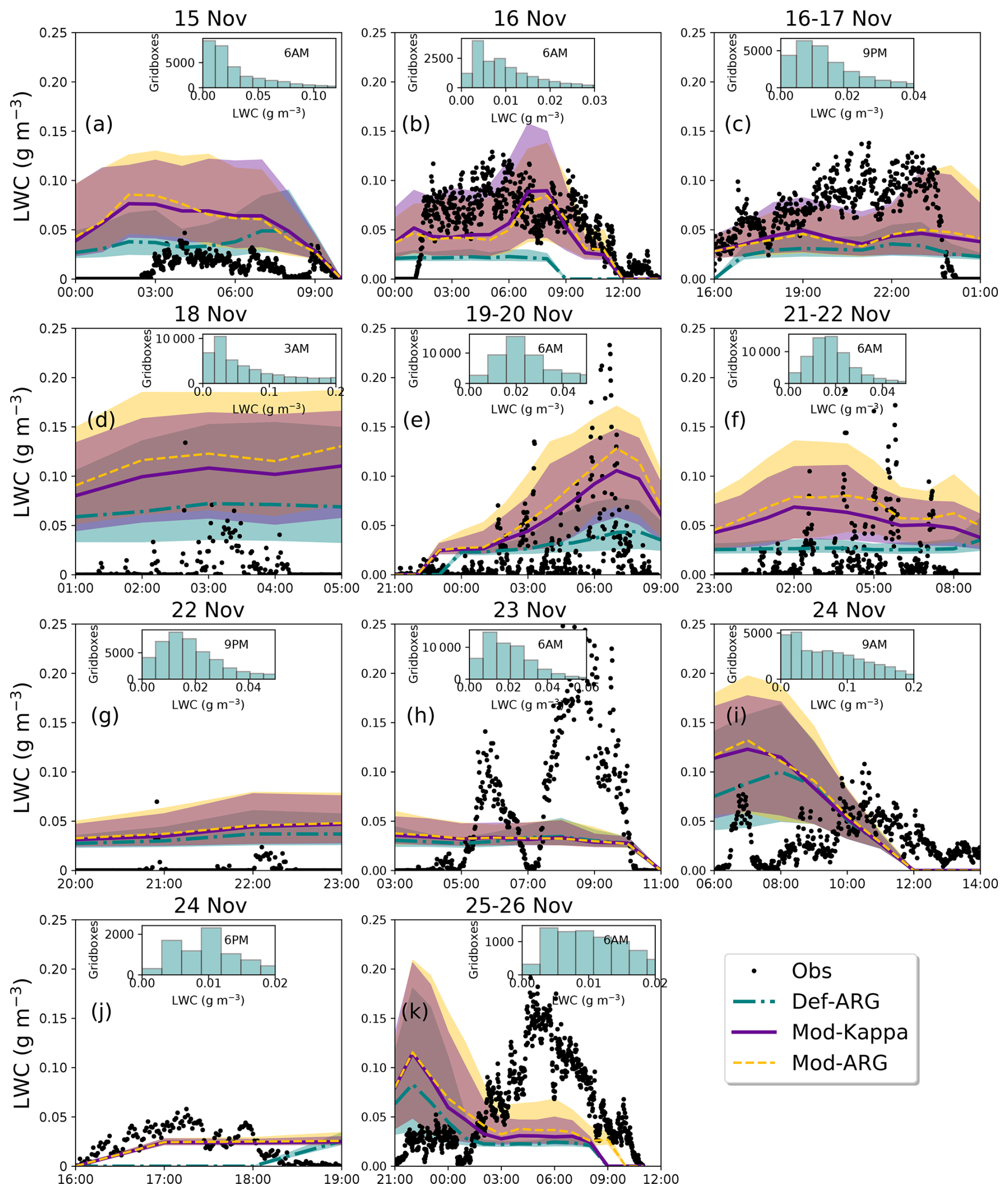
Figure 13 Variation of LWC as a function of time (UTC) for different fog events in the 500 m resolution regional model. (a–k) compare all the simulations with the observations for the different fog cases. The solid lines and shaded regions represent the median and interquartile range from foggy grid boxes. The inset plots show histogram of in-fog liquid water content at different times of the fog events. The minimum LWC visible in the plots of around 0.025 g m⁻³ is due to the thresholds for defining grid boxes as foggy, as described in the text.

In Fig. 13, we compare the time series of in-fog LWC in foggy grid boxes to observations. Figure 13a–k shows different fog cases. In-fog LWC is calculated by dividing the grid average LWC by the cloud cover and the same grid box number threshold as in previous figures is applied. As shown in Fig. 4, most of the time the model simulated enough foggy grid boxes in the domain during all the events for the statistical properties (median and interquartile range) to be meaningful. At other times, the LWC is zero. When there are sufficient foggy grid boxes, the LWC and cloud fraction thresholds for defining these grid boxes as foggy leads to a minimum in the LWC of around 0.025 g m⁻³. Since low LWC grid boxes also tend to have low cloud fraction, the minimum here is the LWC threshold of 0.005 g m⁻³ divided by the cloud fraction threshold of 20 %. The interquartile ranges shaded on the time series in Fig. 13 show the general nature of the variability between grid boxes, while the inset figures on each subplot are histograms of in-fog LWC that give more detail at a particular time of the corresponding fog event, from the default simulation. In all fog events irrespective of thickness and type, there is substantial spatial variability of the simulated LWC in the 500 m resolution model as shown in the inset histograms. Therefore the observations at the SIRTA observatory may be quite different from the domain averages we present from the model. Figure S12 shows only the 20×20 grid boxes around SIRTA; however, the general trends in LWC in this figure do not look much different to Fig. 13.

While our simulations are mostly able to produce fog at the right time and despite reasonable simulations of N_d, neither Def-ARG nor Mod-ARG simulations have much skill in representing LWC on many of the days. Visually, trends in the time series only roughly match observations during three fog events of 11 (the two events on the 16th and the event on the 24th). This low skill may be partly an artifact of comparing a point observation with a domain average (Schutgens et al., 2017). Low skill is also expected from recent intercomparison studies (Boutle et al., 2022), in which LES and single column models were also found to have little skill in simulating liquid water path, even for a case our model is able to simulate reasonably well (see Fig. S13 and the companion paper). Realistic simulations of surface N_d, perhaps within 50 % of observations, may (or may not) be a necessary condition, but are clearly not a sufficient condition, for realistic simulations of LWC. Similarly to the N_d time series, LWC is underestimated during several fog events in simulation Def-ARG, such as for fog cases on 16 and 23 November, around 04:00–06:00 UTC on 21 and 24 November, and after fog onset on 25 November. During these periods, the bias is larger than a factor of 5. LWC in the observations is mostly between 0−0.20 g m⁻³, but LWC in the default simulation is always <0.10 g m⁻³. However, on some days, such as 15 and 20 November (on average), the default model performance was satisfactory (within a factor of 2 bias). Simulation Def-ARG (and other simulations as well) did not reproduce the thick fog on 23 November. The LWC time series could be affected by errors in the simulated higher-level cloud properties on this day. The model simulates substantial cloud cover above 300 m altitude, and the temperature and RH profiles between 500 and 3000 m altitude (Fig. 5) have errors of up to 3 °C and 15 % respectively, suggesting that these clouds may not be realistic. In addition, simulated aerosol concentrations were much lower than observations (Fig. 8).

Similar to N_d, there is a large difference in LWC between Def-ARG and Mod-ARG, and smaller differences between Mod-ARG and Mod-Kappa. The large difference between Def-ARG and Mod-ARG suggests that aerosol–fog interactions are important, at least in our simulations. Changes in the ARG scheme, increasing N_d, result in a significant increase in LWC compared to the default simulation. However, compared to the observations, it is unclear whether biases increase or reduce with this change. The most obvious mechanism that could explain the sensitivity of the simulated LWC to N_d in these simulations is the size dependence of droplet sedimentation rates. Figures 10 and S4 show that the droplets in Def-ARG are, on average, around 3–10 µm larger than in Mod-ARG, at least at the particular times we show.

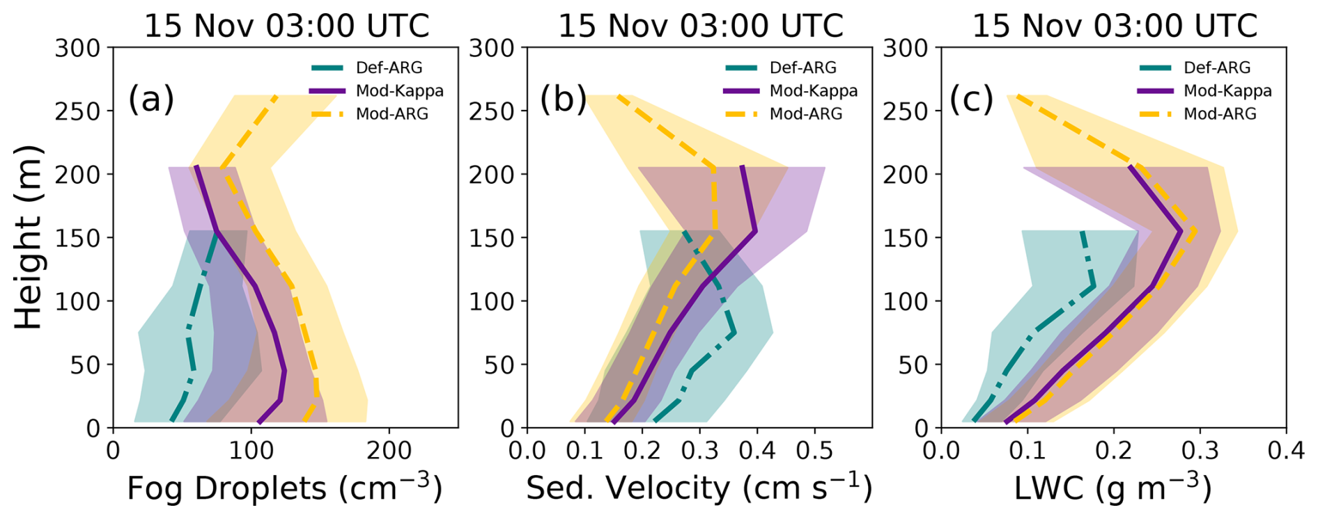
Figure 14 Vertical profiles of N_d (a), droplet sedimentation velocity (b), and LWC (c) in fog for the 15 November ParisFog case (at 03:00 UTC) for different simulations.

In Fig. 14, from the 500 m model, we show simulated vertical profiles of N_d, LWC, and sedimentation velocity at 03:00 UTC for the 15 November fog case. The increase in LWC from Def-ARG to Mod-ARG and Mod-Kappa in this case is fairly typical for this increase in N_d; profiles from some other fog cases shown in Figs. S14–S16 are discussed in more detail in the companion paper. Where there is substantial fog, Def-ARG has higher sedimentation rates. However, other aerosol–cloud interactions mediated by radiation are also possible. For most fog cases, a higher LWC in Mod-ARG also leads to a higher fog top height, perhaps due to increased turbulence (also see Fig. S17). A positive feedback mechanism can be proposed as follows: (a) reduced droplet sedimentation increases the liquid water path, enhancing cloud-top radiative cooling. Radiative cooling may also be increased directly due to the smaller droplet effective radius, which leads to more efficient absorption of upwelling surface radiation that is subsequently re-emitted (Boutle et al., 2018). (b) Enhanced radiative cooling promotes further condensation of water vapor and intensifies turbulence (Boutle et al., 2018), resulting in a much optically thicker fog layer. (c) The increased turbulence then accelerates condensation through adiabatic cooling, raising the liquid water path and lifting the fog top, both of which contribute to even greater radiative cooling rates. On 15 and 16 November, the fog coverage in Def-ARG is much lower compared to other simulations, as discussed earlier. However, on 16 November, the inversion height is slightly higher than on 15 November, allowing these proposed feedback mechanisms to develop further. Furthermore, the droplet sedimentation velocity in the Def-ARG simulation on 16 November is higher (0.3 cms⁻¹) compared to 15 November (0.1 cms⁻¹), resulting in a larger sink of droplets. Hence, we find that on 16 November, the difference in fog top height between simulations is much larger compared to 15 November, and the default simulation severely underestimates the droplets on the 16 November case. While these processes are very likely interrelated, this feedback mechanism remains speculative. More detailed models with finer grid resolution might more accurately represent possible counterbalancing effects, for example, enhanced evaporation in the entrainment zone when sedimentation rates are reduced (Bretherton et al., 2007).

5.5 Evaluation of fog top droplet concentrations

In Fig. 15, we compare simulated droplet concentrations at the top of the fog to retrievals from the Moderate Resolution Imaging Spectroradiometer (MODIS) Terra satellite. The satellite retrievals have large uncertainties, but they do allow us to evaluate (to some extent) the spatial variability of the droplet concentration across our model domain, which the SIRTA measurements do not.

We calculated N_d using observations of cloud optical depth, cloud droplet effective radius, and cloud top temperature from MODIS, using the Collection 6 Level 2 dataset, and following equations 1–11 described by Grosvenor et al. (2018). These equations assume that the vertical profile of liquid water content is adiabatic, which is clearly erroneous in some of the fog cases (the vertical profiles of LWC and N_d from a few ParisFog cases are shown in Figs. S11 and S13), but perhaps better than any other possible simple assumption. The fog top droplet concentrations can be calculated as

$$\begin{array}{}\text{(4)}& N_{\mathrm{d}}={\displaystyle \frac{\sqrt{\mathrm{5}}}{\mathrm{2}\mathit{\pi }k}}{\left({\displaystyle \frac{f_{\text{ad}}{c}_{\mathrm{w}}{\mathit{\tau }}_{\mathrm{c}}}{Q_{\text{ext}}{\mathit{\rho }}_{\mathrm{w}}{r}_{\mathrm{e}}^{\mathrm{5}}}}\right)}^{\frac{\mathrm{1}}{\mathrm{2}}}.\end{array}$$

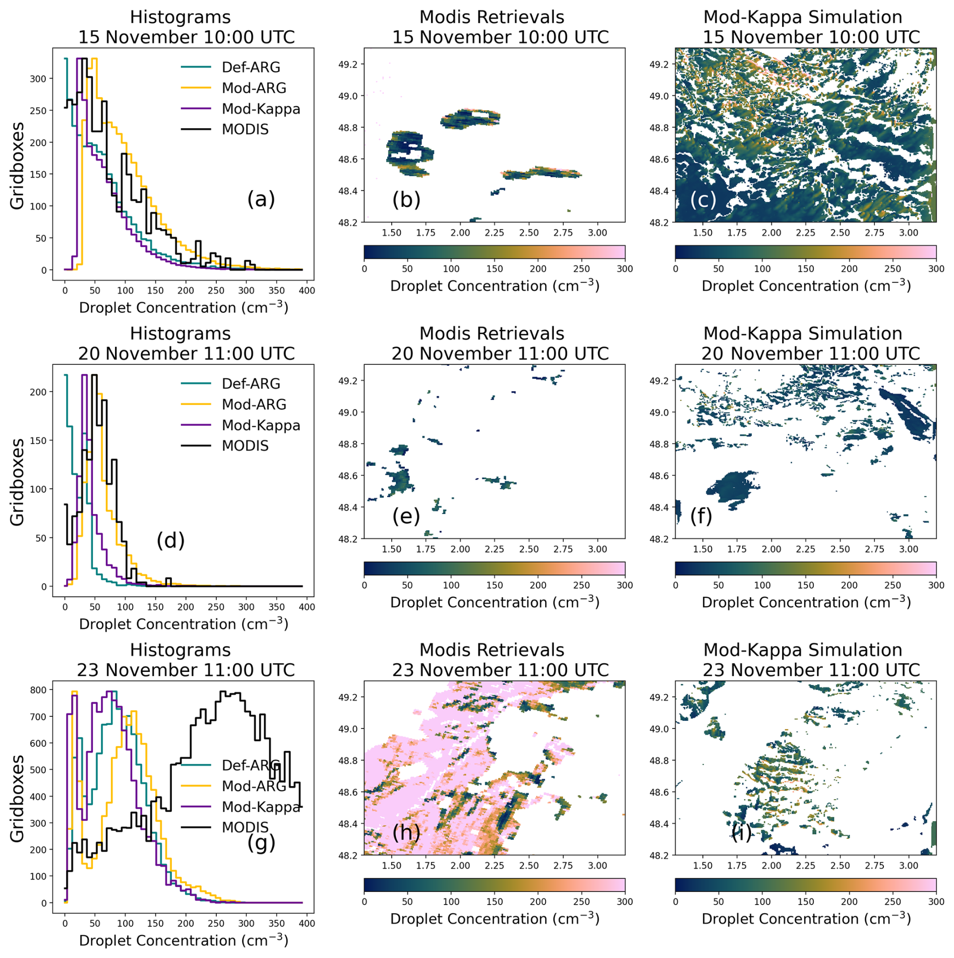
Figure 15 Histogram of fog-top N_d from Def-ARG, Mod-ARG and Mod-Kappa compared with N_d observations from MODIS satellite (a, d, g). Spatial variation of N_d from MODIS in the 500 m model domain is shown in (b, e, h). The spatial variation of N_d from the Mod-Kappa simulation in the 500 m model for different ParisFog cases is presented in (c, f, i).

The constant k is the ratio of the volume mean droplet radius to the effective radius, while f_ad is the degree of adiabaticity. We use k=0.8 and f_ad=0.7 following Grosvenor and Wood (2014). c_w is the rate of increase in liquid water content with height for a moist adiabatic ascent. τ_c is the cloud optical thickness. Q_ext is the extinction efficiency factor, set to 2 following Hulst and van de Hulst (1981). ρ_w is the density of water.

We show the spatial variation of fog top droplet concentrations in the 500 m model from the MODIS satellite (subfigures b, e, h) and the MOD-Kappa simulation (subfigures c, f, i) for the ParisFog cases on 15 November 10:00 UTC, and on 20 November and 23th at 11:00 UTC. We show MODIS data only for those locations where the cloud top height is below 1.5 km; higher cloud is the primary reason why subfigures b and e appear sparse. We also show the histogram of N_d from the Def-ARG, Mod-ARG, and Mod-Kappa simulations and compare them with the MODIS-derived droplet distribution (subfigures a, d, g). We normalized the histograms to account for different numbers of foggy/cloudy grid boxes in different simulations. The selected days are the only days on which MODIS sees significant cloud with top height below 1500 m. Unfortunately, on 23 November, our evaluation at SIRTA showed that fog LWC is very poorly simulated by the model, so we do not expect good results. On the other two days, we have fewer valid retrievals, but still hundreds to thousands in total, enough to gain some insight into the N_d variability.

Similar to the fog monitor measurements presented earlier, we find that the default simulation severely underestimates N_d. With updates to the ARG scheme (and hygroscopicity fixes) in simulation Mod-Kappa, the N_d distributions are in much better agreement with the observations (considering only 15 and 20 November). Both the mean and spatial variability appear to match reasonably well.

We find that the spatial variability in N_d is simulated realistically on both 15 and 20 November. However, we also find that the spatial variability at cloud-top does not match the temporal variability at the surface (for example, the spatial standard deviation of cloud-top N_d on 15 November from MODIS is 99 cm⁻³ while the temporal standard deviation during the same fog event from the fog monitor is 38 cm⁻³ at the surface). Therefore, the shaded ranges representing spatial variability we show on Figs. 12 and 13 are only approximately comparable with the temporal variability in the observations. While the comparison of simulation and satellite data is valuable because it gives a sense of real observed spatial variability in N_d, the evaluation of simulated N_d with MODIS-derived N_d must be interpreted with care. Firstly, the satellite measurements have large uncertainties, estimated at 78 % at the pixel level by Grosvenor et al. (2018) even for relatively adiabatic clouds. Additionally, we cannot be sure our MODIS retrievals are of fog rather than cloud. The retrieved cloud top height used in both our 1.5 km threshold for “likely fog” and in the N_d retrieval itself is uncertain, and layers of cloud that is not fog may still have tops below 1.5 km. Indeed, we know that many of the fogs we study are obscured by higher cloud (although this is often simulated poorly by the UM). However, the contrasting results near the surface and at the fog top, combined with uncertainties in satellite retrievals, further motivate the need to study the vertical structure of fog using ground-based observations – an effort addressed in the companion paper.

6 Discussions and conclusions

The activation of fog droplets at the SIRTA observatory near Paris is studied with a weather and climate model. The aim is to examine how well aerosol and cloud microphysics designed for (relatively) computationally inexpensive weather and climate simulations can simulate droplet concentrations in fog. We simulated 11 fog events that were observed during the 2011 ParisFog field campaign, using a 500 m resolution setup. The aerosol microphysics scheme simulates reasonably realistic aerosol number concentrations and size distributions, and the nitrate aerosol scheme of Jones et al. (2021), tested here at kilometer-scale spatial resolution for the first time, also seems to perform well. The key findings of our work are listed below:

• The model produces satisfactory simulations of fog cover, given that forecasting fog is difficult: the model could produce some fog in our 500 m domain during all fog events observed at SIRTA, but the fog was not always co-located with the observations and there were some simulated fogs that did not correspond to observations.

• Droplet concentrations in the default setup are often biased low due to biases in parameterized aerosol activation and probably poorly resolved turbulence: fog droplet concentrations were underestimated by our Def-ARG simulation, in which the model is run without modifications to the activation scheme. Sometimes, the underestimate is more than a factor of five, despite a slight underestimate of the aerosol number concentrations.

• Improving the ARG parameterization leads to a (usually) realistic simulation of droplet number concentrations: we tested the ability of the ARG activation scheme to simulate aerosol activation scheme in fog-like conditions and applied improvements to the parameterization we document separately. The updated activation parameterization is more physically realistic, droplet concentrations increase, and model performance improves. Similar improvements could be achieved by including a contribution to updraft speeds from sub-grid turbulence with a tuning factor. However, in our model, combining the update to the ARG parameterization with vertical velocities that match observations would almost certainly lead to overestimates of N_d. Our modifications to hygroscopicity had a smaller effect on N_d in this model setup but will likely be more useful elsewhere, for example in marine regions. The updates to hygroscopicity are included in Unified Model code releases from version 13.3 onward and we expect that they will be included in version 2 of the UK Earth System Model (UKESM2).

• Liquid water content can be simulated realistically some of the time and is sensitive to aerosol concentrations, but large biases remain: fog LWC was generally realistic (within a factor of two of the observations during most of the fog events), although sometimes underestimated. Simulated surface liquid water content trends during the fogs only infrequently matched observations. The variation in LWC was similar to the variation in N_d between our simulations. The LWC is sensitive to modifications to the activation parameterization that lead to substantial perturbations to the droplet concentration.

Simulating fog in a multipurpose model intended for operational weather forecasting and climate prediction has limitations compared to dedicated, detailed simulations designed to resolve large turbulent eddies (e.g., Mazoyer et al., 2017) or studies of fog with sectional cloud microphysics and prognostic supersaturation (e.g., Schwenkel and Maronga, 2019). In particular, we distinguish aerosols from fog droplets somewhat artificially and cannot simulate very large hydrated but unactivated aerosols with sizes well in excess of 1 µm. The loss rates of aerosol mass due to sedimentation may therefore be underestimated. Our grid spacing is too coarse to resolve all of the turbulence, and as we do not attempt to correct for this except in sensitivity studies, updraft speeds are likely underestimated. We are also unable to simulate bimodal droplet size distributions. However, the poor simulation of haze does not prevent relatively accurate simulations of fog droplet concentrations, with an activation parameterization that is tuned to a cloud parcel model and not to the observations with which we evaluate our UM simulations. In this paper, we assume (as in some other studies, e.g., Jia et al., 2019; Poku et al., 2019, but not all, e.g., Zhang et al., 2014; Mazoyer et al., 2017; Poku et al., 2021) that radiative cooling does not activate droplets in radiation fogs, which is an obvious inadequacy we address in the companion paper. In our simulations, fog droplets can be lost to the surface via gravitational sedimentation; however, interception of droplets by trees and buildings near the surface is not included in the model by default. This process, which has been shown to play an important role in the fog life cycle and vertical structure (Mazoyer et al., 2017), is also addressed, albeit crudely, in the companion paper.

These shortcomings, together with errors in the simulation of synoptic meteorology, may partly explain why our N_d and LWC sometimes have large biases, fail to simulate the occurrence of fog altogether, and simulate fog where there is no fog in reality. Our case study from the ParisFog field campaign may be representative of moderately polluted urban fog, but is unlikely to represent other types of fog, such as frontal fog or marine fog, where aerosol concentrations are likely lower and the surface fluxes driving fog formation are different. While it seems bulk microphysics is sufficient to produce realistic N_d in our case study, we also do not explicitly demonstrate in this paper that using prognostic aerosol number concentrations coupled to cloud microphysics actually improves simulated visibility for operational forecasting of fog compared to still simpler setups. Further investigation could also clarify whether all five aerosol modes and full chemistry are needed to simulate fog droplet concentrations accurately, or whether an aerosol climatology could be used instead at lower computational cost. We do present critical tests suggesting that these demonstrations may be possible in the future. We refer the reader to Jayakumar et al. (2021) where a similar aerosol model without double-moment cloud microphysics was found to improve forecasts.

This paper shows that the microphysical properties of fog, such as droplet concentration and liquid water content, can generally be simulated with reasonable accuracy in a weather and climate model with prognostic aerosols running at 500 m grid resolution. In particular, we show that an activation parameterization designed to produce droplets in clouds via adiabatic cooling can yield realistic droplet concentrations in fog, and we isolate the sensitivities of the droplet concentration to key modeling choices and input parameters. Simulated fog droplet concentrations on the surface are especially sensitive to the activation parameterization. In our simulations at least, fog liquid water content is sensitive to the droplet number concentration, a result that provides some indirect support to other studies (e.g., Maalick et al., 2016) that suggest aerosols affect fog life cycle. Our results lay the foundations for more detailed studies of the aerosol activation mechanism in fog in the companion paper. In the companion paper, we include a source of supersaturation from radiative cooling (together with a sink of supersaturation due to shortwave heating) in the same simulation case studies. We also investigate the performance of the model in simulating the vertical structure of fog using case studies from the UK LANFEX campaign in 2014 (Price et al., 2018). We examine how realistically the model simulates turbulence during LANFEX and calculate the relative importance of adiabatic and radiative cooling sources.