Volcanic aerosol modification of the stratospheric circulation in E3SMv2 – Part 1: Wave–mean flow interaction

Following tropical volcanic eruptions, westerly zonal-wind accelerations have been observed in the winter hemisphere polar vortex region. This wind response has been reproduced in some (but not all) simulated eruption studies. As the primary effect of volcanic aerosols during the initial post-eruption period is to heat the tropical stratosphere, the midlatitude zonal-wind response is often explained as a thermal wind effect. Several studies have shown that this explanation is insufficient in understanding the relative significance of the aerosol direct effect and indirect dynamical feedbacks. In this work, we use a Transformed Eulerian Mean (TEM) framework to identify the dynamical origins of stratospheric wind anomalies following the simulated 1991 eruption of Mt. Pinatubo. A paired set of volcanic and non-volcanic 15-member ensembles is used to isolate the volcanic impact. A TEM decomposition of the net zonal-wind forcing is then performed to close the differenced momentum budget between the two ensembles. Zonal-wind accelerations near 30–40° N and 3–30 hPa are identified with significance in the Northern Hemisphere (NH) during both the summer and winter. We find each of these seasonal acceleration episodes to have distinct dynamical drivers. In the summertime, the response is primarily governed by an accelerated meridional residual circulation. In the wintertime, the response is eddy-driven, where an equatorward deflection of planetary waves was robustly identified near 30N and 30 hPa. We additionally identified that a deficit of wave forcing in the tropical stratosphere dampens the amplitude of the quasi-biennial oscillation (QBO) for at least 2 years following the eruption.

1 Introduction

On seasonal to interannual timescales, the mean flow of the stratosphere exhibits a remarkable diversity of states. The most important modes of stratospheric variability, such as the dramatic development and deterioration of the wintertime polar jets, the oscillation of tropical zonal winds, and the seasonal reversal of the mean-meridional circulation of mass, are highly consequential for the general circulation of the atmosphere (Butchart, 2022). These phenomena also exert influence on conditions near the surface by stratosphere–troposphere coupling, affecting tropospheric weather predictability (Boville and Baumhefner, 1990; Baldwin and Dunkerton, 2001; Scaife et al., 2022).

Much of the observed stratospheric variability arises from an internal, dynamical origin. At the same time, there are significant drivers of variability due to sources exogenous to the Earth system, which act to alter the stratosphere's structure and chemical composition. In addition to the anthropogenic depletion and recovery of ozone, one of the most significant natural sources of external forcing on the stratosphere is volcanic eruptions (Schurer et al., 2013). Very large eruptions expel enormous quantities of sulfur dioxide (SO₂) into the free atmosphere, which oxidize to form a long-living population of sulfate aerosols (Bekki, 1995). Once a volcanic aerosol plume is delivered to the upper stratosphere by its own self-lofting (Stenchikov et al., 2021) and the tropical pipe (Kremser et al., 2016), it gradually becomes globally distributed via the Brewer–Dobson Circulation (BDC; Butchart, 2014). Detectable stratospheric aerosol concentrations will then persist for years. Meanwhile, absorption of longwave radiation by sulfate aerosols drives an increase of tropical stratospheric temperatures, establishing an enhanced Equator-to-pole temperature gradient.

Volcanic-aerosol-induced temperature perturbations of this nature must give rise to subsequent perturbations in wind – and thus the zonal-mean stratospheric circulation as a whole – such that adiabatic cooling approximately balances diabatic heating in the tropics, and midlatitude thermal-wind balance is maintained at low Rossby number. While the major modes of stratospheric variability such as the quasi-biennial oscillation (QBO) and the Arctic/Antarctic oscillations (AO/AAO) and their governing mechanisms are well described in the literature, their quantitative details are controlled by highly nonlinear combinations of forcing terms. Thus, from a theory standpoint, it is difficult to ever know a priori how they will respond to a transient source of external forcing, such as radiative heating by volcanic aerosols.

Studies of volcanically driven changes to the stratospheric circulation typically focus on the average response to either an ensemble of eruptions or singular volcanic events in the historical record. Particular attention has been paid to the 1991 eruption of Mt. Pinatubo in the Philippines, which released 15–20 Tg of SO₂ and induced middle-stratosphere temperature anomalies of a few degrees for several years following the event (Self et al., 1997; McCormick et al., 1995). Early observational analyses by Kodera (1994) and Graf et al. (1994) identified a strengthening of the Northern Hemisphere (NH) polar vortex during boreal winter of 1991–1992, despite the presence of El Niño conditions (otherwise associated with a weakened vortex). This vortex-strengthening effect is correlated to an enhanced AO (see, e.g., Baldwin and Dunkerton, 1999), which itself has been observed by an empirical orthogonal function (EOF) analysis of sea-level pressure data following 13 major volcanic eruptions between 1873 and 2000 (Christiansen, 2008). More recently, enhanced wind speeds and equatorward shifts of the vortex have been identified for the 2022 Hunga Tonga–Hunga Ha'apai eruption (Wang et al., 2023; Yook et al., 2025).

Accordingly, positive polar vortex anomalies, and an excitement of the positive AO more generally, are often used as a qualitative benchmark of a climate model's volcanic response. Barnes et al. (2016) used an average of 13 separate model simulations that contributed to the Fifth Coupled Model Intercomparison Project (CMIP5; Taylor et al., 2012) and found a statistically significant strengthening of the polar vortex in austral (boreal) winter of 1991 (1992), accompanied by poleward shifts of the tropospheric jet stream in both hemispheres until February of 1992, suggesting an enhanced AO and AAO. This same result has been found in some additional Pinatubo model studies (Stenchikov et al., 2002; Karpechko et al., 2010; Bittner et al., 2016), but has also been weaker or missing from others (Stenchikov et al., 2006; Driscoll et al., 2012; Toohey et al., 2014; Polvani et al., 2019).

The absence of a robust vortex enhancement is not necessarily indicative of a model's inability to capture the mechanisms which govern that response in nature. Rather, previous studies (Stenchikov et al., 2002, 2006; Toohey et al., 2014) emphasize that this apparent failure is often just a sampling problem; variability of the polar vortex (and thus the AO) is indeed a function of the volcanic forcing structure, but also of internal variability and feedbacks. In the midlatitudes, these effects are comparable in magnitude, and so an ensemble of numerical experiments will not be guaranteed to match any single realization. The conclusion is that in some cases, either a large ensemble size or a very large volcanic eruption may be required for a significant response to be observed. This idea is supported by the robust vortex enhancements simulated in the 700 Tg experiments of Toohey et al. (2011). Likewise, Bittner et al. (2016) found a robust positive vortex response for a 55 Tg eruption but a weak response and large inter-ensemble spread for a Pinatubo-like eruption with an otherwise comparable experimental setup.

In the tropics, there have also been comparisons between model responses and post-Pinatubo observations. Kinne et al. (1992) reported an increase in observed tropical upwelling, which modifies the vertical wind structure and which is, by mass continuity, associated with an accelerated BDC. This effect was previously suggested as early as Dunkerton (1983) and has since been observed in simulated environments (DallaSanta et al., 2021; Brown et al., 2023), where the consequences of this upwelling for the QBO were studied.

Overall, while some consensus has developed around the qualitative circulation response to volcanic forcing, the causes for differences in the quantitative details between models often remain uncertain. From a process-level point of view, however, we may still be interested in asking the following question: what are the dynamical mechanisms which give rise to a particular post-volcanic state, in a particular model?

An instinctive answer to this question is that the zonal wind must remain in balance with the aerosol-induced temperature perturbations, and thus the enhanced Equator-to-pole temperature gradient drives accelerated winds from the subtropics to the midlatitudes. This is the well-known “thermal wind balance” hypothesis, which has been shown to be insufficient by several authors (Toohey et al., 2014; Bittner et al., 2016; DallaSanta et al., 2019). While it is true that the post-eruption atmosphere must indeed be in thermal wind balance at a low Rossby number, it is also not the case that the net temperature response is solely aerosol-induced. Rather, the net temperature response is a result of aerosol-driven heating and the nonlinear feedbacks that follow.

The idealized model hierarchy studies of DallaSanta et al. (2019) clearly demonstrated that a zonal-wind field artificially constrained to respond only to the aerosol-induced temperature adjustment is unable to produce accelerations of the NH vortex, shifts of the tropospheric jets, or other features associated with an enhanced AO. Among several factors tested, they show that three-dimensional eddy-driven feedbacks are crucial to establishing the expected zonal-wind response patterns, and thus the balance between temperature and an accelerated extratropical vortex region is only known a posteriori.

In an effort to clarify precisely how midlatitude eddies mediate the volcanic response, Bittner et al. (2016) ran a 20-member ensemble of eruption experiments and analyzed the differences in planetary wave propagation with respect to volcanically quiescent control runs. They found that the first-order response to the tropical temperature perturbations is an enhancement of westerlies not in the vortex region but at lower latitudes, near 30° N and 10 hPa. This amounts to a change in the background condition for wave propagation, causing an anomalous equatorward deflection of planetary waves, and thus hampered wave dissipation in the vortex region aloft and poleward. The net result was increased vortex wind speeds during boreal winter following the volcanic event. This effect was observed with weak significance for a Pinatubo-sized eruption but was shown decisively for an eruption of about 55 Tg SO₂.

In a similar experiment by Toohey et al. (2014) using a 16-member ensemble of Pinatubo simulations, it was likewise found that enhanced wave drag occurs near 30° N and 10 hPa during boreal winter of 1991–1992, though this did not manifest in a statistically significant vortex enhancement. The authors further relate the modified large-scale wave activity to balanced changes in the residual meridional circulation, which suggests an acceleration of the BDC.

Incidentally, this observation immediately implies the observed anomalous upwelling in the tropics and thus coupling to the QBO. In this region, there has also been recent progress made on understanding the driving mechanisms of the volcanic response. In their simulations, Brown et al. (2023) observed that the vertical advection of momentum associated with enhanced upwelling causes a delay of the descending QBO phase, effectively elongating the QBO period for several years following a Pinatubo-like event. Due to feedbacks with the QBO secondary circulation, this delay more strongly affects the QBO in a state of easterly shear than westerly, and the response is thus highly sensitive to the QBO state at the time of eruption.

The essential takeaway from this summary of the literature is that the fundamental atmospheric response to a tropical volcanic eruption is a modification of (predominantly surf-zone) wave activity and the associated modification to the meridional residual circulation. In this view, specific terms like “vortex strengthening” are perhaps imprecise. For example, volcanically enhanced midlatitude westerlies are sometimes shown to align with the vortex core but are often instead shown to align with the equatorward edge of the vortex. We suggest that a description of this response as being either a “vortex strengthening” or a “vortex shift” is really a distinction without a difference, as far as the driving processes are concerned and that we should instead consider the momentum budget more generically. This idea is also supported by the fact that the “vortex region” anomalies are often shown to be hemispherically symmetric, despite the fact that the Southern Hemisphere (SH) stratosphere is quiescent during boreal winter (DallaSanta et al., 2019).

In this work, we examine the response to the simulated eruption of Mt. Pinatubo from a Transformed Eulerian Mean (TEM) perspective, in a single coupled climate model. The primary mechanisms controlling large-scale transport of momentum in the stratosphere are advection by the so-called residual (diabatic) circulation, as well as vertical and meridional wave propagation and dissipation. The TEM framework defines a zonal momentum budget, in which the net local forcing is understood as a combination of these mechanisms. The present goal is to close the TEM budget within regions of interest, in order to understand the dynamical processes which control the development and deterioration of statistically significant post-volcanic wind anomalies precisely. Anomalies are defined as the difference between paired sets of runs, with and without the eruption activated, and otherwise identical initial conditions. The aerosol treatment is prognostic, and so the divergence of each pair of runs is due to the aerosol forcing, as well as feedbacks to the aerosol distribution. All ensemble members are seeded via precision-level perturbations of a common initial state, which reflects the observed conditions of the real-world Pinatubo event. In this way, we are explicitly ignoring confounding factors such as differences in major climate modes at the time of eruption such as the El Niño–Southern Oscillation (ENSO) and the QBO phases.

In Sect. 2, we describe the climate model employed and the simulation ensembles. In Sect. 3, we define the recipes for our statistical ensemble measures and the TEM formalism. Section 4 shows the characteristics of the background (volcanically quiescent) runs, and Sect. 5 presents the results of the experiments. Sections 6 and 7 provide a discussion of our results in relation to previous works.

2 Simulations

The numerical experiments utilized for this study were conducted in a custom version of the Energy Exascale Earth System Model version 2 (E3SMv2; Golaz et al., 2022) called E3SMv2-SPA, described in Brown et al. (2024). A standard low-resolution configuration with approximately 1° horizontal grid spacing was used, with a vertical grid consisting of 72 levels extending from 1000 to 0.1 hPa, or approximately 60 km. While E3SMv2 describes volcanic eruptions by a prescribed forcing from the GloSSAC reanalysis dataset (Thomason et al., 2018), E3SMv2-SPA instead replaces this treatment with a stratospheric prognostic aerosol (SPA) capability, using the SO₂ emissions database from VolcanEESMv3.11 (a modified version of the initial release by Neely and Schmidt, 2016, described in Mills et al., 2016). Rather than prescribing stratospheric light extinction directly, SO₂ is emitted as a tracer into the stratosphere, which causes the formation of sulfate aerosol according to the prognostic equations of the four-mode Modal Aerosol Module (MAM4) introduced by Liu et al. (2016) and modified for E3SMv2 by Wang et al. (2020).

In E3SMv2-SPA, further modifications were made to MAM4 in order to improve the representation of stratospheric sulfate aerosols following the eruption of Mt. Pinatubo, as MAM4 was designed firstly for the fidelity of tropospheric aerosol calculations (see Brown et al., 2024, Sect. 2 for details). Compared to SO₂ emission in standard E3SMv2, this modified configuration results in a more accurate lifetime of stratospheric sulfate aerosols following the 1991 eruption of Mt. Pinatubo, which is consistent with observations (Baran and Foot, 1994) and the Whole Atmosphere Community Climate Model (WACCM; Garcia et al., 2007), with its detailed treatment of stratospheric chemistry.

This model was used to generate simulation ensembles beginning on 1 June 1991. Each ensemble member includes a representation of the 1991 eruption of Mt. Pinatubo as an emission of 10 Tg of sulfur dioxide (SO₂) over 6 h and nine grid cells between 18 and 20 km near 15° N. The data were output as daily and monthly averages, both of which are used here. Specifically, we utilized the 15-member “limited variability” ensembles, described in Ehrmann et al. (2024). The initial condition for each member was obtained by applying a small, random perturbation of temperature of order 10⁻¹⁴ K to a base atmospheric state. This base state was sampled from an auxiliary E3SMv2-SPA simulation run and exhibits major climate modes which qualitatively match the real-world conditions at the time of the 1991 Mt. Pinatubo eruption, as derived from the Modern-Era Retrospective Analysis for Research Applications version 2 (MERRA-2; Gelaro et al., 2017).

Though this initial state was chosen for its consistency with the historical scenario, the simulations are free-running (i.e., they are not nudged toward any specific climate modes). Because the ensemble begins on 1 June 1991, the individual members only have 2 weeks to diverge before the eruption occurs on 15 June 1991. Through a manual tuning process on this timescale, we found that 2 weeks was enough time to allow for synoptic-scale differences between members to manifest and also ensured that the large-scale circulation remains qualitatively consistent (we found that much longer timescales resulted in qualitatively different transport of the initial plume, as would be expected for independent initial conditions). It is in this sense that the intra-ensemble variability is “limited”, and thus the ensemble average should capture the robust climatic response to the Mt. Pinatubo event, conditioned on the real-world initial atmospheric state. We will refer to this set of simulations as the limited-variability volcanic ensemble (hereafter LV).

In addition, we utilize the 15-member counterfactual ensemble (hereafter CF) of Ehrmann et al. (2024), where the volcanic sulfate injection is entirely removed. Each member of this ensemble is paired with a corresponding member from the volcanic ensemble. These pairs are identical in their initial conditions and identical in their evolution until 15 June, when the eruption occurs in the volcanic ensemble. After this date, the difference between the volcanic and counterfactual ensembles isolates the net (direct and indirect) impact of the volcanic forcing.

Each pair is run for 8 years. This is enough time for the ensemble members to statistically diverge (from each other, and also from their paired runs) such that the concept of isolating the volcanic impact becomes tenuous and eventually meaningless. For this reason, most of our analyses will focus on the initial 2-year period from June 1991 through June 1993, which we found to be an appropriate analysis domain for the tropics and midlatitudes (see discussions surrounding Figs. 2 and 5).

3 Analysis framework

Rather than use a traditional measure of anomaly as a departure from a reference climatology, we are interested in the pair-wise difference between the LV and CF members. This approach naturally removes structures that are present in the unforced runs from consideration of the volcanic impacts, even if they are anomalous with respect to the climatology (e.g., the QBO, ENSO, and vortex states). To be clear, we will refer to this measure of the volcanic response as an “impact” rather than an “anomaly”.

The TEM components of the zonal momentum budget will be used to compute impacts in large-scale wave activity, the global advection of mass, gravity wave drag, and other parameterized sources. The statistical impact expressions and TEM equation set are defined below.

3.1 Impact and significance

For an N-member ensemble, the ensemble mean variable x, given the data x⁽ⁿ⁾ from each simulation n, is taken independently for both the volcanic ensemble and the counterfactual ensemble. The counterfactual ensemble mean will be specified as x^CF. Following Ehrmann et al. (2024), we define the impact on the variable x as the ensemble mean of the difference between the volcanic and counterfactual data, denoting it as

$$\begin{array}{}\text{(1)}& \mathrm{\Delta }x\equiv {\displaystyle \frac{\mathrm{1}}{N}}\sum _{n=\mathrm{1}}^N\left(x^{\left(n\right)}-x^{\text{CF},\left(n\right)}\right).\end{array}$$

Likewise, the standard deviation of the impact is

$$\begin{array}{}\text{(2)}& {\text{SD}}^{\mathrm{\Delta }x}=\sqrt{{\displaystyle \frac{\mathrm{1}}{N}}\sum _{n=\mathrm{1}}^N(x^{\left(n\right)}-x^{\text{CF},\left(n\right)}-\mathrm{\Delta }x{)}^{\mathrm{2}}}.\end{array}$$

To identify statistically significant signals in the impact, we apply a paired t test, where the t statistic and associated p value are

$$\begin{array}{}\text{(3)}& {\displaystyle }t\text{ statistic}& {\displaystyle }={\displaystyle \frac{\mathrm{\Delta }x}{{\text{SD}}^{\mathrm{\Delta }x}/\sqrt{N}}}\text{(4)}& {\displaystyle }p\text{ value}& {\displaystyle }=\mathrm{2}\times \text{CDF}(-|t\text{ statistic}|,N-\mathrm{1}),\end{array}$$

where CDF is the cumulative distribution function of Student's t distribution, with N−1 degrees of freedom, and $-\left|t\text{ statistic}\right|$ is the upper bound on the distribution integration. Our null hypothesis states that the volcanic and counterfactual ensembles are statistically indistinguishable. The alternative hypothesis is two-sided; i.e., the volcanic ensemble data are either above or below the counterfactual data, and thus a factor of 2 also appears in Eq. (4). Throughout the results presented in Sect. 5, we adopt a p value threshold of 0.05 (95 % confidence) for defining significant impacts. Confidence interval bounds of the impact Δx are computed as

$$\begin{array}{}\text{(5)}& {\displaystyle }\mathrm{\Delta }x\pm t_{\text{crit}}{\displaystyle \frac{{\text{SD}}^{\mathrm{\Delta }x}}{\sqrt{N}}},\end{array}$$

where t_crit=2.145 for N=15.

All processing of the data, including zonal averaging, averaging over latitude bands, selection of vertical levels, and temporal averaging, is computed at the member level. No such processing is done directly on the ensemble means. Rather, a separate ensemble mean, and thus separate impacts and p values, will be computed for each choice of processing, per Eqs. (1)–(4).

3.2 TEM formulation

To efficiently diagnose the forcing on the zonal-mean flow by the residual circulation and wave activity, we employ the TEM framework originally introduced by Andrews and McIntyre (1976). First, each atmospheric variable x is decomposed into a linear combination of a zonal mean $\stackrel{\mathrm{‾}}{x}$ and eddy component x^′; e.g., $u=\stackrel{\mathrm{‾}}{u}+u^{\prime }$ for the zonal wind u. The TEM momentum equation for the evolution of $\stackrel{\mathrm{‾}}{u}$ is written as the sum

$$\begin{array}{}\text{(6)}& {\displaystyle \frac{\partial \stackrel{\mathrm{‾}}{u}}{\partial t}}{\displaystyle }={\displaystyle \frac{\partial \stackrel{\mathrm{‾}}{u}}{\partial t}}{|}_{\left({\stackrel{\mathrm{‾}}{v}}^{*}\right)}+{\displaystyle \frac{\partial \stackrel{\mathrm{‾}}{u}}{\partial t}}{|}_{\left({\stackrel{\mathrm{‾}}{\mathit{\omega }}}^{*}\right)}+{\displaystyle \frac{\partial \stackrel{\mathrm{‾}}{u}}{\partial t}}{|}_{\mathrm{\nabla }\cdot \mathit{F}}+\stackrel{\mathrm{‾}}{X}.\end{array}$$

We compute each of the terms on the right-hand side of Eq. (6) following the spherical-coordinate formulation specified by Gerber and Manzini (2016) (we also adopt the values of the their constants; see Appendix A2 therein). The first and second terms, which represent zonal momentum forcing by the Coriolis force and residual circulation advection, are

$$\begin{array}{}\text{(7)}& {\displaystyle }& {\displaystyle \frac{\partial \stackrel{\mathrm{‾}}{u}}{\partial t}}{|}_{\left({\stackrel{\mathrm{‾}}{v}}^{*}\right)}={\stackrel{\mathrm{‾}}{v}}^{*}\left(f-{\displaystyle \frac{\partial \stackrel{\mathrm{‾}}{u}\cos \mathit{\varphi }}{a\cos \mathit{\varphi }\partial \mathit{\varphi }}}\right)\text{(8)}& {\displaystyle }& {\displaystyle \frac{\partial \stackrel{\mathrm{‾}}{u}}{\partial t}}{|}_{\left({\stackrel{\mathrm{‾}}{\mathit{\omega }}}^{*}\right)}={\stackrel{\mathrm{‾}}{w}}^{*}{\displaystyle \frac{p}{H}}{\displaystyle \frac{\partial \stackrel{\mathrm{‾}}{u}}{\partial p}}\end{array}$$

for latitude ϕ, pressure p, the Earth's radius a, Coriolis parameter f, and the scale height H=7 km. The meridional (v^*) and vertical (w^*) velocity components of the residual circulation are defined as

$$\begin{array}{}\text{(9)}& {\displaystyle }{\stackrel{\mathrm{‾}}{v}}^{*}& {\displaystyle }=\stackrel{\mathrm{‾}}{v}-{\displaystyle \frac{\partial \mathit{\psi }}{\partial p}}\text{(10)}& {\displaystyle }{\stackrel{\mathrm{‾}}{w}}^{*}& {\displaystyle }=-{\displaystyle \frac{H}{p}}{\stackrel{\mathrm{‾}}{\mathit{\omega }}}^{*}=-{\displaystyle \frac{H}{p}}\left(\stackrel{\mathrm{‾}}{\mathit{\omega }}+{\displaystyle \frac{\partial \mathit{\psi }\cos \mathit{\varphi }}{a\cos \mathit{\varphi }\partial \mathit{\varphi }}}\right),\end{array}$$

where v is the meridional velocity, ω is the vertical pressure velocity, and

$$\begin{array}{}\text{(11)}& \mathit{\psi }={\displaystyle \frac{\stackrel{\mathrm{‾}}{v^{\prime }{\mathit{\theta }}^{\prime }}}{\partial \stackrel{\mathrm{‾}}{\mathit{\theta }}/\partial p}}\end{array}$$

is the eddy streamfunction, involving the potential temperature θ. It will also be useful to introduce the residual circulation streamfunction Ψ^*:

$$\begin{array}{}\text{(12)}& {\displaystyle }{\mathrm{\Psi }}^{*}{\displaystyle }={\displaystyle \frac{\mathrm{2}\mathit{\pi }a\cos \mathit{\varphi }}{g_{\mathrm{0}}}}\left(\underset{p}{\overset{\mathrm{0}}{\int }}{\stackrel{\mathrm{‾}}{v}}^{*}\mathrm{d}p\right),\end{array}$$

where g₀ is the global-mean acceleration due to gravity at mean sea level. The third term on the right of Eq. (6) is the forcing of zonal momentum by resolved wave dissipation and breaking,

$$\begin{array}{}\text{(13)}& {\displaystyle \frac{\partial \stackrel{\mathrm{‾}}{u}}{\partial t}}{|}_{\mathrm{\nabla }\cdot \mathit{F}}={\displaystyle \frac{\mathrm{\nabla }\cdot \mathit{F}}{a\cos \mathit{\varphi }}}.\end{array}$$

Here, F is known as the Eliassen–Palm (EP) flux vector, with meridional and vertical components

$$\begin{array}{}\text{(14)}& {\displaystyle }{F}_{\left(\mathit{\varphi }\right)}& {\displaystyle }=a\cos \mathit{\varphi }\left({\displaystyle \frac{\partial \stackrel{\mathrm{‾}}{u}}{\partial p}}\mathit{\psi }-\stackrel{\mathrm{‾}}{u^{\prime }{v}^{\prime }}\right)\text{(15)}& {\displaystyle }{F}_{\left(p\right)}& {\displaystyle }=a\cos \mathit{\varphi }\left(\left[f-{\displaystyle \frac{\partial \stackrel{\mathrm{‾}}{u}\cos \mathit{\varphi }}{a\cos \mathit{\varphi }\partial \mathit{\varphi }}}\right]\mathit{\psi }-\stackrel{\mathrm{‾}}{u^{\prime }{\mathit{\omega }}^{\prime }}\right),\end{array}$$

and the EP flux divergence (EPFD) is

$$\begin{array}{}\text{(16)}& \mathrm{\nabla }\cdot \mathit{F}={\displaystyle \frac{\partial F_{\left(\mathit{\varphi }\right)}\cos \mathit{\varphi }}{a\cos \mathit{\varphi }\partial \mathit{\varphi }}}+{\displaystyle \frac{\partial F_{\left(p\right)}}{\partial p}}.\end{array}$$

It is this divergence that represents the sole internal forcing of the zonal flow by transient, nonconservative waves.

Finally, the fourth term on the right of Eq. (6), $\stackrel{\mathrm{‾}}{X}$, represents all unresolved forcing of $\stackrel{\mathrm{‾}}{u}$, including small-scale eddies, and other parameterized sources. We will further split this into contributions from parameterized gravity waves ${\stackrel{\mathrm{‾}}{X}}_{\text{GW}}$ and a (usually small) residual, which we will generically call the diffusion ${\stackrel{\mathrm{‾}}{X}}_{\mathrm{d}}$:

$$\begin{array}{}\text{(17)}& \stackrel{\mathrm{‾}}{X}\equiv {\stackrel{\mathrm{‾}}{X}}_{\mathrm{d}}-{\stackrel{\mathrm{‾}}{X}}_{\text{GW}}.\end{array}$$

The diffusion term is inferred by taking the difference

$$\begin{array}{}\text{(18)}& {\displaystyle }{\stackrel{\mathrm{‾}}{X}}_{\mathrm{d}}={\displaystyle \frac{\partial \stackrel{\mathrm{‾}}{u}}{\partial t}}-\left({\displaystyle \frac{\partial \stackrel{\mathrm{‾}}{u}}{\partial t}}{|}_{\left({\stackrel{\mathrm{‾}}{v}}^{*}\right)}+{\displaystyle \frac{\partial \stackrel{\mathrm{‾}}{u}}{\partial t}}{|}_{\left({\stackrel{\mathrm{‾}}{\mathit{\omega }}}^{*}\right)}+{\displaystyle \frac{\partial \stackrel{\mathrm{‾}}{u}}{\partial t}}{|}_{\mathrm{\nabla }\cdot \mathit{F}}+{\stackrel{\mathrm{‾}}{X}}_{\text{GW}}\right),\end{array}$$

so that the overall zonal momentum budget is closed. For the monthly-mean ensemble data, gravity wave drag outputs were available, and so it was possible to do the separation of $\stackrel{\mathrm{‾}}{X}$ in Eq. (17). These outputs were not available for the daily-mean data; in that context, we keep ${\stackrel{\mathrm{‾}}{X}}_{\text{GW}}$ on the left-hand side of Eq. (18) and can only represent the net parameterized drag $\stackrel{\mathrm{‾}}{X}$ in the momentum budget.

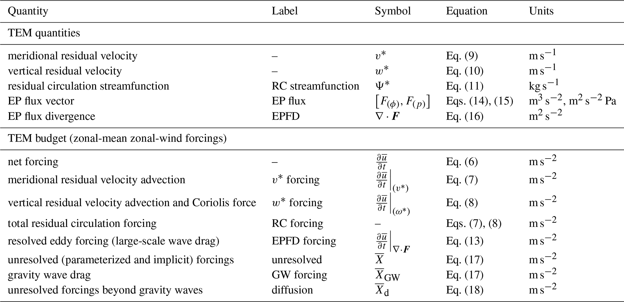
The philosophy behind the TEM equations of motion as a diagnostic tool for wave–mean flow interaction has been articulated in several foundational works (e.g., Edmon et al., 1980; Dunkerton et al., 1981; Andrews et al., 1983). For our purposes, the framework will allow us to identify the mechanisms that are responsible for volcanic-aerosol-induced changes to the zonal flow. Specifically, by applying the methods of Sect. 3.1 to $\stackrel{\mathrm{‾}}{u}$, we will identify statistically significant impacts on the zonal-mean zonal wind. We then separate the forcing of $\stackrel{\mathrm{‾}}{u}$ into the contributions from the residual circulation (Eqs. 7 and 8), from resolved eddy forcing (Eq. 13), and parameterized forcings and dissipation (Eq. 18). By statistically comparing the closed TEM budgets of each ensemble, we may diagnose which of these dynamical mechanisms control the separation between the volcanic and counterfactual simulations at certain locations and times. The important quantities and equations used in this procedure are summarized in Table 1, which may be useful in reading the later figures.

Table 1 Essential quantities of the TEM framework and TEM zonal momentum budget. The second column (“Label”) refers to the labels given to the corresponding quantity in figure titles and legends throughout this work. Quantities without a label are labeled with either their name (first column) or their symbol. Units provide the SI units, though different units may appear in figures. All quantities are computed on daily-averaged simulation data, except for the GW forcing and diffusion components of the TEM budget, which are computed on monthly-averaged data.

Note that all zonal averages throughout this paper are taken by the spectral spherical-harmonic method described in Appendix B, which avoids the need to remap the data from the E3SMv2 native cubed-sphere grid to a structured latitude–longitude format. In computing Eq. (18), the total tendency $\partial \stackrel{\mathrm{‾}}{u}/\partial t$ was not available to us as a model output in the simulation ensembles, and so it is constructed from the daily-mean $\stackrel{\mathrm{‾}}{u}$ by a first-order finite forward difference. Meridional and vertical derivatives are computed with a second-order centered finite difference. See Appendix A for details.

4 Reference state

4.1 Midlatitudes

In order to establish the behavior of the unforced simulations during the Pinatubo period, Fig. 1a–d show the seasonal zonal-mean zonal-wind structure for a single year of the CF ensemble mean, spanning June 1991 to June 1992. The stratospheric winds in the E3SMv2-SPA model appear to be broadly consistent with climatological averages deduced from the ERA5 reanalyses dataset (Fig. 2 in Butchart, 2022), with the SH wintertime polar vortex reaching maximum wind speeds in excess of 80 m s⁻¹ toward the model top and near 60° S and the NH polar vortex reaching speeds above 50 m s⁻¹ near 60° N. In each summer hemisphere, easterlies peak at 30–40 m s⁻¹ near 20° N and 20° S. These wind speeds are slightly low for the SH and slightly high for the NH with respect to the reanalysis climatology but are well within the range of observed variability (Fig. 8 in Butchart, 2022). There is similar accuracy in the tropospheric jets.

In addition, EP flux vectors and contours of the residual circulation streamfunction are plotted over the seasonal winds in Fig. 1a–d. Negative values in streamfunction (dashed contours) indicate counter-clockwise circulation on the meridional plane and vice versa for positive values (solid contours). The zero line between these regions is drawn in bold. Qualitatively, this shows Equator-to-pole overturning cells in the lower stratosphere and below and a single pole-to-pole circulation from summer-to-winter hemisphere during the solstitial seasons. These two regimes represent the advective components of the well-known shallow and deep branches of the BDC, respectively (Birner and Bönisch, 2011; Butchart, 2014).

The EP flux vectors show the relative magnitude and direction of resolved wave propagation in the meridional plane (Edmon et al., 1980; Andrews, 1987). In the summer hemisphere, wave activity forced by surface processes is largely constrained below the tropopause (e.g., Fig. 1a, NH), since the stratospheric easterlies aloft prevent the vertical propagation of Rossby waves (Charney and Drazin, 1961). During the following autumn, the development of upper-level westerlies acts as a valve for wave propagation into the stratosphere (e.g., Fig. 1b, NH). This persists through the winter, when stratospheric wave activity (and thus, zonal-wind variability) is at its highest (e.g., Fig. 1c, NH).

The seasonal TEM momentum balance is shown in Fig. 1e–h at 3 hPa (winter vortex core) and 30 hPa (lower vortex edge). Forcing by the EPFD, the residual circulation, parameterized gravity wave drag, subgrid diffusion, and their sum are plotted as functions of latitude, along with the CF ensemble mean $\stackrel{\mathrm{‾}}{u}$. Scaling of the vertical axis is unique in each panel. This reveals the familiar result (e.g., Andrews et al., 1983) that the net tendency $\partial \stackrel{\mathrm{‾}}{u}/\partial t$ in the stratosphere is due to a relatively small imbalance between negative wave-driven forcing (dissipation and breaking of resolved large-scale waves and parameterized gravity waves) and positive forcing by the residual circulation (Coriolis torque and advection of momentum).

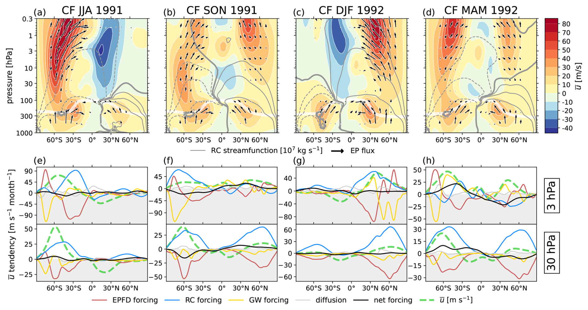
Figure 1 Seasonal zonal-wind and TEM momentum balance for the first year of the CF ensemble mean. (a–d) $\stackrel{\mathrm{‾}}{u}$ averaged over 3-month seasons in contours of 10 m s⁻¹, with EP flux vectors, gray Ψ^* contours, and the tropopause overplotted as a thick, faint white contour. The EP flux vectors are scaled following Jucker (2021). The Ψ^* contours are drawn at 30, 100, and 500 in units of 10⁷ kg s⁻¹ on each side of zero (bold contour). Negative contours are dashed. (e–h) Seasonal contributions to $\partial \stackrel{\mathrm{‾}}{u}/\partial t$ in [m s⁻¹ per month] from the EPFD (red solid), the residual circulation (blue solid), gravity waves (gold solid), and diffusion (thin gray solid) as functions of latitude at 3 hPa (top panels) and 30 hPa (e–h). Also shown is the net tendency (black solid), as well as $\stackrel{\mathrm{‾}}{u}$ itself (thick green dashed) in [m s⁻¹]. The negative tendency (and wind speed) domain is shaded in light gray. Note that each panel of (e)–(h) has unique scaling of the vertical axis, such that all curves are contained within the plotting region.

In the summer hemisphere, both the wave-driven and residual circulation forcing magnitudes are low, and the compensation between them is nearly complete (e.g., Fig. 1e, NH). The result is mild easterly wind speeds with low variability. In the winter hemisphere (e.g., Fig. 1g, NH), approximate balance between the forcing terms remains, but the relative contributions are much larger. The result is a strong polar jet. The equinoctial seasons serve as the transitions between the two quasi-steady states found in the summer and winter stratosphere, at which time the force balance must break, and the total mean forcing on $\stackrel{\mathrm{‾}}{u}$ departs from zero (Fig. 1f, h). In the autumnal hemisphere, net positive forcing arises as the polar vortex is spun up by the Coriolis torque of the strengthening meridional residual velocity, while in the vernal hemisphere, net negative forcing results as wave drag erodes the vortex.

Note that in both winter hemispheres at 3 hPa (Fig. 1e, SH and Fig. 1g, NH) there tends to be a sign change in the EPFD on each side of the polar vortex, such that wave breaking and dissipation (EPFD <0) occur equatorward, in the surf zone (McIntyre and Palmer, 1984), and wave divergence (EPFD >0) occurs poleward. This is qualitatively consistent with some reanalysis climatology results, e.g., ERA-Interim (Díaz-Durán et al., 2017). The parameterized gravity wave drag (yellow curve) in the model tends to exhibit the opposite behavior.

At 30 hPa, well below the vortex peak, there is broad negative EPFD from the midlatitudes to the poles. This westward wave driving is about a factor of 2 larger in magnitude in the NH than the SH due to the continental land masses – an effect which might have the capacity to trigger a breakdown of the vortex (Baldwin et al., 2021) in a different realization.

4.2 Tropics

The tropical zonal-mean zonal wind averaged over 5° S–5° N in the CF ensemble mean is shown in Fig. 2 for the full 8-year simulated time period. In Fig. 2a, the initial QBO phase is easterly, and its first cycle has a period of approximately 24 months with peak winds of about −10 and 7 m s⁻¹ in January of 1991 and 1992 respectively, at 30 hPa in the ensemble mean. This is weak by a factor of 2 to 3 compared to ERA5, which is a known bias of E3SMv2 (Yu et al., 2025).

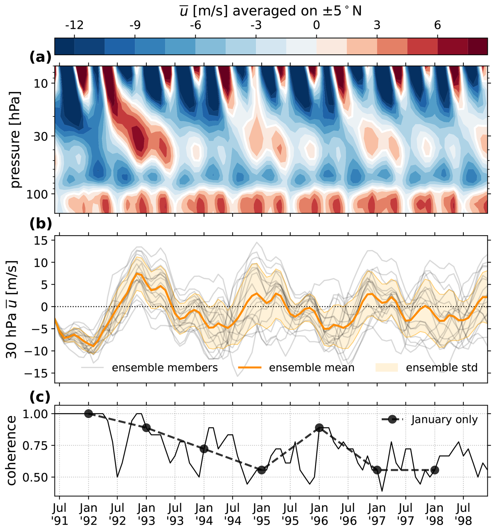
Figure 2 The QBO shown as $\stackrel{\mathrm{‾}}{u}$ averaged over [5°S, 5°N] for the CF ensemble mean. (a) Time–pressure plane centered on the lower stratosphere. (b) Zonal-wind time series at 30 hPa. The ensemble mean and standard deviation in $\stackrel{\mathrm{‾}}{u}$ is shown as a bold orange line and light orange shading, respectively. Individual ensemble members are shown as faint gray lines, and the zero line is dotted. (c) The ensemble coherence, defined as the fraction of ensemble members in agreement with the sign of the ensemble mean in panel (b). A bold dashed line with points displays the coherence evaluated only at each January.

In addition to a weak amplitude compared to reanalyses, the semi-annual oscillation (SAO) penetrates deeper into the stratosphere, and the descent of QBO phases is typically hastened in E3SMv2, resulting in a shortened period at fixed pressure. Yu et al. (2025) showed that the spectral density of the QBO computed over 1985–2015 at 20 hPa in E3SMv2 is approximately uniform in power from 20 to 30 months in period, with no distinct peak. For our realizations in E3SMv2-SPA, the QBO manifests with a period of about 24 months. This causes a seasonal phase lock, where maxima and minima in QBO wind speeds occur during alternating boreal winters.

Following the first cycle, the QBO signal in the ensemble mean weakens further, by an additional factor of ∼2. This weakening is explained by the increasing intra-ensemble spread, as the members diverge from their common initial condition, demonstrated at 30 hPa in Fig. 2b. Alternatively, Fig. 2c shows the 30 hPa ensemble “coherence”, or the fraction of the members which agree in sign with the ensemble mean. The coherence is variable, unsurprisingly dropping to 50 % whenever $\stackrel{\mathrm{‾}}{u}$ crosses zero. More useful is the January coherence (bold dashed line and points) which, because of the seasonal phase lock of the QBO in the model, shows the ensemble phase agreement during each easterly and westerly maximum. We observe that the January coherence drops below 80 % near July of 1993, and so for the remainder of this study we will focus only on this early 2-year period. In the midlatitudes, we should expect the ensemble coherence to fall off faster, though we will still conduct the analysis over this same period.

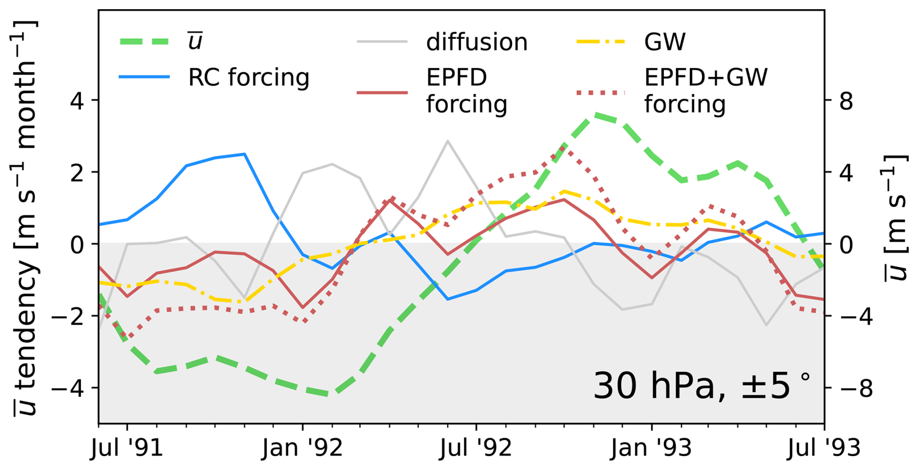
Figure 3 The TEM momentum balance of the QBO for the first 2 years of the CF ensemble mean, averaged over [5° S, 5° N] at 30 hPa. Shown are the contributions to $\partial \stackrel{\mathrm{‾}}{u}/\partial t$ in [m s⁻¹ per month] from the EPFD (red solid), gravity waves (gold dotted), the combined EPFD and gravity waves (red dotted), the residual circulation (blue solid), and diffusion (thin gray solid). Also shown is $\stackrel{\mathrm{‾}}{u}$ itself (thick green dashed) in [m s⁻¹], with values on the right vertical axis. The negative tendency or wind speed domain is shaded in light gray.

The TEM balance describing the QBO evolution at 30 hPa over the initial 2-year period is shown in Fig. 3. Curves show the monthly-mean time series of the forcing on $\stackrel{\mathrm{‾}}{u}$ by the EPFD and gravity waves, the residual circulation, and diffusion (these are the same data as in Fig. 1e–h before seasonal averaging but with the net forcing omitted). The sum of the EPFD and gravity wave drag is also drawn (red dotted line), which shows the usual result that wave driving is the dominant process controlling the QBO phase descent (Baldwin et al., 2001). However, momentum transport by vertically propagating tropical waves is actually much larger than the net motion of the QBO would suggest (peaking at ∼3 m s⁻¹ per month in NH autumn of 1992, while the net tendency is nearer to ∼1.3 m s⁻¹ per month), since it is partially canceled by the residual circulation (blue solid line), which hinders the descending phase (Dunkerton, 1997). As the Coriolis force is negligible at these latitudes, and v^* is small, this forcing can be interpreted primarily as a diabatic effect, where upwelling of momentum by w^* is in control (see streamfunction contours in Fig. 1). The result is positive (negative) forcing by the residual circulation in westerly (easterly) shear zones (as in, e.g., Brown et al., 2023).

5 Volcanic impact results

With an understanding of the seasonal TEM balance in the CF ensemble established, we now investigate disruptions to this balance by the Pinatubo aerosol forcing. Figure 4 shows the monthly-averaged global $\mathrm{\Delta }\stackrel{\mathrm{‾}}{u}$ for select months in the autumn of 1991, winter of 1992, and autumn of 1992 (panels a–c), as well as meridionally resolved impacts over 70° S–70° N as a function of time at 10 and 30 hPa (panels d, e). On all panels, the counterfactual winds are drawn in black contours every 10 m s⁻¹. Regions where the statistical significance of the impact is above 95 % are enclosed by a bold white contour, and regions below 95 % are marked with white hatching.

Midlatitude and tropical impacts are discussed in Sect. 5.1 and 5.2, respectively. The strategy is to (1) identify localized regions of significant $\mathrm{\Delta }\stackrel{\mathrm{‾}}{u}$ in space and time; (2) over the each identified region, decompose $\mathrm{\Delta }(\partial \stackrel{\mathrm{‾}}{u}/\partial t)$ into the TEM form of Eq. (6); and (3) analyze the imbalance between the impact of the TEM terms. If the result of this process is a set of TEM impacts which are themselves statistically significant, then we will consider the specific mechanism in control of the associated $\mathrm{\Delta }\stackrel{\mathrm{‾}}{u}$ to have been found.

In the midlatitudes, this process amounts to answering the following question: if thermal wind balance is to be approximately maintained after a source of external forcing is introduced, then what processes govern the required adjustments to the zonal wind to that end? From a TEM perspective, it might be assumed that the residual circulation and large-scale wave drag conspire in this purpose, but as we will show, the quantitative details of this balance change notably with at least season and latitude.

This type of analysis has precedent in the literature, most notably Bittner et al. (2016) and Toohey et al. (2014), but we are not aware of another work on volcanic aerosol forcing that attempts to give a complete accounting of the closed TEM budget in this way. We take some inspiration from similar closed-budget analyses that have been done for climate trends in tracer distributions, e.g., Abalos et al. (2013, 2017, 2020).

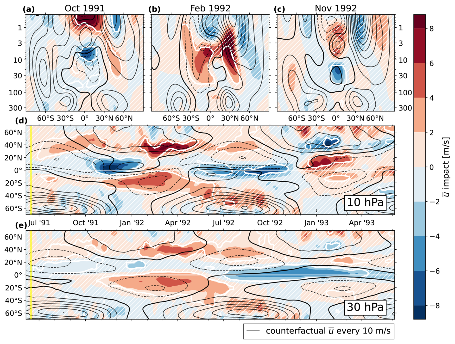
Figure 4 The ensemble-mean $\mathrm{\Delta }\stackrel{\mathrm{‾}}{u}$ as filled contours (color scale), with the CF ensemble-mean $\stackrel{\mathrm{‾}}{u}$ overplotted as black contours, drawn every 10 m s⁻¹, with negative contours dashed and the zero line in bold. A bold white contour is drawn at 95 % significance, with the $\mathrm{\Delta }\stackrel{\mathrm{‾}}{u}$ p value computed as in Sect. 3.1. Regions of insignificance are filled with white hatching. The upper three panels show the latitude–pressure plane for time averages over (a) October 1991, (b) February 1992, and (c) November 1992. The lower two panels show the time–latitude plane for pressure levels at (d) 10 hPa and (e) 30 hPa. In panels (d) and (e), a vertical yellow line shows the time of eruption, and a faint white line is drawn on the Equator.

5.1 Impacts in the surf zone and polar vortex

Figure 4d and e show that until 2 years post-eruption, essentially all stratospheric $\stackrel{\mathrm{‾}}{u}$ impacts outside of the tropics are westerly in nature, consistent with aerosol-driven enhancements of the meridional temperature gradient. These features correspond to either zonal acceleration or deceleration with respect to the reference, depending on the season.

The significant response begins near 10 hPa in both hemispheres (Fig. 4d). In the Northern Hemisphere, a westerly impact of ∼ 3 m s⁻¹ develops near 30° N, decelerating easterly winds (black dashed contours) from July through the end of the NH summer of the eruption. This impact moves poleward toward 60° N throughout autumn, acting to hasten the spin-up of the polar vortex along its equatorward edge, before becoming insignificant in early November. The vertical structure averaged over October 1991 is given in Fig. 4a, which suggests that this feature is perhaps part of a subtle equatorward shift of the vortex, given the accompanying easterly impact near the vortex core above 1 hPa. We will refer to this impact signature as the “summer response” (SR). Note that a similar summer response occurs again from July to October of 1992 near 30° N, as well as in the Southern Hemisphere between December and April 1992, albeit at lower latitudes.

Following the 1991 SR is a stronger westerly impact of up to ∼ 6 m s⁻¹ occurring at both 10 and 30 hPa near 40° N, between January and May 1992 (Fig. 4d, e). This impact serves to accelerate westerlies in the surf zone (equatorward edge of the polar vortex). Figure 4b shows the vertical structure averaged over February of 1992, in which we again see easterly impacts near and poleward of the vortex core, indicative of equatorward vortex shift (though it is insignificant). We will refer to this impact as the “winter response” (WR), and we identify this response most closely with the claims of an “accelerated vortex region” that are well represented in the literature, as discussed in Sect. 1. A similar (but insignificant) response also occurs in the Southern Hemisphere near 50° S between June and October 1992.

The summer and winter responses are summarized in Fig. 5, which shows the separation of the LV and CF ensembles in one dimension as $\stackrel{\mathrm{‾}}{u}$ and $\mathrm{\Delta }\stackrel{\mathrm{‾}}{u}$ at 20 hPa, averaged over 30–50° N. Also plotted are the 95 % confidence intervals on the ensemble means and the impact, as well as curves at 2 standard deviations. In the lower panel, the confidence interval is shaded in green where the impact is significant, which clearly shows the 1991 SR, 1992 WR, and 1992 SR. This view illustrates that the relatively strong wintertime stratospheric variability in the vortex region sets a kind of lower bound on the forcing magnitude that is required to illicit a significant response, which our simulations are only just managing to overcome. In the summertime quiescent stratosphere, on the other hand, the noise floor is much lower, and so even small impacts can be detected. This is consistent with the findings of previous work that demonstrated a statistically weak response from Pinatubo-like forcing, even for much larger ensemble sizes (Bittner et al., 2016).

For the remainder of this section, our analysis will be restricted to the Northern Hemisphere, since those impacts occur earlier and with more significance and have more representation in the literature. There is some suggestion of an easterly impact in boreal winter of 1993 (Fig. 4d), but it is largely insignificant. Hence, we will also restrict the analysis of this section to the first 12–16 months post-eruption.

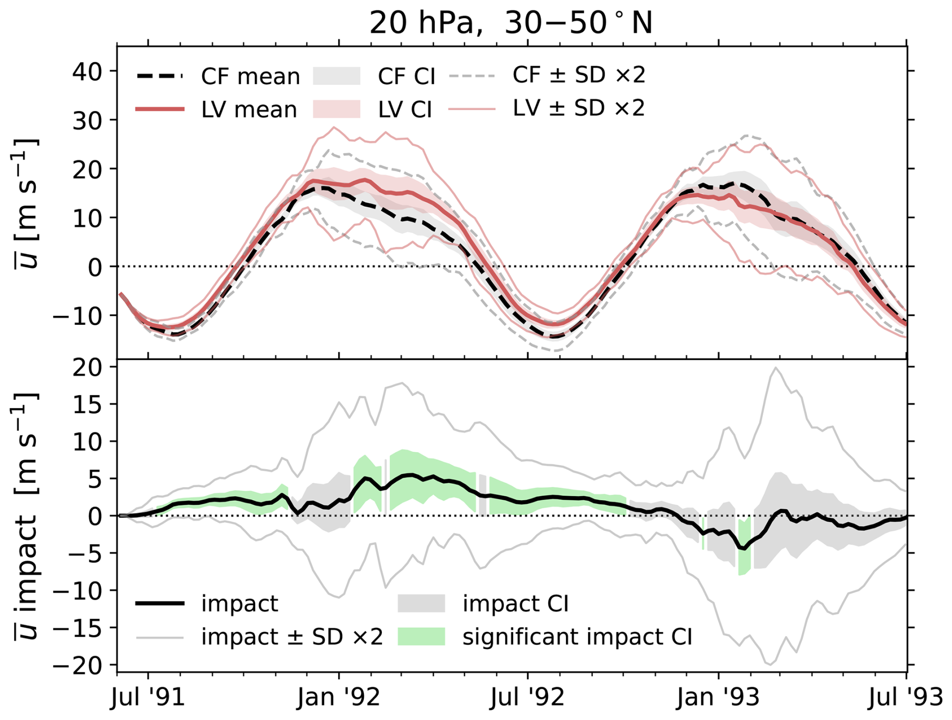
Figure 5 Time series of the CF ensemble-mean $\stackrel{\mathrm{‾}}{u}$ and LV ensemble-mean $\stackrel{\mathrm{‾}}{u}$ (upper panel) as well as the ensemble-mean $\mathrm{\Delta }\stackrel{\mathrm{‾}}{u}$ (lower panel) at 20 hPa, averaged over 30–50° N. In both panels, shaded bands give the confidence intervals, as computed in the way of Sect. 3.1, and thin lines give 2 standard deviations on each side of the mean. In the lower panel, the confidence interval is shaded in light green where the impact is statistically significant at the 95 % level.

5.1.1 TEM balance of the surf zone and polar vortex

We now investigate the impacts to the TEM balance associated with both the summer and winter midlatitude responses. Figure 6 picks out the 30–50° latitude band at 10 hPa from Fig. 4d and reproduces it in its panel (a). Panel (b) shows the vertically resolved meridional average over this band. Over this domain, in addition to $\mathrm{\Delta }\stackrel{\mathrm{‾}}{u}$, we also obtain the impact (as Eq. 1) of the net tendency $\partial \stackrel{\mathrm{‾}}{u}/\partial t$, the large-scale wave drag (Eq. 13), the residual circulation forcing (Eqs. 7 and 8), gravity wave drag, and diffusion (Eq. 18). We then define time windows which span the 1991 SR, 1992 WR, and 1992 SR. Next, we individually integrate the TEM forcing terms from the left (time t₀) to the right (time t₁) ends of each window, all of which are given a common initial condition of $\stackrel{\mathrm{‾}}{u}\left(t_{\mathrm{0}}\right)$ as evaluated in the LV ensemble mean.

In this way, the sum of the integrated TEM impacts is identical to the integration of the $\mathrm{\Delta }(\partial \stackrel{\mathrm{‾}}{u}/\partial t)$, which in turn is identical to the observed $\mathrm{\Delta }\stackrel{\mathrm{‾}}{u}$. This procedure is described in detail in Appendix A, and the result is shown in Fig. 6c–e. The intention is to visualize the accumulated contribution to the observed $\mathrm{\Delta }\stackrel{\mathrm{‾}}{u}$ by each of the large-scale TEM processes. In other words, each curve shown in panels (c)–(e) shows the anomalous evolution of the wind in absence of all other forcings, given the shared initial condition. This is preferable to showing the forcing impacts themselves, since those often change sign on small temporal scales, and thus the noise would visually dominate over the meaningful trend.

Each integration time window is shown as a highlighted yellow-green strip in panel (b) at 10 hPa. The integrated tendency contributions are shown in panel (c) for the 1991 SR, panel (d) for the 1992 WR, and panel (e) for the 1992 SR. It is immediately apparent that while these westerly impacts appear similar from a thermal-wind perspective, they are in fact brought about by different mechanisms.

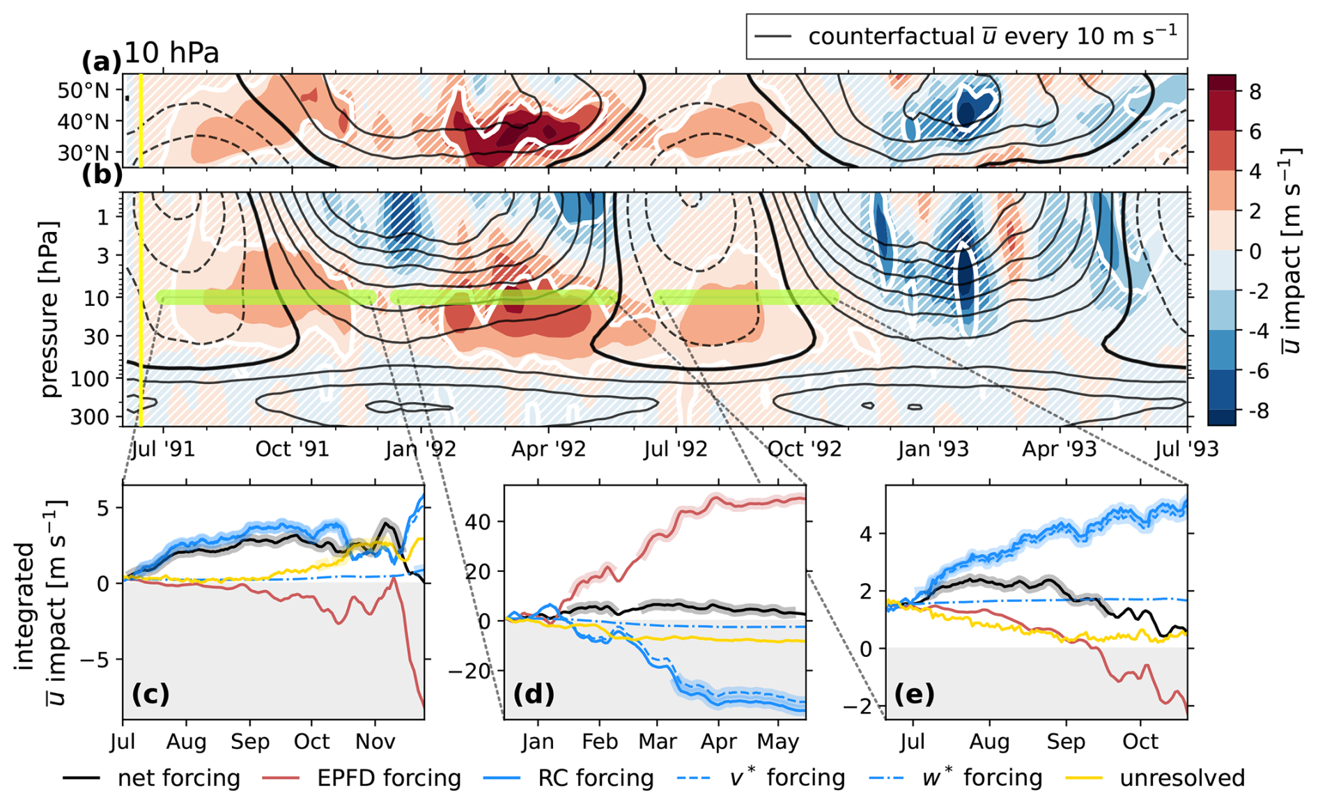
Figure 6 Vertical structure of the midlatitude zonal-wind impacts and the TEM balance impact at 10 hPa. Panels (a) and (b) show the ensemble-mean $\mathrm{\Delta }\stackrel{\mathrm{‾}}{u}$ as filled contours (color scale), with the CF ensemble mean $\stackrel{\mathrm{‾}}{u}$ overplotted as black contours, drawn every 10 m s⁻¹, with negative contours dashed and the zero line in bold. A bold white contour is drawn at 95 % significance, with the $\mathrm{\Delta }\stackrel{\mathrm{‾}}{u}$ p value computed as in Sect. 3.1. Regions of insignificance are filled with white hatching. Panel (a) shows the latitude band from 25 to 55° N at 10 hPa, reproduced from Fig. 4b. Panel (b) shows the meridional mean over 30–50° N, from 400 to 0.5 hPa, for 2 years following the eruption (which is indicated with a vertical yellow line). In panels (c)–(e), curves show the integrated forcing impact by the EPFD (red solid), by w^* advection (dash-dotted blue), by v^* advection and the associated Coriolis force (dashed blue), and by $\stackrel{\mathrm{‾}}{X}={\stackrel{\mathrm{‾}}{X}}_{\text{GW}}+{\stackrel{\mathrm{‾}}{X}}_d$ (yellow solid). Also shown is the cumulative residual velocity forcing (blue solid) and the total forcing (black solid). The curves are backed by a thick shading of a matching color where they are statistically significant. Each term has units of m s⁻¹ after time integration. The total forcing curve (black solid) matches the data on the color scale in the corresponding highlighted region of panel (b). These data are computed according to Appendix A. The negative domain is shaded.

The summertime responses of 1991 and 1992 (panels c and e) are characterized by a deficit of large-scale wave forcing and a surplus of forcing by the residual circulation. While the magnitude of impact on each of these effects is comparable, it is the residual-circulation forcing that is favored in the imbalance and is ultimately responsible for the manifest $\mathrm{\Delta }\stackrel{\mathrm{‾}}{u}$. Specifically, the forcing is almost entirely due to the impact on the meridional component, Δv^*, and can be interpreted primarily as a Coriolis-driven acceleration, while Δw^* is very small (as expected in the extratropics). Toward the end of the integration time windows, it appears that an increasingly negative Δ(EPFD) eventually dominates and brings the summer responses to an end. Impacts on gravity wave and diffusion forcing play a more minor role and have opposite signs in 1991 and 1992.

On the other hand, the wintertime response is primarily wave-driven (panel d). From January to April 1992, Δ(EPFD) and Δv^* are both large (nearly an order of magnitude larger than the previous summer), though the imbalance favors the former. This drives a net westerly acceleration. By spring of 1992, the TEM forcings are re-aligning with the reference runs (the integrated tendency curves are flattening), and the restored balance brings the winter response to an end.

In order to clarify the nature of these mechanisms of impact, Figs. 7, 8, and 9 show the complete TEM budget for the zonal-wind impact $\mathrm{\Delta }\stackrel{\mathrm{‾}}{u}$ in the meridional plane for select monthly means during the 1992 WR, 1991 SR, and the 1992 SR, respectively. In each of these figures, panel (a) shows $\mathrm{\Delta }\stackrel{\mathrm{‾}}{u}$, $\mathrm{\Delta }\stackrel{\mathrm{‾}}{u}$ significance, and ${\stackrel{\mathrm{‾}}{u}}^{\text{CF}}$, in the way of Fig. 4. Panels (b)–(e) then show the impacts of the TEM forcing terms, and their significance, while panels (f)–(i) show the reference forcings from the CF ensemble. In panels (f) and (b), the CF EP flux vectors and their impacts are shown, respectively. Likewise, in panels (g) and (c), the CF Ψ^* tangent vectors and their impacts are shown, which have been scaled using a method detailed in Appendix C. In all panels (b)–(i), the significance contours from panel (a) are reproduced in black, for spatial reference. The monthly averaging periods were informed by Fig. 6, chosen such that we analyze times when the forcing impacts are strong (i.e., integrated curves in Fig. 6c–e are steep).

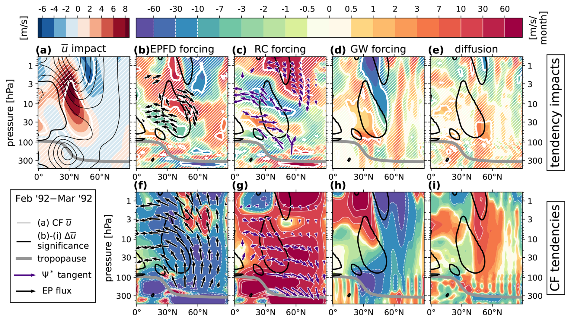
Figure 7 The complete TEM budget in the Northern Hemisphere meridional plane from 500 to 0.5 hPa, averaged from 1 February 1992 to 1 March 1992. (a) The ensemble-mean $\mathrm{\Delta }\stackrel{\mathrm{‾}}{u}$ as filled contours (red/blue color scale), with the CF ensemble-mean $\stackrel{\mathrm{‾}}{u}$ overplotted as black contours, drawn every 10 m s⁻¹, with negative contours dashed and the zero line in bold. For every other vertical pair of panels, the top and bottom panels show the ensemble-mean impact and CF ensemble-mean of a variable as filled contours (rainbow color scale). Specifically, panels (b) and (f) show the EPFD forcing (Eq. 13). Black vectors drawn in these panels show the significant ensemble-mean impact and the CF ensemble-mean EP flux vectors (Eqs. 14, 15), respectively, scaled according to Jucker (2021). The vector lengths are additionally log-scaled equally in length, in order to effectively visualize the vector directions. Panels (c) and (g) show the residual-circulation forcing (Eqs. 7 and 8). Purple vectors drawn in these panels show the significant ensemble-mean impact and the CF ensemble-mean Ψ^* tangent vectors (Eq. 11), respectively, scaled according to Appendix C. For both Ψ^* and the EP flux, vectors near and below the tropopause are removed. Panels (d) and (h) show the gravity-wave forcing. Panels (e) and (i) show the forcing by diffusion (Eq. 18). On all panels, regions of 95 % statistical significance are enclosed with a bold white contour for the variable plotted on the color scale, and regions of insignificance are filled with white hatching. For spatial reference, the significance contour of the net impact $\mathrm{\Delta }\stackrel{\mathrm{‾}}{u}$ (bold white contour in panel a) is reproduced as a solid black contour in all other panels. Also plotted on all panels is the tropopause, as a bold gray curve. In the rainbow color scale used for the tendencies, thin solid (dashed) white contours are drawn between all values larger than positive (negative) 10 m s⁻¹ per month in magnitude.

Figure 7 reiterates that the wintertime acceleration of westerly winds at the equatorward vortex edge is primarily a consequence of perturbed wave activity. Panel (b) shows a statistically significant surplus of large-scale wave drag (negative forcing impact) at the lower, equatorward edge of the region of significance in $\mathrm{\Delta }\stackrel{\mathrm{‾}}{u}$ and a deficit of drag aloft (positive forcing impact). Comparing the vectors of panels (b) and (f) reveals the cause for this effect. Relative to the CF ensemble mean, vertical and equatorward wave propagation is decreased near 50° N and 10 hPa, while it is enhanced near 30° N and 30 hPa. This result is exactly the “wave deflection” mechanism proposed by Bittner et al. (2016), where enhanced westerlies near 30° N alter the background condition for wave propagation in the surf zone, serving to steer Rossby waves away from the vortex. With those waves breaking at relatively lower latitudes, the vortex experiences less drag and higher wind speeds. In our simulations, this effect does not extend to the vortex core, but the mechanism appears to be the same.

At the same time, the residual circulation contribution to the forcing impact opposes the CF condition at 10 hPa but reinforces it at 30 hPa and near the model top. Comparing the vectors of panels (c) and (g), this appears to simultaneously suggest (1) a localized deceleration of the midlatitude shallow branch and (2) an acceleration of the deep branch of the advective BDC. In addition, panels (d), (e), (h), and (i) show that while positive impacts to the forcing by gravity wave drag and diffusion are present, they are minor contributors to the net response.

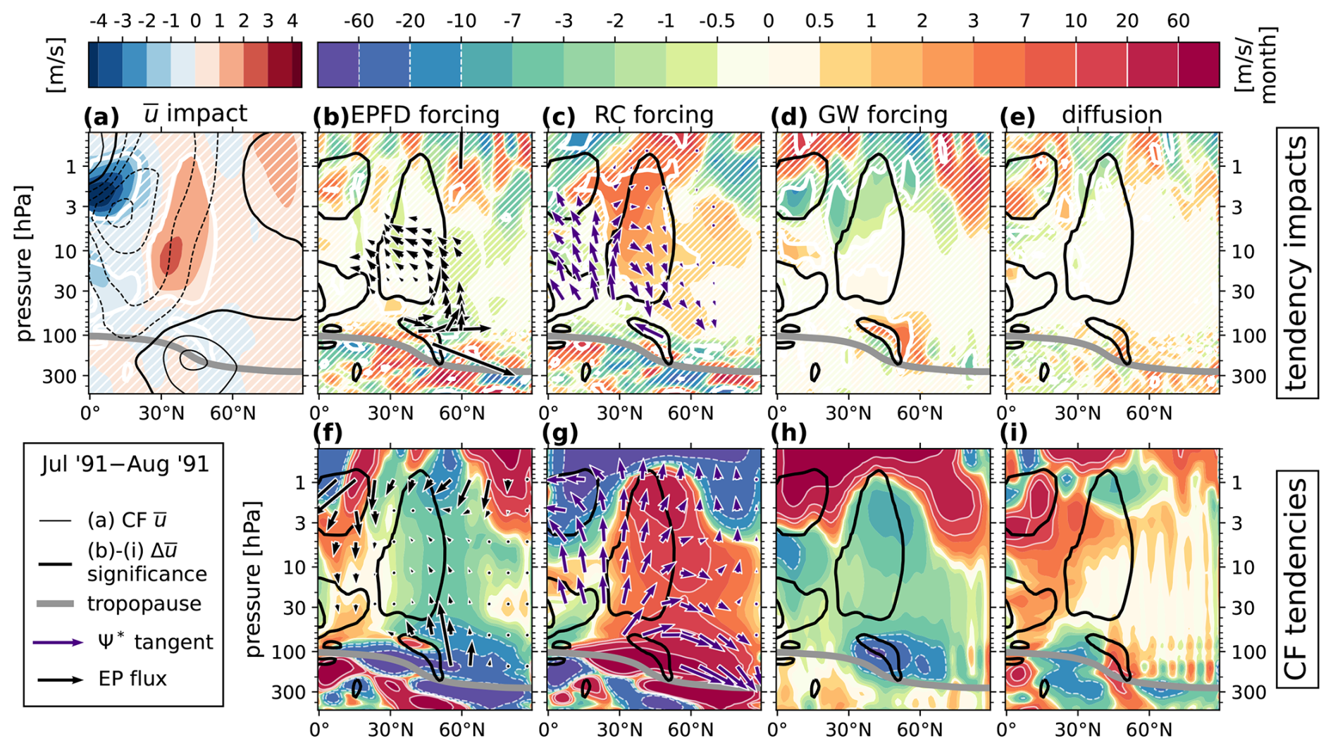
Figure 8 The complete TEM budget in the Northern Hemisphere meridional plane from 500 to 0.5 hPa, averaged from 1 July 1991 to 1 August 1991. See the caption of Fig. 7 for full panel descriptions, considering the following modifications: in panel (b), the EP flux vectors are scaled in length to an order of magnitude smaller than the CF vectors in panel (f), and both set of vectors are linearly scaled in length rather than log-scaled. In panel (c) the Ψ^* tangent vectors are scaled to 2 orders of magnitude smaller than the CF vectors in panel (g) in length, and both sets of vectors are log-scaled.

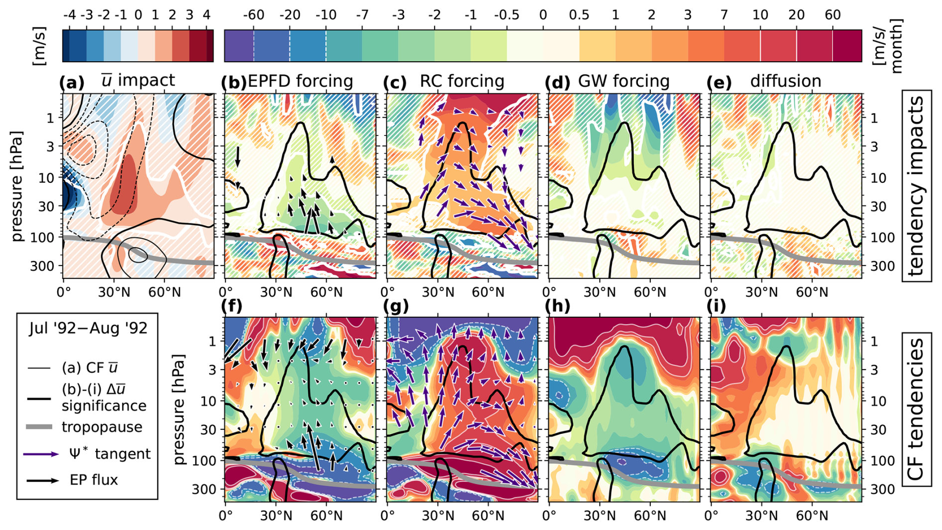
Figure 9 The complete TEM budget in the Northern Hemisphere meridional plane from 500 to 0.5 hPa, averaged from 1 July 1992 to 1 August 1992. See the caption of Fig. 7 for full panel descriptions, considering the following modifications: in panel (b), the EP flux vectors are scaled in length to an order of magnitude smaller than the CF vectors in panel (f), and both sets of vectors are linearly scaled in length rather than log-scaled. In panel (c) the Ψ^* tangent vectors are scaled to 2 orders of magnitude smaller than the CF vectors in panel (g) in length, and both sets of vectors are log-scaled.

Figures 8 and 9 show the analogous results for the 1991 SR and 1992 SR, which reiterate that the summertime westerly impacts are primarily a consequence of enhanced Coriolis torque from positive impacts on v^*. This is demonstrated in panel (c), which shows a strengthened poleward meridional circulation (vector fields) and an associated positive forcing impact over the entire region of $\mathrm{\Delta }\stackrel{\mathrm{‾}}{u}$ significance. These anomalous circulation cells project strongly onto the counterfactual residual circulation (panel g) at 10 hPa and below, which we interpret as an acceleration of the shallow branch of the advective BDC. During the summer of 1991, this acceleration is limited to the subtropics but has expanded to the pole by the summer of 1992.

Meanwhile, in panels (b), (f), (d), and (h), we see that impacts to both resolved and unresolved wave drag either are weak or oppose the sign of the net westerly impact. In the case of resolved Rossby waves, the EP flux vector impacts shown in panel (b) indicate that expanded regions of westerly $\stackrel{\mathrm{‾}}{u}$ near 30 hPa and below are allowing vertical wave propagation, which would otherwise have been prevented by the presence of easterlies (especially in Fig. 9).

5.2 Impacts in the tropics

Figure 4d and e show that the significant impacts to the zonal circulation in the tropics arise and persist over a much longer timescale than those in the midlatitudes. The first of these occur in the NH autumn 1991 at 10 hPa (Fig. 4d) as strong easterly, followed by westerly impacts between 20° S–20° N. The October 1991 mean given in Fig. 4a shows that this feature is paired with a complementary tropical impact above 1 hPa, which may be understood as a lag in the descent of the westerly phase of the SAO. For the remainder of this study, we choose to ignore the SAO impacts for brevity and instead focus on the response of the QBO.

In our simulations, the Pinatubo eruption occurs during a descending easterly QBO phase, with easterly wind shear (see Fig. 2). This state persists for around 6 months, at which point a westerly shear develops in January 1992, and westerly winds descend to 30 hPa by July 1992. Figure 4e shows that a significant positive $\mathrm{\Delta }\stackrel{\mathrm{‾}}{u}$ occurs in the tropics from December 1992 to May 1992, and subsequently a significant negative $\mathrm{\Delta }\stackrel{\mathrm{‾}}{u}$ occurs from July 1992 to April 1993. We will refer to these features as the “westerly response” and the “easterly response”, respectively. Both the westerly and easterly responses oppose their simultaneous QBO phase. Figure 4b suggests that the westerly response is a part of a broader summer impact in the low latitudes of the SH, while panel (c) shows that the easterly response is a localized feature which alters the QBO in particular. Together, we interpret these impacts as a significant (yet subtle) weakening of the QBO during the 2-year post-eruption period.

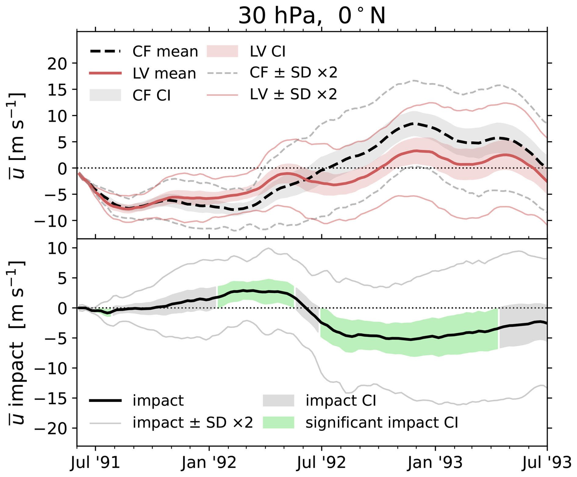
Figure 10 Time series of the CF ensemble-mean $\stackrel{\mathrm{‾}}{u}$ and LV ensemble-mean $\stackrel{\mathrm{‾}}{u}$ (upper panel) as well as the ensemble-mean $\mathrm{\Delta }\stackrel{\mathrm{‾}}{u}$ (lower panel) at 30 hPa, averaged over 5° S–5° N. In both panels, shaded bands give the confidence intervals, as computed in the way of Sect. 3.1, and thin lines give 2 standard deviations on each side of the mean. In the lower panel, the confidence interval is shaded in light green where the impact is statistically significant.

This QBO weakening is seen clearly in Fig. 10, which shows the separation of the LV and CF ensembles in one dimension as $\stackrel{\mathrm{‾}}{u}$ and $\mathrm{\Delta }\stackrel{\mathrm{‾}}{u}$ at 30 hPa, averaged over 5° S–5° N. The standard deviation and confidence intervals are analogous to those shown in Fig. 5. This indicates that the easterly and westerly QBO phases are weakened by ∼ 3 and ∼ 5 m s⁻¹, respectively (which approaches 50 % of the CF ensemble mean values). The arrival of the westerly phase at 30 hPa also appears delayed by ∼2–3 months.

5.2.1 TEM balance of the tropics

We now investigate the impacts to the TEM balance associated with the weakened QBO. Figure 11 picks out the 5° S–5° N latitude band from Fig. 4e and reproduces it in its panel (a). Panel (b) shows the vertically resolved zonal-wind impacts averaged over this band. In the same way as Fig. 6, the integrated impacts of the individual TEM forcing terms are shown as functions of time over two targeted time windows. The first window (panel c) is positioned to study the TEM imbalance, which generates the westerly $\mathrm{\Delta }\stackrel{\mathrm{‾}}{u}$ during the easterly QBO phase. The second window (panel d) is positioned to show the TEM imbalance which drives the transition from a westerly to easterly $\mathrm{\Delta }\stackrel{\mathrm{‾}}{u}$, as the westerly QBO phase descends.

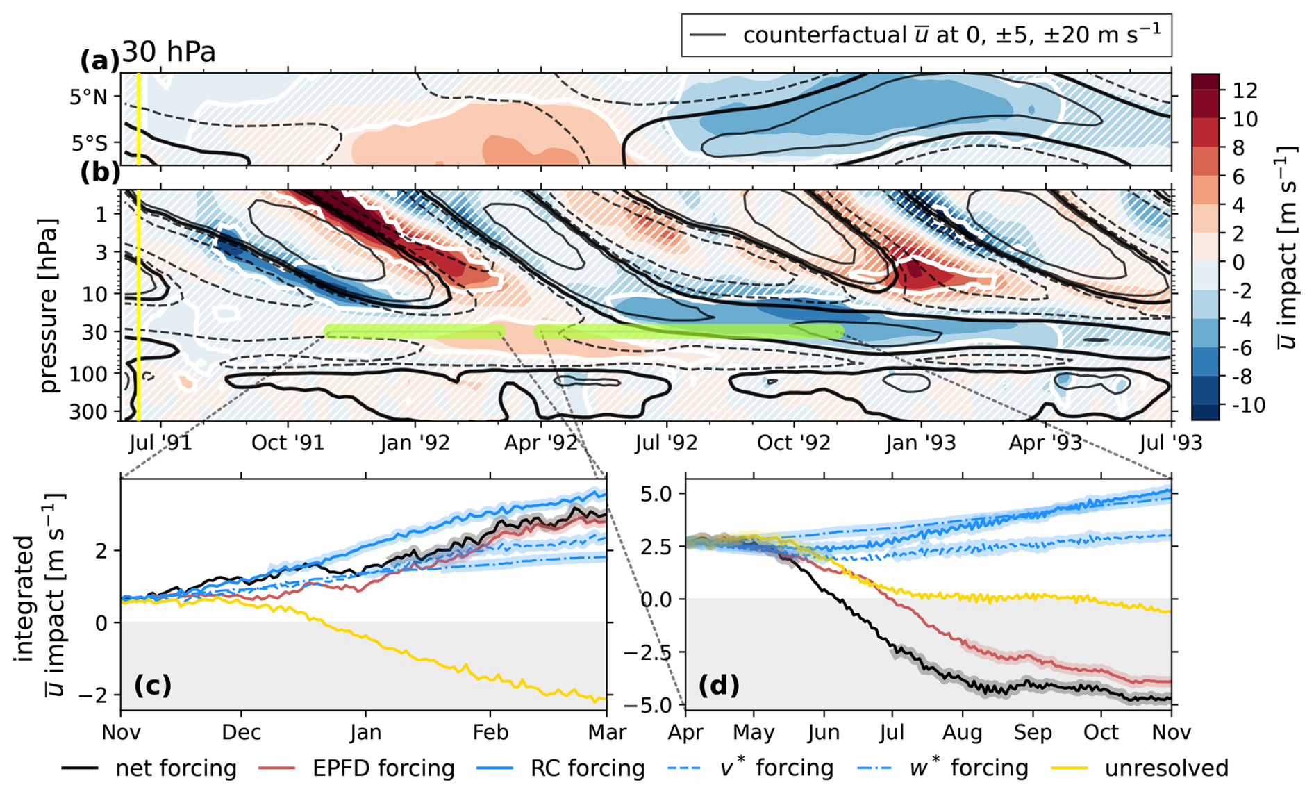
Figure 11 The same as Fig. 6 with the following modifications: panels (a), (c), and (d) are shown for the 30 hPa level. In panels (b), (c), and (d), the latitude band average is taken over 5° S–5° N. The CF $\stackrel{\mathrm{‾}}{u}$ contours in panels (a) and (b) are drawn at 0, ±5, and ± 20 m s⁻¹.

Figure 11c indicates that the westerly response is driven by some combination of decreased large-scale wave drag (a positive EPFD impact) and an increased forcing by the residual circulation, though this effect is opposed by unresolved sources, implying enhanced gravity wave drag. Because of the high-Rossby-number environment in the tropics, forcing by the residual circulation is primarily advective. There are approximately equal contributions from v^* and w^*, as the zero line of the streamfunction Ψ^* is generally located far from the Equator at 30 hPa except near the equinoxes (see Fig. 1a–d). On the other hand, Fig. 11d shows that the transition from the westerly response to the easterly response, and thus the opposition to the descent of the westerly QBO phase, is due primarily to enhanced resolved and unresolved wave drag at 30 hPa and only has an mild inhibiting contribution from residual circulation advection.

For a more complete picture of these mechanisms of impact, we performed an analysis of the complete TEM budget and its associated impacts in the meridional plane, averaged over 1-month periods, exactly analogous to that presented in Sect. 5.1.1. The averaging periods were again chosen to align with times of most rapid change in Fig. 11c and d (i.e., strongest TEM tendency impacts). These are shown in Figs. S1 and S2 in the Supplement of this article. The main finding was further evidence that an increase in large-scale and gravity wave drag drives the transition from the westerly to easterly response, in agreement with Fig. 11. We did not pursue this further and leave the task of examining the volcanic modification of large-scale tropical wave activity to future work, a subject which has received much less attention in the literature than the comparable midlatitude problem.

6 Discussion of comparable results in the literature

As noted in Sect. 5.1.1, the wintertime wave-deflection mechanism that we have identified is consistent with that proposed by Bittner et al. (2016). In that study, the effect is showcased for a much larger 55 Tg eruption. The authors noted, but did not show, that the effect was also detectable in their Pinatubo-sized eruption simulations but was less robust. The fact that we are able to robustly identify the wave deflection for a 10 Tg eruption may be due to various factors. For example, the model employed by Bittner et al. (2016) was described as showing excessive interannual variability compared to observations, which, as they suggest, “masks the response to the forcing of the volcanic aerosols”. To demonstrate this, they show that while a 55 Tg eruption was able to force both a positive anomaly in the mean and a negative anomaly in the variability of the vortex region, a Pinatubo-sized eruption was only able to force the mean. In fact, they show that variability of the vortex instead increased during the winter of 1992, suggesting that the vortex had not been coherently forced across the ensemble members, despite the departure of the ensemble mean.

In our experiments, we do not observe the same masking by internal variability, at least not to the same extent, nor do we draw the same conclusion about the variability anomaly in the vortex region. Figure 12 compares the Northern Hemisphere variability between the CF and LV ensemble members. The top panel shows a time series of the standard deviation in $\stackrel{\mathrm{‾}}{u}$ at 10 hPa, averaged over 30–50° N (matching the latitude band of Fig. 7). This shows that the midlatitude variability in the LV ensemble does exhibit intermittent increases during the winter of 1992. However, in the bottom panel, we see that the largest increases in variability are located at the lower poleward edge of the vortex (near 75° N, 3–30 hPa) and are not necessarily associated with the significant westerly response that we observed. Within the region of significant $\mathrm{\Delta }\stackrel{\mathrm{‾}}{u}$ (red contours), the variability either increases by less than 1 m s⁻¹ or decreases. The variability also decreases near the vortex core (near 35° N, 0.3–3 hPa). Indeed, comparing our Figs. 7a and 12 to Figs. 4 and 10 in Bittner et al. (2016) suggests that our more robust detection of the wave-deflection mechanism is owed to a relative lack of interference from background internal variability.

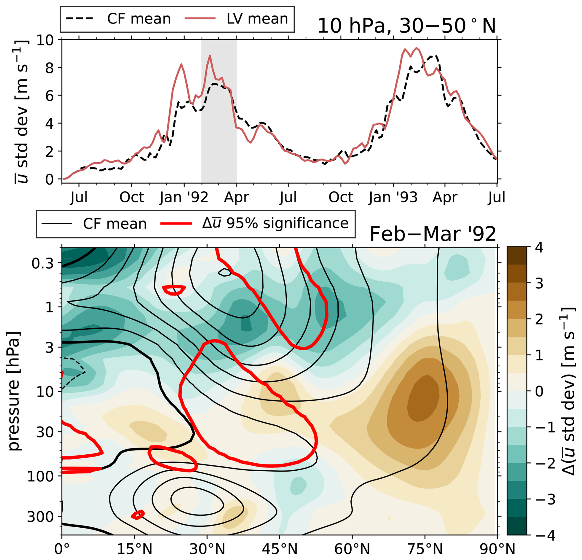
Figure 12 Variability of the polar vortex region in the LV and CF ensembles. Top: standard deviation of $\stackrel{\mathrm{‾}}{u}$ at 10 hPa, averaged from 30 to 50° N, for the LV (red solid) and CF (black dashed) ensemble means. Bottom: the impact (difference between LV and CF ensemble means) of the $\stackrel{\mathrm{‾}}{u}$ standard deviation averaged over February and March 1992, as filled contours (color scale). The time average was chosen to match Fig. 7a and is indicated by a gray band in the top panel. Also plotted is the CF ensemble mean $\stackrel{\mathrm{‾}}{u}$ (black contours), with negative values dashed and the zero line in bold. Solid red contours show the $\mathrm{\Delta }\stackrel{\mathrm{‾}}{u}$ statistical significance (i.e., the bold white contours of Fig. 7a) for reference.

Bittner et al. (2016) state that the reason for the increases of vortex-region variability in their volcanic simulations is unclear. At present, we can only speculate as to the relevant dynamical differences between their model and E3SMv2-SPA. It may be that the QBO is playing a role. Because an easterly QBO phase exists throughout the winter of 1992 in our simulations, we might expect that the vortex should be weakened, and thus destabilized, by the Holton–Tan effect (Holton and Tan, 1980; Lu et al., 2020). However, Fasullo et al. (2024) recently demonstrated that in general, E3SMv2 fails to represent any Holton–Tan-type coupling between the QBO and the extratropics – that is, winter vortex speeds do not decrease relative to a climatological average during easterly QBO states. This not only suggests lesser vortex variability than expected, but it also hints that the background wave activity needs to be fully understood if we are to properly interpret significant post-eruption EP flux anomalies. As the Holton–Tan effect essentially describes QBO-induced changes in Rossby waveguiding in the midlatitudes, it is plausible that the strength (or lack thereof) of the effect could directly interfere with the volcanic aerosol wave-deflection mechanism. A potential avenue for future works is to investigate this interaction more directly, by inspecting, e.g., post-eruption anomalies in potential vorticity and Rossby refraction index distributions. Similar work has recently been done in a stratospheric aerosol injection (SAI) geoengineering context (Karami et al., 2023).

On another note, post-Pinatubo summertime anomalies have received less attention in the literature. In their idealized model studies, DallaSanta et al. (2019) observed that the quiescent summer stratosphere experiences a westerly forcing similar to that of the winter vortex region, which they attribute generically to eddy-driven effects. Toohey et al. (2014) gave more specific consideration to westerly anomalies in the austral summer of 1991 through their simulations with prescribed volcanic forcing. They observed that these anomalies were associated with a statistically significant increase in large-scale wave drag (EPFD) and an accelerated residual circulation (consistent with our Fig. 6), though they did not show how these effects contribute to the TEM momentum budget. Moreover, Bittner et al. (2016) did not analyze summertime anomalies in either hemisphere, and so it has been left unclear whether or not some form of wave-deflection effect acts there as well. Our study has shown that if similar wave driving is present, it does not rise to a level that exerts control over the manifest wind anomalies. Rather, the summertime response is primarily driven by enhanced Coriolis torque due to an acceleration of the advective BDC.

In the tropics, our results read differently than the studies of Brown et al. (2023), though they are not necessarily contradictory. In that paper, the authors describe that the fundamental interaction between volcanic aerosol forcing and the QBO is an increased tropical upwelling, which slows the descent of the coming QBO phase. Our results agree that enhanced diabatic upwelling is the dominant initial response in the tropical region (Fig. 8c), but this does not immediately result in robust impacts on the QBO itself. This is likely because the Pinatubo eruption is offset from the Equator, near 15° N, whereas the aerosol injection used by Brown et al. (2023) was on the Equator. However, by the time significant tropical impacts do arise in our simulations (during boreal spring of 1992) the TEM balance does not indicate that anomalous diabatic vertical motion is responsible. In fact, the weakening of the QBO amplitude and the delay of the westerly phase descent during the boreal summer of 1992 are due largely to increased large-scale and gravity wave drag (Fig. 11).

This apparent contradiction is resolved by the differences in the analysis framework. It must be emphasized that what Brown et al. (2023) call “vertical momentum advection” is specifically $w\times \partial u/\partial z$. This is not the same as $w^{*}\times \partial u/\partial z$; the difference is a contribution of the meridional derivative of the eddy streamfunction ψ (Eq. 10). In other words, an Eulerian-mean upwelling impact Δw evaluated on a pressure-based vertical coordinate will always be some combination of eddy effects and residual-circulation advection from a TEM perspective. Our results indicate that the former can often dominate over the latter in controlling the response of the QBO region. Given the extent of our analysis, we are unable to determine if this conclusion is generic. It may be particular to an easterly-to-westerly QBO transition or to the kind of QBO that exists in E3SMv2 (which, as discussed in Sect. 4.2, is both weak and slow compared to nature). Since the impact significance of the TEM terms is sensitive to the strength of the background, a changing QBO amplitude could change the relative importance of each effect identified by this analysis. It also may be that the conclusion would change for anomalies that occur closer in time to the eruption.

We were not able to test these questions in our current experimental setup, and there is room for future work to further clarify the interaction between the QBO and volcanic TEM anomalies in E3SMv2 or other models. It would be especially useful to perform a resampling analysis on a larger sample size to better understand the robustness of, and the importance of, internal variability in the tropical anomalies.

7 Conclusions

The goal of this study was to use the TEM analysis framework to identify the dynamical processes in control of the development and deterioration of statistically significant zonal-wind anomalies following a large tropical volcanic eruption. The essential result is that, in E3SMv2, while midlatitude westerly anomalies appear consistently for over 1 year in the post-eruption atmosphere, the processes controlling those anomalies are different during the summer and winter. For Pinatubo-sized eruptions occurring during summer in the NH, the initial response is enhanced tropical upwelling, which by mass continuity drives an accelerated BDC and thus increased zonal-wind speeds northward of 30° N (Figs. 6, 8). With these westerly anomalies established, the winter stratosphere is primed for lower-stratosphere equatorward wave deflection, which acts to further intensify upper-level westerly winds in the vortex region (Figs. 6, 7).

The initial upwelling response is as close to a direct aerosol effect that we observed, while the subsequent midlatitude accelerations are indirect consequences of the modified mean meridional circulation and wave propagation. Moreover, the initial upwelling effect does not result in robust wind responses even in the tropical region. Rather, we did not identify significant volcanic impacts on the QBO until the winter of 1992, which were largely wave-driven effects in opposition of the simultaneous QBO phase (Fig. 11).

Our specific conclusions are as follows:

1. We concur with Bittner et al. (2016) that large-scale equatorward wave deflection near the surf zone contributes to post-eruption westerly anomalies in the winter vortex region.

2. We found that the wave-deflection argument only holds in the winter hemisphere. Westerly anomalies in the midlatitude summer stratosphere are instead explained almost entirely by an accelerated residual circulation and thus an anomalous Coriolis forcing of momentum.

3. We observed that a weakened QBO amplitude and a delayed descent of the westerly QBO phase during summer of 1992 were caused primarily by enhanced large-scale and gravity wave drag near 30 hPa. This finding is not necessarily inconsistent with previous studies that instead emphasize the role of perturbed tropical upwelling, as noted in Sect. 6. Effectively, we have identified that the anomalous Eulerian-mean upwelling of momentum affecting the QBO in this context is eddy-driven, rather than simply an enhanced diabatic vertical motion.

4. Practically, we find that regions of robust zonal-wind anomalies can indeed be associated with equally robust forcing anomalies as diagnosed in a TEM framework. However, co-location of these wind and forcing anomalies in space and time is not required; regions where forcing anomalies are insignificant can give rise to significant wind responses, and those responses, once established, may persist after the forcing anomaly ceases.

To our knowledge, this is the only work after Bittner et al. (2016) to demonstrate the wave-deflection pathway in the post-eruption winter stratosphere and the first to provide a full accounting of the TEM momentum balance during specific periods of anomalous stratospheric zonal winds in a volcanic forcing experiment. At this point, we see at least two directions for continued research. As we did not know whether robust wave-driven mechanisms of impact would arise in our simulations, our analysis stopped short of investigating the origin and behavior of the anomalous wave activity in more detail, which could be pursued (see discussion in Sect. 6). In an upcoming work using these same datasets, we will explore the volcanic impacts of the residual streamfunction more directly, as well as the resulting perturbations to stratospheric transit times of trace gases and stratosphere–troposphere mass exchange.

Appendix A: Numerical recipes for tendencies and their integration

The total tendency in the zonal-mean zonal wind ${\stackrel{\mathrm{‾}}{u}}_i$ at time t_i is computed by the first-order accurate forward finite difference

$$\begin{array}{}\text{(A1)}& {\displaystyle \frac{\partial {\stackrel{\mathrm{‾}}{u}}_i}{\partial t}}\approx {\displaystyle \frac{{\stackrel{\mathrm{‾}}{u}}_{i+\mathrm{1}}-{\stackrel{\mathrm{‾}}{u}}_i}{\mathrm{\Delta }t}}\end{array}$$

for an integer $i\in \left[\mathrm{1},N\right]$, where N is the total number of time samples in the dataset, $\mathrm{\Delta }t=(t_{i+\mathrm{1}}-t_i)$, and ${\stackrel{\mathrm{‾}}{u}}_i\equiv \stackrel{\mathrm{‾}}{u}\left(t_i\right)$. Occurrences of Δ in this appendix take the conventional meaning, rather than a notation of impact as in the rest of this paper.

For the analysis presented in Sect. 5, we compute the integrated tendency of a particular component x of the TEM momentum budget (those terms on the right-hand side of Eq. 6) as

$$\begin{array}{}\text{(A2)}& {\stackrel{\mathrm{‾}}{u}}_i^{\left(x\right)}\equiv {\stackrel{\mathrm{‾}}{u}}_n+\mathrm{\Delta }t\sum _{i^{\prime }=n}^i{\displaystyle \frac{\partial {\stackrel{\mathrm{‾}}{u}}_{i^{\prime }}}{\partial t}}{|}_{\left(x\right)}\end{array}$$

for an integer $i\in [n,N]$. This form estimates the total “accumulated” eastward wind speed by the forcing mechanism x over the time period from t_n to t_i, given a common initial condition ${\stackrel{\mathrm{‾}}{u}}_n$. If this recipe is applied to the total tendency $\partial \stackrel{\mathrm{‾}}{u}/\partial t$, then Eq. (A2) is just a reversal of the finite difference procedure Eq. (A1), and the model data ${\stackrel{\mathrm{‾}}{u}}_i$ is recovered exactly. That is, starting the integration from a certain time n does not alter the time series $\stackrel{\mathrm{‾}}{u}$, as expected.

For the TEM components, on the other hand, the choice of n does make a material difference to the time series ${\stackrel{\mathrm{‾}}{u}}^{\left(x\right)}$. This is a important step in the analysis, since there is strong cancellation between the residual circulation and the EP flux divergence forcings, especially in the midlatitudes. There, the net resulting zonal wind is only a relatively small imbalance between these effects. In addition, there is a seasonal asymmetry in the both the residual circulation speed and large-scale wave activity, such that more zonal-wind speed is accumulated by each of these forcing sources during the winter than the summer. Thus, applying Eq. (A2) with n=1 results in two time series $({\stackrel{\mathrm{‾}}{u}}^{\left(v^{*}\right)}+{\stackrel{\mathrm{‾}}{u}}^{\left(w^{*}\right)})$ and ${\stackrel{\mathrm{‾}}{u}}^{(\mathrm{\nabla }\cdot \mathit{F})}$, which simply diverge across the dataset. Choosing n>1 instead calibrates the data to a time period of interest.

In order to apply the significance tests of Sect. 3.1 to the resulting integrated tendencies, Eq. (A2) is computed per ensemble member, for all x and for each unique choice of n. Note that because the unresolved forcing term $\stackrel{\mathrm{‾}}{X}$ (Eq. 18) closes the momentum budget by construction, the sum of ${\stackrel{\mathrm{‾}}{u}}_i^{\left(x\right)}$ over all of the TEM components x also recovers the model data ${\stackrel{\mathrm{‾}}{u}}_i$ exactly.

For the meridional and vertical gradients required for the TEM equations of Sect. 3.2, we use second-order accurate central differences for interior points and either forward or backward finite differences at the boundaries. For a quantity f(ϕ_i), this is

$$\begin{array}{}\text{(A3)}& {\displaystyle \frac{\partial f_i}{\partial \mathit{\varphi }}}\approx \left\{\begin{array}{ll}\frac{f_{i+\mathrm{1}}-f_i}{{\mathit{\varphi }}_{i+\mathrm{1}}-{\mathit{\varphi }}_i}& i=\mathrm{1}\\ \frac{f_{i+\mathrm{1}}-f_{i-\mathrm{1}}}{{\mathit{\varphi }}_{i+\mathrm{1}}-{\mathit{\varphi }}_{i-\mathrm{1}}}& \mathrm{1}<i<N\\ \frac{f_i-f_{i-\mathrm{1}}}{{\mathit{\varphi }}_i-{\mathit{\varphi }}_{i-\mathrm{1}}}& i=N.\end{array}\right.\end{array}$$

An analogous form is used for $\partial f/\partial p$. Note that the TEM equations only require meridional derivatives of zonally averaged quantities. Therefore, the recipe in Eq. (A3) need only be applied to the data after remapping to a uniform latitude grid via Eq. (B9) and is not used on the native grid.

Appendix B: Spherical harmonic zonal averaging

For taking zonal averages, rather than interpolating the data to a latitude–longitude grid, we use a spectral method which allows us to obtain atmospheric variable eddy components on the native cubed-sphere simulation grid. For a 2D scalar A(ϕ,λ), we may write its zonal average $\stackrel{\mathrm{‾}}{A}$ as a superposition of orthonormal basis functions:

$$\begin{array}{}\text{(B1)}& \stackrel{\mathrm{‾}}{A}\left(\mathit{\varphi }\right)=\sum _{l=\mathrm{0}}^{\mathrm{\infty }}{b}_l{Y}_l^{\mathrm{0}}\left(\mathit{\varphi }\right).\end{array}$$

Here, b_l denotes coefficients which scale each contributing basis function, and the basis functions are the set of zonally symmetric spherical harmonics $Y_l^{m=\mathrm{0}}$ of degree l:

$$\begin{array}{}\text{(B2)}& {\displaystyle }{Y}_l^{\mathrm{0}}\left(\mathit{\varphi }\right)=\sqrt{{\displaystyle \frac{\mathrm{2}l+\mathrm{1}}{\mathrm{4}\mathit{\pi }}}}{P}_l\left(\cos \mathit{\varphi }\right),\end{array}$$

where P_l(ϕ) denotes the Legendre polynomials. To justify this definition of $\stackrel{\mathrm{‾}}{A}$, it can be shown that decomposing the dataset A(ϕ,λ) into the full set of spherical harmonics $Y_l^m(\mathit{\varphi },\mathit{\lambda })$ for $\mathrm{0}\le l<\mathrm{\infty }$ and $-l\le m\le l$ and zonally averaging the resulting superposition cause all of the non-symmetric terms (m≠0) to vanish, yielding Eq. (B1).

Computationally, this expression for $\stackrel{\mathrm{‾}}{A}$ can be approximated for a finite set of basis functions on $\mathrm{0}\le l\le L$ as

$$\begin{array}{}\text{(B3)}& \stackrel{\mathrm{‾}}{A}\left(\mathit{\varphi }\right)\approx \sum _{l=\mathrm{0}}^L{b}_l{Y}_l^{\mathrm{0}}\left(\mathit{\varphi }\right).\end{array}$$

Consider a sampling of A resulting in the data vector A defined on a discrete set of N grid points with latitudes ϕ_i. The zonal mean of this data, $\stackrel{\mathrm{‾}}{\mathit{A}}$, is found by solving for the coefficients b_l at each ϕ_i. The spherical harmonic amplitudes for each (ϕ, l) pair are stored in an $N\times (L+\mathrm{1})$ matrix Y₀ and the coefficients b_l in a column vector B:

$$\begin{array}{}\text{(B4)}& \begin{array}{rl}& {\mathbf{Y}}_{\mathrm{0}}=\begin{array}{rc}& \begin{array}{cccc}l=\mathrm{0}& l=\mathrm{1}& \mathrm{\cdots }& l=L\end{array}\\ \begin{array}{c}{\mathit{\varphi }}_{\mathrm{1}}\\ {\mathit{\varphi }}_{\mathrm{2}}\\ \mathrm{⋮}\\ {\mathit{\varphi }}_N\end{array}& \left[\begin{array}{cccc}{Y}_{\mathrm{0}}^{\mathrm{0}}\left({\mathit{\varphi }}_{\mathrm{1}}\right)& Y_{\mathrm{1}}^{\mathrm{0}}\left({\mathit{\varphi }}_{\mathrm{1}}\right)& \mathrm{\cdots }& Y_L^{\mathrm{0}}\left({\mathit{\varphi }}_{\mathrm{1}}\right)\\ Y_{\mathrm{0}}^{\mathrm{0}}\left({\mathit{\varphi }}_{\mathrm{2}}\right)& Y_{\mathrm{1}}^{\mathrm{0}}\left({\mathit{\varphi }}_{\mathrm{2}}\right)& \mathrm{\cdots }& Y_L^{\mathrm{0}}\left({\mathit{\varphi }}_{\mathrm{2}}\right)\\ \mathrm{⋮}& \mathrm{⋮}& \mathrm{\ddots }& \mathrm{⋮}\\ Y_{\mathrm{0}}^{\mathrm{0}}\left({\mathit{\varphi }}_N\right)& Y_{\mathrm{1}}^{\mathrm{0}}\left({\mathit{\varphi }}_N\right)& \mathrm{\cdots }& Y_L^{\mathrm{0}}\left({\mathit{\varphi }}_N\right)\end{array}\right]\end{array},\\ & \mathit{B}=\left[\begin{array}{c}{b}_{\mathrm{0}}\\ b_{\mathrm{1}}\\ \mathrm{⋮}\\ b_L\end{array}\right]\end{array}.\end{array}$$

In matrix notation, Eq. (B3) is

$$\begin{array}{}\text{(B5)}& \stackrel{\mathrm{‾}}{\mathit{A}}\approx {\mathbf{Y}}_{\mathrm{0}}\mathit{B},\end{array}$$

and the coefficients B are solved for by decomposition of the native grid data A onto the zonally symmetric basis set. This requires inversion of Y₀:

$$\begin{array}{}\text{(B6)}& \mathit{B}={\mathbf{Y}}_{\mathrm{0}}^{-\mathrm{1}}\mathit{A},\end{array}$$

and so

$$\begin{array}{}\text{(B7)}& {\displaystyle }\stackrel{\mathrm{‾}}{\mathit{A}}\approx {\mathbf{Y}}_{\mathrm{0}}{\mathbf{Y}}_{\mathrm{0}}^{-\mathrm{1}}\mathit{A}.\end{array}$$

The inversion ${\mathbf{Y}}_{\mathrm{0}}^{-\mathrm{1}}$ can be obtained by computing a least-squares solution to the equation ${\mathbf{Y}}_{\mathrm{0}}^{-\mathrm{1}}{\mathbf{\text{Y}}}_{\mathrm{0}}=\mathbf{\text{I}}$, where I is the (L×L) identity matrix. Alternatively, it can be obtained by ${\mathbf{Y}}_{\mathrm{0}}^{-\mathrm{1}}\equiv {\mathbf{Y}}_{\mathrm{0}}^{\text{T}}\text{diag}\left(\mathit{w}\right)$, where diag(w) is an (N×N) matrix with a vector w of N data weights on the diagonal. The weights provide the areas of the model grid cells, normalized such that the sum of the weights is 4π.

This procedure results in zonal means, and thus eddy components, at all grid points N. Alternatively, an analogous procedure can be followed to recover the zonal mean $\stackrel{\mathrm{‾}}{\mathit{A}}$ on a different, coarser-latitude grid. This is more appropriate for visualization and storage of the zonal-mean components. Given a uniform set of latitudes ϕ^′ of length M≪N, we store the l=0 spherical harmonics at those latitudes in an $M\times (L+\mathrm{1})$ matrix ${\mathbf{Y}}_{\mathrm{0}}^{\prime }$:

$$\begin{array}{}\text{(B8)}& {\mathbf{Y}}_{\mathrm{0}}^{\prime }=\begin{array}{rc}& \begin{array}{cccc}l=\mathrm{0}& l=\mathrm{1}& \mathrm{\cdots }& l=L\end{array}\\ \begin{array}{c}{\mathit{\varphi }}_{\mathrm{1}}^{\prime }\\ {\mathit{\varphi }}_{\mathrm{2}}^{\prime }\\ \mathrm{⋮}\\ {\mathit{\varphi }}_M^{\prime }\end{array}& \left[\begin{array}{cccc}{Y}_{\mathrm{0}}^{\mathrm{0}}\left({\mathit{\varphi }}_{\mathrm{1}}^{\prime }\right)& Y_{\mathrm{1}}^{\mathrm{0}}\left({\mathit{\varphi }}_{\mathrm{1}}^{\prime }\right)& \mathrm{\cdots }& Y_L^{\mathrm{0}}\left({\mathit{\varphi }}_{\mathrm{1}}^{\prime }\right)\\ Y_{\mathrm{0}}^{\mathrm{0}}\left({\mathit{\varphi }}_{\mathrm{2}}^{\prime }\right)& Y_{\mathrm{1}}^{\mathrm{0}}\left({\mathit{\varphi }}_{\mathrm{2}}^{\prime }\right)& \mathrm{\cdots }& Y_L^{\mathrm{0}}\left({\mathit{\varphi }}_{\mathrm{2}}^{\prime }\right)\\ \mathrm{⋮}& \mathrm{⋮}& \mathrm{\ddots }& \mathrm{⋮}\\ Y_{\mathrm{0}}^{\mathrm{0}}\left({\mathit{\varphi }}_M^{\prime }\right)& Y_{\mathrm{1}}^{\mathrm{0}}\left({\mathit{\varphi }}_M^{\prime }\right)& \mathrm{\cdots }& Y_L^{\mathrm{0}}\left({\mathit{\varphi }}_M^{\prime }\right)\end{array}\right]\end{array}\end{array}$$

and the zonal mean of the data is again a composite of these basis functions,

$$\begin{array}{}\text{(B9)}& {\displaystyle }{\stackrel{\mathrm{‾}}{\mathit{A}}}^{\prime }\approx {\mathbf{Y}}_{\mathrm{0}}^{\prime }\mathit{B}={\mathbf{Y}}_{\mathrm{0}}^{\prime }{\mathbf{Y}}_{\mathrm{0}}^{-\mathrm{1}}\mathit{A}.\end{array}$$

This equation transforms the data from a N-point grid in real space to the set of L+1 coefficients b_l in spectral space, before transforming back to an M-point grid in real space.

The matrices Y₀, ${\mathbf{Y}}_{\mathrm{0}}^{-\mathrm{1}}$, and ${\mathbf{Y}}_{\mathrm{0}}^{\prime }$ need only be computed once for a given pairing of computational grid ϕ, remap grid ϕ^′, and choice of L, after which they can be saved to file for use in subsequent computations.

Appendix C: Physically consistent vector-field representation of the meridional circulation

It is common in the literature for authors to visually represent the circulation in the meridional–vertical plane as a vector field with components $(\stackrel{\mathrm{‾}}{v},\stackrel{\mathrm{‾}}{w})$. However, because meridional velocities are typically several orders of larger than vertical velocities, $\stackrel{\mathrm{‾}}{w}$ is often multiplied by a post hoc scaling factor. This scaling factor is usually of order 100, though the specific choice depends on the data localization and processing. In any case, the choice is usually not explicitly justified, and it is often difficult to discern if the direction of the vectors is providing the correct physical picture of the circulation.

Inspired by the scaling recommendations of Jucker (2021) for the EP flux vectors, here we introduce a method of constructing a vector field of the meridional circulation which is physically consistent with rotation in the meridional–vertical plane. Specifically, we define a vector field which, everywhere, is tangent to isolines in a mass streamfunction Ψ (in the form of Eq. 12, with a sign convention such that positive structures in Ψ indicate clockwise rotation, and vice versa). In other words, the curl of the visualized vector field will “look” correct, and regions of zero curl will correspond to Ψ=0. This is usually the implicit goal of manual scaling of the vertical velocity w.

We will assume that the data are provided in a ϕ–p plane, with latitude ϕ in degrees and pressure p in hPa, with p decreasing toward the positive end of the vertical axis. The gradient of Ψ in data units is

$$\begin{array}{}\text{(C1)}& {\displaystyle }\mathrm{\nabla }\mathrm{\Psi }=\left[\begin{array}{c}\partial \mathrm{\Psi }/\partial \mathit{\varphi }\\ \partial \mathrm{\Psi }/\partial p\end{array}\right],\end{array}$$

which we compute by the finite difference methods of Appendix A. With Ψ given in kg s⁻¹, the units of the meridional and vertical components of ∇Ψ are kg s⁻¹ degree⁻¹ and kg s⁻¹ hPa⁻¹, respectively. Because these derivatives are in different units, they must be scaled such that plotting the vector field ∇Ψ shows the correct direction and amplitude at any location in the plot.

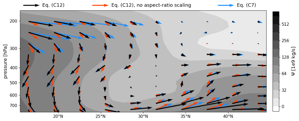
Figure C1 A comparison of three representations of the gradient-normal vector field of a wintertime streamfunction Ψ in the Northern Hemisphere on a log-scaled vertical pressure axis, with a figure aspect ratio of 2.4. Ψ is shown in the grayscale contours. Black arrows show the vectors tangent to isolines in Ψ, as computed by Eq. (C12). Red arrows show the same vectors but with the aspect ratio scaling removed (the horizontal component of Eq. (C12) is multiplied by $\mathrm{\Delta }Y/\mathrm{\Delta }X$). Blue arrows show the vectors as computed by Eq. (C7) without the log-pressure correction. The black arrows are the only ones which are tangent to the Ψ contours everywhere. The blue arrows would be tangent if the vertical pressure axis were linearly scaled. The vector lengths correspond to the magnitude ∇Ψ at each point. The arrows presented in the figure legend represent 4×10¹¹ kg s⁻¹ per unit length of the y axis.

This amounts to a coordinate transformation from data units to “display units”. Following Jucker (2021), we define the display coordinates in the plot as X and Y, respectively, which have units of length (e.g., inches). We also define a pair of normalized coordinates, $x,y\in [\mathrm{0},\mathrm{1}]$, which give the fractional distance along each axis. For any other coordinate $\mathit{\alpha }\in [\mathit{\varphi },X]$ mapping to d≡x, or $\mathit{\alpha }\in [p,Y]$ mapping to d≡y, we use the notation ${\mathit{\alpha }}_{\mathrm{0}}\equiv \mathit{\alpha }(d=\mathrm{0})$, ${\mathit{\alpha }}_{\mathrm{1}}\equiv \mathit{\alpha }(d=\mathrm{1})$, and $\mathrm{\Delta }\mathit{\alpha }\equiv {\mathit{\alpha }}_{\mathrm{1}}-{\mathit{\alpha }}_{\mathrm{0}}$ (occurrences of Δ in this appendix take the conventional meaning, rather than a notation of impact as in the rest of this paper). If the axes are linear, then the data and display units are related by

$$\begin{array}{}\text{(C2)}& {\displaystyle }\mathit{\varphi }\left(X\right)& {\displaystyle }={\displaystyle \frac{\mathrm{\Delta }\mathit{\varphi }}{\mathrm{\Delta }X}}X+{\mathit{\varphi }}_{\mathrm{0}}\text{(C3)}& {\displaystyle }p\left(Y\right)& {\displaystyle }={\displaystyle \frac{\mathrm{\Delta }p}{\mathrm{\Delta }Y}}Y+p_{\mathrm{0}}.\end{array}$$

The streamfunction gradient in the display units is then obtained via the transformations

$$\begin{array}{}\text{(C4)}& {\displaystyle \frac{\partial \mathrm{\Psi }}{\partial X}}& {\displaystyle }={\displaystyle \frac{\partial \mathrm{\Psi }}{\partial \mathit{\varphi }}}{\displaystyle \frac{\partial \mathit{\varphi }}{\partial X}}={\displaystyle \frac{\partial \mathrm{\Psi }}{\partial \mathit{\varphi }}}{\displaystyle \frac{\mathrm{\Delta }\mathit{\varphi }}{\mathrm{\Delta }X}},\text{(C5)}& {\displaystyle \frac{\partial \mathrm{\Psi }}{\partial Y}}& {\displaystyle }={\displaystyle \frac{\partial \mathrm{\Psi }}{\partial p}}{\displaystyle \frac{\partial p}{\partial Y}}={\displaystyle \frac{\partial \mathrm{\Psi }}{\partial p}}{\displaystyle \frac{\mathrm{\Delta }p}{\mathrm{\Delta }Y}}.\end{array}$$

Since we can freely make scaling changes to the components which maintain the vector lengths to a constant factor, we will express this as

$$\begin{array}{}\text{(C6)}& \mathrm{\nabla }{\mathrm{\Psi }}_{(X,Y)}\equiv \left[\begin{array}{c}\mathrm{\Delta }X\times \partial \mathrm{\Psi }/\partial X\\ \mathrm{\Delta }X\times \partial \mathrm{\Psi }/\partial Y\end{array}\right]=\left[\begin{array}{c}\mathrm{\Delta }\mathit{\varphi }\partial \mathrm{\Psi }/\partial \mathit{\varphi }\\ \mathrm{\Delta }p(\mathrm{\Delta }X/\mathrm{\Delta }Y)(\partial \mathrm{\Psi }/\partial p)\end{array}\right],\end{array}$$

where $\mathrm{\Delta }X/\mathrm{\Delta }Y$ is the plot aspect ratio. Finally, we obtain the tangent vector field ∇Ψ^⟂ by swapping the components and applying the desired sign convention:

$$\begin{array}{}\text{(C7)}& {\displaystyle }\mathrm{\nabla }{\mathrm{\Psi }}_{(X,Y)}^{⟂}=\left[\begin{array}{c}-\mathrm{\Delta }p(\mathrm{\Delta }X/\mathrm{\Delta }Y)(\partial \mathrm{\Psi }/\partial p)\\ \mathrm{\Delta }\mathit{\varphi }\partial \mathrm{\Psi }/\partial \mathit{\varphi }\end{array}\right].\end{array}$$

This is the vector field that we plot for visualizing the meridional circulation on linear latitude–pressure axes. Note that if the display coordinates X and Y are expressed in, e.g., inches, then Eqs. (C4) and (C5) have units of kg s⁻¹ in.⁻¹. The components of Eqs. (C6) and (C7) thus have units of kg s⁻¹ y unit⁻¹, where y unit represents a unit length of the y axis, defined by ΔY=1 y unit.

If we are instead visualizing the vector field in a log-pressure vertical coordinate z=log ₁₀(p), then a different transformation for the vertical component is required. If we define a normalized coordinate $y\in [\mathrm{0},\mathrm{1}]$, giving the fractional length along the vertical axis, then the relation between y and p is given by Jucker (2021) as

$$\begin{array}{}\text{(C8)}& {\displaystyle }{\displaystyle }y\left(p\right)={\displaystyle \frac{{\log }_{\mathrm{10}}\left(p_{\mathrm{0}}\right)-{\log }_{\mathrm{10}}\left(p\right)}{{\log }_{\mathrm{10}}\left(p_{\mathrm{0}}\right)-{\log }_{\mathrm{10}}\left(p_{\mathrm{1}}\right)}}={\displaystyle \frac{\ln (p_{\mathrm{0}}/p)}{\ln (p_{\mathrm{0}}/p_{\mathrm{1}})}},\end{array}$$

which implies

$$\begin{array}{}\text{(C9)}& {\displaystyle }p\left(y\right)=p_{\mathrm{0}}{\left(p_{\mathrm{1}}/p_{\mathrm{0}}\right)}^y.\end{array}$$

The derivative of p with respect to the display coordinate Y is then

$$\begin{array}{}\text{(C10)}& {\displaystyle \frac{\partial p}{\partial Y}}={\displaystyle \frac{\partial p}{\partial y}}{\displaystyle \frac{\partial y}{\partial Y}}={\displaystyle \frac{\mathrm{1}}{\mathrm{\Delta }Y}}{\displaystyle \frac{\partial p}{\partial y}},\end{array}$$

and Eq. (C5) is replaced with

$$\begin{array}{}\text{(C11)}& {\displaystyle \frac{\partial \mathrm{\Psi }}{\partial Y}}{\displaystyle }={\displaystyle \frac{\partial \mathrm{\Psi }}{\partial p}}{\displaystyle \frac{\partial p}{\partial Y}}={\displaystyle \frac{\partial \mathrm{\Psi }}{\partial p}}{\displaystyle \frac{\mathrm{1}}{\mathrm{\Delta }Y}}\left(p_{\mathrm{0}}\ln \left({\displaystyle \frac{p_{\mathrm{1}}}{p_{\mathrm{0}}}}\right){\left({\displaystyle \frac{p_{\mathrm{1}}}{p_{\mathrm{0}}}}\right)}^y\right).\end{array}$$

where y in this equation is the evaluation of Eq. (C8) at p. Following the procedure in Eqs. (C6)–(C7) above, the vector field that we plot for visualizing the meridional circulation on latitude–log-pressure axes is thus

$$\begin{array}{}\text{(C12)}& {\displaystyle }\mathrm{\nabla }{\mathrm{\Psi }}_{(X,Y)}^{⟂}=\left[\begin{array}{c}-\frac{\mathrm{\Delta }X}{\mathrm{\Delta }Y}\frac{\partial \mathrm{\Psi }}{\partial p}\left(p_{\mathrm{0}}\ln \left(\frac{p_{\mathrm{1}}}{p_{\mathrm{0}}}\right){\left(\frac{p_{\mathrm{1}}}{p_{\mathrm{0}}}\right)}^y\right)\\ \mathrm{\Delta }\mathit{\varphi }\partial \mathrm{\Psi }/\partial \mathit{\varphi }\end{array}\right].\end{array}$$

Figure C1 shows the effect of these different choices for plotting the gradient-normal vector field of Ψ for a logarithmic vertical pressure axis, with and without the plot aspect ratio scaling and derived log-pressure scaling. This demonstrates that for rendering a vector field parallel to isolines of Ψ while maintaining physically correct vector directions in plots of arbitrary shape, the scalings presented here are the correct ones.