Influence of atmospheric waves and deep convection on water vapour in the equatorial lower stratosphere seen from long-duration balloon measurements

Most atmospheric species enter the stratosphere through the tropical tropopause layer (TTL), a place of interplay between many processes of different scales. Water vapour (H₂O_vap) is a key compound in this layer and its entry into the tropical stratosphere is crucial for stratospheric chemistry and climate. We present a methodology based on the calculation of in situ H₂O_vap and temperature anomalies to estimate the modulation of H₂O_vap due to atmospheric waves and deep convection. H₂O_vap data were obtained from in situ measurements of five Pico-Strat Bi Gaz spectrometers that were flown under long-duration balloons during the Strateole 2 campaigns. The calculation of Pearson's correlation coefficients is performed between averaged ERA5 reanalysis temperatures and in situ H₂O_vap anomalies. In the case of a monotonic vertical gradient of H₂O_vap, the absolute value of the correlation coefficient is high (typically 0.65). For the other flights we highlight lower correlations, due to changes in time of the vertical gradient of stratospheric H₂O_vap, and large convective systems overshooting the tropopause. This is the case for one of the flights, which flew over the Raï typhoon (correlation coefficient of 0.31 due to both contributions). Depending on the flights, we also show that for 47 % up to 70 % of the probed nights, H₂O_vap anomalies can be explained by atmospheric waves, which highlights the major role played by waves on H₂O_vap in the TTL. We also show that long-duration balloon measurements are important in highlighting the overshooting signature of H₂O_vap in the upper TTL.

1 Introduction

Water vapour is the most important greenhouse gas on Earth. In the stratosphere, water vapour plays a major role in the chemical equilibrium, especially in the ozone (O₃) budget, where it is the main source of hydroxyl radical (OH). Furthermore, it plays a significant role in the global radiative budget, especially considering an increase of water vapour during most of the past decades (Solomon et al., 2010; Dessler et al., 2016). Stratospheric water vapour has increased in the middle stratosphere at a rate of 0.5 %–1 % yr⁻¹ (e.g. Oltmans et al., 2000; Rosenlof et al., 2001; Scherer et al., 2008; Hurst et al., 2011) whereas a trend is difficult to estimate near the tropopause due to the variability of its height and the influence of dynamic processes that modulate the abundance of water vapour. Observational studies have shown that the global temperature is sensitive to small changes of water vapour in the lower stratosphere (Forster and Shine, 1999; Solomon et al., 2010; Wang et al., 2017). Aside from transport and modulation processes, stratospheric methane oxidation is the major source of water vapour in the stratosphere (Texier et al., 1988). The observed increase of stratospheric water vapour can be partially explained by the intensification of methane oxidation because of a global increase of methane injected into the stratosphere (Oman et al., 2008; Noël et al., 2018; Tian and Chipperfield, 2006). However, the variability of stratospheric water vapour observed during the 1990s and early 2000s does not follow the increase of methane during the same period (Rinsland et al., 2009; Dlugokencky et al., 2009; Angelbratt et al., 2011). Numerous uncertainties thus remain in understanding the physical, dynamical and chemical mechanisms taking place in the stratosphere that drive the stratospheric water vapour abundance.

The slow ascent above the net zero radiative heating level (14–15 km) in the tropical tropopause layer (TTL) is a major mechanism of water vapour stratospheric variability. During the ascent, air masses first experience decreasing temperatures until reaching the cold point tropopause (CPT). Saturation with respect to ice may be reached, leading to the formation of small ice particles that can sediment and dry the air entering the stratosphere (Gettelman et al., 2000). Therefore, stratospheric water vapour in the tropics is largely linked to the coldest temperature experienced through the slow ascent (the Lagrangian cold point; Fueglistaler et al., 2005). The cold point temperature and height exhibit a seasonal variation as a main driver of stratospheric water vapour variability (Randel and Park, 2019). Deep convection is another important process in the modulation of stratospheric water vapour in the case where it reaches the lower stratosphere (LS) by overshooting convection. Depending on the thermodynamic properties of the LS surrounding the overshoot, these ice particles sublimate and thus hydrate the LS locally (Grosvenor et al., 2007; Chemel et al., 2009; Chaboureau et al., 2007; Frey et al.,2015; Behera et al., 2022). Conversely, if the tropical LS is saturated with respect to ice, particles grow by solid condensation of surrounding water vapour, and sediment if large enough (Hassim and Lane, 2010; Danielsen, 1982). Furthermore, the intensity of deep convection is a determinant factor of the incoming stratospheric water vapour because it modifies the CPT height and, consequently, the TTL temperature (Fueglistaler et al., 2009). The impact of the overshooting deep convection on the stratospheric water vapour budget is not well quantified at the global scale due to the difficulty of considering the variability of the impact of the overshoots at a local scale and having reliable satellite-borne statistics of stratospheric overshoots needed to upscale their impact. Existing climatologies are based on satellite observations, which may miss the peak time of overshooting activity for the continental tropical deep convection (Iwasaki et al., 2010) or the top altitude of the overshoot (which does not necessarily reach the stratosphere, see e.g. Rysman et al., 2017). On the other hand, the convection-permitting simulation of Dauhut and Hohenegger (2022) shows that during the period of 1 August–9 September 2016, deep convection contributed 11 % to the increase in stratospheric water vapour between 10° S and 30° N. Another modelling study suggested that deep convection could contribute on the order of 20 % to 50 % of the increase of stratospheric water vapour at the end of the 21st century (Dessler et al., 2016). In tropical regions, atmospheric waves, usually generated by deep convection, also modulate water vapour: wave-induced temperature perturbations may help to reach saturation with respect to ice. Similarly to the slow ascent in the TTL, ice formation followed by sedimentation can dry the stratosphere. Several modelling studies have investigated the impact of waves on cirrus formation and stratospheric drying (Jensen and Pfister, 2004; Ueyama et al., 2015; Dinh et al., 2016; Podglajen et al., 2016; Corcos et al., 2023; Schoeberl et al., 2019). Waves also indirectly play a role through the Quasi-Biennial Oscillation (QBO). This oscillation is mainly explained by the interaction between Kelvin waves (and to a lesser extent gravity waves) and the mean flow (Dunkerton, 1997). It was shown that during boreal winter between 2015 and 2016 a westerly phase of the QBO and the warm El Niño–Southern Oscillation (ENSO) called El Niño moistened the lower stratosphere with positive anomalies of about 20 % (Diallo et al., 2018).

The interplay between the above-mentioned processes remains a matter of active research. To better understand the couplings, the Strateole 2 project consists of in situ observations near the equatorial tropopause with a suite of instruments flown onboard long-duration super-pressure balloons. In this frame, five Pico-SDLA instruments have been flown (Pico-STRAT Bi Gaz), performing in situ measurements of water vapour, methane and carbon dioxide at a temporal resolution of 4–12 min. The large spatial and temporal extent and high resolution of the measurements open the possibility of linking the observed water vapour variability to the influence of atmospheric waves (of different scales) and deep overshooting convection wherever in the equatorial belt. We rely on calculation of local in situ water vapour anomalies to study the variability of water vapour at different scales.

The paper is organized as follows. Section 2 gives an overview of the Strateole 2 project and of the dynamical context in which the flights took place. Section 3 briefly presents the Pico-STRAT Bi Gaz (hereafter, Pico-STRAT) and Aura MLS (Microwave Limb Sounder) instruments analysed here. Section 4 describes the methodology employed for the analysis with the sensitivity tests specific to each flight. Section 5.1 presents the main results concerning the influence of waves on in situ water vapour. Section 5.2 deals with the signature of deep convection.

2 The Strateole 2 campaigns

Strateole 2 is a project funded by the Centre National d'Etudes Spatiales (CNES, France) and the National Science Foundation (NSF, USA). This project aims at studying dynamical processes in the equatorial lower stratosphere, such as the forcing of the QBO by different types of waves, the formation and life cycle of TTL aerosols and cirrus, as well as the dehydration of the air entering the stratosphere. Another objective is validation of the AEOLUS satellite wind products at the tropics. Strateole 2 relies on three long-duration observation campaigns where a flotilla of super-pressure balloons is launched from Mahé Island in the Seychelles archipelago, in the Indian Ocean off East Africa. Such balloons are nearly Lagrangian platforms carrying scientific instrumentation for flights of several weeks in the TTL and the lower stratosphere (between 18 and 20 km altitude). They evolve on isopycnic surfaces, meaning that the air density remains constant (at first order) during the flight. The first two campaigns took place in 2019/2020 and 2021/2022. A third campaign is planned for 2026/2027. Once afloat, the balloons drift with the wind either eastward or westward depending on the QBO phase.

The balloons can carry up to 15 kg of scientific instrumentation, allowing the probing of several meteorological and chemical variables (wind, pressure, temperature, aerosols, clouds, water vapour, other gases etc.) in situ. Nominal operation of the instruments is ensured by the Zephyr gondola, which is located 1.5 m above Pico-STRAT Bi Gaz on the flight chain. Zephyr is a gondola that provides power (through solar panels), positioning and timing information (onboard GPS receiver) and communication to the ground control centre (using the Iridium space-borne communication system) to the scientific instruments. Some instruments are located inside the Zephyr gondola to protect the electronics from the lower stratosphere cold temperatures (e.g. the thermodynamic sensor, TSEN).

In the frame of this paper we only focus on processes playing a role in the stratospheric water budget. Five Pico-STRATs have already been released during the first two campaigns, allowing the measurement of in situ water vapour, CO₂ and CH₄ mixing ratios. Additional flights of Pico-STRAT Bi Gaz will take place during the last campaign of Strateole 2 at the end of 2026. The trajectories of the flights are shown in Fig. 1.

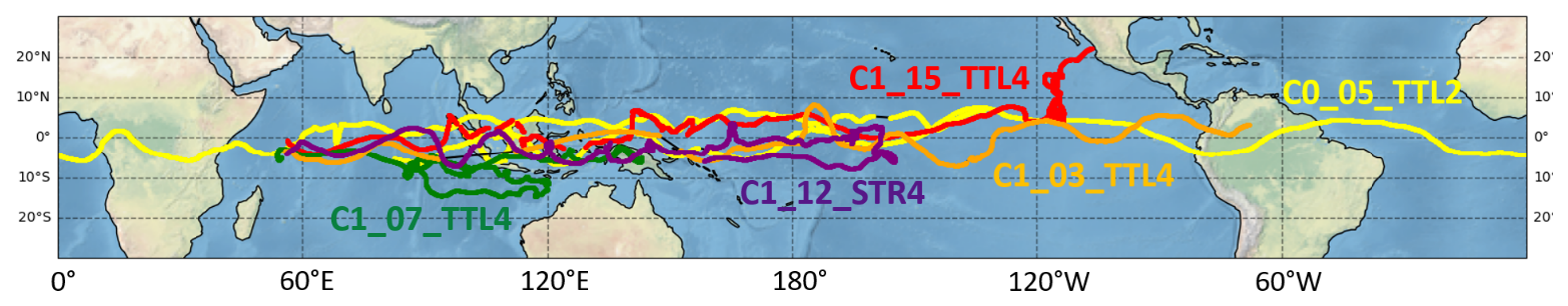
Figure 1 Balloon trajectories of the flights carrying the Pico-STRAT instrument during the first two campaigns. The balloon trajectory in yellow belongs to the first campaign and the others belong to the second campaign.

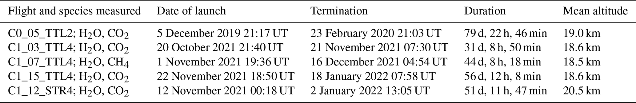
Table 1 lists the flights of Pico-STRAT Bi Gaz during the two Strateole 2 campaigns. In both campaigns the balloon trajectories followed a quasi-zonal eastward propagation within the latitudinal band ±10°. One flight (C0_05_TTL2) measuring water vapour and CO₂ was launched during the first campaign, circumnavigating at the Equator with an average altitude of 19 km. It flew for 79 d within the wet phase of the tape recorder. During the second campaign, three balloons have flown at an average altitude of 18.5 km measuring water vapour and CO₂ (C1_03_TTL4 and C1_15_TTL4) and water vapour and CH₄ (C1_07_TTL4). Another instrument has been flown at an average altitude of 20.5 km, thus above the TTL top altitude, measuring water vapour and CO₂ (C1_12_STR4). The flights lasted between 31 and 56 d, essentially overpassing the Indian and Pacific oceans.

Table 1 Flights of Pico-STRAT Bi Gaz and FLASH-B during the Strateole 2 campaigns in 2019/2020 and 2021/2022.

3 Description of instruments and datasets

3.1 Balloon-borne Pico-STRAT Bi Gaz

Pico-STRAT Bi Gaz is a heritage of the former SDLA (Spectromètre à Diode Laser Accordable; Durry and Megie, 1999), micro-SDLA (Liu et al., 2010) and Pico-SDLA instruments (Ghysels et al., 2011; Ghysels et al., 2012). Pico-STRAT Bi Gaz is a dual-gas tunable-diode laser spectrometer, designed to monitor in situ water vapour, carbon dioxide and methane in the troposphere and stratosphere from large and medium-size open stratospheric balloons, by direct absorption spectroscopy. The general design of the Pico-STRAT Bi Gaz is based on the Pico-SDLA instrument (Durry et al., 2008). Water vapour is probed using an antimonide laser diode emitting at 2.63 µm, while carbon dioxide is probed at 2.68 µm and methane at 3.24 µm. These spectral regions depict strong absorptions within fundamental bands. The strong line intensities of fundamental bands allow a dramatic reduction of the optical path length and thereby make the instruments lighter. Water vapour is probed over a 1 m path length, CO₂ over 50 cm and methane over 2.5 m in ambient air. The diode laser current is modulated to tune the laser frequency, thereby allowing the desired molecular transition to be scanned. The mixing ratio is extracted from the atmospheric absorption spectrum using a non-linear least-squares fitting algorithm applied to the full line shape, based on the Beer–Lambert law and in conjunction with in situ pressure and temperature measurements (Durry and Megie, 1999). The molecular line shape is modelled using a Voigt profile (VP) in the case of water vapour, using line parameters from the HITRAN (high-resolution transmission molecular absorption) database. The CO₂ and CH₄ spectra are modelled using more advanced profiles, fed with laboratory-based line parameters including temperature dependencies (Ghysels et al., 2013, 2014). For CO₂, a Rautian line profile is used while line mixing is added to a Rautian profile in the case of methane. Retrievals are filtered such that the fitting residuals are consistent with the instrument noise.

The in situ spectra are taken at 1 s intervals. During that interval, 200 ms is devoted to recording the elementary atmospheric spectrum (within this time frame, five spectra are recorded), which comprises 256 data points. The remaining 800 ms is used to record the atmospheric pressure and temperature, the GPS data and the status of the instrument (internal temperatures, electronics gains, laser current and temperature, etc.). Pico-STRAT Bi Gaz includes two fast-response Sippican thermistors with an uncertainty of 0.2 °C, located at each end of the optical cell. The air temperature is measured during each acquisition of the in situ atmospheric spectra (every 4–12 min). Each temperature measurement is the average of 20 readings made during 1 ms, with outliers removed. The time between measurements is sufficiently short that successive measurements during a flight differ by less than 0.05 °C. For scientific analysis, the coldest temperature is used.

To suit the Strateole 2-specific operational requirements (instrument weight less than 5 kg, daily power budget limited), the full instrument's electronics, which drives the lasers and acquires the data, is contained in the Zephyr gondola. Doing so allows the electronics to be kept at a safe operating temperature without requiring additional power. The optical cell, including the laser diodes and the detectors, is not located in Zephyr but hangs down, at a 2 m distance, to limit the contamination of water vapour measurements from outgassing Zephyr and balloon surfaces. In this configuration the electronics module is connected to the lasers and the detectors using 2.5 m shielded cables.

3.2 Space-borne Microwave Limb Sounder (MLS)

MLS is an instrument on board the Aura satellite measuring upper tropospheric and lower stratospheric constituents from thermal emission at different bands with a microwave limb sounding system. Water vapour is measured at 190 GHz on 55 pressure levels between 1000 and 0.001 hPa. The vertical grid of water vapour product is 12 levels per decade (LPD) change in pressure for 1000–1 hPa. The water vapour measurement precision, which drives the measurement dispersion, is 7 % at 83 hPa and 6 % at 68 hPa (Livesey et al., 2022). In the present study we use MLS v5 datasets (Livesey et al., 2020). The main differences between MLS v4 and v5 water vapour products are a reduction of an estimated 20 % dry bias below the tropopause (typically 100 hPa), and partial amelioration of a slow positive drift seen in comparisons between MLS and other observations of water vapour in the years since 2010. The extent to which this reduces the drifts reported by Hurst et al. (2016) remains to be investigated. In the present study the MLS v5 water vapour measurements are filtered based on the recommendations in Livesey et al. (2020).

3.3 Himawari-8 Cloud Top Height products (CTH)

Himawari-8 is a new generation of Japanese geostationary meteorological satellite. It was launched in October 2014 by the Japan Meteorological Agency and by the Meteorological Satellite Center (JMA/MSC). Its main instrument is an imager named AHI (Advanced Himawari Imager: Bessho et al., 2016) that consists of 16 channels (3 visible, 3 near-infrared and 10 infrared) with respective resolutions of 0.5, 1 and 2 km, respectively. Cloud Top Height products are deduced with an algorithm adopted by European Organisation for the Exploitation of Meteorological Satellites Nowcasting Satellite Application Facility (EUMETSAT NWC SAF). This algorithm generates CTH products combining data and models. It uses different AHI observations, a radiative transfer model (RTTOV), temperature and humidity vertical profiles (from numerical weather prediction (NWP) models) and cloud-type data deduced from cloud-type and phase products (Kouki et al., 2016). It is applicable for all imagers on board meteorological geostationary satellites and uses the lowest resolution of these imagers. In this study we use CTH products to validate the presence of deep convections that could be linked to water vapour anomalies.

3.4 ERA5 temperature fields

ERA5 is the latest climate reanalysis by ECMWF (European Centre for Medium-Range Weather Forecasts), providing hourly data by combining model data with observations. The ERA5 data are available on a regular latitude–longitude grid at 0.25°×0.25° resolution. The data are given on 37 pressure levels (between 7 and 1000 hPa). Every 12 h, a previous ECMWF forecast is combined with newly available datasets (satellite or in situ observations, including World Meteorological Organization radiosondes) to generate the new estimate of the atmosphere.

ERA5 3D temperature fields are used in the following to build Hovmöller diagrams, which help bring to light the planetary- and large-scale wave activity in the vicinity of the balloon's position. The horizontal resolution of ERA5 temperature fields is 0.25°×0.25° (about 28 km), thus limiting the spectrum of atmospheric waves well resolved by the analysis to horizontal wavelengths greater than ∼300 km at the tropics (Jewtoukoff et al., 2015; Pahlavan et al., 2023; Podglajen et al., 2020; Preusse et al., 2014).

3.5 CALIOP dataset

CALIOP (Cloud-Aerosol Lidar with Orthogonal Polarization) is a space-borne lidar on board the CALIPSO satellite dedicated to cloud and aerosol detection. It can detect the highest cloud layers by backscattering under conditions of a minimum optical thickness of 0.002 at night and 0.001 during daytime. It can also provide information from the inner cloud in cases where the optical thickness is below 3. Measurements are made using two wavelengths (532 and 1064 nm) at an acquisition rate of 20.25 Hz, with a vertical resolution of 30 m between 0 and 40 km and a horizontal resolution of 335 m (Winker et al., 2003, 2009). The CALIOP mission ended in the summer of 2023.

4 Methodology

Figure 2a displays the tape recorder signal over the period December 2018–February 2022, extracted from MLS v5 water vapour products. It shows the alternation of wet and dry phases due to the modulation of the tropopause temperature implying different amounts of water vapour entering the stratosphere and transported upward by the ascending branch of the Brewer–Dobson circulation. The trajectories (time/pressure) of the Pico-STRAT Bi Gaz balloons during the Strateole 2 campaigns are superimposed. Figure 2b and c show zoomed-in views of the first and second campaigns, respectively. All the balloons were flown during the wet phase of the tape recorder. However, it can be noticed that, depending on the balloon flights, the flight occurred during either the drying phase of the wet phase (C0_05_TTL2 and C1_15_TTL4) or during a near steady phase (C1_03_TTL4 and C1_07_TTL4). The balloons have passed over several regions of the Equator for a long time. The in situ time series then depict a background variability which originates from the variability of the tape recorder signal with time and space. Such background must be removed to highlight the modulations of water vapour due to atmospheric waves or overshooting deep convection.

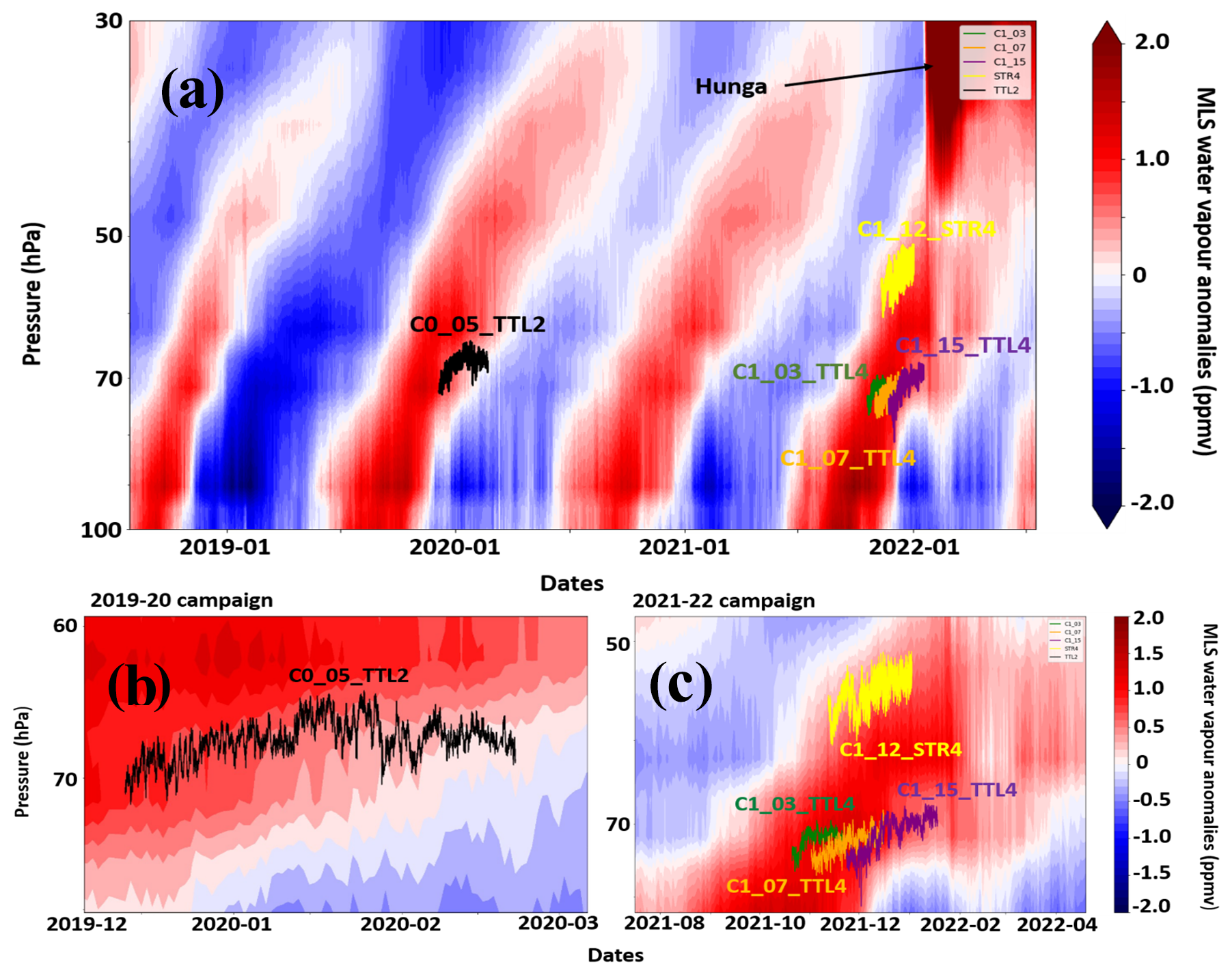
Figure 2 Zonal mean water vapour anomaly of MLS v5 between 10° N and 10° S from July 2018 and July 2022 as a function of air pressure (vertical axis) and time. Panel (a) shows all five flights considered. Panel (b) shows a zoomed-in view of the first campaign period with the trajectory of flight C0_05_TTL2 superimposed. Panel (c) shows a zoomed-in view of the second campaign period with the trajectories of flights C1_03_TTL4, C1_07_TTL4, C1_15_TTL4 and C1_12_STR4 superimposed.

In this section we describe the methodology that permits the removal of this background variability and is used to analyse our water vapour time series.

Such methodology relies on the calculation of in situ anomalies of water vapour (from Pico-STRAT Bi Gaz measurements) relative to a regional mean climatology. The MLS products are used to calculate the mean regional climatology and to estimate the statistics of nights influenced by atmospheric waves. Reanalysis temperatures are used to calculate the Pearson's correlation coefficient of water vapour anomalies, giving an insight on the relative influence of atmospheric waves on the in situ observed anomalies. Section 4.1 summarizes the process in calculating the anomalies, and the data selection and filtering steps preceding the calculation of the anomalies. Section 4.2 and 4.3 are dedicated to the validation of MLS water vapour products and temperature reanalysis (ERA5).

4.1 Data filtering

The methodology we have developed relies on the calculation of local anomalies, which are obtained as the difference between nighttime in situ water vapour measurements and unbiased MLS v5 water vapour values averaged in the same area, around the same date. Since we use two datasets from different instruments, an instrumental bias is expected. This bias must be determined and corrected. In our case, the bias is removed from the MLS dataset. Appendix A.1 gives details of the calculation of the bias and anomalies, as well as the estimation of the anomalies' uncertainties.

Before proceeding with anomaly calculations, the datasets are filtered following quality criteria. First, the Pico-STRAT Bi Gaz data are filtered to remove the effect of water vapour outgassing on the measured mixing ratio. The daytime water vapour data are excluded from the analysis, as well as the first few days of flight. Daytime measurements are contaminated by outgassing of the (tropospheric) water vapour molecules, or supercooled droplets found while crossing high-altitude clouds, which stick to the balloon or the Zephyr surfaces during the ascent of the balloon. As the surrounding pressure decreases, the trapped water is released into the environment, especially during daytime. The nighttime measurements were selected for a threshold solar zenith angle of 95° (measured from the onboard GNSS receiver), which corresponds to a typical sunset at 20 km altitude and for which the measurement dispersion corresponds to the instrumental uncertainty.

In addition to daytime contamination, when comparing in situ nighttime measurements of water vapour with MLS v5 water vapour products the background mixing ratio follows, to some extent, the temporal trend of MLS v5 observations, 5–7 d after the launch. MLS not being affected by outgassing, this comparison demonstrates that nighttime measurements are free from contamination after 5–7 d from launch.

Secondly, the MLS records used in this study are selected following space and time collocation criteria. Regarding the space criterion, we have chosen a circle centred on the position of the balloon at the middle of the night. The circle geometry is independent of the direction of the balloon trajectory and is applicable for any kind of trajectory shape. The circle radius is chosen to be constant for one given flight so that it encompasses for most of the time the distance browsed by the balloon during a single night. The chosen radius is also a compromise between this distance and the total amount of satellite data within the circle, allowing enough data for averaging. This radius scales from 450 to 650 km. The temporal criteria are of major importance since it has the largest impact on the calculation of the anomalies. We have selected the temporal extent so that the impact of large-scale equatorial atmospheric waves is smoothed out. We therefore select 20 d (±10 d around each of the balloon nights), which is longer than the longest wave periods as seen from ECMWF ERA5 reanalysis (fifth generation ECMWF atmospheric reanalysis of the global climate); see also Fathullah et al. (2017).

Finally, the MLS mean value within a circle is interpolated on the mean pressure level of the balloon for a given night. Figure 3 illustrates the results from the selection process for flight C0_05_TTL2, 12–24 December 2019. In Fig. 3a, the two westernmost circles show that the in situ measurements from Pico-STRAT Bi Gaz are wetter than the mean MLS value in the circle, resulting in corresponding wet anomalies for the two corresponding nights, as shown in Fig. 3b.

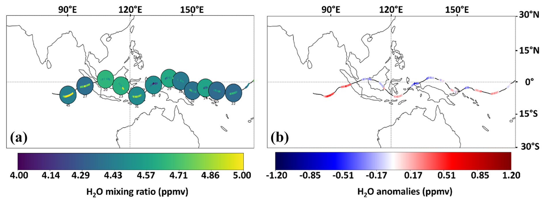
Figure 3 (a) Part of the C0_05_TTL2 night-time trajectory from 12–24 December 2019 with the in situ water vapour measurements colour-coded. The circles show the location of selected MLS v5 water vapour profiles used to calculate a local mean climatology of water vapour ±10 d around each night of the flight. The circles are colour-filled with the mean MLS v5 water vapour mixing ratio. (b) Corresponding anomalies of water vapour as a result of the difference between in situ Pico-STRAT measurements and the local mean MLS v5 value in the circle. The thin black line corresponds to the balloon trajectory during daytime.

4.2 Validation of MLS water vapour profiles and vertical gradient of water vapour

The vertical gradient of water vapour is used to discriminate whether air masses are only vertically displaced under the influence of an atmospheric wave, or if local variations in water vapour are related to direct injections by deep convection. In our study, the vertical gradient of H₂O has been determined from the calculated averaged water vapour profile from MLS v5. In this subsection we compare the in situ Pico-STRAT Bi Gaz vertical profiles, obtained during balloon depressurization events, to the mean calculated MLS profiles to validate the MLS vertical gradient of water vapour.

Depressurization events occur at night when the balloons fly above cold cloud tops (i.e. deep convection), which radiatively cool the helium inside the balloon, reducing the super pressure and inducing a drop in balloon altitude (typically a drop of 800 m to 1.5 km). Once the balloon has passed the convective system, it returns to the initial altitude (following sunrise at the latest). These events provide opportunities to measure the vertical profile of water vapour within the altitude range experienced during depressurization. Figure 4 compares in situ profiles from Pico-STRAT Bi Gaz (green scatter) to MLS profiles (grey lines) ±2 d around three depressurizations. The vertical gradient from the mean MLS profiles (black line) reproduces well the in situ measured vertical gradient (red line). For one case (Fig. 4a, 8 November 2021, 13 November 2021) both in situ and mean MLS profiles capture the inversion of vertical gradient occurring at 82 hPa. Then, the mean MLS profile can be used to calculate the expected sign of the vertical gradient of water vapour in the case of air mass vertically displaced by atmospheric waves. The comparison between the expected sign and the temperature anomaly deduced from ERA5 reanalysis permits determination of whether the observed in situ anomaly is coherent with a vertical displacement. In the following subsection we evaluate the reliability of ERA5 temperature products for such an analysis.

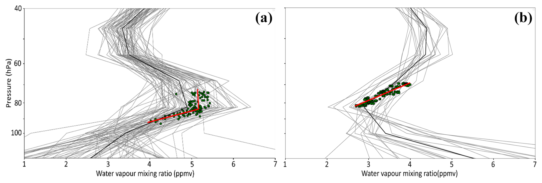
Figure 4 Water vapour vertical profiles of MLS v5 (grey lines) taken ±2 d around the position of depressurization events of Pico-STRAT Bi Gaz (flight C1_07_TTL4 (8 and 13 November 2021) in panel (a) and flight C0_05_TTL2 (28 January 2020) in panel (b)) and the corresponding mean MLS profile (black line). Green scatters are the Pico-STRAT Bi Gaz water vapour profiles obtained during the depressurization (drop and rise). Red lines show the linear interpolation of the Pico-STRAT Bi Gaz profiles.

4.3 Validation of ERA5 temperature products: comparison with in situ balloon-borne measurements

On board each of the balloons, air temperature is measured in situ by two different instruments: Pico-STRAT Bi Gaz and TSEN. Below the Zephyr gondola, the TSEN is a 125 µm-diameter temperature sensor that performs temperature measurements every 30 s. We first compare TSEN and Pico-STRAT Bi Gaz temperatures as a reference comparison – the measurements agree to 0.07±0.41 K and the Pearson's correlation coefficient is 0.82±0.03. Similar agreement is found considering the ECMWF ERA5 temperature field with Pico-STRAT Bi Gaz temperature measurements. The agreement between the Pico-STRAT Bi Gaz measurements and ECMWF ERA5 temperature products is around 0.435±1.38 K, and the Pearson's correlation coefficient is on average 0.74±0.09, close to the in situ comparison. Short-term large deviations can indeed be observed in the case of modulations induced by small-scale atmospheric waves or deep convective events, which are not well resolved in reanalysis. Additionally, some variability in Pearson's correlation coefficient is observed from one flight to another, which relates, to some extent, to the amplitude of the atmospheric waves encountered during the flight. The Pearson's correlation coefficient variability then gives an indirect insight into the dynamics experienced by the instrument, especially in the case of atmospheric wave influence. The ECMWF temperatures therefore compare well with in situ temperatures and can reliably be used for the analysis of wave influence, as proposed in the following.

5 Results and discussion

5.1 Influence of atmospheric waves

In this section we explore the impact of atmospheric waves on the modulation of water vapour by studying the correlation between in situ water vapour anomalies (from Pico-STRAT Bi Gaz measurements) and ERA5 temperature anomalies. ERA5 3D temperature fields are used to build Hovmöller diagrams, which help bring to light the planetary- and large-scale wave activity in the vicinity of the balloon's position. Due to the horizontal and vertical resolution of ERA5 3D fields, the Hovmöller diagram permits identification of waves of wavelengths larger than 300 km. The temperature anomalies (ΔT) are calculated as

$$\begin{array}{}\text{(1)}& \mathrm{\Delta }T=T-\stackrel{\mathrm{‾}}{T},\end{array}$$

where T is the average temperature of ERA5 over ±5° around the mean latitude of the balloon for each night, and $\stackrel{\mathrm{‾}}{T}$ is the zonal mean temperature over the same latitude band.

Then, the ERA5 temperature fields are averaged on the pressure levels encompassed by each balloon. Figure 5 shows longitude/time quasi-Lagrangian Hovmöller diagrams of ERA5 temperature anomalies for the five flights of Strateole 2 carrying the Pico-STRAT Bi Gaz instrument, along with the in situ balloon-borne water vapour anomalies from Pico-STRAT Bi Gaz, which are superimposed on the balloon trajectories. Since the pressure levels of each balloon are different, the pressure range and the latitude range of the averaging in Fig. 5 vary from one flight to another. Figure 5 highlights that temperature perturbations induced by atmospheric waves have an impact on the measured local water vapour anomalies. In some cases, both anomalies obviously evolve in phase over several days (see, for example, panel a).

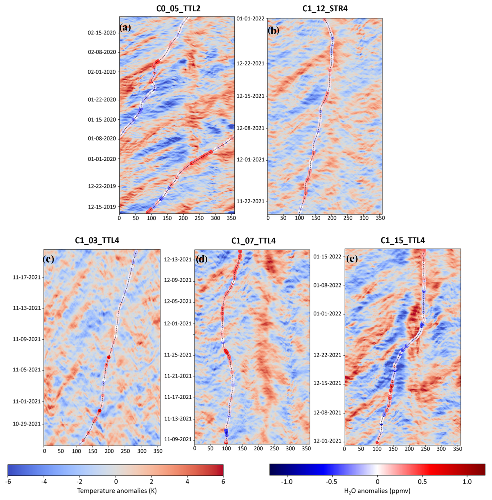
Figure 5 Longitude/time “quasi-Lagrangian” Hovmöller diagrams in temperature anomalies, calculated from ERA5 3D temperature fields for each Pico-STRAT Bi Gaz flight. The balloons' night-time trajectories are colour-coded as a function of balloon-borne water vapour anomalies from Pico-STRAT Bi Gaz. The temperature anomalies are calculated hourly as the difference between the ERA5 temperatures averaged over ±5° around the mean latitude of the balloon for each night and the zonal mean temperature over the same latitude band. (a) C0_05_TTL2 flight. (b) C1_12_STR4 flight. (c) C1_03_TTL4 flight. (d) C1_07_TTL4 flight. (e) C1_15_TTL4 flight.

To estimate the modulation of water vapour due to atmospheric waves, we first calculate the Pearson's correlation coefficient between in situ balloon-borne water vapour anomalies and the corresponding ERA5 temperature anomalies, which are obtained from the “quasi-Lagrangian” Hovmöller diagrams. The following development is aimed at showing that this correlation critically depends on the vertical gradient of the water vapour mixing ratio, which is essentially controlled by the tape recorder signal in the tropical lower stratosphere. Figure 6 shows, with a green line, the wave-induced isopycnic vertical displacement of a super-pressure balloon, and with red dashes the associated isentropic vertical displacement of air masses. The water vapour anomaly measured by the balloon is thus

$$\begin{array}{}\text{(2)}& \begin{array}{rl}{\displaystyle }{X}_b^{\prime }=& {\displaystyle }X\left(A\right)-X\left(B\right)\\ {\displaystyle }=& {\displaystyle }X\left({\stackrel{\mathrm{‾}}{z}}_{\text{balloon}}+{\mathit{\zeta }}_b^{\prime }-{\mathit{\zeta }}_a^{\prime }\right)-X\left({\stackrel{\mathrm{‾}}{z}}_{\text{balloon}}\right),\end{array}\end{array}$$

where X is the water vapour mixing ratio, ${\stackrel{\mathrm{‾}}{z}}_{\text{balloon}}$ is the balloon mean altitude, ${\mathit{\zeta }}_b^{\prime }$ its vertical displacement and ${\mathit{\zeta }}_a^{\prime }$ the wave-induced vertical displacement of the air mass sounded by the balloon (e.g. Fig. 6). If we develop X(A) to the first order, Eq. (2) leads to

$$\begin{array}{}\text{(3)}& \begin{array}{rl}{\displaystyle }{X}_b^{\prime }=& {\displaystyle }X\left(A\right)-X\left(B\right)\\ {\displaystyle }=& {\displaystyle }X\left({\stackrel{\mathrm{‾}}{z}}_{\text{balloon}}\right)+\left({\mathit{\zeta }}_b^{\prime }-{\mathit{\zeta }}_a^{\prime }\right)\times {\displaystyle \frac{\partial \stackrel{\mathrm{‾}}{X}}{\partial z}}-X\left({\stackrel{\mathrm{‾}}{z}}_{\text{balloon}}\right),\end{array}\end{array}$$

where $\partial \stackrel{\mathrm{‾}}{X}/\partial z$ is the background water vapour vertical gradient. According to Podglajen et al. (2014), ${\mathit{\zeta }}_b^{\prime }$ is given by

$$\begin{array}{}\text{(4)}& {\mathit{\zeta }}_b^{\prime }=\mathit{\alpha }\times {\mathit{\zeta }}_a^{\prime }\text{with}\mathit{\alpha }={\displaystyle \frac{g/c_p+\partial \stackrel{\mathrm{‾}}{T}/\partial z}{g/R_a+\partial \stackrel{\mathrm{‾}}{T}/\partial z}}\approx {\displaystyle \frac{\mathrm{1}}{\mathrm{3}}}.\end{array}$$

Hence, the water vapour anomaly becomes

$$\begin{array}{}\text{(5)}& X_b^{\prime }=-(\mathrm{1}-\mathit{\alpha })\times {\displaystyle \frac{\partial \stackrel{\mathrm{‾}}{X}}{\partial z}}\times {\mathit{\zeta }}_a^{\prime }.\end{array}$$

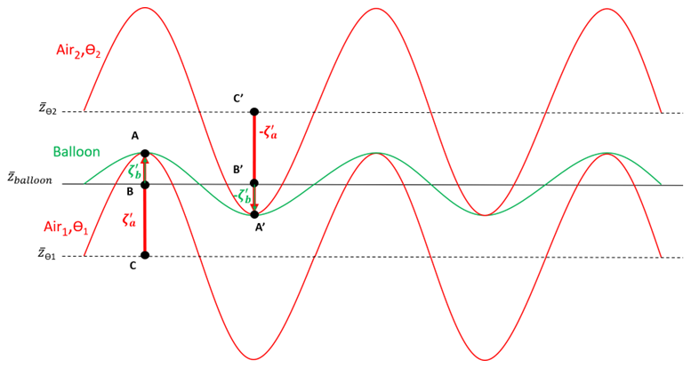
Figure 6 Vertical displacement of the balloon (isopycnic; green line). Vertical displacement of the air masses due to atmospheric waves (isentropic; red lines). The dots C and C^′ are the mean positions of air masses Air₁ and Air₂ at the altitude of the iso-theta 1 and 2 (${\stackrel{\mathrm{‾}}{z}}_{{\mathit{\theta }}_{\mathrm{1}}}$, ${\stackrel{\mathrm{‾}}{z}}_{{\mathit{\theta }}_{\mathrm{2}}}$) without vertical displacements. The dots B and B^′ are the mean positions of the balloon (${\stackrel{\mathrm{‾}}{z}}_{\text{balloon}}$) without vertical displacements. The dots A and A^′ correspond to the air mass sounded by the balloon under the influence of an atmospheric wave. ${\mathit{\zeta }}_a^{\prime }$ and $-{\mathit{\zeta }}_a^{\prime }$ are the upward (from C to A) and downward (from C^′ to A^′) vertical displacements of the air masses Air₁ and Air₂ respectively due to atmospheric waves. ${\mathit{\zeta }}_b^{\prime }$ and $-{\mathit{\zeta }}_b^{\prime }$ are the upward (from B to A) and downward (from B^′ to A^′) vertical displacements of the balloon. The black dashed lines are the mean iso-theta 1 and 2 altitude. The black line corresponds to the balloon mean altitude (${\stackrel{\mathrm{‾}}{z}}_{\text{balloon}}$).

Note that (1−α) is positive in the above equation. On the other hand, the Eulerian wave-induced temperature perturbations estimated in ERA5 are

$$\begin{array}{}\text{(6)}& T^{\prime }\left(A\right)=-\left({\displaystyle \frac{g}{c_p}}+{\displaystyle \frac{\partial T}{\partial z}}\right)\times {\mathit{\zeta }}_a^{\prime }.\end{array}$$

Hence, atmospheric waves are characterized by a correlation between anomalies in balloon-borne water vapour and anomalies in reanalysis temperatures. The sign of this correlation depends on the local vertical gradient of water vapour (hereafter VGWV) at the balloon flight level: it is positive when the vertical gradient is itself positive, and negative otherwise.

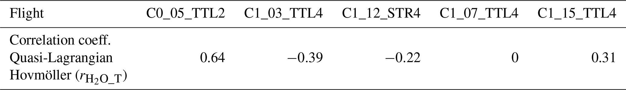
Table 2 lists the Pearson's correlation coefficient ($r_{{\mathrm{H}}_{\mathrm{2}}\mathrm{O}\text{\_T}}$) for each flight. The highest Pearson's correlation coefficient is found for flight C0_05_TTL2 (coefficient: 0.64). For instance, the C0_05_TTL2 flight essentially evolved in a positive vertical gradient of water vapour throughout most of the flight. As such, the C0_05_TTL2 flight can be considered as a reference case, where the influence of atmospheric waves is directly highlighted by the large coefficient. Regarding the other flights, the balloons flew at pressure levels often closer to the inversion of the VGWV (C1_03_TTL4 and C1_07_TTL4) or at a pressure level where the vertical gradient is negative (i.e. flights C1_03_TTL4 and C1_12_STR4), in opposition with flight C0_05_TTL2. Figure 7 shows the calculated MLS water vapour vertical profile over the Maritime Continent covering the period 10–18 December 2021. All the 2021 fights overflew the Maritime Continent, and two of them (C1_07_TTL4 and C1_15_TTL4) overflew it during these 8 d. During this period, the vertical gradient reverses at 69 hPa.

Table 2 Correlation values between “quasi-Lagrangian” Hovmöller temperature anomalies and flight water vapour anomalies.

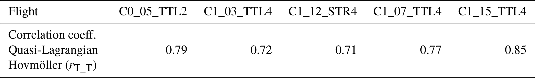
A negative $r_{{\mathrm{H}}_{\mathrm{2}}\mathrm{O}\text{\_T}}$, such as for the C1_03_TTL4 and C1_12_STR4 flights, does not rule out the signature of atmospheric waves in the water vapour modulation. Since atmospheric waves produce temperature anomalies, another way to verify the effective influence of atmospheric waves is to compute the temperature–temperature Pearson's correlation coefficient (r_{T_T}) between ERA5 temperature anomalies and in situ air temperature observed by Pico-STRAT Bi Gaz (see Table 3). The r_{T_T} values listed in Table 3 are high for all the flights: the mean Pearson's correlation coefficient is 0.77±0.06. This indicates that even flights showing near-zero or negative $r_{{\mathrm{H}}_{\mathrm{2}}\mathrm{O}\text{\_T}}$ are strongly influenced by atmospheric waves.

During the period from 28 December 2021 to 9 January 2022, the C1_15_TTL4 balloon flew in a similar structure of the tape recorder as the C0_05_TTL2 balloon (i.e. positive vertical gradient), which has the highest $r_{{\mathrm{H}}_{\mathrm{2}}\mathrm{O}\text{\_T}}$ (0.64). One can thus expect similar Pearson's correlation coefficient for both flights during this period. Indeed, restricting the calculation of the Pearson's correlation coefficient to the period from 28 December 2021 to 9 January 2022 leads to an $r_{{\mathrm{H}}_{\mathrm{2}}\mathrm{O}\text{\_T}}$ of 0.65, very similar to the one obtained for C0_05_TTL2. In both cases, the Pearson's correlation coefficient is therefore in the 0.6–0.7 range, which is the highest value obtained so far for the Strateole 2 flights.

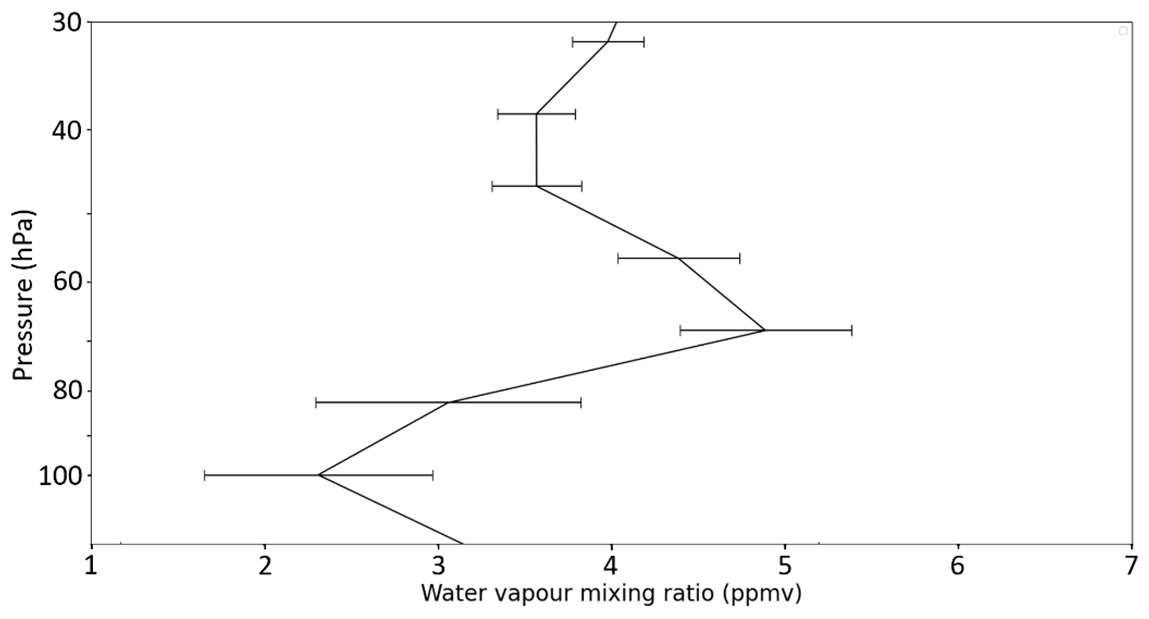
Figure 7 Mean MLS water vapour vertical profile calculated above the Maritime Continent with a time range of 8 d (10–18 December 2021). The error bars show the standard deviation for each pressure level.

Table 3 Correlation coefficient between Hovmöller “quasi-Lagrangian” diagram in temperature anomaly values and in situ temperature of the flight.

Modulations of this Pearson's correlation coefficient can occur when, on some portion of the flight, the balloon evolves at a level close to a vertical gradient reversal or in an altitude range where the vertical gradient of water vapour is small (leading to null correlations). Additional contributions from other short-time or local processes like overshooting deep convection can also be a cause.

A further statistical analysis was performed to estimate the relative contribution of atmospheric waves in the observed water vapour anomalies. By computing the mean Hovmöller temperature anomaly for each night, we can determine whether the balloon is in the presence of a downward (positive temperature anomaly) or upward (negative temperature anomaly) wave-induced vertical displacement. Knowing the actual balloon mean pressure level for the given night and the theoretical vertical displacement, we can then estimate a “theoretical” water vapour anomaly deduced from the mean MLS profile at a given location and time. By comparing the signs of the Hovmöller temperature anomalies and the “theoretical” water vapour anomalies, it is possible to deduce whether the observed balloon-borne water vapour anomalies are consistent with the theoretical vertical displacement.

In the Lagrangian formulation, the wave-induced displacement of air masses are isentropic such that an increase of temperature in the order of 1 K corresponds to a vertical displacement of typically 100 m downward, considering the dry adiabatic lapse rate $-g/c_p=-\mathrm{9.8}\mathrm{K}{\mathrm{km}}^{-\mathrm{1}}$ (note that Eulerian temperature anomalies are actually estimated in ERA5, but the additional $-\partial T/\partial z$ contribution (see Eq. 6) only slightly modifies this estimate). Therefore, the mean Hovmöller temperature perturbation is associated with a “theoretical” vertical displacement. This theoretical displacement allows us to compute the corresponding air mass initial pressure level. To estimate the water vapour anomaly induced by the vertical displacement, we compute a mean MLS vertical profile from MLS water vapour measurements within a 400 km radius and a few days (from 1.5 up to 10 d) around the mean balloon position. The choice of the temporal range for the calculation of the mean MLS profile does not significantly influence the statistics in the range from 1.5 up to 10 d around the mean overnight balloon position: the vertical gradient is nearly constant over this time interval.

The statistics of nights consistent with the theoretical displacement is the largest for flight C0_05_TTL2 (71 % on average), in line with the high correlation coefficient (0.64). The C0_05_TTL2 flight is therefore largely influenced by atmospheric waves. In the case of flight C1_15_TTL4, 60 % of the nights are consistent with the influence of atmospheric waves, though the Pearson's correlation coefficient ($r_{{\mathrm{H}}_{\mathrm{2}}\mathrm{O}\text{\_T}}$) over the whole flight is 0.31. This decrease in Pearson's correlation coefficient is due to the changing dynamics of the tape recorder and to the influence of typhoon Raï (as discussed below). Indeed, the C1_15_TTL4 flight evolved half of the time within each phase of the tape recorder (moistening/drying). while the C0_05_TTL2 flight evolved more than 75 % of the time in the same phase (drying), leading to a strong change in the Pearson's correlation coefficient.

For flights C1_07_TTL4 and C1_03_TTL4, a sensitive difference in the large-scale dynamics led to a smaller number of nights influenced by waves (57 % and 47 %, respectively). For both flights, the correlation coefficient is quite small, with absolute values of Pearson's correlation coefficient lower than 0.4 and night statistics consistently less than 60 %. Flight C1_12_STR4 reaches a ratio of 55 % of nights compatible with vertical displacement of air masses due to waves. Except for C1_03_TTL4, all the flights have more than 50 % of nights compatible with wave activity as seen by water vapour measurements. Overall, these statistics show that during the first two Strateole 2 campaigns, atmospheric waves are an important driver of water vapour modulation.

5.2 Impact of deep convection

The case of flight C1_15_TTL4 brings to light other sources of modulation. From 11–16 December 2021, a large and long-lasting water vapour anomaly (close to 1 ppmv) was detected above Papua New Guinea and the west part of the North Pacific Ocean (see Fig. 5e). In this case, the measurements were influenced by extremely deep convection associated with cyclone Raï. Raï was one of the most intense typhoons of the 2021 season. It started to develop on 8 December 2021, to the northeast of New Guinea, in the Pacific Ocean. It reached Category 1 of the Saffir–Simpson scale on 14 December 2021. On 15–16 December 2021 it reached Category 5 and hit the Philippines. Considering the portions of flight that include the influence of Raï significantly decreases the Pearson's correlation coefficient (down to 0.31, instead of 0.65) when only positive VGWV time periods are considered.

Deep convection can modulate the water vapour in two different ways. Either deep convection brings ice crystals in the lower stratosphere which then sublimate, thereby locally humidifying the stratosphere. Or the air around the convection top is already supersaturated and the injected ice crystals can grow by solid condensation of the ambient water vapour. When large enough, the ice crystals sediment, locally drying the air. Due to the small spatial scale of overshooting tops, the hydration or dehydration signature of overshooting deep convection is expected to be detected over small areas and for short time periods (typically a few hours). Though the balloon is unlikely to have flown exactly at the same time and the same location as an overshoot, it is more likely that the balloons have flown in an air mass that was hydrated or dehydrated earlier by an overshoot.

Another possible signature of deep convection is the vertical displacement of isentropes due to deep convection just below (isentropic levels are moving upward) or upwind (the isentropic levels are moving downwards). This behaviour is highlighted in cloud-resolving model simulations of deep convection (see for example Fig. 9 in Liu et al., 2010). The corresponding signature would be the same as for atmospheric waves without freezing/drying.

Often, before and after a depressurization the water vapour anomalies, whether dry or wet, are large. We thus use here depressurization cases as a proxy of deep convection flyover. Whenever a balloon experiences depressurization during one given night, the water vapour measurements during this given night can potentially be influenced by the deep convective system beneath. Figure 8 shows scatter plots of balloon-borne in situ water vapour anomalies as a function of the potential temperature for the three flights that experienced depressurizations. Please note that the measurements during the balloon depressurizations are not used to compute water vapour anomalies because it would not be possible to compute anomalies associated with a fast variation of altitude. Only data points obtained outside the depressurization for a given day are plotted.

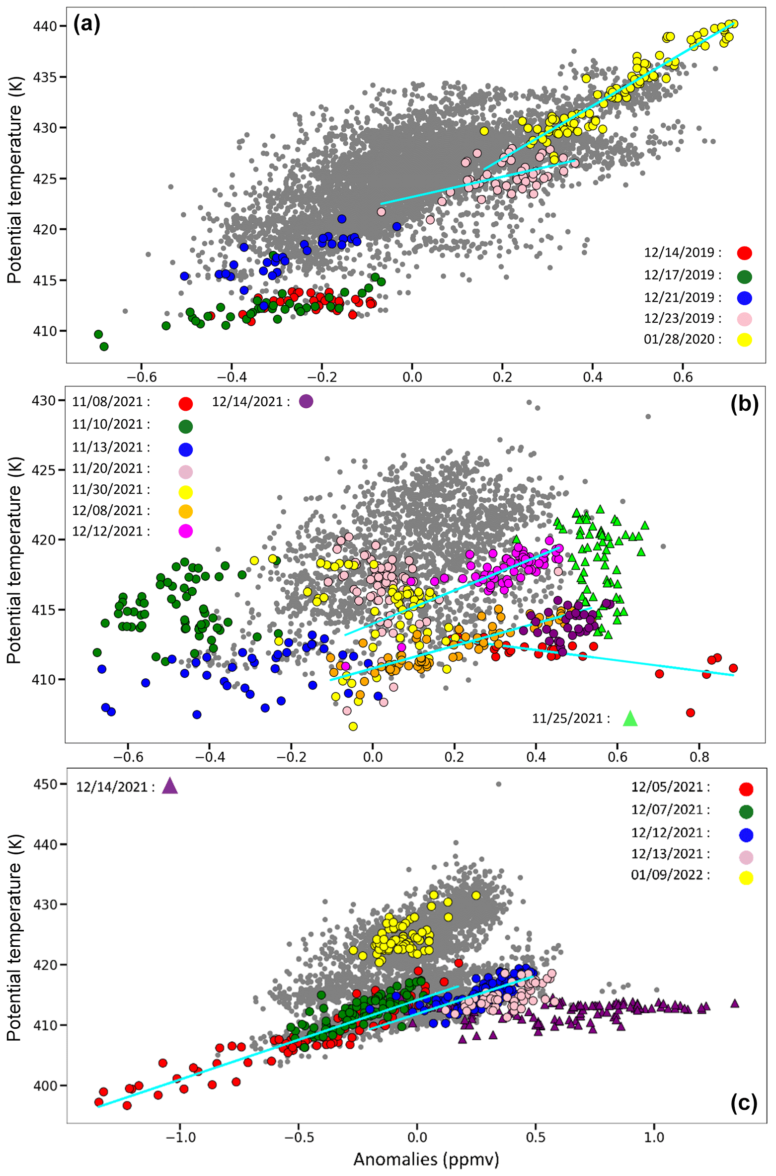
Figure 8 Scatterplot of balloon-borne in situ water vapour anomalies as a function of potential temperature for three flights that experienced depressurizations: (a) C0_05_TTL2, (b) C1_07_TTL4 and (c) C1_15_TTL4. For each panel, cases of depressurization are indicated by a colour code. Dates of depressurization events are given in the legend of each figure. Black dots are for any other dates. For panels (b) and (c), specific coloured triangles are indicated for nights without depressurization but for which deep convection can play a role (see text for details).

Most of the shape of the scatter plots can be explained by the change in time of the tape recorder signal (see Fig. 8).

The C0_05_TTL2 and the C1_07_TTL4 flights exhibit a quasi-linear shape, while the C1_15_TTL4 flight exhibits an S-shape explained by the change in time of the tape recorder state during three different periods of the flight. A contrasting situation is observed for flight C1_07_TTL4, for which the water vapour vertical gradient is much smaller than for flights C0_05_TTL2 and C1_15_TTL4. In this case the repartition of anomalies with potential temperature is significantly different, with an almost absent linear trend.

5.2.1 Vertical displacement of isentropes

Linear behaviour of the balloon-borne water vapour anomalies with potential temperature would indicate that water vapour variations are mainly dominated by the vertical displacement of the balloons. This is due to the vertical gradient of water vapour, as detailed in Sect. 4.1 about the influence of atmospheric waves. On the contrary, injection of ice by overshooting convection followed by sublimation would imply departures of water vapour anomalies from the linear scatter plot. In addition, the freezing/drying mechanism due to waves should also induce a drier signal than the usual linear profile, as well as drying overshooting convection in supersaturated environment.

Looking at nights when the balloons have undoubtedly flown over severe deep convection (that is, depressurization), no systematic signature is found. Some data are especially dry: 14, 17, and 21 December 2019 for C0_05_TTL2; 10 and 13 November 2021 for C1_07_TTL4; 5 December 2021 for C1_15_TTL4. But the observed water vapour anomalies are at least qualitatively consistent with wave activity highlighted in the quasi-Lagrangian Hovmöller diagrams and the mean MLS water vapour profiles. The only exception for the dry cases is the night of 13 November 2021, C1_07_TTL4: the Hovmöller diagram for this night indicates a very weak wave signature (very weak cold temperature anomalies, see Fig. 5d), for which the calculated vertical displacement is too small to explain the amplitude of the dry anomalies. The additional vertical displacement of isentropes due to convection overpassed by the balloon could be an explanation, since upward vertical motion would bring lower mixing ratios from below. Another possible explanation would be the impact of a small-wavelength gravity wave generated by the overpassed deep convective system that is not resolved in ERA5, nor seen in the Hovmöller diagram. The perturbation produced by the gravity wave can accumulate on top of the cold perturbation resolved in the Hovmöller diagram.

Similarly, the case of 5 December 2021, flight C1_15_TTL4, depicts dry water vapour anomalies originating from the cumulative effect of atmospheric waves of different scale. Though very dry, balloon-borne water vapour anomalies remain mostly linear with potential temperature. Such variations might be due to wave activity superimposed on a previous wave-induced dehydration. A radiosonde from Bintulu (west of Borneo Island) indicates saturated layers just above the tropopause at 00:00 UT on 5 December 2021. Though humidity data from radiosondes in this altitude range should be taken cautiously, it indicates a possible supersaturation of the lower stratosphere in the region on the same day. It must be noted that the relative humidity with respect to ice (RHI) computed from the Pico-STRAT Bi Gaz measurements during that night was the highest of all the measurements during Strateole 2 (RHI=91.1 %).

On the other side, several nights with depressurization events are associated with wet anomalies: 23 December 2019 and 28 January 2020, C0_05_TTL2; 8 November 2021, 8 and 14 December 2022, C1_07_TTL4; 12 and 13 December 2021, C1_15_TTL4. For these cases, satellite observations by Himawari show that the balloons were overpassing deep convective systems, while no direct signature of direct injection was observed. Instead, the signatures observed depict a quasi-linear trend with potential temperature, suggesting isentropic displacements, but the amplitude of the anomalies cannot be explained only considering those displacements. These cases represent the limit of our methodology and are not easily interpreted.

In the case of flight C0_05_TTL2 on 28 January 2020 (yellow data in Fig. 8a), the water vapour anomalies follow a linear relation with potential temperature. On the same day, an overpass of CALIOP four hours later and east of the balloon position showed deep convection that overshot the tropopause. Other cloud top products indicated very high convective cells west and four hours earlier than the balloon H₂O maximums. Though the shape of the vapour data on 28 January 2020 are not typical of an overshooting signature, the influence of overshooting deep convection on that day cannot be ruled out and will be the topic of another study.

For the C1_07_TTL4 flight, the wettest dots of 8 November 2021 are discussed in the next section. As for 8 December 2021, though the scatter-plot shape is linear, the wettest dot cannot be compatible with ERA5-resolved wave activity because the Hovmöller temperature anomalies are cold, and the water vapour vertical gradient is such that such a wave pattern should be associated with a dry H₂O anomaly.

For the C1_15_TTL4 flight, all specific depressurization data are compatible with wave- or convective-induced isentropic vertical displacements, except in the case of 12 and 13 December 2021 (see the following discussion). In these cases, the amplitude of the potential temperature displacement (as resolved in ERA5) is small, which suggests that overshooting deep convection could play an important role.

5.2.2 Direct injection

Figure 9 shows four examples of convective cases that might have influenced the water vapour anomalies, and highlights the influence of the Raï tropical storm (which became a cyclone) for two flights. Figure 9 shows cloud top products from the Himawari geostationary satellite with the corresponding balloon trajectories colour-coded with the water vapour anomaly. The time and date of the cloud top image is chosen to be closest to the time when the water vapour anomaly is the highest. Cloud top products are made available by the French AERIS/ICARE (Cloud–Aerosol–Water–Radiation Interactions) data centre. The first two panels of Fig. 9 illustrate the influence of cyclone Raï on 13 and 14 December 2021.

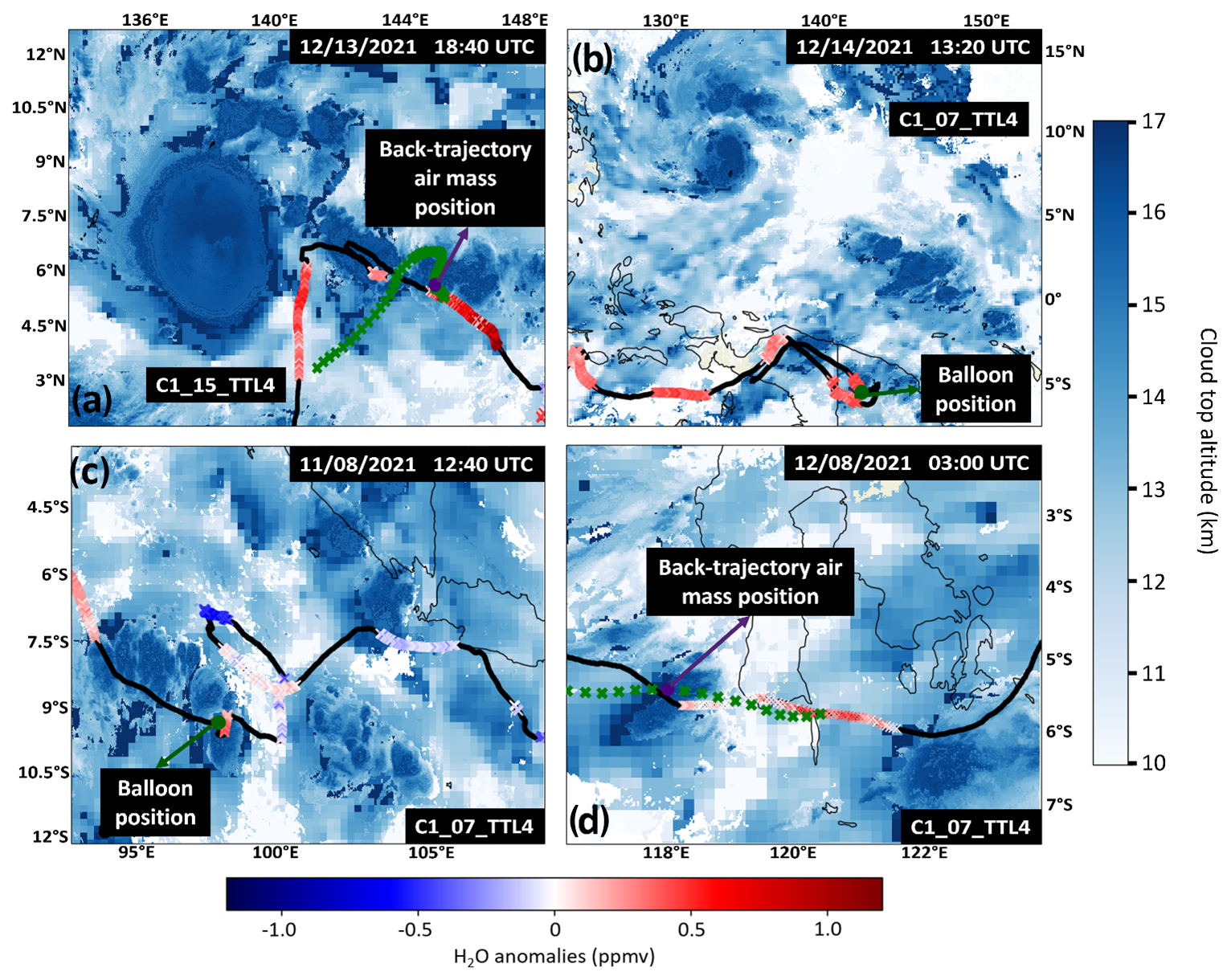
Figure 9 Himawari cloud top products for four convective cases for which specific water vapour anomalies were detected. For each panel, the trajectories of the balloon are superimposed with the corresponding water vapour anomaly (colour coded). The black parts of the balloon trajectory correspond to daytime. (a) 13 December 2021, for the C1_15_TTL4 flight at 18:40 UT. The back trajectory from HYSPLIT initiated from the wettest anomaly position and time is shown with green crosses (one cross every hour). (b) 14 December 2021, for the C1_07_TTL4 flight at 13:20 UT. The green dot is the position of the balloon at that time. (c) As (b) for 8 November 2021, 12:40 UT. (d) 8 December 2021, for the C1_07_TTL4 flight at 03:00 UT. The back trajectory from HYSPLIT initiated from the position and time where the anomaly is the highest is shown with green crosses (one every hour). The position of the air mass at the time of the Himawari image is shown with an indigo dot.

First, the C1_15_TTL4 balloon flew in the vicinity of a spiral rain band of Raï, relatively close to the eye, as shown in Fig. 9a for 13 December 2021 at 18:20 UT. The online Lagrangian model HYSPLIT (Hybrid Single-Particle Lagrangian Integrated Trajectory; Stein et al., 2015; Rolph et al., 2017) was used to compute a back trajectory (green crosses in panel a) initiated from the wettest anomaly position and time (14 December 2021 at 10:00 UT and the position 144.95° E, 5.3° N, 18.6 km altitude). HYSPLIT was run with the GFS (Global Forecast System) analyses. This trajectory shows that the air mass with the wet anomaly, sampled by Pico-STRAT Bi Gaz, was transported through the spiral rain band of Raï a few hours before the measurements. The indigo dot indicates the position of the air mass at the time of the Himawari image. The influence of Raï during this period is undeniable in Fig. 8c for 14 December 2021 (purple triangle) with a signature of quasi-constant potential temperature (413 K) and a local enhancement of water vapour anomaly reaching 1.5 ppmv.

It is worth noticing that the water vapour enhancement of 13 December 2021 in Fig. 8c (pink dots) may also be influenced by Raï, with anomalies above 0.5 ppmv and outside the main scatter plot at 414 K.

The balloon position close to Raï's eye on 12 December 2021 induced a depressurization. Although on the edge of the scatter plot, the water anomaly distribution in Fig. 8c (blue dots) is linear and not typical of an overshoot signature.

The second flight influenced by Raï on 14 December 2021 is C1_07_TTL4. Figure 9b shows part of the balloon trajectory and position (green dot) on 14 December 2021 at 13:20 UT when above New Guinea and the southeastern edge of Raï. The corresponding signature in the water anomaly/theta distribution highlights a few records at 415 K outside the main scatter plot compatible with an overshoot signature, reaching almost 0.6 ppmv of water vapour anomaly. Thus, Strateole 2 is also an opportunity to study the stratospheric hydration associated with tropical cyclones, which will be the topic of a forthcoming publication.

Outside of Raï's influence, the case of 8 November 2021 for C1_07_TTL4 (Fig. 8b, red scatter) departs from the main scatter plot behaviour (reported anomaly around 0.8 ppmv). The Hovmöller diagram in Fig. 5d shows a cold wave perturbation during that night, which should be associated with a dry water vapour anomaly.

Overshooting convection could be a possible explanation for this strong wet signature. Figure 9c shows the trajectory of the C1_07_TT4 balloon on 8 November 2021, with the corresponding water vapour anomalies superimposed on cloud top products from Himawari at 12:40 UT. It shows that on that day, southwest of Sumatra, the balloon flew over a very high convective system reaching at least 16.5 km. The resolution of Himawari (2 km×2 km) is too coarse to detect all the overshooting tops reaching the stratosphere, which are typically at a km² scale. By contrast, the cases situated at the edges of the scatter plots in Fig. 8, and furthermore anti-correlated with what is expected from the quasi-Lagrangian Hovmöller diagram, are limiting cases of the present methodology. A few examples of such cases are summarized below. They could be associated with deep convection of smaller scales compared to the two above-mentioned cases.

Figure 9d illustrates the convective case of 8 December 2021, C1_07_TTL4, when the balloon is south of Sulawesi Island. The corresponding H₂O anomaly / potential temperature scatterplot can be seen in orange in Fig. 8b. During that night, the highest water anomaly reaches 0.53 ppmv, and as stated in Sect. 5.2.1 this behaviour is not compatible with the signature of a wave seen in the Hovmöller diagram. A 3D back trajectory using the online HYSPLIT Lagrangian model, starting from the balloon position where the vapour anomaly is the highest, was computed and is shown with green dots (one dot every hour). It highlights that the air mass sampled by the balloon has overflown a very high convective cell, confirming that deep convection is a plausible explanation for the high water vapour anomaly. The Himawari image time shown in Fig. 9d corresponds to the time at which the back trajectory is above the convective cell (indigo dot at 03:00 UT).

On 25 November 2021 a significant hydration (higher than 0.65 ppmv) at about 420 K is observed (though not during a depressurization night) during the C1_07_TTL4 flight (see Fig. 8b). The calculated vertical gradient of water vapour on that day is insufficient to explain the amplitude of the hydration if it was produced by atmospheric waves. The balloon flew in the vicinity of tropical storm Paddy northeast of Australia, while the storm was dissipating. Paddy was a relatively short-lived storm that formed in the northwest of Australia. It did not reach the typhoon category but impacted Micronesia. The back trajectory calculation did not prove without doubt the overpass of a severe convective cell from Paddy.

To summarize, the isentropic distribution of water vapour anomaly does not always highlight signatures of deep convection, even for nights when depressurization occurred. Some complementary approaches must be developed to separate signals from waves and from deep convection. However, a few cases were highlighted, the most obvious of which is the signature of the Raï cyclone during the C1_15_TTL4 flight and, to a lesser extent, the C1_07_TTL4 flight. This case is associated with stratospheric hydration from 0.6–1.5 ppmv and is a first step to quantifying the impact of tropical cyclones on the stratospheric water budget. Apart from this case, a few convective-compatible signatures of water vapour were underlined with anomalies ranging from 0.4–0.8 ppmv (e.g. C1_07_TTL4 on 8 November 2021 and 8 December 2021), though further analyses are necessary.

6 Summary and conclusion

In 2019–2020 and 2021–2022, in the frame of the first two Strateole 2 campaigns, five Pico-STRAT Bi Gaz instruments were flown from the Seychelles under super-pressure balloons flying at constant density level (between 18 and 20 km) for several weeks in the TTL. The instruments performed in situ measurements of water vapour every 4–12 min during these flights. The present study describes a methodology used to quantify the modulation of water vapour by atmospheric waves and deep convection. This methodology is based on water vapour anomalies calculated from in situ Pico-STRAT Bi Gaz measurements and Aura MLS v5 water vapour products.

The influence of atmospheric waves, like Kelvin waves or gravity waves, has been quantified based on the Pearson's correlation coefficients between ERA5 temperature anomalies and Pico-STRAT Bi Gaz water vapour anomalies. In the cases for which atmospheric waves are the predominant mechanism in the observed modulations of water vapour, the coefficient reaches up to around 0.7 if the vertical gradient of water vapour is large and if the whole flight takes place during a given phase of the tape recorder. This is the case for flight C0_05_TTL2. This flight is a reference case where the tape recorder dynamics produces a positive vertical gradient of water vapour throughout the flight. In this case, atmospheric waves are the predominant factor for the observed modulations, subsequently leading to a high Pearson's correlation coefficient. In other cases, a strongly negative correlation coefficient is obtained when the flight takes place during a negative vertical gradient (flight C1_12_STR4). For the other flights (C1_03_TTL4 and C1_07_TTL4), the balloons evolved during a transition phase of the tape recorder where the vertical gradient reversed, leading to smaller Pearson's correlation coefficients.

The extent to which the Pearson's correlation coefficient is affected by the tape recorder dynamics varies with the stratospheric dynamics experienced by the balloon, though in the case of flight C1_15_TTL4 extremely deep convection from typhoon Raï produced additional modulations of the Pearson's correlation coefficient. In the case that the influence is mixed with deep convection, the Pearson's correlation coefficient decreases to about 0.4 or below. Here, the dynamic of the tape recorder and the associated variability of the water vapour vertical gradient also modulates the Pearson's correlation coefficient throughout the whole flight. We can estimate statistics of the influence of atmospheric waves, considering the vertical structure of the tape recorder. Indeed, flight C0_05_TTL2 is the most influenced by atmospheric waves, with 71 % of the flight consistent with a wave influence, followed by flight C1_15_TTL4 (60 %). Flights C1_07_TTL4 and C1_03_TTL4 depict the same statistics (around 55 %), though in the case of flight C1_07_TTL4 the Pearson's correlation coefficient is close to zero. In such cases, the flight evolved during the steady phase of the tape recorder most of the time. These statistics show that atmospheric waves have a large impact on TTL water vapour, driving the modulation of water vapour during Strateole 2.

Regarding deep convection, our method enables us to discriminate two paths in the modulation of water vapour: direct injection from overshooting tops (large-scale convective system) and vertical displacement of isentropic levels due to deep convection beneath the balloon. In the first case, large convective systems, for which the modulation of water vapour occurs along large distances, have a relatively large impact on the correlation coefficient: this is the case for typhoon Raï (flight C1_15_TTL4) where a 1.5 ppmv enhancement is visible at an almost constant isentropic level. In the case where the observed anomaly is due to a vertical displacement of isentropic level, the repartition of the anomalies follows a quasi-linear trend as a function of potential temperature.

To summarize, this study uses long-duration balloon measurements and an approach based on in situ anomalies of water vapour. We demonstrate that they are useful tools for studying the impact of large-scale waves as well as very intense deep convection on the lower stratospheric water vapour abundance all around the equatorial belt.

Appendix A: MLS H₂O bias estimation and anomaly calculation

Satellite retrievals are based on mathematical processing and physical interpretation of the observed atmospheric radiances. Simplifications and small inaccuracies in the design of the instrument and in the algorithms used to process datasets lead to errors and uncertainties. In the case of MLS v5 H₂O products, the 0.2 %–1 % yr⁻¹ drift identified in v4 products (Hurst et al., 2016) has been partially corrected and, due to the short-term in situ observations, this effect is assumed to be small by comparison with the Pico-STRAT Bi Gaz uncertainty. In addition to the long-term drift of MLS, biases can be observed with in situ measurements. Although the MLS v4 H₂O products have been thoroughly evaluated (Yan et al., 2016; Sheese et al., 2017; Hurst et al., 2016), evaluation of the v5 release needs to be performed. In this section we assess the biases between both Pico-STRAT and MLS v5 H₂O products to build a coherent dataset for our analysis. The full MLS v5 validation study will be the aim of a forthcoming paper.

The temporal coincidence criterion used for assessing the space-borne water vapour bias is a compromise between sufficient closeness in time with the balloon observations and enough MLS data for the statistical analysis. In this line, the temporal criterion is set to ±1 d around the mean overnight balloon position. The spatial criterion is the same as used for the calculation of the anomalies (i.e. 400 km radius around the mean overnight balloon position). The bias is computed as the difference between third-order polynomials fitted on the MLS and Pico-STRAT time series. The resulting bias is then subtracted from the original MLS values (see Fig. A1).

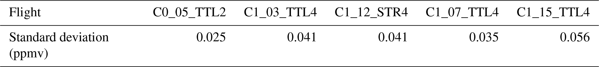
The choice of the space collocation criterion (i.e. the radius circle) has an impact on the representativeness of the calculated bias. In the following we study the influence of the radius on the anomalies reported. First, sensitivity studies show that for circles with a radius ranging from 400–800 km, the mean bias (calculated over ±1 d) remains almost constant, with a variability within 60 ppbv. Therefore, the standard deviation of the water vapour anomalies over one given night should remain almost constant whatever the chosen radius. Figure A2 shows the standard deviation per night for each radius from 400–800 km with a step of 100 km for the C1_07_TTL4 flight. As expected, the standard deviation of the anomalies does not significantly vary for each radius excepted for days 1, 6 and 23. These specific cases can be explained by a local strong variability of MLS water vapour values over ±2 d. Such cases occur for less than 2 % of the total dataset. Secondly, the choice of a given radius may change the calculated anomaly, and potentially its sign, since it considers the variability of water vapour over ±10 d, thereby potentially including the contribution of large-scale dynamics. The variability of the anomaly as a function of the radius is given in Table A1 and permits estimation of the uncertainty of the reported anomalies. The uncertainty of the reported anomalies scales from 0.025 ppmv (for the C0_05_TTL2 flight in 2019–2020) up to 0.055 ppmv (for the C1_15_TTL4 flight). First, the amplitude of the uncertainties remains within the Pico-STRAT Bi Gaz and MLS measurement uncertainty, thereby demonstrating the robustness of the anomaly estimation. Secondly, these uncertainties in the water vapour anomaly are typically one order of magnitude smaller than the anomalies themselves (several tenths of ppmv).

Finally, one can notice that the uncertainty is the lowest for the C0_05_TTL2 flight. Indeed, during this flight the trajectory of the balloon was strongly zonal, remaining within the ±8° latitude range over the whole flight. In such a case the latitudinal variability of water vapour at 18.5 km is low, leading to small variability. In the case of most other flights the latitudinal variability is stronger, so the MLS variability for circles further from the Equator is expected to be stronger.

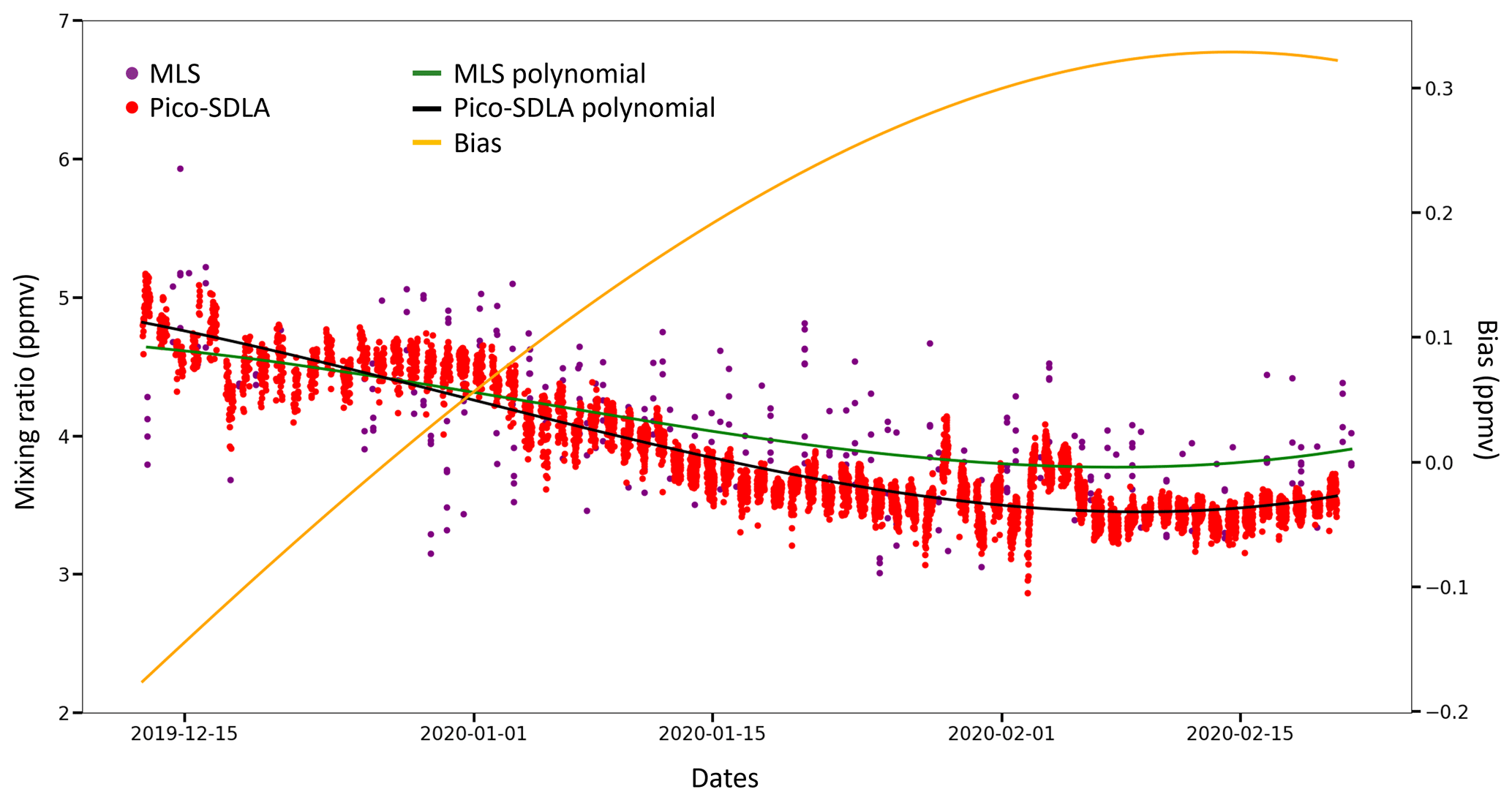
Figure A1 C0_05_TTL2 flight time series of Pico-STRAT Bi Gaz water vapour mixing ratio (red scatters) and MLS v5 (purple scatters) within circles of 400 km radius and ±1 d around a given nighttime. The associated third-order polynomial for Pico-STRAT Bi Gaz is shown in the black line and the MLS polynomial in green. The instrumental bias between MLS and Pico-STRAT Bi Gaz is shown in yellow and is calculated from the difference between the two polynomial fits.

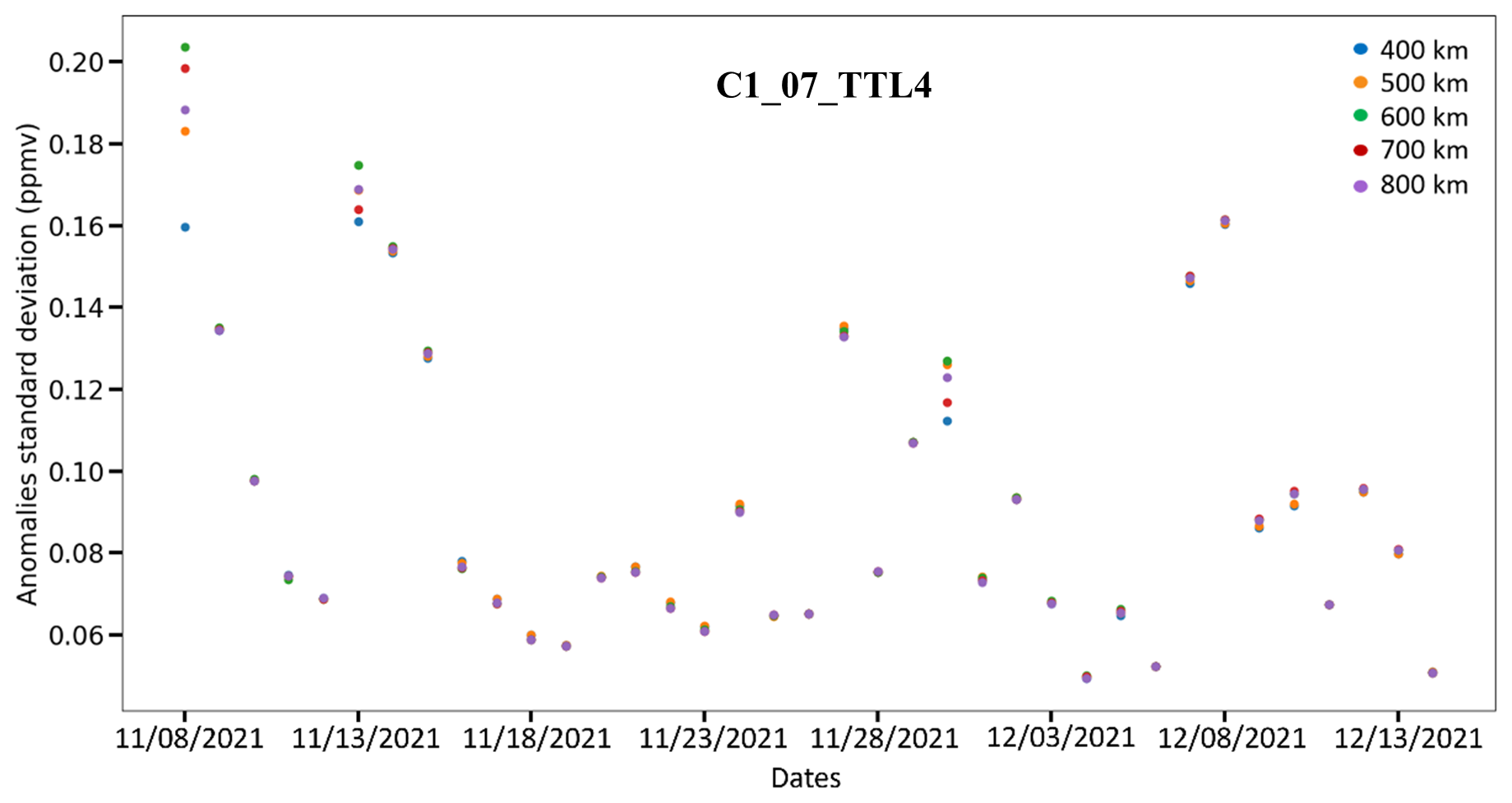
Figure A2 Standard deviation of water vapour anomalies for each night of the C1_07_TTL4 flight, colour-coded as a function of the circle radius used to calculate the anomalies, ranging from 400–800 km with a step of 100 km.

Table A1 Standard deviation of the mean anomalies for varying colocalization radii for each flight.