Factors causing stratocumulus to deviate from subtropical high variability on seasonal to interannual timescales

Stratocumulus (Sc) covers the eastern flanks of maritime subtropical high-pressure systems, and changes in their coverage can exert a radiative effect on the global energy budget comparable to that of a doubling of CO₂. Previous studies have identified the temperature difference between 700 hPa and the surface as the primary driver of Sc variability. However, the mechanistic linkages between subtropical highs and this critical temperature difference, which defines lower-tropospheric stability, remain unresolved. While subsidence modulates temperatures at 700 hPa and wind-driven cooling affects surface temperatures, the observed decoupling between subtropical highs and Sc fraction on seasonal to interannual timescales lacks a mechanical explanation. This study uses reanalysis data to test two hypothesized pathways linking subtropical highs to the lower-tropospheric stability. Results demonstrate that neither pathway dominates, as correlations between Sc-area temperatures and subtropical high dynamics exhibit strong regional and temporal dependencies. Additionally, Sc-area conditions do not systematically align with subtropical high variability, highlighting the need for further investigation into the dynamical processes governing temperatures in the lower troposphere.

1 Introduction

Stratocumulus (Sc), which covers around 20 % of the low-latitude oceans, plays an important role in the global energy budget by reflecting solar radiation (Warren et al., 1986, 1988; Hahn and Warren, 2007; Wood, 2012). Previous studies have verified that changes in its fraction of only 3 %–5 % can lead to effects commensurate with those from a doubling of atmospheric CO₂ concentrations (Hartmann and Short, 1980; Randall and Suarez, 1984; Slingo, 1990), a fact that has motivated a considerable amount of research, including this study, to understand what controls Sc variations and changes.

To understand the variation in Sc, one approach has been to identify and study cloud-controlling factors (Stevens and Brenguier, 2009). Previous researchers have made progressive efforts to define such factors statistically. For instance, already a century ago, it was appreciated that Sc is sensitive to the temperature and humidity difference between the surface and air above the clouds (Blake, 1928). It is now understood that the sensitivity to the temperature difference arises because this difference measures the stability of the Sc–top interface, whereby greater stability suppresses the entrainment velocity, which limits the entrainment drying that inhibits cloud formation. Likewise, for a given entrainment rate, a drier free atmosphere implies more entrainment drying. Klein and Hartmann (1993) made these relationships quantitative by demonstrating a strong and linear relationship between lower-tropospheric stability (LTS), which they defined as the difference between 700 and 1000 hPa, and variations in Sc amount across regions and seasons. Later, Wood and Bretherton (2006) introduced the estimated inversion strength (EIS) to account for differences in lapse rates that influence the relationship between θ at 700 hPa and its more pertinent value, which lies just above the cloud top. They found that EIS explains the variation in low clouds across a wider range of temperature regimes, and hence latitudes, to provide good predictions across tropical, subtropical, and mid-latitude regions. Kawai et al. (2017) combined EIS with the humidity difference into a unified index which they called the estimated cloud top entrainment index (ECTEI). They tested ECTEI using ship observations and found it correlates better with the total low stratiform clouds (including Sc, stratus, and sky-obscuring fog) than EIS. Apart from the role of temperature and humidity differences, a physical understanding of Sc identifies a variety of other physical factors, including large-scale atmospheric subsidence (Weaver and Pearson, 1990; Randall and Suarez, 1984), downwelling longwave radiation above clouds (Stevens and Brenguier, 2009), and sea surface temperature (SST) (Klein et al., 1995).

Based on those factors, and from the spatial coincidence of Sc on the eastern flanks of the semi-permanent subtropical high-pressure regions, an expectation arises that variations in these high-pressure regions will influence Sc. We identify two hypothesized pathways by which the variation in subtropical highs may affect neighbouring regions of Sc. The first hypothesized mechanism is that variations in the subsidence influence the free-tropospheric temperature above Sc, and hence Sc themselves, through enhanced adiabatic warming. If this hypothesis holds, it suggests that variability in Sc may be linked to remote monsoon regions. The pioneering work of Rodwell and Hoskins (1996) has shown a teleconnection between monsoons and subtropical subsidence described as a “monsoon–desert mechanism”. Latent heat release from monsoonal convection generates a westward-propagating Rossby wave that enhances subtropical subsidence, subsequently influencing the free-tropospheric temperature. The second hypothesized mechanism is that variations in the steepness of the high, as measured by the zonal geopotential gradients from its mass centre to the east coast, change surface temperatures through their effect on near-surface winds and the winds' consequent effects on surface currents, ocean upwelling, and surface cooling via wind-driven evaporation. Some evidence for such relationships exists, based on studies that have found Sc to co-vary with the subtropical highs on synoptic (Klein et al., 1995; Klein, 1997; George and Wood, 2010; Toniazzo et al., 2011) and diurnal timescales (Ciesielski et al., 2001; Duynkerke and Teixeira, 2001; Garreaud and Muñoz, 2004). However, these relationships are not particularly strong. Moreover, there is scant evidence for such relationships on seasonal and interannual timescales, in which LTS dominates Sc variation (Klein and Hartmann, 1993; Wood and Bretherton, 2006; Richter and Mechoso, 2004, 2006). A few studies that have addressed this question have found the subtropical highs to be less important than the LTS itself (McCoy et al., 2017; Qu et al., 2015; Zhou et al., 2015). The extent to which this holds up to a more systematic analysis and, if so, whether it is due to confounding influences or simply the fact that the strength of highs is a poor predictor of the constituent terms of cloud-controlling factors, as identified through a statistical analysis, is the focus of the present study. To test the first hypothesized mechanism, we analyse whether subsidence, characterized by ω₇₀₀, warms the free troposphere adiabatically. Similarly, $\frac{\mathrm{d}\mathrm{\Phi }}{\mathrm{d}x}$ represents the steepness of the high in the second hypothesized mechanism, whose changes may influence wind stress, ocean upwelling, and surface temperature. Both factors are selected to describe the features of subtropical highs because they are physically connected to mechanisms proposed to influence EIS. Another commonly used factor for subtropical highs – sea level pressure (SLP) – is found not to be a good representation of either ω₇₀₀ or $\frac{\mathrm{d}\mathrm{\Phi }}{\mathrm{d}x}$ for investigating the mechanical relationship between subtropical highs and EIS.

Specifically, we test the two hypothesized pathways by which the subtropical high-pressure systems may influence cloud amount in the main Sc areas. This requires defining the main Sc areas and the high-pressure areas based on the data, as described in Sect. 2, and identifying whether the quantities hypothesized to be regulated by variations in the subtropical high are indeed the dominant cloud-controlling factors. We first establish a metric for Sc amount (Sect. 2.2) and use this to investigate the contributions of the free-tropospheric and surface pathways to the variation in Sc in Sect. 3.1. Then, the free-tropospheric pathway is tested in Sect. 3.2 and the surface pathway in Sect. 3.3. The investigation of the free-tropospheric pathway follows the logic of how subsidence impacts adiabatic processes (Figs. 4, 5) and hence the potential temperature at 700 hPa (Fig. 6). In addition, the surface pathway is tested through the impact of the geopotential gradient on ocean upwelling and latent heat flux (Fig. 7) and thus changes in the potential temperature at 1000 hPa (Fig. 8). Finally, the correlation between variables in the Sc and subtropical high areas is tested in Sect. 3.4. The conclusions drawn from our analyses are presented in Sect. 4.

2 Data and methods

2.1 Data

This paper uses fifth-generation ECMWF atmospheric reanalysis (ERA5; Hersbach et al., 2017) data for cloud-controlling factors and atmospheric conditions. ERA5 data are provided on a 0.25°×0.25° grid, with three-dimensional fields on 37 pressure levels. The monthly means of SLP, surface latent heat flux, wind components, vertical velocity, temperature, and geopotential heights are analysed.

Low cloud fraction is analysed based on satellite data. This paper uses the second version of the Along-Track Scanning Radiometer and Advanced Along-Track Scanning Radiometer (ATSR-AATSR) data set in the Cloud_cci (European Space Agency Climate Change Initiative) project (Poulsen et al., 2017). The data are provided on a 0.5°×0.5° grid. In this paper, Sc amount is denoted by the symbol κ and defined to be equal to the low cloud fraction (cfc_low) in the identified Sc areas (see Sect. 2.2.1). ATSR-AATSR features a two-view radiometer with seven channels and is one of a number of cloud climatologies that we chose because it is associated with essential climate variables (details are available at https://space.oscar.wmo.int/instruments/view/aatsr, last access: 3 September 2025).

For the ATSR-AATSR data, monthly means for the period from January 2003 to December 2011 are analysed and compared to ERA5 data over the same period. For the analyses of mechanisms that impact the cloud-controlling factors, the 30-year ERA5 record, from January 1985 to December 2014, is analysed. To clarify terminology, our use of the term “seasonal cycle” denotes the monthly climatology, while the term “interannual” denotes the variations in specific monthly values across the record – July for the Northern Hemisphere and January for the Southern Hemisphere. These months are chosen because subtropical highs are at their peak intensity, and Sc reaches its maximum during the summertime, when the monsoon–desert mechanism intensifies subsidence in the vicinity of subtropical highs. We have also examined the interannual variability during the winter season, and the results are consistent with those observed during the summertime period. The “climatological mean” refers to the average over all months for the 30-year record. Hence, for the 30-year ERA5 data, at each spatial location, the seasonal cycle has 12 data points, the interannual record has 30 data point records, and the climatological mean has 1 data point.

2.2 Definitions

A variety of quantities arise in our analysis and are defined as described in the following. In addition to defining the areas over which the analysis is performed and the various cloud-controlling factors being considered, two additional quantities are defined as possible pathways by which the variation in the subtropical highs might influence cloud-controlling factors and hence cloudiness, κ.

2.2.1 Marine subtropical highs and stratocumulus areas

Marine subtropical highs are defined by the union of closed 1020 hPa contours of the climatological mean SLP and marine areas. These are referred to as subtropical high areas (H areas) and are denoted by colours in Fig. 1. Five major regions can be identified across the globe, and these are named the North Pacific (NP), North Atlantic (NA), South Pacific (SP), South Atlantic (SA), and South Indian (SI) oceans.

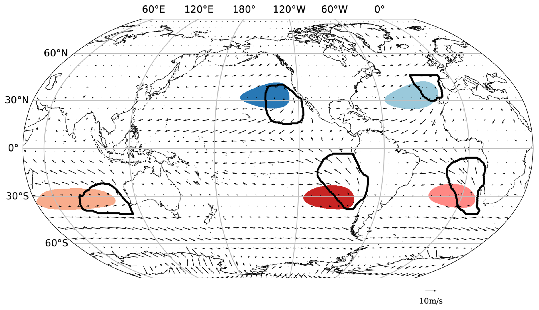
Figure 1 The defined H areas (shaded) and c areas (thick black lines). The arrows denote a 10 m wind field. Each colour represents one region, and it is consistent in the later analyses. The map uses the Robinson projection.

Similarly, Sc areas (c areas) are defined when the mean low cloud fraction of 9 years is greater than 0.5 (or 0.4 for NA) and falls within 45° N–45° S. These c areas are shown as thick black contours in Fig. 1. Figure 1 shows that the c areas are typically located eastward of H areas.

This paper uses similar words to address different concepts. “Regions” specifies the difference between NP, NA, SI, SP, and SA. “Areas” specifies the difference between H and c areas. Subscripts “H” and “c” represent the area over which the variables are averaged.

2.2.2 Cloud-controlling factors

Previous studies have suggested four factors to represent lower-tropospheric conditions: the hydro-lapse (ℋ), LTS, EIS, and ECTEI (Klein and Hartmann, 1993; Wood and Bretherton, 2006; Kawai et al., 2017), as defined below:

ℋ.

The hydro-lapse is defined as

$$\begin{array}{}\text{(1)}& \mathcal{H}=\mathit{\beta }{\displaystyle \frac{l_{\mathrm{v}}}{c_{\mathrm{p}}}}(q_{\mathrm{700}}-q_{\mathrm{1000}}),\end{array}$$

where β=0.23, l_v is the latent heat of vaporization, c_p is the specific heat of air at constant pressure, and q is the specific humidity. Here and throughout, a numeric subscript denotes the pressure level in units of hPa.

LTS.

The lower-tropospheric stability is defined as

$$\begin{array}{}\text{(2)}& \mathrm{LTS}={\mathit{\theta }}_{\mathrm{700}}-{\mathit{\theta }}_{\mathrm{1000}},\end{array}$$

where θ is the potential temperature.

EIS.

The estimated inversion strength is defined as

$$\begin{array}{}\text{(3)}& \mathrm{EIS}=\mathrm{LTS}-{\mathrm{\Gamma }}_{\mathrm{850}}\left(Z_{\mathrm{700}}-\mathrm{LCL}\right),\end{array}$$

where Γ denotes the moist lapse rate, and Γ₈₅₀ is calculated by the average temperature of 700 and 1000 hPa. Z denotes the geopotential height. LCL is the lifting condensation level. To estimate the LCL, we assume a constant surface relative humidity of 80 %, consistent with that of Wood and Bretherton (2006). Based on the approximations $\mathrm{RH}\approx \mathrm{100}-\mathrm{5}(T-T_{\mathrm{d}})$ and $\mathrm{LCL}\approx \mathrm{125}(T-T_{\mathrm{d}})$ with RH in %, LCL in m, and T and T_d in K, from Lawrence (2005), the difference between surface temperature and dew point is approximately 4 K, and the corresponding LCL is about 500 m.

ECTEI.

The estimated cloud top entrainment index is defined as

$$\begin{array}{}\text{(4)}& \mathrm{ECTEI}=\mathrm{EIS}+\mathcal{H}.\end{array}$$

Some recent studies have re-evaluated LTS and EIS and have found that they have little difference in their ability to describe cloud amounts and that this difference varies with data sources (Cutler et al., 2022; Park and Shin, 2019). For this reason we re-examine the correlation between each suggested factor and κ to select the one that is the best predictor. Figure 2 shows that EIS best explains variations in κ across all monthly means. Analyses of the same correlations on both the seasonal (r=0.93) and the interannual (r=0.79) timescales are consistent with the results based on all monthly means. Hence, EIS is selected for the following investigation. The performance of ℋ is the worst. Even though ℋ and κ are correlated at least in SP and SA, in these regions the correlations are also weaker than those between κ and the other factors. This agrees with Klein and Hartmann (1993), who claim that moisture dominates changes in stratus in the Arctic but not in subtropical Sc. For this reason (which we also confirm through a supplementary analysis but do not include here), the effects of subtropical highs on Sc through the influence of their variations on free-tropospheric humidity are not explored further.

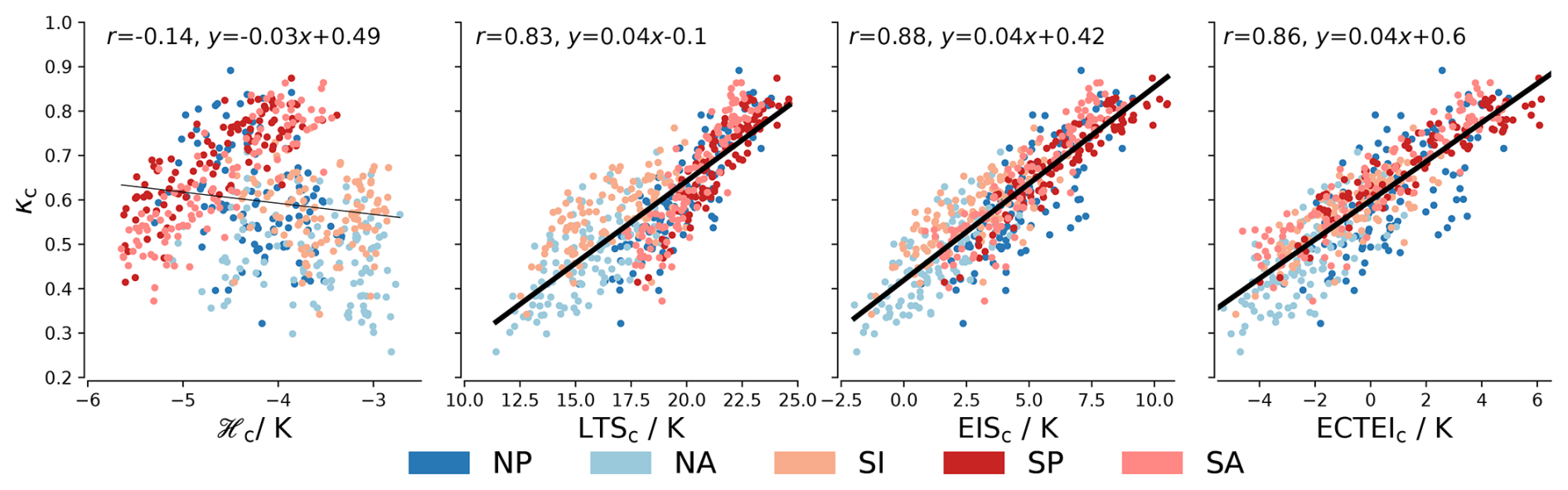
Figure 2 Scatter plots of different cloud-controlling factors and low cloud fraction (κ) from 2003 to 2011. Each scatter point represents a monthly mean, and the plots include 9 years of data, covering all 12 months per year. From left to right: the cloud-controlling factors are ℋ, LTS, EIS, and ECTEI, analysed over the cloud (c) areas, as denoted by the subscripts. All subplots share the same y axis, which represents κ, with each plot displaying data points coloured by different regions. Regression lines are presented for p values ≤ 0.05 and are thicker when r²≥0.25.

2.2.3 Adiabatic warming of lower free troposphere

For a stronger high-pressure system, we expect greater subsidence and more adiabatic warming, which in the mean would need to be balanced by increased radiative cooling or advection.

To explore the link between the lower-tropospheric potential temperature and the high-pressure regions, we look toward the thermodynamic energy equation. Assuming stationarity, adiabatic warming (Q) must be balanced by diabatic warming/cooling (Q_Diab) such that

$$\begin{array}{}\text{(5)}& Q=-Q_{\mathrm{Diab}}=-(\mathit{v}\cdot \mathrm{\nabla }\mathit{\theta }+\mathit{\omega }{\displaystyle \frac{\partial \mathit{\theta }}{\partial p}}).\end{array}$$

Here v⋅∇θ denotes horizontal advection, with v being the horizontal wind vector, and $\mathit{\omega }\frac{\partial \mathit{\theta }}{\partial p}$ describes vertical advection, with ω representing vertical (pressure) velocity and p denoting pressure. Q_Diab can be associated with the convergence of radiant energy or with turbulent mixing caused by co-variances arising from the use of mean quantities in forming the budget terms.

2.2.4 Wind-driven surface cooling

According to our second hypothesis, a high-pressure system with a larger zonal geopotential gradient ($\frac{\mathrm{d}\mathrm{\Phi }}{\mathrm{d}x}$) would be accompanied by a cooler surface. This could be due to a variety of mechanisms. First, it leads to more equatorward winds due to the geostrophic balance:

$$\begin{array}{}\text{(6)}& v={\displaystyle \frac{\mathrm{1}}{f}}{\displaystyle \frac{\mathrm{d}\mathrm{\Phi }}{\mathrm{d}x}},\end{array}$$

where v is the meridional wind component, Φ is the geopotential, x represents distance in the zonal direction, f is the Coriolis parameter, and we analyse $\frac{\mathrm{d}\mathrm{\Phi }}{\mathrm{d}x}$ at 700 hPa.

The consequently increased surface wind stress leads to more ocean upwelling and hence surface cooling. This upwelling is measured by the Ekman pumping velocity, w_E:

$$\begin{array}{}\text{(7)}& w_{\mathrm{E}}=\mathrm{\nabla }\times \left({\displaystyle \frac{\mathit{\tau }}{{\mathit{\rho }}_{\mathrm{0}}f}}\right).\end{array}$$

Here ${\mathit{\rho }}_{\mathrm{0}}=\mathrm{1030}\mathrm{kg}{\mathrm{m}}^{-\mathrm{3}}$ is the density of ocean water, and

$$\begin{array}{}\text{(8)}& \mathit{\tau }={\mathit{v}}_{\mathrm{10}}\cdot {\mathit{\rho }}_{\mathrm{a}}{C}_{\mathrm{D}}\Vert V\Vert \end{array}$$

is the surface wind stress, with ${\mathit{\rho }}_{\mathrm{a}}=\mathrm{1.225}\mathrm{kg}{\mathrm{m}}^{-\mathrm{3}}$ being the density of near-surface air, C_D denoting the drag coefficient, v₁₀ representing the near-surface (10 m) horizontal wind, and $\Vert V\Vert$ being the near-surface wind speed. Since wind speeds are moderate in subtropical high and Sc regions, the drag coefficient C_D is assumed to be constant at 0.0012, following Large and Pond (1981). A positive value of w_E means upwelling motion, and a negative value means downwelling motion. Unlike other variables, w_E is analysed in a continuous area of positive w_E near the coast.

In addition, increased surface winds can also cool the surface through enhanced evaporation, which is measured by the latent heat flux (LHF).

3 Analysis

In this section we first explore what factors explain variations in EIS, which we now use as a proxy for cloudiness (κ). We then explain to what extent these factors can be related to variations in the subtropical high-pressure regions.

3.1 Dependence of EIS on θ₇₀₀ and θ₁₀₀₀

EIS differs from LTS as it includes the temperature-dependent lapse rate Γ, but it is dominated by the variations in LTS (i.e. the difference between θ₇₀₀ and θ₁₀₀₀) because any change in lapse rates depends on the change in the temperature below 700 hPa. Table 1 shows how these quantities vary across different regions and for different timescales and how much they contribute to variability in EIS.

In the higher-latitude regions of the NP, NA, and SI, variations in θ₇₀₀ are mostly larger than variations in θ₁₀₀₀ in both the seasonal and the interannual data, and they explain a large part of the variability in EIS in those regions, particularly on seasonal timescales. In these regions, θ₇₀₀ and θ₁₀₀₀ strongly co-vary across the seasonal cycle, but θ₇₀₀ varies more. This means that EIS increases even as θ₁₀₀₀ increases, which explains the otherwise counterintuitive positive correlation between θ₁₀₀₀ and EIS in the higher-latitude regions on seasonal timescales. For the more equatorward regions of the SP and SA, variability of EIS is dominated by θ₁₀₀₀, of which the variability is much larger than that of θ₇₀₀ on seasonal timescales. This result is consistent with that of Klein and Hartmann (1993), who found that lower-tropospheric stability co-varies with θ₇₀₀ in NP, NA, and SI and with SST in other regions. Moreover, variations in θ₁₀₀₀ are important for all regions on interannual timescales (as evidenced by the correlations between θ₁₀₀₀ and EIS in Table 1) and are particularly important for the main Sc areas of the NP and SA, as well as for the SI, where the standard deviations of θ₁₀₀₀ and θ₇₀₀ are nearly equal.

Table 1 Correlation (r) with EIS and standard deviation (σ) for the quantities θ_1000c, θ_700c, and ω_700H over the seasonal cycle and the interannual variability. The level with a higher correlation is denoted by the bold font.

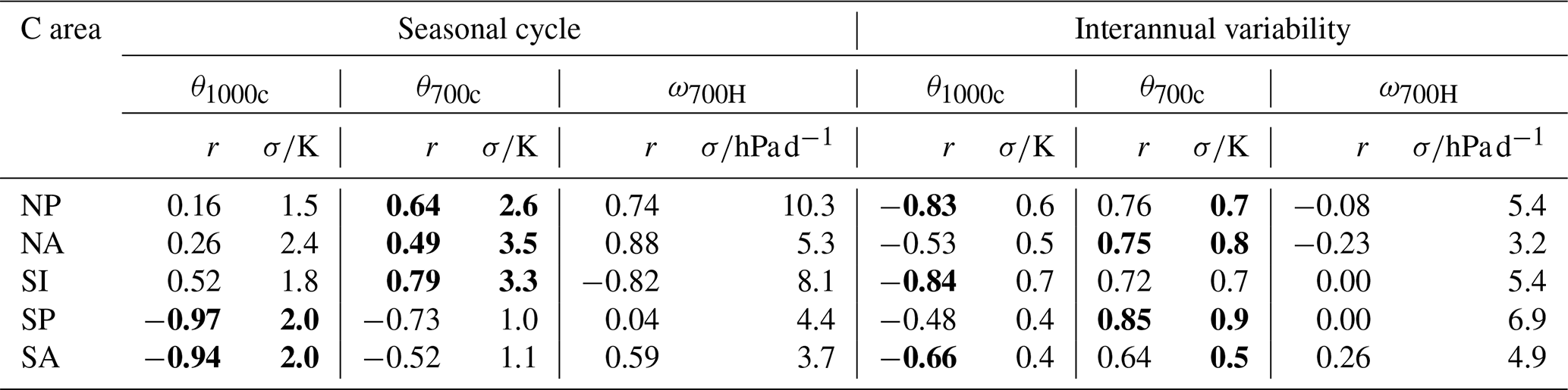
This analysis demonstrates that variations in EIS are complex and regionally dependent. It also hints at why previous studies have not reported a strong relationship between subtropical highs and cloudiness, as might be expected if, for instance, cloudiness was primarily controlled by either variations in temperatures at the surface, possibly driven by surface winds and ocean upwelling, or variations aloft, possibly driven by atmospheric subsidence. Using ω_700H as a factor of highs does not clearly indicate whether the variability of θ₇₀₀ is larger or smaller than that of θ₁₀₀₀. For the seasonal cycle, the three regions with the largest variability of the highs (measured by the standard variation in ω_700H in Table 1) are also the regions where θ₇₀₀ varies more than θ₁₀₀₀. However, this relationship does not necessarily indicate a causal link between subsidence rate in the highs and θ₇₀₀ because it does not hold on interannual timescales. Moreover, the correlation between ω_700H and EIS nearly vanishes, further suggesting that variations in atmospheric subsidence over H areas are not the cause of changes in EIS.

To explore whether such relationships might exist but are hidden by co-variability in other factors, we regress EIS against Q_c, the adiabatic warming in the cloud region, and two fields that could be indicative of the influence of the subtropical high on surface mechanisms, one being the LHF_c, which we expect to co-vary with the surface wind speed, $\Vert V\Vert$, and the other being ocean upwelling, w_E. Figure 3 shows that some weak relationships emerge, as expected. Greater adiabatic warming, stronger winds (as measured by surface latent heat fluxes), and more ocean upwelling are all positively correlated with increases in EIS. Because the relationships are generally stronger over the seasonal cycle as compared to the interannual record, it raises the question as to whether they are causal.

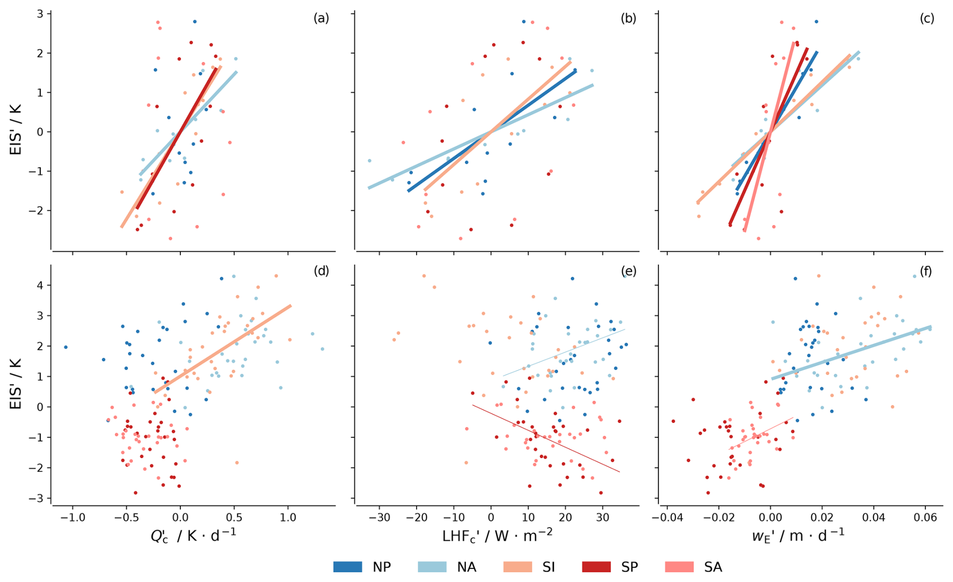
Figure 3 Scatter plots of Q and EIS (a, d), LHF and EIS (b, e), and w_E and EIS (c, f). The primes indicate deviations from the mean of the respective regions on the corresponding timescales. Each colour represents a region. The top branch is for the seasonal cycle, and the bottom branch is for the interannual time series. Regression lines are presented for p values ≤ 0.05 and are thicker when r²≥0.25.

3.2 Control by atmospheric subsidence

Before exploring to what extent variations in the high-pressure regions can explain variations in θ₇₀₀, we first examine the more basic question of whether the adiabatic warming, which in stationarity balances the diabatic cooling Q, co-varies with ω₇₀₀ in the Sc areas. Figure 4 demonstrates that there is a clear relationship between Q_c at 700 hPa and ω_700c in the climatological mean (Fig. 4). A strong and consistent relationship also emerges across the seasonal cycle and on interannual timescales (Fig. 5). Hence ω_700H is a good proxy for the adiabatic warming in the cloud areas.

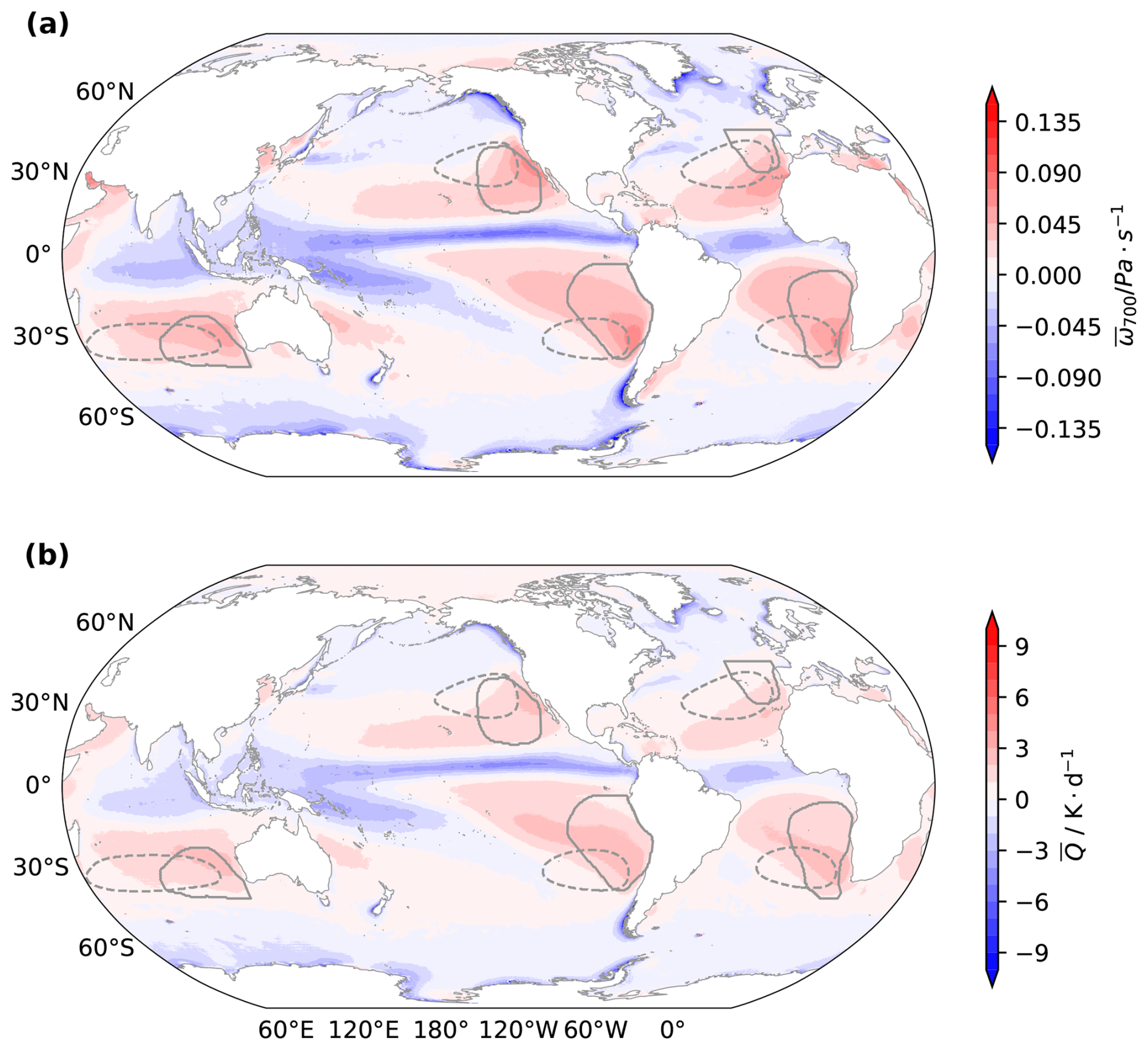
Figure 4 Map of 1985–2014 climatological mean ω₇₀₀ (a) and Q (b). Subtropical high areas are shown by dashed lines, and cloud regions are outlined by solid lines.

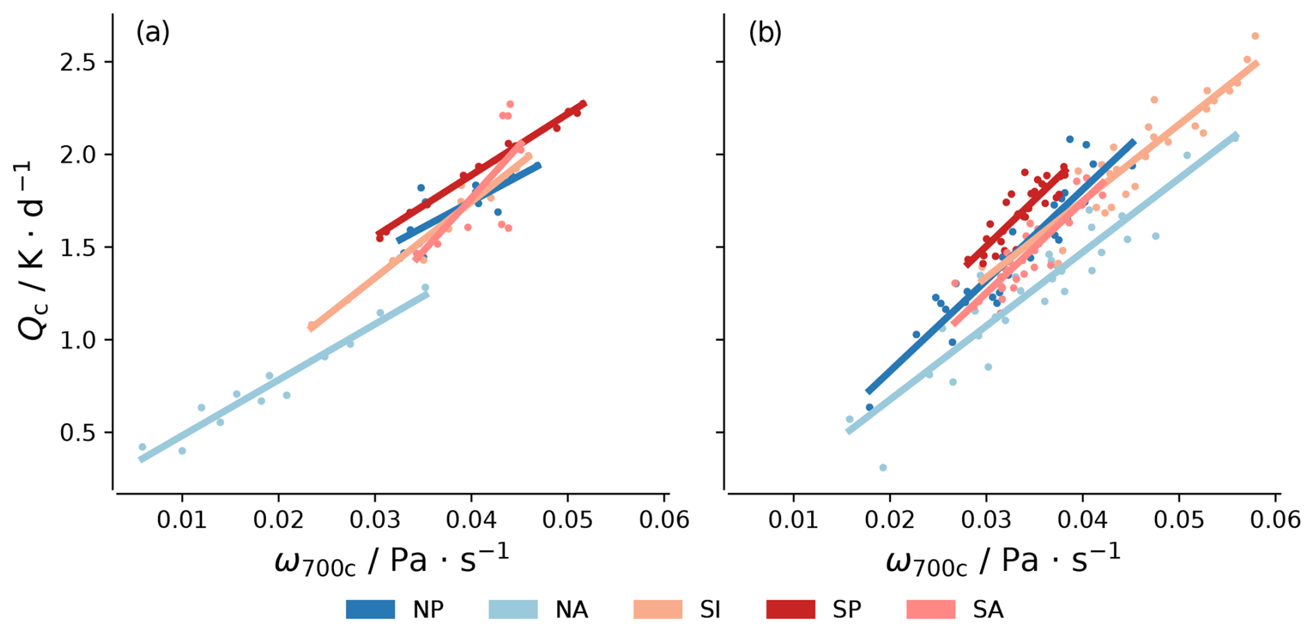
Figure 5 Scatter plots of ω₇₀₀ and Q. Subscript c denotes the mean value of the variable in the c area. Each colour represents a region. Panel (a) is for the seasonal cycle, and (b) is for the interannual time series. Regression lines are presented for p values ≤ 0.05 and are thicker when r²≥0.25.

Knowledge of adiabatic warming is, however, not sufficient to determine θ₇₀₀. This is shown in Fig. 6, which shows no consistent relationship between Q_c and θ_700c across the seasonal cycle for the different regions and no relationship between Q_c and θ_700c whatsoever on interannual timescales. This indicates that ω_700c is not the dominant factor for changes in θ₇₀₀ and falsifies the hypothesis that variations in θ_700c can be explained by a monsoon–desert mechanism, at least one mediated by adiabatic warming.

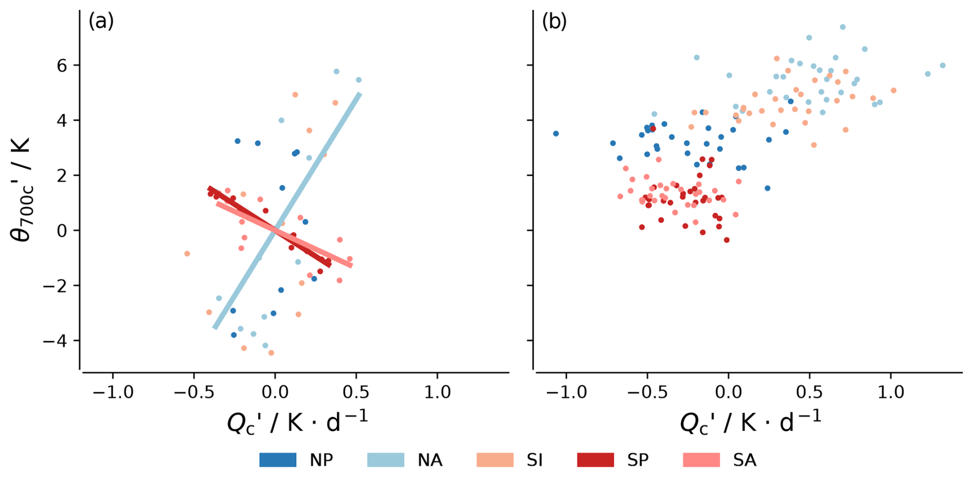
Figure 6 Scatter plots of Q and θ₇₀₀. The primes indicate deviations from the mean of the respective regions on the corresponding timescales. Subscript c denotes the mean value of the variable in the c area. Each colour represents a region. Panel (a) is for the seasonal cycle, and (b) is for the interannual time series. Regression lines are presented for p values ≤ 0.05 and are thicker when r²≥0.25.

3.3 Control by wind-driven cooling

In addition to subsidence rates, the steepness of subtropical highs is also proposed to influence EIS. As subtropical highs are typically located on the western flanks of Sc, the steepness of highs may affect the zonal geopotential gradient in c areas and thereby impact near-surface winds there. According to the Sverdrup balance, the equatorward near-surface wind, which in geostrophic balance is determined by the zonal geopotential gradient ($\frac{\mathrm{d}\mathrm{\Phi }}{\mathrm{d}x}$), is associated with a wind-stress gradient that results in ocean Ekman pumping (Anderson and Gill, 1975). In addition, the changed near-surface wind can also affect cold advection of waters from high latitudes and impact surface evaporative cooling as measured by the surface latent heat flux (LHF).

Figure 7 shows patterns for mean $\frac{\mathrm{d}\mathrm{\Phi }}{\mathrm{d}x}$, Ekman pumping velocity (w_E), and LHF. Unlike Q and ω₇₀₀, pattern correlations are difficult to discern. Ocean upwelling areas are restricted to the coastal regions where the wind-stress curl is large, and the maximum LHF is located on the west and equatorward side of the maximum $\frac{\mathrm{d}\mathrm{\Phi }}{\mathrm{d}x}$, where temperatures are warmer and strong trade winds prevail. A more quantitative evaluation of the relationship between $\frac{\mathrm{d}\mathrm{\Phi }}{\mathrm{d}x}$ and either w_E or LHF (not shown) does not show strong and consistent relationships across regions or timescales. This leads us to conclude that variations in near-surface geopotential gradients are not the primary driver of changes in θ₁₀₀₀ (Fig. 8) and hence variations in EIS.

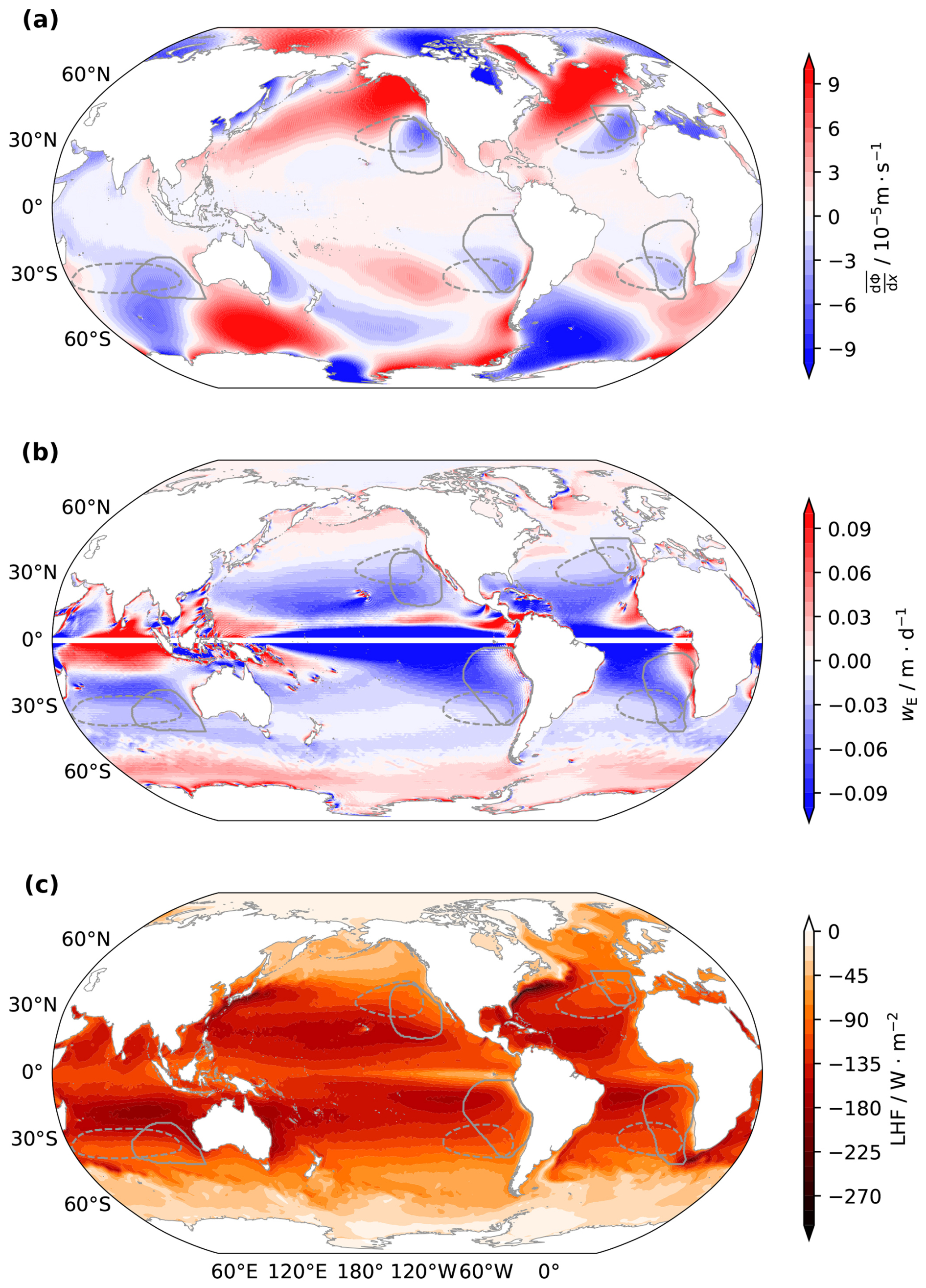
Figure 7 Map of 1985–2014 climatological mean (a) $\frac{\mathrm{d}\mathrm{\Phi }}{\mathrm{d}x}$, (b) w_E (masked within 1° N–1° S), and (c) LHF.

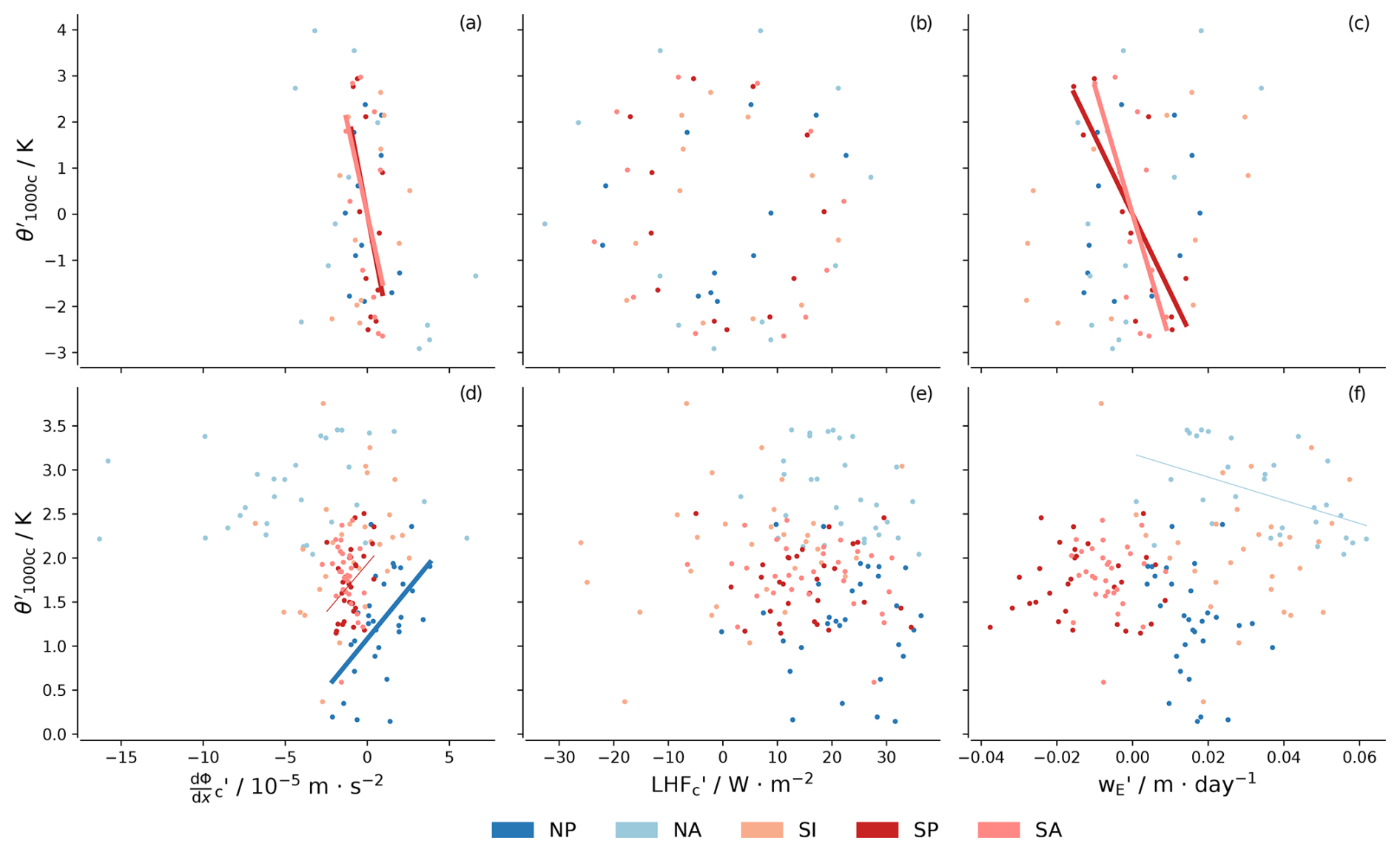
Figure 8 Scatter plots of $\frac{\mathrm{d}\mathrm{\Phi }}{\mathrm{d}x}$ and θ₁₀₀₀ (a, d), LHF and θ₁₀₀₀ (b, e), and w_E and θ₁₀₀₀ (c, f). Subscript c denotes the mean value of the variable in the c area, while w_E is averaged over the continuous ocean upwelling area near the coast. The primes indicate deviations from the mean of the respective regions on the corresponding timescales. Each colour represents a region. The top branch is for the seasonal cycle, and the bottom branch is for the interannual time series. Regression lines are presented for p values ≤ 0.05 and are thicker when r²≥0.25.

3.4 The disconnection between changes in H and c areas

Until this point we have considered proxies within c areas for the variation in H areas that generally lie westward of c areas. Figure 9 shows that subsidence in c areas is not necessarily a good proxy for subsidence in H areas and therefore not for the strength of the subtropical high represented by SLP_H, as no rule for the relationships between H and c areas emerges. Correlations, when they exist, can differ in sign across regions and for the same region across timescales. Even though the regression coefficients between the two areas show some similarity in NA across timescales, the correlations in the interannual time series are weak. Figure 10 also shows that the geopotential gradient in c areas does not consistently correlate with SLP in H areas. Therefore, the properties of c areas that may affect EIS do not simply follow the strength of subtropical highs, which further reduces the probability of predicting Sc by the variation in subtropical highs.

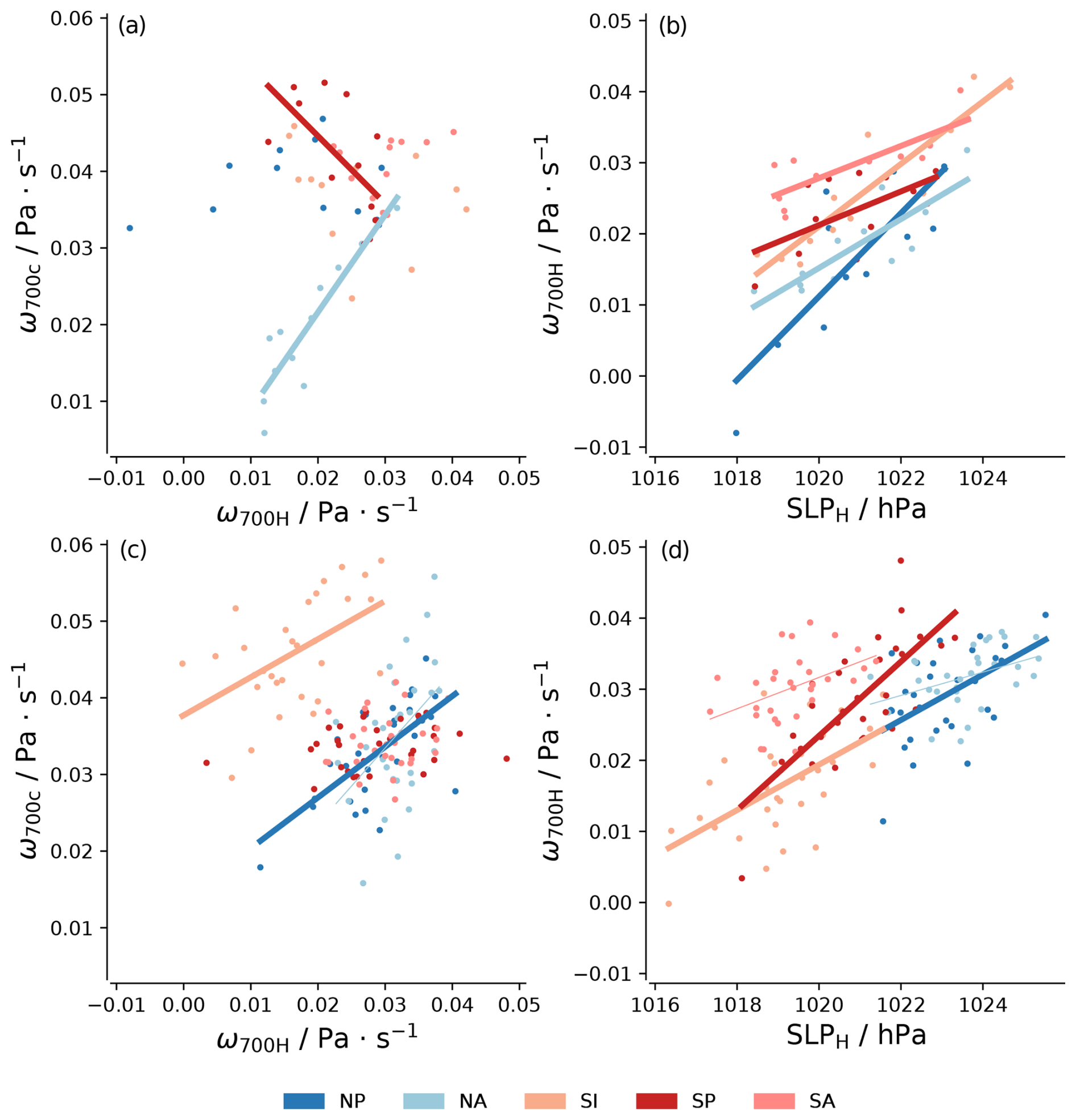
Figure 9 Scatter plots of ω₇₀₀ between H and c areas (a, c) and ω₇₀₀ and SLP in H areas (b, d). Each colour represents a region. The top branch is for the seasonal cycle, and the bottom branch is for the interannual time series. Regression lines are presented for p values ≤ 0.05 and are thicker when r²≥0.25.

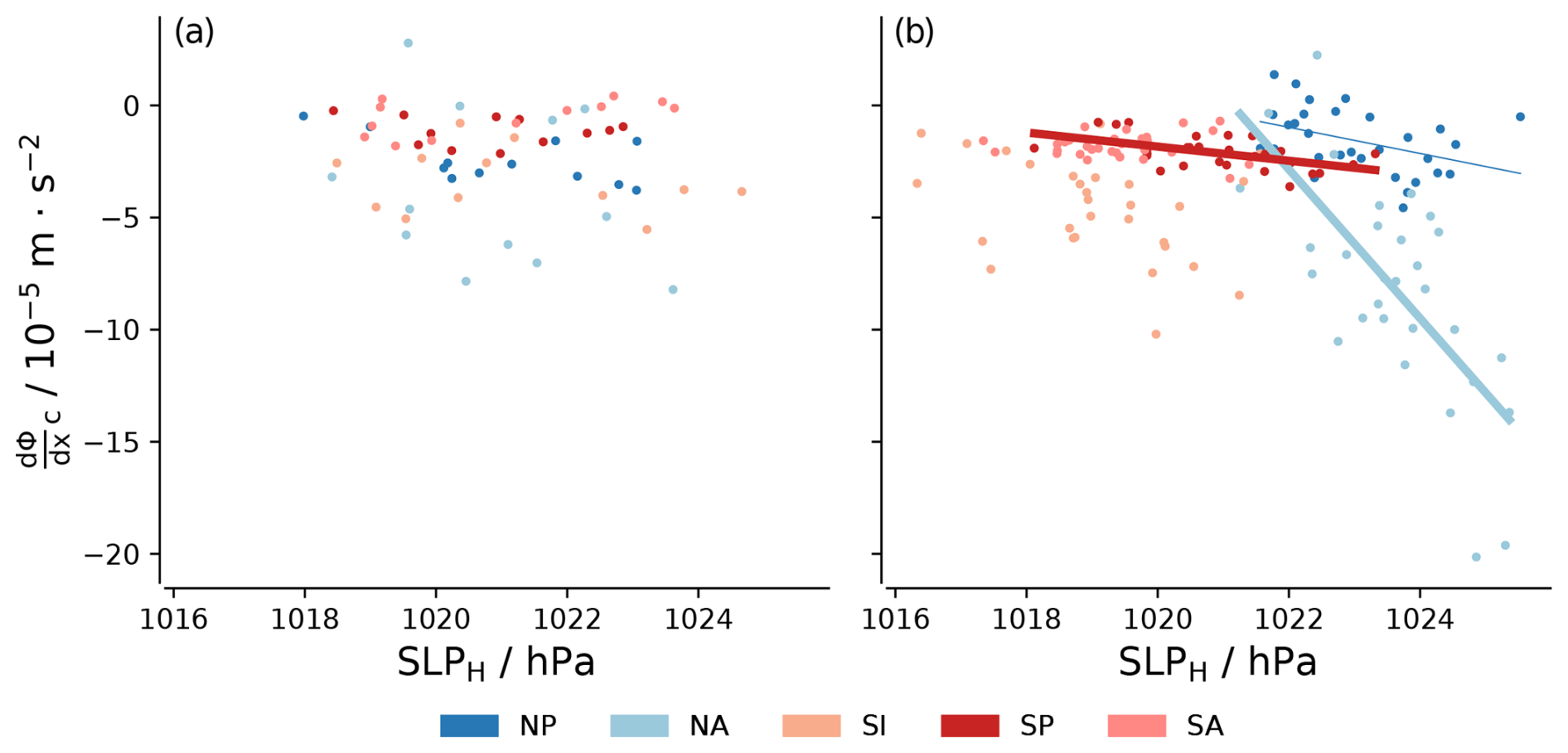
Figure 10 Scatter plots of $\frac{\mathrm{d}\mathrm{\Phi }}{\mathrm{d}x}$ in c areas and SLP in H areas on the seasonal (a) and interannual (b) timescales. Each colour represents a region. Regression lines are presented for p values ≤0.05 and are thicker when r²≥0.25.

4 Conclusions

This paper tests two hypothesized mechanisms by which subtropical highs may affect Sc. Both hypotheses are rejected. Figure 11 illustrates the relationships within the proposed mechanisms that are tested in this paper.

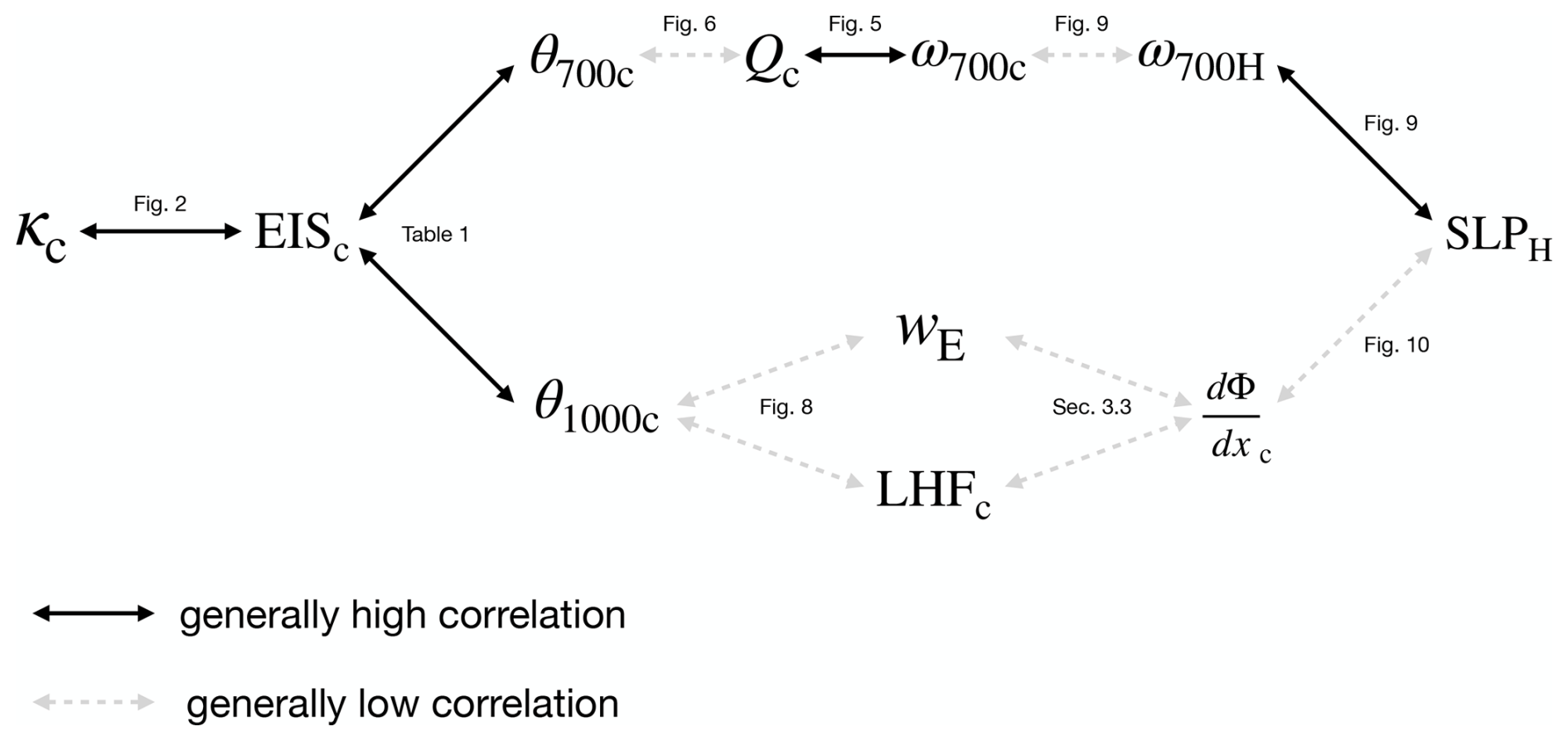
Figure 11 Schematic representation of temporal correlations analysed in this paper. Variables include κ (cloud fraction), EIS (estimated inversion strength), θ (potential temperature), Q (adiabatic warming), ω (subsidence rate), SLP (sea level pressure), w_E (Ekman pumping velocity in the associated coastal ocean upwelling areas), LHF (latent heat flux), and $\frac{\mathrm{d}\mathrm{\Phi }}{\mathrm{d}x}$ (700 hPa geopotential gradient). Subscript “H” represents the high-pressure areas, and “c” represents the Sc areas. Arrows indicate a general relationship; refer to the text for details.

First, we define the marine high-pressure areas and the Sc areas using a surface isobar in the case of the former and a satellite-derived cloud fraction in the latter. This identifies five regions, in each of which the high-pressure area intersects the Sc area, with the latter generally located on the eastward flanks of the former. Next, we demonstrate that Sc is well predicted by both the lower-tropospheric stability (LTS) and the estimated inversion strength (EIS). A more recent proposal for a cloud-controlling factor, the estimated cloud top entrainment index, is more complex as it includes humidity variations and does not perform better than the EIS, as its additional skill arises from predictions outside of the main cloud areas we consider. Furthermore, in the areas we consider, and for any particular region, most of the variability in EIS can be explained by LTS alone.

Given these findings, we hypothesize that EIS (or LTS) can be increased through an increase in adiabatic warming, Q, which maintains a higher potential temperature at 700 hPa. An enhanced subsidence in subtropical highs can lead to this increase in adiabatic warming. However, the variation in Q is not the dominant factor influencing changes in temperature above Sc (θ₇₀₀), as the correlation of θ₇₀₀ and adiabatic warming can even be negative in some regions. This agrees with Caldwell and Bretherton (2009), who show that the effects of the thermodynamic process do not warm the free troposphere directly; instead, they mostly enhance the subsidence itself, which – all things considered – would maintain a shallower cloud layer.

We further hypothesize that the steepness of the subtropical highs could modulate Sc amounts through their effect on the surface momentum balance, and hence surface temperature, to which θ₁₀₀₀ is strongly related. A high with a larger geopotential gradient in the Sc area is posited to increase surface wind speeds, enhancing ocean upwelling (w_E) along eastern coasts, accompanied by greater surface evaporation and cooling. If this mechanism were a dominant factor in controlling θ₁₀₀₀, we would expect strong relationships between θ₁₀₀₀ and both w_E and latent heat flux (LHF), as well as a correlation between geopotential gradient and w_E and even with LHF. However, there is little evidence supporting these relationships.

Environmental changes associated with variations in the subtropical high-pressure regions correlate better with LTS (and EIS) than with the components of the LTS and EIS the variations are thought to influence. On both seasonal and interannual timescales, regionally unified positive correlations between Q and EIS, as well as between ocean upwelling velocity and EIS, can be identified. We interpret this as indicative of variations in high-pressure regions not being the primary cause of variations in Q, w_E, and LHF but rather indicative of hidden mechanisms that cause these quantities to co-vary with LTS. This finding is further supported by the lack of robust relationships between the variations in Q, w_E, and LHF in the high-pressure region and the same quantity in the partially overlapping cloud regions.

Our results do not support the hypotheses that an understanding of how subtropical highs change with climate will be informative of how Sc amount will change in regions where such clouds prevail. It is well appreciated that the temperature control of the convecting areas on the moist adiabatic lapse rate throughout the tropics can influence the near-tropical LTS (Manabe et al., 1965; Stone and Carlson, 1979; Betts, 1986). However, there is also a growing appreciation of the departures from the weak temperature gradients that this mechanism relies on, which will continue to motivate efforts to identify dynamic factors influencing the LTS across the near tropics (Sobel and Bretherton, 2000; Sobel et al., 2001; Singh and O'Gorman, 2013; Bao and Stevens, 2021).