The biogeophysical effects of carbon fertilization of the terrestrial biosphere

The climate impacts of carbon fertilization of the terrestrial biosphere include cooling associated with the biogeochemical effects of enhanced land carbon storage, whereas the non-carbon-cycle biogeophysical effects associated with changes in surface energy and turbulent heat fluxes may warm or cool the climate system. Both of these effects may be dependent on the background climate. Here, I analyze state-of-the-art CMIP6 Earth system models that conducted simulations driven by 1 % yr⁻¹ increases in atmospheric carbon dioxide (CO₂) concentration that isolate the carbon fertilization effect (i.e., CO₂ radiative effects are not active) relative to a preindustrial background climate. At the time of CO₂ quadrupling, the biogeophysical effects yield multimodel global mean near-surface warming of 0.16±0.09 K, with 13 of the 15 models yielding warming. Using a Surface Energy Balance decomposition, most of this warming is associated with decreases in surface latent heat flux associated with reduced canopy transpiration. Decreases in surface albedo and increases in downwelling shortwave and longwave radiation – both of which are modulated by cloud reductions – are also associated with the warming. Overall, however, the biogeophysical warming is about an order of magnitude smaller than the corresponding cooling associated with enhanced land carbon storage at −1.38 K (−1.92 to −0.84 K). Simulations that isolate the carbon fertilization effect relative to a warmer, higher CO₂ background climate yield similar overall results. However, some nuances exist including stronger biogeophysical warming of the extratropics and weaker but nonsignificant biogeophysical warming of the tropics.

1 Introduction

Over land, increasing atmospheric CO₂ concentrations lead to carbon fertilization (e.g., Ainsworth and Long, 2005; Ainsworth and Rogers, 2007; Leakey et al., 2009; Norby and Zak, 2011). This effect involves physiological and structural vegetation changes including reduced stomatal conductance and increased photosynthesis rates, which are expected to increase net primary productivity (NPP) and carbon storage. However, the carbon fertilization effect depends on many factors, including plant species, temperature and availability of water and nutrients. The availability of soil inorganic nitrogen (N), for example, exerts a strong control on plant productivity and carbon storage in many temperate and boreal ecosystems (Vitousek and Howarth, 1991; Oren et al., 2001; Fernández-Martínez et al., 2014; Kicklighter et al., 2019). Climate change impacts (e.g., warming and altered precipitation patterns) on vegetation remain uncertain, but several studies suggest negative impacts on tropical biomass (e.g., Cox et al., 2004; Humphrey et al., 2018; Aleixo et al., 2019; del Rosario Uribe et al., 2023) including drought-induced tree mortality and loss of stored carbon (e.g., Lewis et al., 2011; Bonal et al., 2016; Corlett, 2016) but an increase in high-latitude biomass associated with warming and a longer growing season (Innes, 1991; Kauppi et al., 2014; D'Orangeville et al., 2016; Schaphoff et al., 2016). Nonetheless, intensification of terrestrial biospheric activity, including increased global photosynthesis and “greening” of the planet, has been found over the last few decades, with carbon fertilization likely playing a major role (Forkel et al., 2016; Thomas et al., 2016; Zhu et al., 2016; Campbell et al., 2017; Keeling et al., 2017; Haverd et al., 2020; Walker et al., 2021; Chen et al., 2022; Keenan et al., 2023).

Enhanced land carbon storage and greening of the terrestrial biosphere under elevated atmospheric CO₂ concentrations will promote a biogeochemically induced cooling effect. In other words, the carbon concentration feedback, which quantifies the carbon cycle's response to changes in atmospheric CO₂ concentration (expressed in units of carbon uptake/release per unit change in atmospheric CO₂ concentration) is negative from the atmosphere's perspective (Arora et al., 2020). Such changes in the terrestrial biosphere will also drive biogeophysical effects associated with surface energy and turbulent heat fluxes. For example, structural vegetation changes (e.g., enhanced leaf area index, LAI) associated with carbon fertilization will impact surface physical properties. This includes altered surface albedo (e.g., plants are darker than bare soil; Betts, 2000; Bala et al., 2006; Li et al., 2015), which promotes enhanced surface absorption of solar radiation and hence warming. Furthermore, the physiological changes of carbon fertilization (i.e., reduced stomatal conductance and enhanced water use efficiency) are associated with reduced plant transpiration and latent heat flux, which directly impact surface temperature (i.e., less evapotranspiration implies surface warming) as well as atmospheric water vapor and clouds (Field et al., 1995; Bounoua et al., 1999; Boucher et al., 2009; Cao et al., 2009; Cao et al., 2010; Doutriaux-Boucher et al., 2009; Skinner et al., 2018; Zarakas et al., 2020). Plant physiological responses to CO₂ also have large impacts on the continental hydrologic cycle, with a dominant role in reducing not only evapotranspiration but also runoff (Lemordant et al., 2018) and reducing predictions of future drought stress (Swann et al., 2016).

It is well established that vegetation physiological changes under enhanced atmospheric CO₂ concentrations lead to surface warming. Sellers et al. (1996) used the coupled biosphere–atmosphere model (SiB2-GCM) to show that under doubled atmospheric CO₂ concentrations, physiological changes in vegetation led to surface warming (by about 0.1 K globally), consistent with decreases in evapotranspiration. This result is supported by several subsequent studies (e.g., Boucher et al., 2009; Cao et al., 2010; Arora et al., 2013; Arora et al., 2020; Zarakas et al., 2020). For example, Cao et al. (2010) used the Community Land and Community Atmosphere Model to show, under a doubling of atmospheric CO₂, that the physiological effects of CO₂ lead to surface warming of 0.42±0.02 K. Using the HadCM3LC version of the Met Office Unified Model System, Doutriaux-Boucher et al. (2009) showed that this physiologically induced warming effect is also related to a reduction in low cloud cover (and, in turn, enhanced surface shortwave radiation). The more recent, multimodel study of Zarakas et al. (2020) found model mean warming of 0.14 K (standard deviation of 0.16 K) in CMIP6 models and 0.14 K (standard deviation of 0.11 K) in CMIP5 models (again, centered on the time of CO₂ doubling). Thus, although analyses on this topic have been performed, there is a lack of a systematic analysis of the mechanisms by which carbon fertilization impacts the climate system, particularly from a multimodel perspective. Moreover, prior studies have not attempted to investigate how robust the climate effects of carbon fertilization are to the background climate state.

In this paper, I use Coupled Model Intercomparison Project phase 6 (CMIP6; Eyring et al., 2016) models to quantify the climate effects of carbon fertilization (i.e., in the absence of the direct radiative effects of CO₂). Novelties of this study include the use of the Surface Energy Balance (SEB) decomposition (Luyssaert et al., 2014; Hirsch et al., 2018; Boysen et al., 2020) to infer the contribution of changes in energy fluxes to changes in surface temperature, which enables more detailed insights into the mechanisms by which CO₂ fertilization impacts the climate system – this includes the importance of surface turbulent heat fluxes and surface radiative fluxes, as well as clouds. Furthermore, to understand if the climate effects of carbon fertilization are robust to the background climate, the analysis is performed under both a preindustrial background climate and a warmer (higher atmospheric CO₂ concentration) background climate. Additional novelties of this study include the investigation of the vegetation–aerosol response to carbon fertilization under increasing CO₂ and analysis of the intermodel variation in the vegetation and climate responses (e.g., comparing models with and without a terrestrial nitrogen cycle).

Climate effects include the directly simulated biogeophysical (non-carbon-cycle) temperature response, while I infer the biogeochemical temperature response. Consistent with the above studies (e.g., Boucher et al., 2009; Cao et al., 2009, 2010; Doutriaux-Boucher et al., 2009; Zarakas et al., 2020), I find significant global mean biogeophysical warming, largely driven by reductions in latent heat flux associated with decreases in canopy transpiration. Decreases in surface albedo and increases in downwelling shortwave and longwave radiation, both of which are modulated by cloud reductions, are also associated with the warming. The magnitude of this biogeophysical warming, however, is about an order of magnitude smaller than the inferred biogeochemical cooling associated with enhanced land carbon storage. Similar results are obtained under both the preindustrial and warmer background climate but with some nuances.

2 Methods

2.1 CMIP6 models and 1 % yr⁻¹ simulations

CMIP6 (Eyring et al., 2016) performed three sets of 1 % yr⁻¹ increasing atmospheric CO₂ concentration simulations, which are initialized from the preindustrial CO₂ concentration of ∼ 284 ppm and integrated for 150 years. The default 1 % yr⁻¹ simulations (abbreviated as FULL) are fully coupled as the radiation and carbon cycle components see the increasing CO₂ concentration. Two variants of the 1 % yr⁻¹ simulation were performed as part of the Coupled Climate–Carbon Cycle Model Intercomparison Project (C4MIP; Jones et al., 2016), including a biogeochemically coupled version (abbreviated here as PHYS) and a radiatively coupled version (abbreviated here as RAD). Under PHYS, only the carbon cycle components (both land and ocean) respond to the increase in CO₂, while the atmospheric radiative transfer calculations use a CO₂ concentration that remains at the preindustrial concentration. Under RAD only the atmospheric radiation code sees the increase in CO₂, and the carbon cycle components see the fixed, preindustrial CO₂ concentration.

The primary focus of this analysis is the PHYS runs, which allows assessment of the climate responses associated with the carbon cycle under elevated CO₂ (without the influence of CO₂ radiative effects) relative to a preindustrial (PI) background climate. Over land, this effect is traditionally referred to as carbon fertilization of the terrestrial biosphere (e.g., Ainsworth and Long, 2005; Ainsworth and Rogers, 2007; Forkel et al., 2016; Thomas et al., 2016; Zhu et al., 2016, Campbell et al., 2017; Chen et al., 2022). In particular, this includes changes in vegetation physiology including photosynthesis, transpiration and stomatal conductance, and changes in vegetation state (e.g., leaf area index, canopy height). In models with dynamic vegetation, this also includes changes in vegetation type and coverage. These changes in turn affect surface radiative and turbulent heat fluxes, which impact surface temperature and other aspects of climate. As the three sets of 1 % yr⁻¹ simulations are CO₂ concentration driven (as opposed to emissions driven), the simulated climate responses include only the biogeophysical effects (e.g., changes in surface fluxes and more generally all non-carbon-cycle effects). The climate impacts associated with changes in terrestrial carbon pools (biogeochemical effects) are not allowed to feedback onto the climate system (i.e., enhanced land carbon storage under elevated CO₂ does not impact the atmospheric CO₂ concentration and thus does not impact climate). However, as discussed below, the surface temperature responses to changes in terrestrial carbon pools can be inferred from the transient climate response to cumulative CO₂ emissions (TCRE; Gillett et al., 2013; Arora et al., 2020; Boysen et al., 2020).

This analysis uses up to 15 CMIP6 models (Table S1). Responses are estimated from years 101–140 (CO₂ quadruples in year 140) in the PHYS runs relative to the corresponding 40 years in the preindustrial control simulation (PHYS-PI). I refer to this 40-year time period as the time of CO₂ quadrupling. Preindustrial control simulations feature fixed (to the preindustrial value) atmospheric CO₂ concentration and other climate drivers (e.g., other greenhouse gases, solar irradiance, aerosols). Monthly mean data are used, and all data are interpolated to a 2.5° × 2.5° grid and aggregated to annual means. Only two models, GFDL-ESM4 and MPI-ESM1-2-LR, include dynamic vegetation (i.e., vegetation type and coverage can respond to the elevated CO₂). Three models, GFDL-ESM4, UKESM1-0-LL and NorESM2-LM, include atmospheric chemistry with an interactive representation of vegetation biogenic volatile organic compound (BVOC) feedbacks (e.g., Gomez et al., 2023). Eight models (ACCESS-ESM1-5, CESM2, CMCC-ESM2, EC-Earth3-CC, MIROC-ES2L, MPI-ESM1-2-LR, NorESM2-LM and UKESM1-0-LL) feature a terrestrial nitrogen cycle (Table S1). Additional model information can be found in Arora et al. (2020), Gomez et al. (2023), Allen et al. (2024) and Gier et al. (2024).

In addition, I quantify the biogeophysical and biogeochemical effects of carbon fertilization under a warmer (higher atmospheric CO₂ concentration) background climate. This analysis is analogous to that above, except here the signal is estimated as the difference between the fully coupled and radiatively coupled 1 % yr⁻¹ increasing atmospheric CO₂ concentration simulations (i.e., FULL-RAD). Thirteen models are available for this analysis (MRI-ESM2-0 and EC-Earth3-CC are missing). The double difference, i.e., (FULL-RAD) − (PHYS-PI), represents the influence of the carbon fertilization effect within the context of a warmer climate. All analyses that quantify the influence of the carbon fertilization effect within the context of a warmer climate, i.e., (FULL-RAD) − (PHYS-PI), are based on the same 13 models available for all four simulations. I note that carbon cycle feedbacks possess nonlinearity; i.e., the sum of RAD and PHYS has been shown to differ from FULL. For example, Zickfeld et al. (2011) showed that the carbon sinks on land and ocean are less efficient when exposed to the combined effect of elevated CO₂ and climate change (FULL) than to the sum of the two (RAD+PHYS), with land accounting for the bulk of this nonlinearity due to the presence or absence of the carbon fertilization effect.

2.2 Surface Energy Balance decomposition

The Surface Energy Balance (SEB) decomposition (Luyssaert et al., 2014; Hirsch et al., 2018; Boysen et al., 2020) is used to infer the contribution of changes in energy fluxes to changes in surface temperature (ΔTS):

$$\begin{array}{}\text{(1)}& \begin{array}{rl}\mathrm{\Delta }\mathrm{TS}=& {\displaystyle \frac{\mathrm{1}}{\mathrm{4}\mathit{ϵ}\mathit{\sigma }{\mathrm{TS}}_{\mathrm{control}}^{\mathrm{3}}}}\left[\mathrm{\Delta }\mathrm{SWD}\left(\mathrm{1}-\mathit{\alpha }\right)-\mathrm{\Delta }\mathit{\alpha }\left(\mathrm{SWD}\right)\right.\\ & \left.+\mathrm{\Delta }\mathrm{LWD}-\mathrm{\Delta }\mathrm{LH}-\mathrm{\Delta }\mathrm{SH}\right],\end{array}\end{array}$$

where ε is the surface emissivity assumed to be 0.97 (Boysen et al., 2020), σ is the Stefan–Boltzmann constant with a value of $\mathrm{5.67}\times {\mathrm{10}}^{-\mathrm{8}}$ W m⁻² K⁻⁴ and TS_control is the surface temperature from the preindustrial control experiment. The first term in square brackets, which is denoted throughout the paper as SWD_SEB, represents the contribution from changes in downwelling surface shortwave radiation (ΔSWD), which is multiplied by the monthly mean climatology of (− α); the second term is denoted as α_SEB and represents the contribution from changes in surface albedo (α), which is multiplied by the monthly mean SWD climatology (changes in albedo impact upwelling surface shortwave radiation); the third term is denoted as LWD_SEB and represents the contribution from changes in downwelling surface longwave radiation (ΔLWD); the fourth term is denoted as LHF_SEB and represents the contribution from changes in surface latent heat flux (ΔLHF); and the final term, which is denoted throughout the paper as SHF_SEB, represents the contribution from changes in surface sensible heat flux (ΔSHF). I also decompose the first term on the right (i.e., SWD_SEB) into the contribution from changes in surface downwelling shortwave radiation under clear-sky (SWDCLR_SEB) and cloudy-sky (SWDCLD_SEB) conditions. The clear-sky contribution is estimated as ΔSWDCLR(1−α), where ΔSWDCLR is the change in clear-sky downwelling surface solar radiation. The cloudy-sky contribution is estimated as the residual between SWD_SEB and SWDCLR_SEB. A similar decomposition is performed for downwelling surface longwave radiation to isolate its clear-sky (LWDCLR_SEB) and cloudy-sky contributions(LWDCLD_SEB). Furthermore, LHF_SEB is decomposed into contributions from transpiration (TRAN_SEB) and evaporation + sublimation (EVAP_SEB). The SEB decomposition is performed over all land areas. I note that the SEB decomposition does not account for all factors, including for example the ground heat flux and changes in subsurface heat storage (both of which are assumed to be zero here) or changes in surface emissivity.

2.3 Statistical significance

Statistical significance of a response is estimated using two approaches. In the first approach (e.g., Fig. 1), the multimodel mean time series for the experiment and the control is calculated, and their difference is computed. A two-tailed pooled t test is used to assess significance of this difference at the 90 % confidence level with $n_{\mathrm{1}}+n_{\mathrm{2}}-\mathrm{2}$ degrees of freedom (n₁ is the number of years in the experiment and n₂ is the number of years in the control, i.e., 40 years each) using the pooled variance $\frac{(n_{\mathrm{1}}-\mathrm{1})S_{\mathrm{1}}^{\mathrm{2}}+(n_{\mathrm{2}}-\mathrm{1})S_{\mathrm{2}}^{\mathrm{2}}}{n_{\mathrm{1}}+n_{\mathrm{2}}-\mathrm{2}}$, where S₁ and S₂ are the sample variances. Significance of the multimodel mean response relative to each individual model response (e.g., Table S2) is estimated by comparing the average of the individual model responses relative to its uncertainty, estimated as ±1.65 × SE (i.e., the 90 % confidence interval). SE is the standard error estimated as $\frac{\mathrm{1.65}\times \mathit{\sigma }}{\sqrt{m}}$, where σ is the standard deviation across models and m is the number of models. Model agreement on the sign of the multimodel mean response is spatially and globally estimated as the percentage of models that yield a positive or negative response. A two-tailed binomial test yields model agreement at the 90 % confidence level when at least 11 of the 15 (73 %) models agree on the sign of the response.

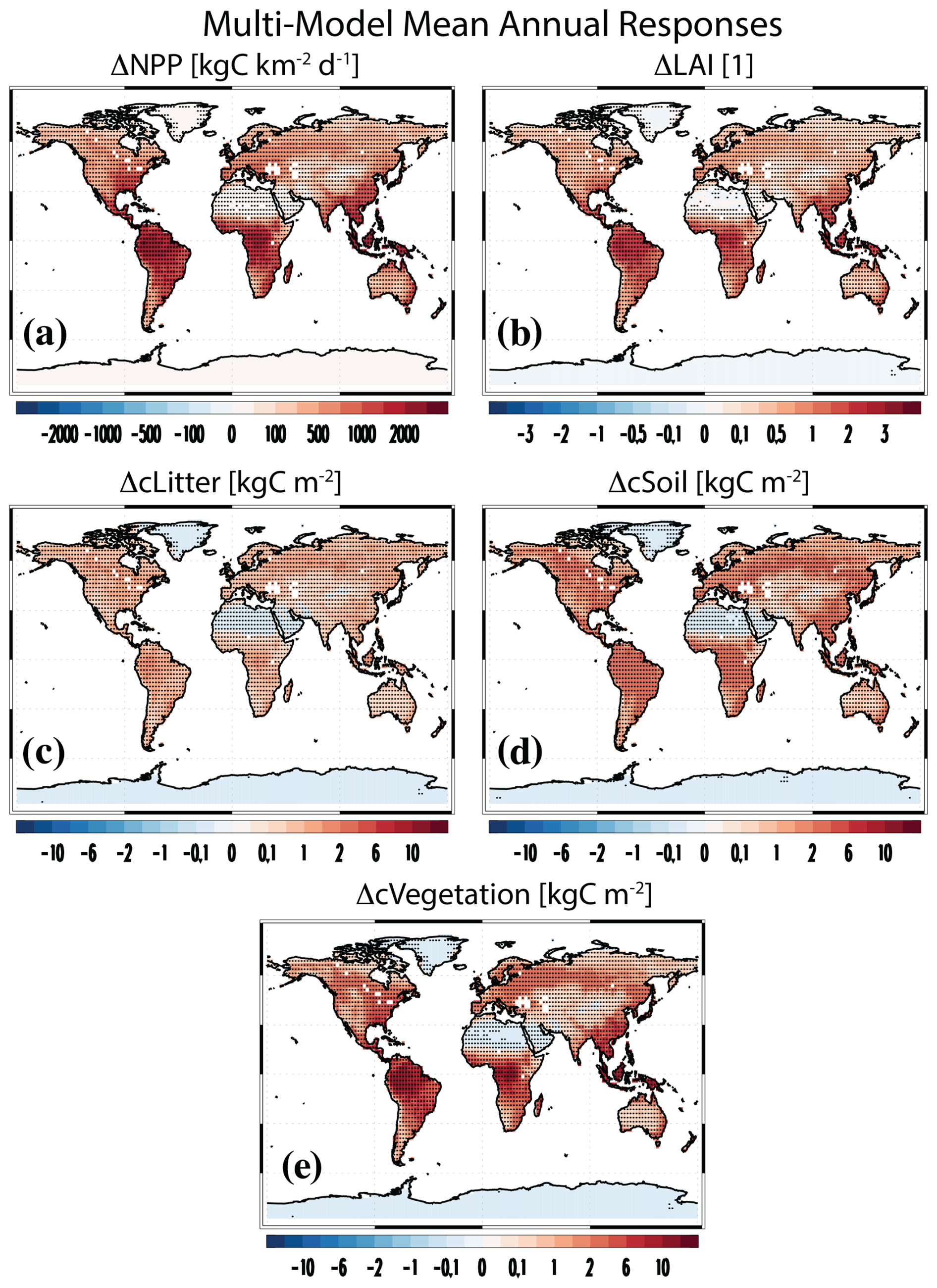
Figure 1 Vegetation and land carbon responses. Multimodel mean annual mean PHYS-PI responses for (a) net primary productivity (NPP; kg C km⁻² d⁻¹), (b) leaf area index (LAI; dimensionless), (c) litter pool carbon (cLitter; kg C m⁻²), (d) soil pool carbon (cSoil; kg C m⁻²) and (e) vegetation carbon (cVegetation; kg C m⁻²). Symbols denote a response significant at the 90 % confidence level based on a two-tailed pooled t test.

There are two types of correlations (r) used throughout this paper. One is a spatial correlation between multimodel mean responses. Here, the multimodel mean responses at each grid box are first calculated, and then a regional (e.g., global/tropical/extratropical) correlation is estimated. The second type is the intermodel correlation between model mean responses. Here, each model's grid box or regional (e.g., tropical) response is first estimated, and then a correlation across models for that grid box (or region) is calculated. Significance of correlations is estimated from a two-tailed t test as $t=\frac{r}{\sqrt{\frac{\mathrm{1}-r^{\mathrm{2}}}{N-\mathrm{2}}}}$, with N−2 degrees of freedom. N is either the number of grid boxes (for a spatial correlation) or the number of models (for correlations across models).

3 Results

3.1 Vegetation, land carbon and inferred biogeochemical temperature responses

Figure 1 shows multimodel mean annual mean responses of vegetation including NPP and LAI. The global mean increase in NPP is 679.4±140.6 kg km⁻² d⁻¹ (77.4 % increase relative to the control), with larger increases in the tropics (30° S–30° N) at 1049.7±248.2 kg km⁻² d⁻¹ as compared to the extratropics (30–60° S and 30–60° N) at 516.7±109.4 kg km⁻² d⁻¹ (Table S2). In each of these regions, all 15 models agree on a positive NPP response (Fig. S1 shows the spatial model agreement on the sign of the response). Similar results exist for LAI, with a multimodel mean global mean increase of 0.71±0.25 (Fig. 1b; 48.9 % increase relative to the control), which increases to 1.12±0.41 in the tropics. Here, however, one model features a (very small) decrease in LAI; i.e., the GISS-E2-1-G LAI response is essentially zero at −0.00065. GISS-E2-1-G prescribes fixed monthly LAI, so this model does not capture the impact of carbon fertilization on LAI (Ito et al., 2020). One of the two models with interactive vegetation, GFDL-ESM4, yields relatively large global mean NPP increases (second largest) at 1207.3±30.9 kg km⁻² d⁻¹ (global mean), whereas MPI-ESM1-2-LR yields 673.2±13.9 kg km⁻² d⁻¹, a value close to the multimodel global mean increase. In terms of LAI, GFDL-ESM4 yields a value close to the multimodel global mean at 0.84±0.02, while MPI-ESM1-2-LR yields the weakest global mean increase at 0.17±0.01.

In terms of land carbon (cLand), the multimodel annual mean global mean increase is 4.52±0.68 kg C km⁻², and all 14 models (GISS-E2-1-G is missing) agree on enhanced land carbon sequestration. Decomposing land carbon into vegetation, soil organic matter and litter carbon shows that the bulk of this increase is due to an increase in vegetation carbon (Fig. 1e) at 2.48±0.42 kg C km⁻² (75.1 % increase relative to the control). This is followed by an increase in soil organic matter carbon (Fig. 1d) at 1.38±0.49 kg C km⁻² (15.0 % increase relative to the control) and litter carbon (Fig. 1c) at 0.66±0.22 kg C km⁻² (64.4 % increase relative to the control). Converting the above land carbon responses into multimodel mean global totals yields 468.1±89.4, 248.0±89.5 and 119.1±45.2 Pg C for vegetation carbon, soil carbon and litter carbon, respectively. Thus, the total land carbon increase is 835.3±134.3 Pg C. Increases in vegetation carbon contribute 56 % to this value, followed by soil carbon at 30 % and litter carbon at 14 %. Once again, models with interactive vegetation do not stand out, as GFDL-ESM4 yields a total land carbon increase of 958.6±32.6 Pg C, and MPI-ESM1-2-LR yields 530.7±12.0 Pg C (fourth smallest increase).

I separate the models into the eight (N models) that have a representation of the terrestrial nitrogen cycle versus the six models (noN models) that do not (GISS-E2-1-G is missing so there are only 14 models). As noted in Gier et al. (2024), the inclusion of nitrogen limitation led to a large improvement in photosynthesis compared to models not including this process.

I find significantly larger increases in land carbon storage in noN models at 1153.4±213.6 Pg C versus 581.6±157.5 Pg C in N models (consistent with Arora et al., 2020). Similar statements apply for NPP (923.4±202.2 kg km⁻² d⁻¹ in noN models versus 679.4±140.6 kg km⁻² d⁻¹ in N models) and LAI (0.94±0.48 in noN models versus 0.62±0.24 in N models). The weaker increase in land carbon storage in models with a terrestrial nitrogen cycle is consistent with terrestrial nitrogen generally reducing the response of NPP and carbon storage to elevated levels of atmospheric CO₂ because of an increasing limit of nitrogen availability for carboxylation enzymes and new tissue construction (e.g., Jones et al., 2016).

I use the TCRE (Gillett et al., 2013; Arora et al., 2020; Boysen et al., 2020) to estimate the near-surface air temperature (TAS) response to the aforementioned changes in land carbon (biogeochemical effects). The TCRE quantifies the amount of warming relative to the preindustrial state per unit cumulative emissions at the time when atmospheric CO₂ concentration doubles in FULL. The best estimate of the TCRE at 1.65 K per 1000 Pg C, with a likely range from 1.0 to 2.3 K per 1000 Pg C (Canadell et al., 2021), yields a biogeochemical cooling effect of −1.38 (−1.92 to −0.84) K. Models without a terrestrial nitrogen cycle (consistent with their enhanced land carbon storage) yield larger cooling (but not significantly so) at −1.90 (−2.65 to −1.15) K relative to the models with a terrestrial nitrogen cycle at −0.96 (−1.34 to −0.58) K. Similar biogeochemical cooling is obtained if I use an estimate of each model's TCRE (as opposed to the best estimate) at −1.22 K for all models, −1.70 K for noN models and −0.86 K for N models. Thus, the cooling difference between models with and without a terrestrial nitrogen cycle is largely due to differences in the land carbon response.

Thus, carbon fertilization at the time of CO₂ quadrupling yields large increases in land carbon storage and corresponding global mean biogeochemical cooling as inferred from the TCRE. Models that lack a terrestrial nitrogen cycle tend to yield larger increases in land carbon storage and, in turn, larger inferred cooling, implying they may overestimate the magnitude of this cooling effect. I note that the magnitude of this multimodel biogeochemical mean cooling is relatively large; e.g., it is about 35 % of the global mean warming under FULL of 3.94±0.37 K.

3.2 Biogeophysical temperature responses

Figure 2a shows the multimodel annual mean near-surface air temperature response. As noted above, the simulated temperature responses in these simulations only include the biogeophysical (non-carbon-cycle) effects. The multimodel annual mean global mean TAS response is 0.16±0.09 K, with 13 of the 15 models yielding warming (Fig. 2b shows the spatial model agreement on the sign of the response). The largest warming occurs in EC-Earth3-CC at 0.51±0.05 K, followed by CESM2 at 0.44±0.04 K and UKESM1-0-LL at 0.40±0.04 K (Fig. S2). The two models that yield cooling are CMCC-ESM2 and CNRM-ESM2-1 at $-\mathrm{0.01}\pm \mathrm{0.07}$ (not significant at the 90 % confidence level) and $-\mathrm{0.31}\pm \mathrm{0.04}$ K, respectively (Fig. S2e, f). Over land, the multimodel mean warming increases to 0.28±0.13 K (14 of the 15 models yield warming). In both cases, warming is larger in the extratropics as compared to the tropics (Table S3). Thus, biogeophysical effects of carbon fertilization yield warming but much less as compared to the corresponding biogeochemical effects noted above at −1.38 (−1.92 to −0.84) K. I also note that the biogeophysical warming of carbon fertilization is much smaller as compared to the biogeophysical warming associated with the radiative effects (from RAD-PI) of CO₂ at 3.78±0.35 K.

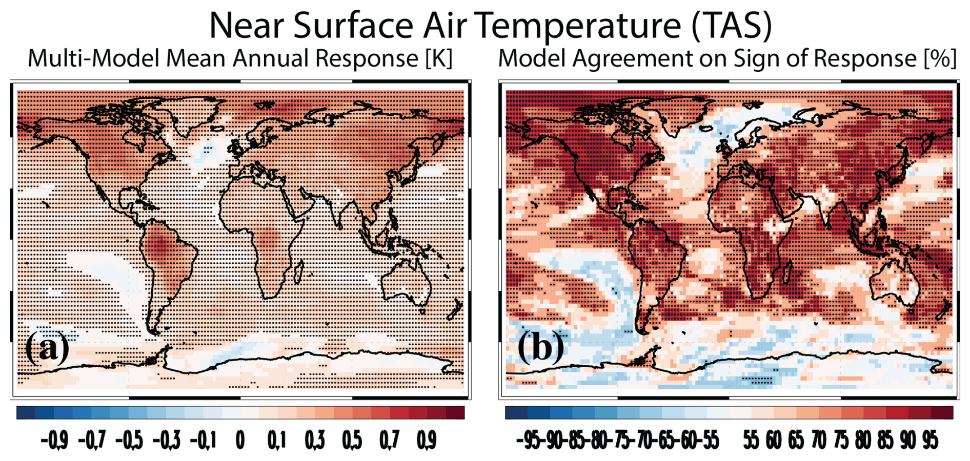
Figure 2 Near-surface air temperature. (a) Multimodel mean annual mean near-surface air temperature (TAS; K) PHYS-PI response. Symbols denote a response significant at the 90 % confidence level based on a two-tailed pooled t test. (b) Model agreement on the sign of the TAS response [% of models]. Red (blue) colors indicate model agreement on an increase (decrease). Symbols represent significant model agreement at the 90 % confidence level based on a two-tailed binomial test.

3.3 Drivers of the biogeophysical temperature response

I use the Surface Energy Balance (SEB; Sect. 2.2) decomposition (Luyssaert et al., 2014; Hirsch et al., 2018; Boysen et al., 2020) to understand the drivers of the biogeophysical temperature changes. I first note that the SEB decomposition reasonably reproduces the change in surface temperature (TS) and TAS. For example, the SEB-reconstructed multimodel annual mean global land mean TS response is 0.33±0.13 K relative to the actual TS and TAS responses of 0.26±0.12 and 0.28±0.13 K, respectively (Table S4).

Figure 3 shows multimodel annual mean spatial responses for the main terms of the SEB decomposition (Fig. S3 shows the corresponding model agreement on the sign of the responses, and Fig. S4 shows a bar chart of the SEB responses). LHF_SEB (Fig. 3d) contributes the most to the global land surface warming at 0.27±0.11 K (Table S4), followed by LWD_SEB (Fig. 3c) at 0.20±0.13 K. α_SEB (Fig. 3a) contributes 0.11±0.06 K, and SWD_SEB (Fig. 3b) contributes 0.09±0.06 K. In contrast, SHF_SEB (Fig. 3e) leads to cooling at $-\mathrm{0.34}\pm \mathrm{0.08}$ K. Model agreement on the sign of the multimodel mean response occurs in 12 to 13 of the 15 models (depending on the SEB term; Table S4). As with the global land mean, LHF_SEB contributes the most to the tropical land mean warming at 0.45±0.15 K (14/15 models agree on warming). Over extratropical land, the dominant SEB terms are LWD_SEB (0.20±0.16 K), as well as α_SEB (0.16±0.09 K) and SW_SEB (0.16±0.10 K).

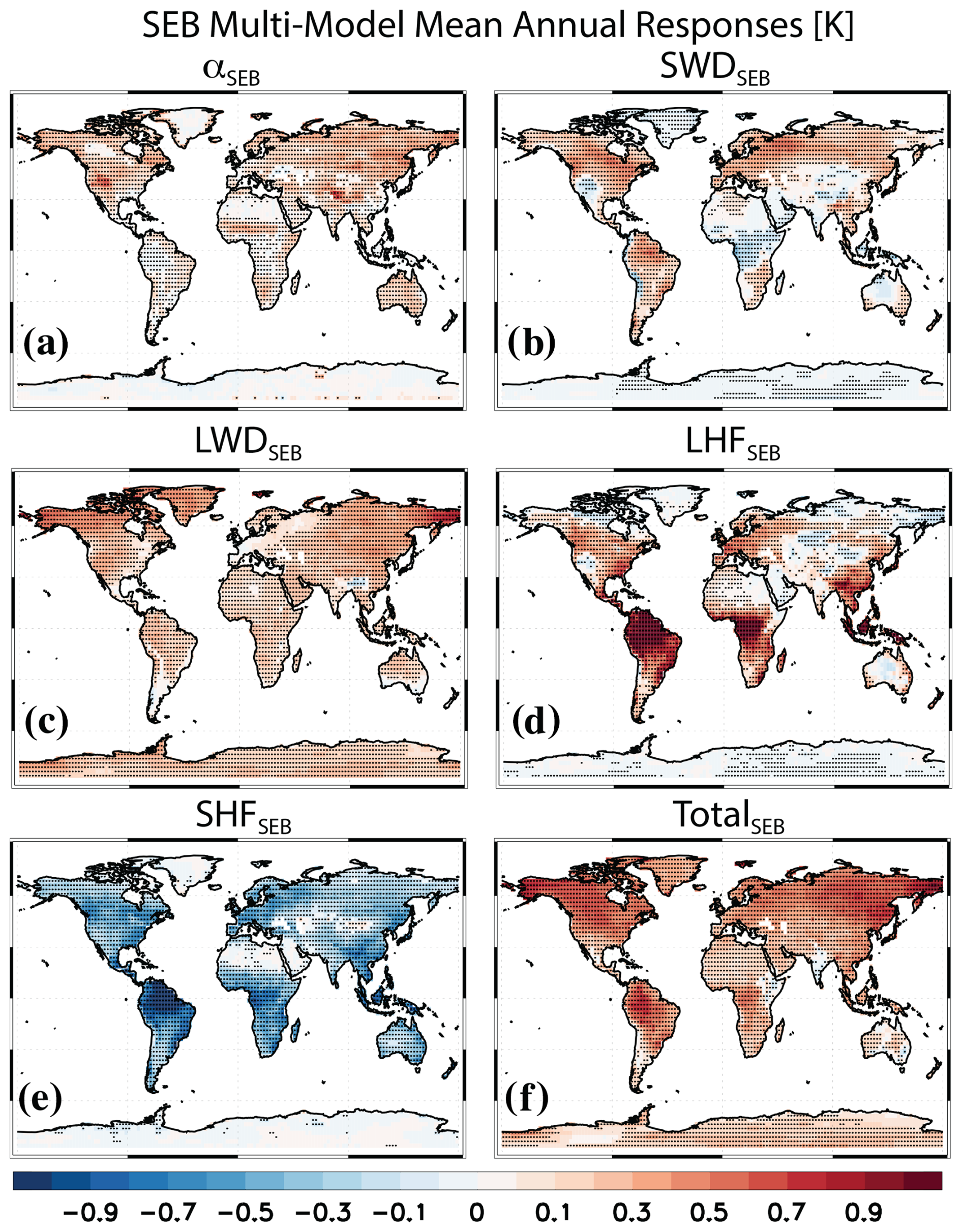
Figure 3 Surface energy balance (SEB) decomposition of the surface temperature response. Multimodel mean annual mean SEB PHYS-PI responses for (a) surface albedo (α_SEB), (b) downwelling surface shortwave radiation (SWD_SEB), (c) downwelling surface longwave radiation (LWD_SEB), (d) surface latent heat flux (LHF_SEB), (e) surface sensible heat flux (SHF_SEB) and (f) the total (i.e., sum of the prior five terms; Total_SEB). Units are K. Symbols denote a response significant at the 90 % confidence level based on a two-tailed pooled t test.

The large warming due to LHF_SEB, which can be decomposed into canopy transpiration (TRAN_SEB) and evaporation + sublimation (EVAP_SEB), is consistent with decreased canopy transpiration due to decreased stomatal conductance under the higher atmospheric CO₂ concentration, i.e., more efficient water use (e.g., Wong et al., 1979; Keenan et al., 2013). Figure 4 shows additional terms from the SEB decomposition, including relatively large values for TRAN_SEB (Fig. 4e; corresponding model agreement spatial maps are included in Fig. S5). The multimodel global land mean increase in TRAN_SEB is 0.45±0.15 K (13 of the 13 models agree on the increase; Table S4), which increases to 0.70±0.26 K in the tropics. Warming associated with decreased canopy transpiration is muted to some extent through increases in evaporation (which cools). EVAP_SEB over global land yields cooling of $-\mathrm{0.19}\pm \mathrm{0.16}$ K but with reduced model agreement on the cooling (9 of 13 models). This again increases in magnitude over tropical land to $-\mathrm{0.26}\pm \mathrm{0.25}$ K but with only 7 of 13 models agreeing on the cooling. The enhanced evaporation appears to be directly related to the decrease in transpiration. Spatially correlating the multimodel mean change in TRAN_SEB and EVAP_SEB yields a very strong global land correlation of −0.83, which increases to −0.86 over tropical land. Similar results exist across models; i.e., the correlation between each model's TRAN_SEB and EVAP_SEB is −0.69 over global land, which increases to −0.78 over tropical land (correlations are significant at the 99 % confidence level). This suggests that for conditions of reduced transpiration, evaporation increases to try to satisfy the evaporative demand of the atmosphere. In addition, the increased evaporation is consistent with increased canopy interception from the greater LAI and subsequent evaporation from the canopy. For example, canopy evaporation increases by 1.02±0.92 W m⁻² (9 of 13 models).

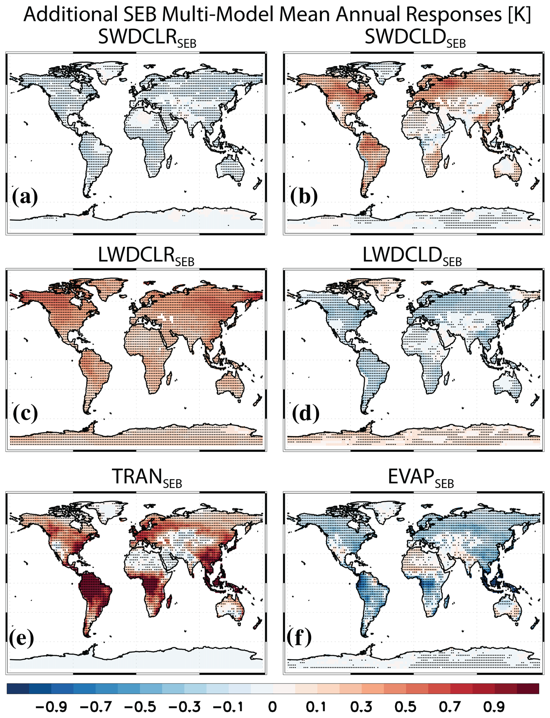
Figure 4 Additional Surface Energy Balance (SEB) decomposition of the surface temperature response. Multimodel mean annual mean SEB PHYS-PI responses for SWD_SEB decomposed into (a) clear-sky (SWDCLR_SEB) and (b) cloudy-sky (SWDCLD_SEB) contributions, LWD_SEB decomposed into (c) clear-sky (LWDCLR_SEB) and (d) cloudy-sky (LWDCLD_SEB) contributions, and LHF_SEB decomposed into (e) TRAN_SEB and (f) EVAP_SEB. Units are K. Symbols denote a response significant at the 90 % confidence level based on a two-tailed pooled t test.

Although all of the SEB terms may contain temperature-induced feedbacks to some extent (since these are coupled ocean–atmosphere simulations), warming associated with LWD_SEB (particularly its clear-sky component) is likely a response to the surface warming as opposed to a driver of the warming. Surface warming will lead to an increase in upwelling LW radiation consistent with the Stefan–Boltzmann law, whereby a blackbody radiates energy proportional to TS⁴. Some of this enhanced upwards longwave radiation (via the atmospheric greenhouse effect) will be reradiated back down to the surface, i.e., enhanced downwelling LW radiation at the surface. This argument is consistent with Vargas Zeppetello et al. (2019), who found surface downwelling LW radiation is tightly coupled to surface temperature. Changes in LWD_SEB are also likely augmented by increases in atmospheric water vapor via the water vapor feedback (i.e., a stronger greenhouse effect). For example, the multimodel global mean tropospheric specific humidity significantly increases by 0.017±0.014 g kg⁻¹. Increases also occur over land at 0.011±0.015 g kg⁻¹, but these are not significant (Table S3; Fig. S6f).

I also note that the SHF_SEB cooling is likely a consequence of the surface warming and the LHF_SEB warming. Surface warming (largely induced by decreases in surface latent heat flux, decreases in surface albedo and increases in solar radiation) will lead to an increase in sensible heat flux, which will act to cool the surface. Similarly, from a Surface Energy Balance standpoint, a reduction in latent heat flux implies an increase in other terms of the Surface Energy Balance, such as sensible heat flux. Spatially correlating the multimodel mean change in SHF_SEB and LHF_SEB yields a very strong global land correlation of −0.90, which increases to −0.92 over tropical land. Similar results exist across models; i.e., the correlation between each model's SHF_SEB and LHF_SEB is −0.84 over global land, which increases to −0.86 over tropical land (correlations are significant at the 99 % confidence level). Thus, these correlations support a strong inverse relationship between SHF_SEB and LHF_SEB. As LHF_SEB leads to warming consistent with reduced stomatal conductance under elevated CO₂, this is also associated with SHF_SEB cooling.

LWD_SEB can be decomposed into clear-sky (LWDCLR_SEB; Fig. 4c) and cloudy-sky (LWDCLD_SEB; Fig. 4d) contributions. All of the multimodel mean global land warming associated with LWD_SEB is due to LWDCLR_SEB at 0.27±0.13 K (12 of 14 models agree on the warming). The dominance of the LWDCLR_SEB warming is consistent with the aforementioned greenhouse effect, combined with increased atmospheric water vapor. In contrast, LWDCLD_SEB contributes to multimodel mean global land cooling of $-\mathrm{0.07}\pm \mathrm{0.03}$ K (12 of 14 models agree on the cooling). This cooling is consistent with a multimodel mean global land decrease in total cloud cover at $-\mathrm{0.52}\pm \mathrm{0.23}$ % (12 of 15 models agree on the decrease; Figs. S6a and S7a). A decrease in cloud cover will act similarly to the greenhouse effect (i.e., here a weaker greenhouse effect), and this will promote a decrease in surface downwelling LW radiation. Consistently, larger multimodel mean LWDCLD_SEB cooling occurs in the extratropics at $-\mathrm{0.11}\pm \mathrm{0.05}$ K, consistent with the larger decrease in extratropical total cloud cover at $-\mathrm{0.64}\pm \mathrm{0.29}$ %.

I note that the multimodel mean decrease in global land cloud cover is consistent with the previously discussed decrease in latent heat flux (largely due to decreases in canopy transpiration) and with decreases in near-surface and tropospheric relative humidity over land (Figs. S6c, d and S7c, d). For example, the multimodel mean global land decrease in near-surface relative humidity is $-\mathrm{0.87}\pm \mathrm{0.48}$ %, which increases in magnitude (as does canopy transpiration) to $-\mathrm{1.09}\pm \mathrm{0.59}$ % over tropical land (11 of 14 models agree on both decreases). The corresponding decrease in multimodel mean global land tropospheric relative humidity is weaker but still significant at $-\mathrm{0.21}\pm \mathrm{0.12}$ % (12 of 14 models agree on the decrease). The near-surface relative humidity decrease over land is consistent with near-surface land warming (which increases the water vapor carrying capacity of the air) and with a (nonsignificant) decrease in near-surface specific humidity ($-\mathrm{0.010}\pm \mathrm{0.052}$ g kg⁻¹; Figs. S6e and S7e). The tropospheric relative humidity decrease over land is consistent with tropospheric warming (0.18±0.09 K) dominating over nonsignificant increases in tropospheric specific humidity (0.011±0.015 g kg⁻¹; Figs. S6f and S7f). I also note a multimodel mean decrease in global land precipitation (Figs. S6b and S7b) at $-\mathrm{0.028}\pm \mathrm{0.017}$ mm d⁻¹ (−1.2 % change relative to the control), with 12 of 15 models agreeing on the decrease.

Warming associated with α_SEB is consistent with surface darkening (e.g., Betts, 2000; Bala et al., 2006; Li et al., 2015) under enhanced vegetation (e.g., LAI increases; Fig. 1b). In contrast to maximum tropical warming due to LHF_SEB, warming associated with α_SEB is largest in the extratropics. The corresponding multimodel mean extratropical land warming is 0.16±0.09 K relative to the tropical warming of 0.06±0.04 K. Larger extratropical as opposed to tropical warming under α_SEB is consistent with larger vegetation-induced darkening over higher latitudes, where snow (i.e., a bright surface with high albedo) is more prevalent (Betts and Ball, 1997; Li et al., 2015). Re-estimating α_SEB by season in the extratropics (which is dominated by the Northern Hemisphere) shows that the dominant warming effect occurs in December thru February and March thru May at 0.26±0.15 and 0.21±0.12 K, respectively. Smaller warming occurs during June thru August and September thru November at 0.07±0.05 and 0.11±0.06 K, respectively. The larger α_SEB warming during the Northern Hemisphere cold months is consistent with the co-occurrence of snow and vegetation.

SWD_SEB yields multimodel mean global land warming of 0.09±0.06 K (12 of 15 models agree on the warming), which can be decomposed into clear-sky (SWDCLR_SEB; Fig. 4a) and cloudy-sky (SWDCLD_SEB; Fig. 4b) contributions. In contrast to SWD_SEB, SWDCLR_SEB yields multimodel mean global land cooling at $-\mathrm{0.05}\pm \mathrm{0.02}$ K. Such cooling is consistent with the aforementioned increase in tropospheric specific humidity, which increases the atmospheric absorption of shortwave radiation by water vapor. Changes in atmospheric aerosols may also contribute though direct scattering/absorption of solar radiation. Few models, however, archived the relevant aerosol diagnostics, and changes in the multimodel mean aerosol optical depth (AOD; Fig. S8) lack significance except for tropical land (Table S3). For example, a nonsignificant multimodel global land AOD increase of $\mathrm{1.88}\pm \mathrm{2.50}\times {\mathrm{10}}^{-\mathrm{3}}$ occurs, with 5 of the 8 models agreeing on the increase. This increases and becomes significant over tropical land at $\mathrm{3.07}\pm \mathrm{3.00}\times {\mathrm{10}}^{-\mathrm{3}}$ (5 of 8 models agree on the increase). Part of these AOD increases are due to (nonsignificant) increases in dust AOD (DAOD; Table S3). If I remove DAOD from (total) AOD (i.e., $\mathrm{AODNOD}=\mathrm{AOD}-\mathrm{DAOD}$), I find nonsignificant AODNOD increases for global and extratropical land but significant increases over tropical land at $\mathrm{2.35}\pm \mathrm{2.33}\times {\mathrm{10}}^{-\mathrm{3}}$ (5 of 8 models agree on this increase).

Of the three models with an interactive representation of BVOCs, only two archived AOD (GFDL-ESM4 and UKESM1-0-LL), and both models yield much larger AOD increases than the other models. Such AOD increases are consistent with enhanced BVOC emissions due to the increased vegetation (e.g., LAI; Fig. 1b), leading to more secondary organic aerosol (SOA) (e.g., Scott et al., 2018; Weber et al., 2024). For example, AOD increases over global land by $\mathrm{7.78}\pm \mathrm{1.00}\times {\mathrm{10}}^{-\mathrm{3}}$ and $\mathrm{7.87}\pm \mathrm{0.78}\times {\mathrm{10}}^{-\mathrm{3}}$ for GFDL-ESM4 and UKESM1-0-LL, respectively (compared to the multimodel mean increase of $\mathrm{1.88}\pm \mathrm{2.50}\times {\mathrm{10}}^{-\mathrm{3}}$). For GFDL-ESM4, a large fraction of this AOD increase is due to an increase in DAOD at $\mathrm{4.82}\pm \mathrm{0.91}\times {\mathrm{10}}^{-\mathrm{3}}$ (UKESM1-0-LL yields a nonsignificant DAOD decrease of $-\mathrm{0.38}\pm \mathrm{0.78}\times {\mathrm{10}}^{-\mathrm{3}}$). Nonetheless, AODNOD (which includes SOA) yields relatively large and significant global land increases for both models at $\mathrm{2.97}\pm \mathrm{0.41}\times {\mathrm{10}}^{-\mathrm{3}}$ for GFDL-ESM4 and $\mathrm{8.26}\pm \mathrm{0.38}\times {\mathrm{10}}^{-\mathrm{3}}$ for UKESM1-0-LL (Fig. S8g–h). These values increase over tropical land (where vegetation indices also increase the most) at $\mathrm{6.16}\pm \mathrm{0.85}\times {\mathrm{10}}^{-\mathrm{3}}$ and $\mathrm{10.68}\pm \mathrm{0.63}\times {\mathrm{10}}^{-\mathrm{3}}$ for GFDL-ESM4 and UKESM1-0-LL, respectively. In turn, both models feature SWDCLR_SEB cooling (consistent with enhanced aerosol scattering) over global land (and over tropical and extratropical land) of $-\mathrm{0.13}\pm \mathrm{0.02}$ for GFDL-ESM4 and $-\mathrm{0.07}\pm \mathrm{0.02}$ K for UKESM1-0-LL (compared to the multimodel mean of $-\mathrm{0.05}\pm \mathrm{0.02}$ K). NorESM2-LM, the other model with an interactive representation of BVOCs (but no AOD data), also yields relatively large SWDCLR_SEB cooling at $-\mathrm{0.08}\pm \mathrm{0.03}$ K. The GFDL-ESM4 SWDCLR_SEB cooling is the second largest of the 15 models; the NorESM2-LM and UKESM1-0-LL SWDCLR_SEB cooling are third and fourth largest, respectively. Similar statements also generally apply for tropical land; e.g., the NorESM2-LM SWDCLR_SEB cooling of $-\mathrm{0.16}\pm \mathrm{0.05}$ K is the largest, and the GFDL-ESM4 SWDCLR_SEB cooling of $-\mathrm{0.11}\pm \mathrm{0.03}$ K is the third largest. However, UKESM1-0-LL SWDCLR_SEB cooling is not exceptional at $-\mathrm{0.04}\pm \mathrm{0.04}$ K (compared to the multimodel mean of $-\mathrm{0.05}\pm \mathrm{0.02}$ K). Thus, consistent with Gomez et al. (2023), there is evidence that models with interactive chemistry yield AOD increases under carbon fertilization, consistent with enhanced vegetation leading to more BVOC emissions and SOA. In turn, this appears to strengthen the cooling associated with the SWDCLR_SEB (with enhanced water vapor and reduced surface solar radiation also contributing). I also note that the AOD increase here is also consistent with the land–sea warming contrast (e.g., Fig. 2a) and reduced precipitation over land (Fig. S6b), which leads to less aerosol wet removal (Allen et al., 2019).

As SWDCLR_SEB term leads to multimodel mean cooling, the warming under SWD_SEB is therefore associated with clouds. SWDCLD_SEB yields multimodel mean global land warming of 0.14±0.05 K (12 of 15 models agree on the increase), which increases to 0.21±0.08 K over extratropical land. As with the LWDCLD_SEB cooling, this SWDCLD_SEB warming is consistent with decreases in cloud cover (e.g., here, less cloud cover will lead to enhanced surface solar radiation and warming). Moreover, both LWDCLD_SEB and SWDCLD_SEB are largest in magnitude in the extratropics, consistent with larger extratropical cloud cover decrease. I note that the net effect of clouds is controlled by their impact on shortwave as opposed to longwave radiation. SWDCLD_SEB yields multimodel global land mean warming of 0.14±0.05 K, while the LWDCLD_SEB yields corresponding cooling of $-\mathrm{0.07}\pm \mathrm{0.03}$ K. This implies that the net effect of clouds is associated with warming of 0.07±0.06 K. The net warming effect from clouds increases over extratropical land at 0.10±0.09 K.

I also note that I do not find evidence for an aerosol indirect effect on clouds and in turn SWDCLD_SEB. As discussed above, the two models with interactive chemistry simulate relatively large and significant increases in AODNOD, particularly over tropical land (which potentially leads to SWDCLD_SEB cooling related to cloud brightening and enhanced cloud lifetime). However, as with the multimodel mean, SWDCLD_SEB leads to warming over global land, tropical land and extratropical land for both models (as well as NorESM2-LM). UKESM1-0-LL actually yields the largest SWDCLD_SEB warming of the 15 models over both global land and tropical land at 0.32±0.02 and 0.28±0.05 K, respectively. In contrast to an aerosol indirect effect, this SWDCLD_SEB warming in UKESM1-0-LL is consistent with a decrease in cloud cover, as UKESM1-0-LL yields the second largest cloud cover decrease over global land at $-\mathrm{1.35}\pm \mathrm{0.14}$ % and the third largest decrease over tropical land at $-\mathrm{1.20}\pm \mathrm{0.29}$ %. Overall, (total) SWD_SEB warms global land in UKESM1-0-LL and NorESM2-LM by 0.25±0.03 and 0.10±0.05 K, respectively, with nonsignificant cooling of $-\mathrm{0.02}\pm \mathrm{0.02}$ K for GFDL-ESM4. Thus, as with the multimodel mean results, SWDCLD_SEB warming dominates over SWDCLR_SEB cooling in these three models. Any impacts of interactive chemistry and enhanced BVOC emissions/SOA on clouds appear to be minor in these simulations and do not lead to an appreciable increase in cooling.

I note that semi-arid regions, such as the southwest US and parts of western and central Asia, show SEB changes that are in general opposite those at similar latitudes (Figs. 3 and 4). In the southwest US, for example, there is cooling associated with both SWD_SEB (in part related to increased cloud cover; Figs. S6–S7) and LHF_SEB (due to increased transpiration), as well as relatively large warming associated with α_SEB. The region also shows an increase in near-surface and tropospheric relative humidity (Figs. S6–S7). This is consistent with the different behavior in water-limited regions relative to energy-limited regions; i.e., carbon fertilization in water-limited regions is expected to yield larger (relative) increases in photosynthesis and vegetation indices (Donohue et al., 2013). Consistently, I find a relatively large increase in the percent change in LAI for the southwest US (not shown). This in turn supports the relatively large surface darkening (warming under α_SEB) and increases in canopy transpiration and cloud cover.

Spatially correlating the multimodel mean SEB responses with the corresponding total SEB (Total_SEB) response yields significant global (land only) correlations for all individual SEB terms (Table S5). Consistent with the sign of the multimodel mean SEB responses, Total_SEB is positively correlated with α_SEB, SWD_SEB, SWDCLD_SEB, LWD_SEB, LWDCLR_SEB, LHF_SEB and TRAN_SEB. Similarly, Total_SEB is negatively correlated with SWDCLR_SEB, LWDCLD_SEB, SHF_SEB and EVAP_SEB. The LWDCLR_SEB term yields the largest global correlation with Total_SEB at 0.91. Restricting this analysis to the tropics yields maximum correlations between Total_SEB and LHF_SEB at 0.77, followed closely by the LWDCLR_SEB at 0.76. This provides additional support for the importance of the multimodel mean LHF_SEB response to Total_SEB in the tropics. In the extratropics, maximum correlations occur for LWDCLR_SEB at 0.90, followed by LWD_SEB at 0.58 and SWDCLD_SEB at 0.57.

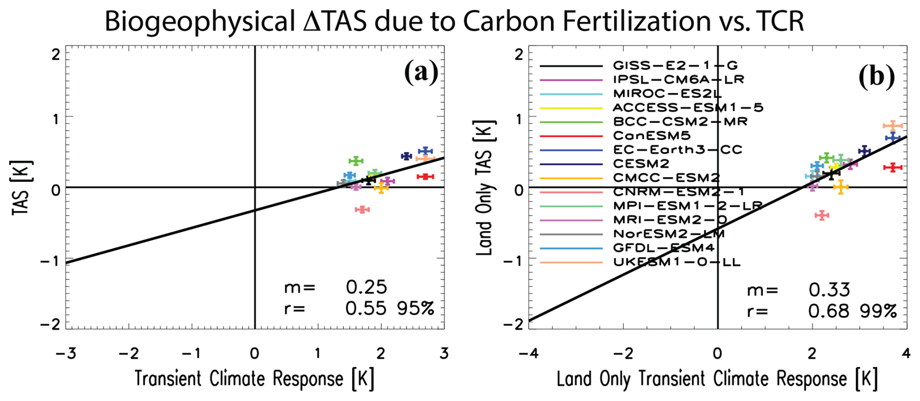
Figure 5 Scatter plots of the global mean near-surface temperature response versus the transient climate response across models. Scatter plots between the (a) global mean near-surface air temperature PHYS-PI response (TAS, y axis) and the transient climate response (TCR). Panel (b) is analogous but for land only. Each symbol represents an individual model (see legend). Error bars for each symbol represent the 90 % confidence intervals based on a two-tailed pooled t test. Black line represents the least-squares linear regression line. The corresponding slope (m) of the regression and the correlation coefficient (r) are included. Significant correlations based on a two-tailed test at the 95 % and 99 % confidence level are indicated. Units are K.

I conduct additional analyses to better understand causes of inter-model spread in the SEB responses. Figures S9 and S10 shows spatial correlations (across models) between Total_SEB and each of the SEB components. LWD_SEB shows very large and significant correlations (r>0.80) throughout most of the Northern Hemisphere (NH), with nearly all land areas exhibiting similarly large and significant correlations under LWDCLR_SEB. LHF_SEB shows relatively large and significant positive correlations (r>0.70) throughout the tropics (minus the Sahara Desert). α_SEB shows relatively large and significant positive correlations (r>0.70) in the NH extratropics. This suggests much of the intermodel variation in the Total_SEB extratropical surface temperature response is related to intermodel differences in the α_SEB response; in the tropics, intermodel variation in the Total_SEB tropical surface temperature response is related to intermodel differences in the LHF_SEB response. Additional discussion of intermodel differences is included in the Supplement (Sect. S1).

Finally, I note a correlation of 0.55 (significant at the 95 % confidence level; Fig. 5) between the transient climate response (TCR; warming centered on the time of CO₂ doubling) and the global mean biogeophysical temperature response associated with carbon fertilization across models. The correlation improves to 0.68 (significant at the 99 % confidence level) over global land only (Fig. 5b). Such a relationship is consistent with the findings of Zarakas et al. (2020), who showed the physiological effect contributes 6.1 % to the full TCR and that the variation in the physiological contribution to the TCR across models contributes disproportionately more to the intermodel spread of TCR than it does to the mean. In particular, the three models (EC-Earth3-CC, UKESM1-0-LL and CESM2) mentioned above that yield the largest biogeophysical warming associated with carbon fertilization are among the models with the largest TCR (CanESM5 is an exception at it has a large TCR but relatively small biogeophysical warming). On one hand, this correlation may imply the possible importance of the biogeophysical warming associated with the carbon fertilization effect to intermodel variation in the TCR (e.g., via climate feedbacks including water vapor, tropospheric lapse rate, surface albedo and clouds). I note, however, that this correlation is not particularly large and is heavily influenced by the three aforementioned models (e.g., removing the three models with large TCR and biogeophysical warming reduces the land-only correlation to 0.30). Furthermore, the magnitude of biogeophysical warming associated with carbon fertilization is relatively small. If I re-estimate the global mean near-surface air temperature response over the time of CO₂ doubling (years 60–79, as with TCR), I find biogeophysical warming of 0.12±0.08 K, i.e., about 6 % as large as the multimodel mean TCR of 1.97±0.20 K. However, some models yield much larger biogeophysical warming at the time of CO₂ doubling, including many of the same models previously discussed. EC-Earth3-CC yields warming of 0.26±0.05 K, which is 10 % of its TCR of 2.7±0.10 K. CESM2 yields warming of 0.49±0.07 K, which is 20 % of its TCR of 2.4±0.07 K. UKESM1-0-LL yields a percentage closer to the multimodel mean, with warming of 0.19±0.07 K, which is 7 % of its TCR of 2.7±0.14 K.

3.4 Biogeochemical and biogeophysical responses under a warmer background climate

The primary analyses discussed above are repeated, but here the carbon fertilization effect is quantified under a warmer background climate (i.e., FULL-RAD). This is compared to the previous signal under a preindustrial background climate (i.e., PHYS-PI) using the 13 models in common for all four simulations (some variables have less than 13 models available). Figure 6 shows bar charts of the land carbon responses for the globe (Fig. 6a), tropics (Fig. 6b) and extratropics (Fig. 6c) under FULL-RAD, PHYS-PI and the influence of the carbon fertilization effect within the context of a warmer climate, i.e., the double difference (FULL-RAD) − (PHYS-PI). Although all three land carbon pools increase under both FULL-RAD and PHYS-PI, there are some notable differences. Globally, for example, litter and soil carbon increase more under PHYS-PI than under FULL-RAD; i.e., both carbon pools decrease under (FULL-RAD) − (PHYS-PI) at $-\mathrm{13.2}\pm \mathrm{12.2}$ Pg C for litter carbon and (not significant) $-\mathrm{8.5}\pm \mathrm{41.1}$ Pg C for soil organic matter. The weaker increase in these two carbon pools under FULL-RAD is related to the warmer background climate (globally, RAD is 3.75±0.38 K warmer than PI), which increases decomposition of organic matter (Crowther et al., 2016; Bradford et al., 2016; Melillo et al., 2017; Nottingham et al., 2020). In contrast, global vegetation carbon increases more under FULL-RAD than under PHYS-PI; i.e., (FULL-RAD) − (PHYS-PI) yields an increase of 52.8±34.9 Pg C. This vegetation carbon increase is slightly larger in the extratropics as opposed to the tropics at 24.8±13.9 Pg C vs. 22.9±21.6 Pg C. In terms of the change in vegetation carbon density (Table S6), the increase is more pronounced in the extratropics at 0.40±0.22 kg C m⁻² (11 of 12 models agree on the increase) versus 0.26±0.25 kg C m⁻² in the tropics (9 of 12 models agree on the increase). Similar statements apply for both NPP and LAI, both of which yield net increases under (FULL-RAD) − (PHYS-PI), and both yield larger net increases in the extratropics as opposed to the tropics (Table S6). This extratropical versus tropical difference is related to net decreases in most vegetation indices (e.g., NPP and vegetation carbon) under (FULL-RAD) − (PHYS-PI) throughout much of the Amazon, as well as parts of southern Africa and Australia (Fig. S11), which is consistent with a warmer and drier background climate (Nobre and Borma, 2009; Nobre et al., 2016; del Rosario Uribe et al., 2023; Flores et al., 2024). This is also related to enhanced vegetation indices in the NH extratropics, consistent with the notion that warming and a longer growing season may drive an increase in NH high-latitude biomass (Innes, 1991; Kauppi et al., 2014; D'Orangeville et al., 2016; Schaphoff et al., 2016).

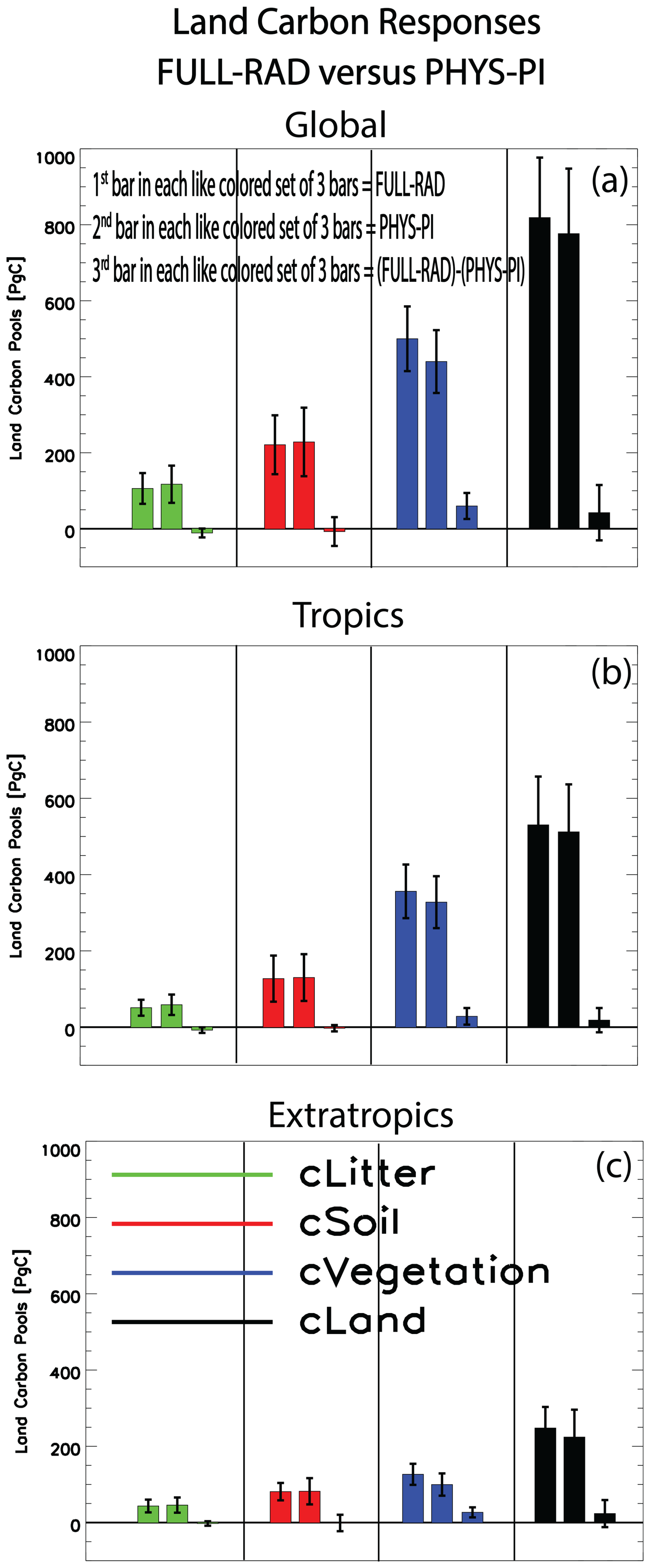
Figure 6 Bar chart of vegetation and land carbon responses. Multimodel mean litter pool carbon (cLitter; green), soil pool carbon (cSoil; red), vegetation carbon (cVegetation; blue) and total land carbon (cLand; black) responses for the (a) globe, (b) tropics and (c) extratropics. Responses are shown for FULL-RAD (first bar in each like-colored set of 3 bars) and PHYS-PI (second bar in each like-colored set of 3 bars). The influence of the carbon fertilization effect within the context of a warmer climate, i.e., (FULL-RAD) − (PHYS-PI), is shown as the third bar in each like-colored set of 3 bars. Error bars show the 90 % confidence level based on individual model responses. Units are Pg C.

Consistent with the relatively large increase in vegetation carbon, total land carbon (the sum of the three pools) also yields a net increase under (FULL-RAD) − (PHYS-PI), with a larger extratropical versus tropical increase (but not significantly so). For example, the global net increase in total land carbon is 32.2±77.1 Pg C, including 19.4±37.9 Pg C in the extratropics versus 12.8±33.2 Pg C in the tropics. Using the TCRE to estimate the corresponding biogeochemical cooling effect yields a relatively small value of 0.05 K (0.03 to 0.07 K). Thus, the overall impact of the warmer background climate on land carbon storage and the biogeochemical cooling effect associated with carbon fertilization is relatively weak cooling.

Figure 7a shows the (biogeophysical) near-surface air temperature response under FULL-RAD. As with PHYS-PI (Fig. 2), significant warming occurs in most regions. (FULL-RAD) − (PHYS-PI) (Fig. 7c) yields net (nonsignificant) global mean warming of 0.05±0.08 K (9/13 models agree), and there are opposing hemispheric responses, with net warming in the NH and net cooling in the Southern Hemisphere (SH). Although (FULL-RAD) − (PHYS-PI) is less robust across models (Fig. 7d), the extratropical land warming (which is largely a NH extratropical signal) is significant at 0.12±0.11 K with 10 of the 13 models agreeing. The global land and tropical land signals are not significant at 0.07±0.09 and $-\mathrm{0.03}\pm \mathrm{0.09}$ K, respectively (7 of the 13 models agree in both cases).

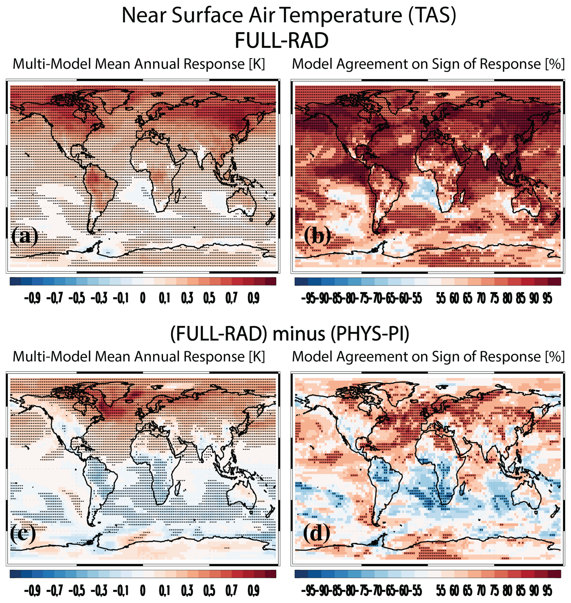
Figure 7 Near-surface air temperature. Multimodel mean annual mean near-surface air temperature (TAS; K) response under (a) FULL-RAD and (c) the influence of the carbon fertilization effect within the context of a warmer climate, i.e., (FULL-RAD) − (PHYS-PI). Symbols denote a response significant at the 90 % confidence level based on a two-tailed pooled t test. Model agreement on the sign of the TAS response [% of models] under (b) FULL-RAD and (d) (FULL-RAD) − (PHYS-PI). Red (blue) colors indicate model agreement on an increase (decrease). Symbols represent significant model agreement at the 90 % confidence level based on a two-tailed binomial test.

The SEB decomposition is again used to understand the drivers of the surface temperature response. Figure 8 shows bar charts of the SEB terms for the global, tropical and extratropical land for FULL-RAD, PHYS-PI and (FULL-RAD) − (PHYS-PI) (spatial maps are included in Figs. S12 and S13). In general, the sign of each SEB term is similar between both FULL-RAD and PHYS-PI; however some notable differences in magnitude exist. Figure 8a suggests the enhanced (nonsignificant) global mean land warming under (FULL-RAD) − (PHYS-PI) is largely related to enhanced warming from LWD_SEB at 0.13±0.11 K (8 of 13 models agree), which is essentially due to LWDCLR_SEB at 0.13±0.12 K (7 of 10 models agree). This response is consistent with the stronger greenhouse effect under the warmer, higher atmospheric CO₂ climate. As argued above, LWD_SEB is largely a response to the surface temperature change, so this implies the FULL-RAD warming due to the other SEB terms (e.g., α_SEB, SWD_SEB, and TRANS_SEB) is magnified via the enhanced greenhouse effect. SHF_SEB also contributes to net warming at 0.06±0.03 K (9 of 13 models agree), which as argued above is likely associated with the change in LHF_SEB, which yields net cooling at $-\mathrm{0.10}\pm \mathrm{0.03}$ K (13 of 13 models agree). LHF_SEB cooling is largely due to TRAN_SEB at $-\mathrm{0.17}\pm \mathrm{0.04}$ K (11 of 11 models agree), which is weakened by EVAP_SEB warming at 0.06±0.04 K (9 of 11 models agree). The net increase in LHF and canopy transpiration under (FULL-RAD) − (PHYS-PI) is related to the warmer temperatures and higher evaporative demand of the atmosphere (Sherwood and Fu, 2014). It is also generally consistent with the net increase in LAI (Fig. S11). Net cooling under (FULL-RAD) − (PHYS-PI) also occurs for SWD_SEB at $-\mathrm{0.021}\pm \mathrm{0.020}$ K (8 of 13 models agree), largely associated with SWDCLD_SEB at $-\mathrm{0.019}\pm \mathrm{0.021}$ K (9 of 12 models agree). This effect is also related to the increase in transpiration, which (as discussed above) increases near-surface and tropospheric relative humidity and promotes cloud cover, which reflects more incoming sunlight. α_SEB contributes nonsignificant cooling at $-\mathrm{0.015}\pm \mathrm{0.027}$ K (8 of 13 models agree). The larger increase in LAI under (FULL-RAD) − (PHYS-PI) (Fig. S11) should promote more surface darkening, but this appears to be offset by less snow over land under a warmer background climate, effectively weakening the surface darkening effect.

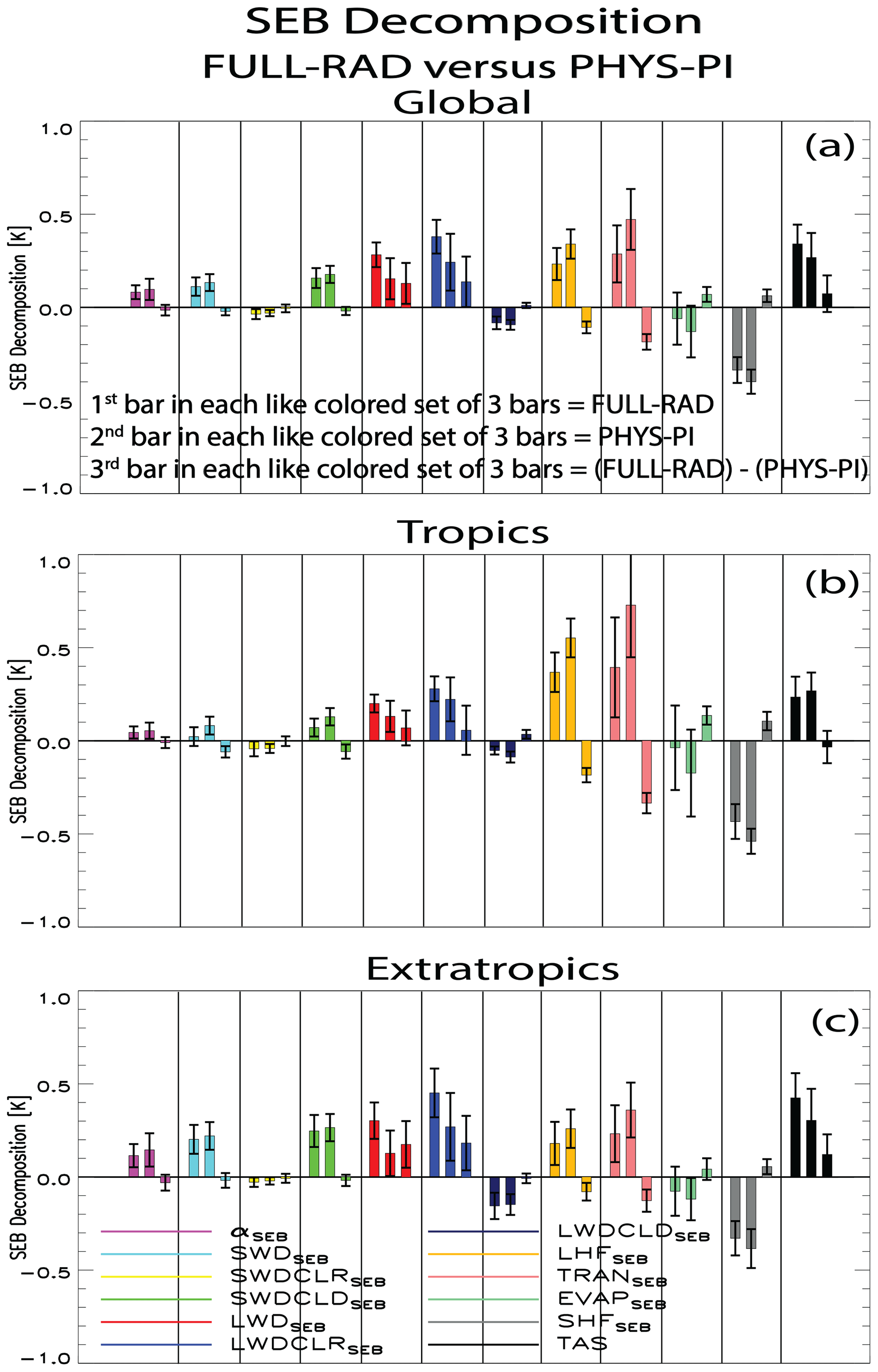
Figure 8 Surface energy balance (SEB) decomposition of the surface temperature response. Annual mean SEB responses for the (a) globe, (b) tropics and (c) extratropics. SEB terms include α_SEB (purple); SWD_SEB (cyan) and its clear-sky (SWDCLR_SEB; yellow) and cloudy-sky (SWDCLD_SEB; bright green) contributions, LWD_SEB (red) and its clear-sky (LWDCLR_SEB; blue) and cloudy-sky (LWDCLD_SEB; navy) contributions, LHF_SEB (orange) and its transpiration (TRAN_SEB; pink) and evaporation (EVAP_SEB; darker green) components, SHF_SEB (gray), and near-surface air temperature (TAS; black). Responses are shown for FULL-RAD (first bar in each like-colored set of 3 bars) and PHYS-PI (second bar in each like-colored set of 3 bars). The influence of the carbon fertilization effect within the context of a warmer climate (FULL-RAD minus PHYS-PI) is shown as the third bar in each like-colored set of 3 bars. Error bars show the 90 % confidence level based on individual model responses. Units are K.

These arguments also apply to the extratropical SEB analysis (Fig. 8c), where the near-surface air temperature over land shows significant warming under (FULL-RAD) − (PHYS-PI) at 0.12±0.11 K (10 of 13 models agree). As with the global mean, the two dominant SEB terms are LWD_SEB and LHF_SEB. Here, the LWD_SEB response (which is again is due to LWDCLR_SEB) under the warmer background climate is more than twice as large as that under the preindustrial background climate, resulting in (FULL-RAD) − (PHYS-PI) warming of 16±0.12 K (9 of 13 models agree). LHF_SEB cooling is weaker at $-\mathrm{0.07}\pm \mathrm{0.05}$ K (9 of 13 models agree), which is again due to TRAN_SEB at $-\mathrm{0.12}\pm \mathrm{0.06}$ K (11 of 11 models agree). Thus, the net increase in extratropical near-surface air temperature under (FULL-RAD) − (PHYS-PI) is due to the enhanced greenhouse effect, which outweighs cooling from increased transpiration.

I note that the above extratropical (largely NH extratropical, 30–60° N) warming under (FULL-RAD) − (PHYS-PI) is amplified farther poleward (>60° N; Fig. S14). Here, land warming is 0.36±0.27 K (10 of 13 models agree). This is due to LWD_SEB (mostly LWDCLR_SEB) at 0.28±0.26 K (10 of 13 models agree) and SWD_SEB (mostly SWDCLD_SEB) at 0.08±0.05 K (10 of 13 models agree). LHF_SEB also yields (nonsignificant) warming at 0.02±0.06 K (7 of 13 models agree), which is due to TRAN_SEB warming (opposite the cooling that occurs everywhere else, e.g., Fig. S13e) at 0.07±0.06 K (8 of 11 models agree). This decrease in NH high-latitude transpiration under (FULL-RAD) − (PHYS-PI) implies a stronger decrease in stomatal conductance, which may be related to the relatively large amount of NH high-latitude vegetation in a warmer world. For example, NH high-latitude NPP and LAI increase by 45.9 % (13/13 models agree) and 31.1 % (12/13 models agree) in RAD relative to PI.

In the tropics (Fig. 8b), nonsignificant net cooling of $-\mathrm{0.03}\pm \mathrm{0.09}$ K occurs under the CO₂ effect, with 7 of the 13 models agreeing. The dominant driver of this cooling is a relatively large net decrease in LHF_SEB at $-\mathrm{0.18}\pm \mathrm{0.04}$ K (13 of 13 models agree), which is again due to a relatively large decrease in TRAN_SEB at $-\mathrm{0.31}\pm \mathrm{0.05}$ K (11 of 11 models agree). SWD_SEB also contributes at $-\mathrm{0.06}\pm \mathrm{0.03}$ K (11 of 13 models agree), which is largely due to SWDCLD_SEB at $-\mathrm{0.06}\pm \mathrm{0.04}$ K (8 of 12 models agree). As mentioned above, this is likely a consequence of the increase in transpiration and, in turn, tropospheric relative humidity and cloud cover. In contrast, LWD_SEB yields relatively small (and not significant) net warming of .07±0.09 K (9 of 13 models agree). Thus, the (nonsignificant) net decrease in tropical near-surface air temperature under (FULL-RAD) − (PHYS-PI) is due to enhanced cooling from increased transpiration, which outweighs warming from increased downwelling longwave radiation.

Finally, I note that the FULL-RAD near-surface air temperature response yields a significant intermodel correlation with TCR, similar to PHYS-PI (Fig. 5). Here, the correlation is 0.66 for land only and 0.60 over land and ocean (both significant at the 95 % confidence level; Fig. S15). Again, however, this relationship is heavily influenced by a handful of models that yield relatively large values for both ΔTAS and TCR (e.g., UKESM1-0-LL and CanESM5).

4 Conclusions

Using a relatively large number of CMIP6 climate models (up to 15), I show that carbon fertilization under a preindustrial background climate (PHYS-PI) at the time of CO₂ quadrupling (and in the absence of radiative warming from CO₂) yields biogeophysical global mean warming of 0.16±0.09 K, with 13 of the 15 models yielding warming. This warming increases over global land to 0.28±0.13 K, with 14 of the 15 models yielding warming (Table S4). Such warming is qualitatively consistent with prior studies on this topic (Sellers et al., 1996; Boucher et al., 2009; Cao et al., 2010; Arora et al., 2013; Arora et al., 2020; Zarakas et al., 2020). As expected, this warming is also very similar to that in Zarakas et al. (2020), who found model mean warming of 0.14 K (standard deviation of 0.16 K) in 12 CMIP6 models.

As mentioned in the Introduction, one of the main novelties of this analysis is the use of the Surface Energy Balance decomposition to systematically quantify the drivers of the warming associated with carbon fertilization. This decomposition shows that the warming is largely related to decreased latent heat flux, which leads to global land warming of 0.27±0.11 K (13 of 15 models agree on the warming). This in turn is largely associated with reduced canopy transpiration, which leads to global land warming of 0.45±0.15 (13 of 13 models agree on the warming). Such a response is consistent with reduced stomatal conductance under elevated CO₂ (e.g., Wong et al., 1979; Keenan et al., 2013). To some extent, this warming if offset by increases in evaporation, which leads to global land cooling of $-\mathrm{0.19}\pm \mathrm{0.16}$ K. This cooling, however, is less robustly simulated with only 9 of the 13 models agreeing on the cooling. In the tropics, the importance of transpiration-induced warming increases to 0.70±0.26 K (13/13 models agree). Tropical land evaporation increases only marginally to $-\mathrm{0.26}\pm \mathrm{0.25}$ K but with limited model agreement (7/13 models agree on the cooling). Of the various SEB terms, the evaporation term is the most uncertain across the models (particularly in the tropics), with limited model agreement on the sign of the response. Given the importance of latent heat flux to the biogeophysical warming response (both its direct impact and its indirect impact on clouds) and the competing effects of transpiration versus evaporation, the low model agreement on the sign of the evaporation response highlights an important source of model uncertainty.

Other important drivers of biogeophysical warming under carbon fertilization, particularly in the extratropics, include reduced albedo and enhanced SW radiation due to a decrease in cloud cover. Warming due to reduced albedo is consistent with the surface darkening effect of vegetation (e.g., Betts, 2000; Bala et al., 2006; Li et al., 2015), particularly at higher latitudes where snow/ice is more prevalent. Warming due to enhanced shortwave radiation due to clouds is consistent with decreases in total cloud cover. This is consistent with the HadCM3LC version of the Met Office Unified Model System used by Doutriaux-Boucher et al. (2009). Similar to the decrease in latent heat flux, the decrease in cloud cover is related to the reduced stomatal conductance, which is associated with reduced relative humidity over land which promotes a decrease in cloud cover. Another novelty of this study is the investigation of the vegetation–aerosol response to carbon fertilization under increasing CO₂. Models with interactive BVOCs (unfortunately this includes only 3 models) yield a larger increase in AOD, which strengthens the cooling associated with the SW_clear; however, as with the multimodel mean, SW_cloud warming dominates over SW_clear cooling in these models, implying any aerosol effect is minor in these simulations (i.e., the dominant SW effect is warming due to cloud cover reductions associated with decreases in transpiration).

Intermodel variation in the vegetation and biogeophysical temperature responses was also evaluated. Although there are significant differences between models with and without a terrestrial nitrogen cycle (e.g., N models yield significantly less carbon storage), most of these differences (e.g., N models tend to yield less biogeochemical cooling) are not significant. Consistent with Zarakas et al. (2020), intermodel biogeophysical warming significantly correlates with each model's TCR. This implies the causes of intermodel TCR variation (i.e., climate feedbacks) are also responsible for some of the intermodel spread in the biogeophysical temperature response under carbon fertilization. Finally, the increase in land carbon storage under carbon fertilization was used to estimate the biogeochemical cooling effect using the transient climate response to cumulative emissions. I find that biogeochemical cooling of −1.38 K (−1.92 to −0.84 K) dominates over biogeophysical warming, by about an order of magnitude.

Another novelty of the present study is quantification of the carbon fertilization effect under two different background climates. Although analogous simulations (FULL-RAD) that isolate the CO₂ fertilization effect under a warmer background climate yield similar overall results, they indicate stronger (relative to PHYS-PI) biogeophysical warming of the extratropical land (largely in the NH) at 0.12±0.11 K (10/13 models agree) but weaker (and not significant) warming of tropical land at $-\mathrm{0.03}\pm \mathrm{0.09}$ K (7/13 models agree). The former is related to relatively large LWD_SEB warming, consistent with the stronger greenhouse effect under the warmer, higher atmospheric CO₂ climate. The latter is related to relatively large net cooling from smaller decreases (i.e., net increases) in transpiration, consistent with higher evaporative demand of the atmosphere under the warmer, higher atmospheric CO₂ climate. In addition, larger but nonsignificant increases in land carbon storage occur under the warmer background climate, implying a small increase in the biogeochemical cooling effect of −0.05 (−0.03 to −0.07 K). This is, however, essentially equal in magnitude to the net biogeophysical global mean warming of .05±0.08 K (9/13 models agree). Thus, there is no change in the total (biogeochemical + biogeophysical) near-surface air temperature response under the two background climates, i.e., (FULL-RAD) versus (PHYS-PI). The climate effects of carbon fertilization are therefore relatively robust across the two different background climates.