Origin, size distribution, and hygroscopic properties of marine aerosols in the southwestern Indian Ocean: results of six campaigns of shipborne observations

This study presents observations of marine aerosols made during six ship-based campaigns in the southwestern Indian Ocean in 2021 and 2023. A set of aerosol measurement instruments is used to study the spatial and temporal variability in the number and size distribution of marine aerosols, the concentration of cloud condensation nuclei (CCN), and the hygroscopic properties of aerosols (kappa–Köhler parameter, κ). It has been shown that the number of submicron aerosols measured varies much more significantly (ranging from 100 to over 3000 cm⁻³) than the number of CCN (60 to 500 cm⁻³ at 0.4 % supersaturation). As a result, the κ values obtained show considerable variability, ranging from 0.05 to 0.7. Four distinct scenarios are examined to elucidate some of these variations: (1) the predominance of pristine air masses in the eastern regions of the subtropical Indian Ocean, with highly variable κ values sensitive to the low aerosol concentration measured in this area; (2) the predominance of polluted air masses in the Mozambique Channel, with weakly hydrophilic aerosols; (3) a precipitation and storm event in the southern Indian Ocean, with highly variable κ values; and (4) a new particle formation event in the open ocean, with an increase in κ values as the newly formed particles grow to Aitken mode particles.

The size distribution of the sampled marine aerosols was analyzed according to the origin of the air masses. In general, a shift of the Aitken and accumulation modes toward larger aerosol sizes was observed for continental and subtropical air masses in the Indian Ocean due to aging. Conversely, the modes shifted toward smaller sizes for air masses in the southern Indian Ocean due to higher primary marine emissions. Aerosols are more hydrophobic for continental air masses (κ ∼ 0.1), more hydrophilic and variable over the subtropical Indian Ocean (κ ranging from 0.2 to 0.6), and intermediate (κ ∼ 0.2) over the southern Indian Ocean. The κ of the subtropical Indian Ocean increases with wind intensity, while it remains stable in the southern Indian Ocean. This effect is attributed to the high proportion of primary organic matter, which is due to the important concentration of nanophytoplankton in the southern Indian Ocean. It has been shown that primary organic aerosols act as surfactants, thus counterbalancing the highly hydrophilic properties of NaCl.

1 Introduction

Aerosols have been identified as playing a key role in climate, cloud formation, and cloud lifetime through their direct and indirect effects (IPCC, 2013, 2021; Wall et al., 2023). Among them, marine aerosols constitute a significant mass proportion of particles, with global emissions estimated between 2000 and 10 000 Tg yr⁻¹ (O'Dowd et al., 1997; Bates et al., 2005; Textor et al., 2006; de Leeuw et al., 2011). Marine aerosols are defined as aerosols comprising all types of particles found over the oceans, regardless of their point of origin. Some come from local sources and are mechanically injected into the atmosphere via either bubble bursting (Lewis and Schwartz, 2004; de Leeuw et al., 2011) or wave crest tearing (Monahan et al., 1986) or are chemically formed by gas to particle conversion after gas emission from the ocean, essentially due to phytoplankton activity (Saltzman, 2009; de Leeuw et al., 2014). Others come from remote sources and are transported from landmasses toward the ocean as dust (Schulz et al., 2012), biomass burning aerosols, or particles originating from fossil fuel combustion (Ramanathan et al., 2001; Novakov et al., 2000). This diversity of origins makes the size and chemical composition of marine aerosols highly variable. These two characteristics are essential in determining aerosol hygroscopicity, which is the ability of aerosols to take up the surrounding atmospheric water vapor and grow to larger sizes. Thus, according to their hygroscopicity, marine aerosols may act as cloud condensation nuclei (CCN) and activate as cloud droplets, leading to cloud formation (Köhler, 1936). Clouds, in turn, affect the Earth's energy balance by reflecting shortwave radiation and absorbing and emitting longwave radiation. Indeed, a change in aerosol concentration or its properties affects cloud droplet number concentration (Twomey, 1974, 1977) and cloud lifetime, leading to changes in precipitation (Albrecht, 1989). For instance, low clouds, such as marine stratocumulus, which is the most widely spread cloud type on Earth (Warren et al., 1988, 2007), have been intensively studied due to their strong sensitivity to aerosol concentration changes, which affect their cloud droplet number (Stevens et al., 1998; Sandu et al., 2008; Brioude et al., 2009; Jia et al., 2019). Therefore, the complex interactions between aerosols and these clouds in the marine environment constitute one of the largest uncertainties in climate models (Carslaw et al., 2013; Simpkins, 2018) and contribute to less accurate climate predictions. One of the primary reasons for these uncertainties lies in the inadequate depiction of aerosol sources in the remote marine ocean (Carslaw et al., 2017). In this region, where aerosol loads are the lowest, cloud droplet sensitivities are the greatest (Moore et al., 2013).

To improve our understanding of the life cycle, size distribution, and chemical composition of marine aerosols and their impact on climate, several studies have been conducted mainly in the Atlantic, Pacific, and northern Indian oceans (Heintzenberg et al., 2000). Some studies focused on the physical properties of marine aerosols and reported a wide range of number concentrations associated with a variable size distribution. For instance, Flores et al. (2020) measured strong differences in aerosol number concentrations, with an average of 180 ± 51 cm⁻³ in the Pacific Ocean and 864 ± 806 cm⁻³ in the Atlantic Ocean. Under the influence of an air mass of continental origin, the number of aerosols can reach several thousand particles per cm⁻³ (Flores et al., 2020).

Other studies have focused on the variability in aerosol chemical composition. For instance, Yoon et al. (2007) investigated the seasonal chemical composition of marine aerosols in the North Atlantic Ocean and found a maximum mass concentration of NaCl in the coarse mode during winter due to stronger wind speeds during this season. In contrast, they measured a higher sulfate concentration in summer than in winter in the submicrometer mode. In the eastern part of the Atlantic Ocean, O'Dowd et al. (2004) and Cavalli et al. (2004) observed a significant fraction of organic matter in primary marine aerosols, which they explained by the presence of phytoplankton blooms. During a phytoplankton bloom, Facchini et al. (2008) observed an increase in the organic fraction of primary marine aerosols from 3 % to 77 %, while the diameter of the particles decreased from 8 µm to 125 nm. On Amsterdam Island, during summer, Sciare et al. (2009) also observed a peak in the organic fraction of primary marine aerosols (> 250 ng m⁻³), which they related to a region with a high concentration of Chlorophyll a located between 1000 and 2000 km from the measurement site. Sciare et al. (2009) also observed a higher concentration of black carbon in marine aerosols during winter (7–13 ng m⁻³) than during summer (2–5 ng m⁻³). They explained this increase in the black carbon fraction by the transport of pollution plumes from South Africa and Madagascar (fires and combustion of fossil fuels).

Other studies focused on CCN number concentration. In the Southern Ocean, Quinn et al. (2017) identified a large portion of Aitken mode particles acting as CCN at supersaturation (SS) greater than 0.5 %. In the Southern Ocean, Tatzelt et al. (2022) reported shipborne CCN number concentrations ranging between 3–590 cm⁻³ at 0.3 % SS in the austral summer during cruises conducted between the southern tips of Argentina, South Africa, and Australia. At the same SS, Sanchez et al. (2021) reported airborne CCN measurements conducted in the marine boundary layer (MBL) ranging from 17 to 264 cm⁻³ between Tasmania and 62° S in the austral summer.

Marine aerosol hygroscopicity (materialized by the kappa–Köhler parameter, κ) has been prescribed to a single value of 0.7 ± 0.2 (Andreae and Rosenfeld, 2008) or 0.72 ± 0.24 according to global model simulation (Pringle et al., 2010). However, several field campaigns have reported a large variability in κ values according to the influence of air masses and the presence of marine biologic activity. For instance, κ values ranging from 0.14 to 0.16 were measured in the equatorial region of the Atlantic Ocean, which is influenced by biomass burning emissions coming from African wind speeds below 4 m s⁻¹ (Huang et al., 2022). In comparison, κ values ranging from 0.86 to 1.06 were measured in regions influenced by oceanic air masses and characterized by wind speeds greater than 10 m s⁻¹ (Huang et al., 2022).

In Barbados, accumulation mode particles were associated with κ values as low as 0.02–0.03 during an intense Saharan dust episode (Jung et al., 2013), while an average value of 0.66 was reported by Wex et al. (2016), which they explained by the presence of sulfates generally formed during nucleation events. During summer, a decrease in κ values was observed (0.2–0.5) and explained by the presence of a significant organic volume fraction in the accumulation mode particles (Kristensen et al., 2016). In the Southern Ocean, between Tasmania and 62° S, Sanchez et al. (2021) reported a wide range of κ values, between 0 and 1.2. The highest values (κ ∼ 1) were found at lower latitudes and were explained by primary emissions. κ values ranging from 0.6 to 0.9 were found at higher latitudes in the presence of sulfate species, and the lowest values (κ < 0.2) were explained by organic species from biogenic emissions.

However, few studies have attempted to link marine aerosol number concentration, size distribution, and hygroscopic properties in the southern Indian Ocean and the Southern Ocean. Additionally, most of the campaigns already carried out were short-term field campaigns, targeted specific remote or coastal regions, and used different instrumentation from one expedition to another, leading to the generation of unmatched datasets.

The Marion Dufresne Atmospheric Program – Indian Ocean (MAP-IO) was launched in 2021 (http://www.mapio.re, last access: 1 September 2025; Tulet et al., 2024). The program relies on continuous atmospheric and oceanic measurements realized aboard the Marion Dufresne II vessel (https://taaf.fr/collectivites/le-marion-dufresne/, last access: 1 September 2025) over the southern Indian Ocean. One of its objectives is to better characterize the properties of marine aerosols (i.e., their number concentration, size distribution, and hygroscopic properties) in a poorly documented area far from the main anthropogenic influences. One particularity of MAP-IO is that it uses the same vessel and the same instrumentation, to the best of the authors' knowledge, over the longest sampling period and greatest spatial coverage ever undertaken in this region. Each year the Marion Dufresne covers a large range of latitudes, extending from the sub-equatorial region to the subantarctic front (20–60° S). This offers various possibilities to study the impact of local in situ conditions on marine aerosol size distribution and hygroscopic properties. This includes weak to strong wind speeds, calm to rough oceans, sunny to cloudy areas, regions of intense biological activity, pristine areas, and coastal zones influenced by human activity. The large spatio-temporal coverage also allows us to capture large-scale influence via long-range transport of aerosols over the southern Indian Ocean. This diversity is translated in the great spatial and temporal variability in the aerosol number and size distribution of marine aerosols observed during campaigns that took place between 2021 and 2023 and that are presented in Tulet et al. (2024). Complementary measurements involving a photometer, an automated flow cytometer, and gas analyzers allow us to identify terrestrial transport and any relation with phytoplankton distribution and functional composition.

The aim of this paper is to present the variability in the size distribution and hygroscopicity of marine aerosols based on six shipboard observing campaigns in the Indian Ocean, representing 192 d of measurements. The observations are presented according to their spatial distribution, and four particular situations are then analyzed to illustrate the origin of the measurements and their large variability. The paper then aims to provide a synthetic representation of the size distribution and hygroscopicity of marine aerosols as a function of the continental, subtropical, or southern Indian Ocean origin of the sampled air masses.

This paper is organized as follows. Sect. 2 is dedicated to the presentation of the campaigns, the in situ conditions encountered, and the instrumentation. Section 3 focuses on data processing. Section 4 deals with the spatial and temporal variability in marine aerosol properties. Section 5 focuses on particular events. Section 6 presents the aerosol size distributions according to the origin of air masses and the evolution of aerosol hygroscopicity according to wind speed and nanophytoplankton abundance. Conclusions and perspectives are presented in Sect. 7.

2 Overview of the campaigns and observations

2.1 Campaigns

Between January 2021 and March 2023, MAP-IO carried out a total of 16 campaigns aboard the Marion Dufresne, including six during which the aerosol instruments performed well, which are presented in this article (Fig. 1, Table 1). During these six campaigns, the spatial coverage of the Marion Dufresne extended from −10.65 to −60° S in latitude and from 31 to 83.2° E in longitude, thus encountering various environmental conditions (Fig. 1). The start and end dates of the various campaigns and the instruments used are shown in Table 1.

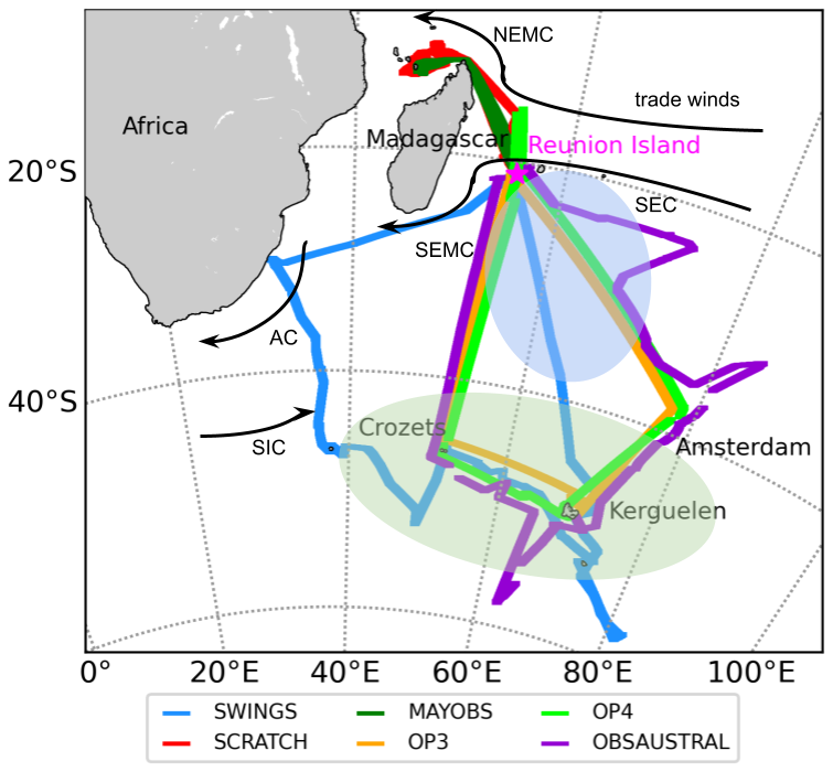
Figure 1 The Marion Dufresne paths covered in 2021 and 2023 during four specific campaigns (SWINGS 2021, SCRATCH 2021, MAYOBS 2021, and OBSAUSTRAL 2023) and two port operations (OP3 and OP4 2021). The paths of OP3, OP4, and OBSAUSTRAL are shifted in longitude (between −1.4 and 1.2°) and latitude (between −1.6 and 1°) from their original location to provide a better view of the different campaigns. The black arrows represent the surface atmospheric and surface oceanic circulation in the region: trade winds, the South Equatorial Current (SEC), the North Equatorial Madagascar Current (NEMC), the South Equatorial Madagascar Current (SEMC), the Agulhas Current (AC), and the South Indian Current (SIC). The green-shaded area is the region where phytoplankton are the most abundant and generally observed in the austral summer. The blue-shaded area is the pristine region observed in the southern Indian Ocean.

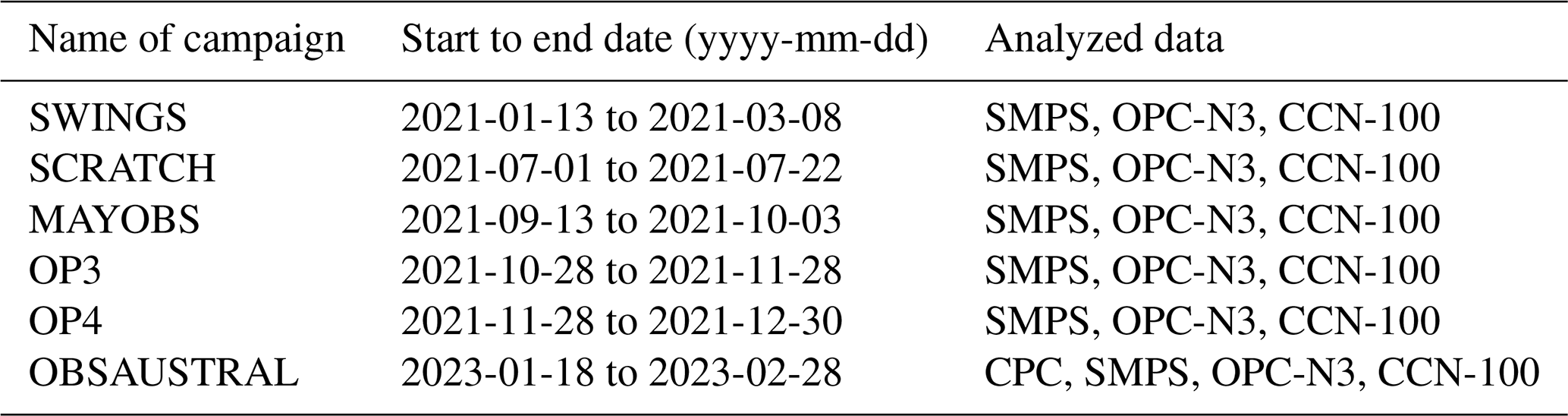
Table 1 Name and duration of the campaigns realized in 2021 and 2023 and list of data analyzed in the present paper.

The SWINGS campaign (Fig. 1; blue track) took place during the austral summer from 13 January to 8 March 2021. The aim was to collect CO₂, pH, and fish population density measurements at different latitudes and depths in the Southern Ocean. During this campaign, the Marion Dufresne route began along coastal regions passing south of Madagascar and southeast of Africa, then moved on to the open ocean, where it stopped at Crozet and then the Kerguelen Islands before returning to Réunion. The SCRATCH campaign (Fig. 1; red track) took place during austral winter and was carried out from 1 to 22 July 2021. The aim was to better characterize the region using a combination of biological and geological techniques. During this campaign, the vessel passed east of Madagascar and stayed in the northern part of the Mozambique Channel before going back to Réunion. The MAYOBS campaign (Fig. 1; green track) was carried out during austral winter from 13 September to 3 October 2021 as part of the monitoring of an underwater volcanic eruption that began around Mayotte in 2018. The route of the vessel was similar to the one during the SCRATCH campaign. The OP3 and OP4 campaigns (Fig. 1; orange and lime tracks) were carried out under the TAAF charter during austral spring from 28 October to 28 November 2021 and from 28 November to 30 December 2021, respectively. During these two campaigns, the Marion Dufresne took the same routes: Réunion–the Crozet Islands–the Kerguelen Islands–Amsterdam Island–Réunion. The OBSAUSTRAL campaign (Fig. 1; purple track) took place during the austral summer in 2023 from 18 January to 28 February. The objectives were the same as those of the SWINGS campaign, including the monitoring of seismic activity at ocean ridges and the identification of cetacean vocal signatures using hydrophones. The vessel's route was similar to the one during OP3 and OP4 with one exception: it went further to the south between the Crozet Islands and the Kerguelen Islands and further to the east between Amsterdam Island and Réunion.

2.2 Geographical and meteorological context

Between 10 and 25° S, westward surface atmospheric and oceanic circulation prevails, characterized by southeast equatorial winds and the South Equatorial Current (SEC) (Fig. 1). In this latitude range, the average wind speed measured on board the Marion Dufresne is 6.7 ± 3.9 m s⁻¹ (Fig. 2a), the average wave height is 2.5 ± 1.2 m (Fig. 2c), and the average nanophytoplankton abundance is 306.1 ± 90.2 cells cm⁻³ (Fig. 2c). Madagascar's high plateaus play a role in regional circulation by splitting the trade winds into two branches: a northeasterly flow, which notably affected the region of the SCRATCH and MAYOBS campaigns, and a southeasterly flow, which affected the beginning of the SWINGS campaign's route between Réunion and Madagascar. The oceanic circulation also divides into two branches at the northeastern tip of Madagascar, with one bypassing the island to the north (North East Madagascar Current, NEMC) and the other to the south (South East Madagascar Current, SEMC) (Fig. 1). Between the southern tip of Madagascar and 30° S, the wind direction progressively changes and becomes eastward when encountering strong westerlies typically extending from 35 to 60° S (Fig. 1). The SEMC flows toward the southeast coast of Africa, where it becomes the Agulhas Current (AC) (Fig. 1). The area extending southeast of Madagascar has been considered pristine in the literature (Fig. 1; blue-shaded area) (Mallet et al., 2018). At 40° S, the AC is retroflected and goes eastward. It then becomes the South Indian Current (SIC) and flows northeastward (Fig. 1). The subantarctic front is located south of it. This current is characterized by a strong sea temperature and salinity gradient between the subtropical zone and the Antarctic zone, which marks the northern boundary of the Southern Ocean (Giglio and Johnson, 2016). The Marion Dufresne crossed the subantarctic front during the SWINGS, OBSAUSTRAL, OP3, and OP4 campaigns. In this area, phytoplankton blooms – driven by nitrate, phosphate, or iron water fertilization – were observed during the austral summer on the Crozet Islands (46° S, 51° E) and Kerguelen Plateau (49, 69° S) (Sedwick et al., 2002; Blain et al., 2008). Measurements of nanophytoplankton abundance were performed during SWINGS and OBSAUSTRAL, during the austral summer, and showed a clear signal of enhancement between 40–55° S (Fig. 2c). The polar front is further south between 55 and 60° S and marks the boundary between the warmer subantarctic water and the cold Antarctic water. The Southern Ocean is the roughest ocean on Earth due to the absence of land (Young, 1999). Even in the austral summer, Derkani et al. (2021) measured average wind speeds of 11 m s⁻¹ and swells in excess of 3.5 m. During the SWINGS and OBSAUSTRAL campaigns, average winds also exceeded 10 m s⁻¹, and average wave heights exceeded 5 m. Three major storms were documented during the SWINGS campaign in 2021 (Fig. 1a; black circles). The first one was located south of the Crozet Islands, the second one south of the Kerguelen Islands, and the third one north of the Kerguelen Islands. The maximum wind speed was 23, 33, and 27 m s⁻¹, respectively. The predominant wind direction was from the northwest south of the Crozet Islands and the Kerguelen Islands and from the southwest north of the Kerguelen Islands (Fig. 2b). The maximum wave height was 14, 21, and 15 m, respectively (Fig. 2c). The nanophytoplankton abundance was lower (400–800 cells cm⁻³) along the storm tracks (Fig. 2d) due to a more intense mixing that deepened the ocean mixing layer and limited the light available for phytoplankton growth (Fragoso et al., 2024). It is important to note that the local wind direction observed during the campaigns is highly variable and differs from the general wind circulation presented in Fig. 1. Therefore, in order to conduct a thorough analysis of particular periods within the campaigns, it is imperative to pay close attention to the local measurements of wind. For more information on the climatology of the southwestern Indian Ocean and the Southern Ocean, see for example the studies by Schott et al. (2009) and Mondal et al. (2022).

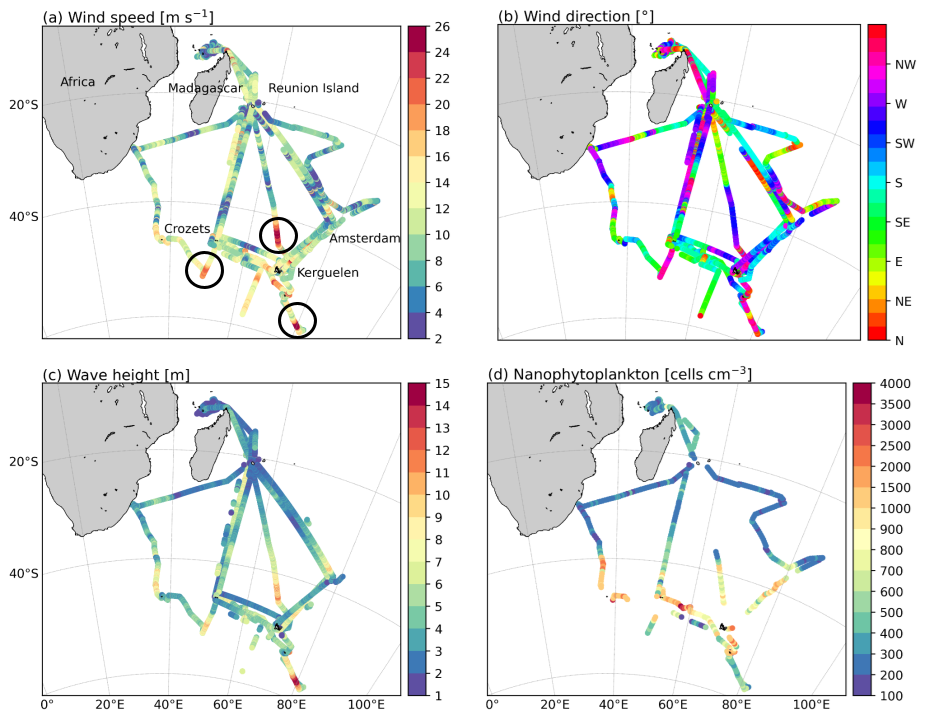
Figure 2 Marion Dufresne path colored according to (a) wind speed, (b) wind direction, (c) wave height, and (d) nanophytoplankton abundance during the six campaigns analyzed. The three storms that occurred during SWINGS are circled in black.

2.3 Instrumentation

In the framework of the MAP-IO program, the Marion Dufresne has been equipped with 19 measurement and remote sensing instruments, described in Tulet et al. (2024). Among the 19 instruments, 7 are dedicated to the study of aerosols and atmospheric gas. In Fig. 3, the top-left and top-right pictures present the aerosol and gas inlets located at the center of the vessel, upstream of the exhaust stack and 21 m above the sea level. The bottom picture of Fig. 3 shows the aerosol and gas acquisition system and analyzers located in the meteorological laboratory and mounted on a shock-absorbing table.

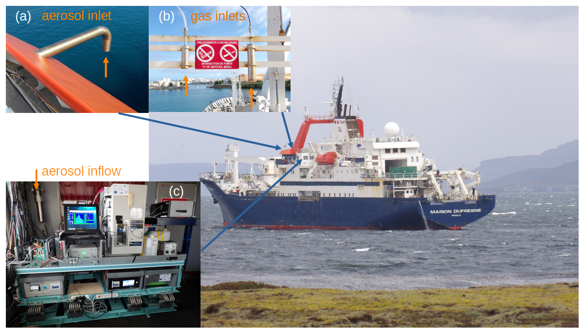
Figure 3 Picture of the Marion Dufresne in the Port-aux-Français bay (February 2024). (a) The aerosol and (b) gas inlets are located above the wheelhouse. (c) The acquisition and monitoring system is located in the meteorological room next to the wheelhouse and mounted above a shock-absorbing table. Aerosol monitoring systems are on the top shelf, to the right of the acquisition computer. Gas analyzers are on the bottom shelf. Photography credits: Meredith Dournaux.

Aerosol inflow enters the same sampling line, which, after passing through a Nafion tube used to dry the aerosol, divides and directs the flow toward the different instruments. The distance between the inlets and the instruments (8 m) was carefully chosen to minimize aerosol losses along the sampling line. To minimize the loss of the largest particles (> 1 µm), three OPC-N3 sensors are installed directly outside on the main deck. A water-based condensation particle counter (CPC; MAGICTM-200/210) measures the particle number concentration within the size range of 5 nm to 2.5 µm using a condensational growth system. A scanning mobility particle sizer (SMPS; 4S) is used to measure the number size distribution of aerosols. It is composed of a differential mobility particle sizer (DMPS) and a CPC (MAGICTM-200/210). The DMPS takes in the aerosol flow composed of dry particles and cloud droplets, and the water of the latter is evaporated while penetrating the inlet. The aerosol population is first neutralized using an X-ray neutralizer (TSI) to provide the same electrical charge to all particles, then selected using their size-dependent electrical mobility and classified into 133 bins from 3 to 350 nm. The number of aerosols per bin is then determined by the CPC. The whole size range is scanned in 5 min.

To complete the aerosol size distribution toward supermicron diameters, three optical particle counters (OPC-N3, Alphasense) are used to measure the number concentration and the size of particles within the size range of 0.35 to 40 µm. Using a calibration based on Mie theory, the OPC-N3 measures the light scattered by each particle of a sample airflow (sample flow rate of 210 mL min⁻¹) passing through a 658 nm laser beam. The particle size and concentration are determined according to the intensity of the scattered light and allow the classification of each particle into one of the 24 bins covering the measurement size range at a rate of about 10 000 particles s⁻¹. Generally, 100 % of the particles are detected at 0.35 µm and 50 % at 40 µm (Alphasense user manual, http://www.alphasense.com, last access: 1 September 2025). In our case, as the OPC-N3 sensors have no sampling line and are directly located outside, there is no loss of large aerosols, except on the walls of the instruments. To study the aerosol activation properties, a cloud condensation nuclei counter (CCN-100, DMT) is used to measure the number concentration of activated aerosols at different supersaturation levels (SS of 0.1 %, 0.2 %, 0.3 %, 0.4 %, 0.5 %, 0.6 %, 0.8 %, and 1.0 %), with the first two set for 15 min and the others for 5 min. Supersaturation is created by three temperature control zone columns mounted vertically. The aerosol sample enters at the top of the column and becomes progressively supersaturated with water vapor as it goes through the column. Activated droplets are then counted by an internal OPC and distributed into 20 size bins going from 0.75 to 10 µm. Gas measurements are realized by an NO_x analyzer (Teledyne N500 CAPS), an O₃ analyzer (HORIBA APOA-370), and a Picarro analyzer (Picarro G2401 CFKADS-2372) measuring atmospheric gas traces as CO, CO₂, CH₄, and H₂O (ppb). The gas inlets are located to the right of the aerosol inlet (Fig. 3b). Along with aerosol measurements, wind speed (m s⁻¹), and wind direction (°), air temperature (°C), pressure (hPa), and humidity (%) are recorded by the Vaisala and Mercury meteorological stations with a sampling time step of 5 s and 1 min, respectively. Sea surface elevation (m) and ship position are also recorded by the inertial unit of the ship at a sampling time step of 1 s.

3 Data processing

3.1 Data filtering

First, the data are filtered to remove all the measurements likely to be contaminated by the exhaust of the vessel. Observations of time series of the total number concentration and the relative wind direction concluded that measurements realized within the direction range of 90–225° were associated with high aerosol concentrations (> 5000 cm⁻³) lasting over time. A second filter – combining relatively low wind speed, vessel cruise speed, and gas concentration data – was applied in an attempt to remove local episodes of pollution. Thus, all data collected at wind speeds below 2 m s⁻¹, which may have inhibited pollution plume dilution around the inlets, were removed. In addition, data were removed when the ship was stationary, thus eliminating contamination by maintenance activities on board (painting, rust removal). To complete the filter, data with corresponding high concentrations of NO and NO₂ (> 1 ppbv) were removed, with the latter being relatively low (< 1 ppbv) in remote marine environments. CO peaks in concentration were also identified following the semi-automatic method of detection described in El Yazidi et al. (2018). The use of different chemical tracers was not only useful when one of the analyzers did not work properly, but also useful for confirming the good agreement between NO_x and CO concentrations. A third step consisted of the quality control of the aerosol data. For SMPS data, the particle size distributions were filtered manually for each measurement to remove non-physical variations (e.g., local pollution undetected by the dynamic and chemical filters). The latter were noticeable by an abrupt and short increase in the concentration of aerosols over the entire range of diameters, known as “spikes”. SMPS data were quality controlled and corrected over the sampling periods using CPC data.

The original raw SMPS dataset consisted of 55 144 measurements of aerosols, which represent ∼ 192 d of measurements. After the first and second filtering steps, it consisted of 53 201 measurements. After the manual filtering step, 36 226 measurements were conserved, which represent ∼ 66 % of the original dataset. In total, 29 376 measurements were taken in 2021 and 6850 measurements in 2023, as shown in Fig. 1. The start and end dates of each campaign are shown in Table 1. The data collected in 2022 were not used in this study due to SMPS maintenance and calibration.

3.2 Activation diameter and hygroscopicity parameter

First, the CCN-100 data at 0.2 % and 0.4 % supersaturation were treated separately, and only the data recorded on the plateau (measurements realized approximately 3 min after a supersaturation change according to our experience) were averaged over 5 min to make them comparable to SMPS data. Assuming that aerosols are internally mixed and that larger particles are activated preferentially before the smallest ones due to the curvature effect, we can determine the hygroscopicity of aerosols at the activation diameter by calculating activation diameters and deriving the hygroscopicity parameter at both supersaturation levels. Activation diameters were then calculated using the total number of cloud condensation nuclei given by the CCN-100 and the number concentration of aerosols measured in each bin by the SMPS. The number of aerosols per bin was integrated from the largest diameter to the smallest until it matched the number of CCN. The activation diameter corresponds to the smallest diameter. The hygroscopicity parameter, kappa–Köhler, was derived from the previously determined activation diameters as follows (Petters and Kreidenweis, 2007):

$$\begin{array}{}\text{(1)}& {\displaystyle }\mathit{\kappa }={\displaystyle \frac{\mathrm{4}{A}^{\mathrm{3}}}{\mathrm{27}{D}_{\mathrm{d}}^{\mathrm{3}}{\ln }^{\mathrm{2}}{S}_{\mathrm{c}}}},\text{(2)}& {\displaystyle }A={\displaystyle \frac{\mathrm{4}{\mathit{\sigma }}_{s/a}{M}_{\mathrm{w}}}{RT{\mathit{\rho }}_{\mathrm{w}}}},\end{array}$$

where A is composed of ${\mathit{\sigma }}_s/a$ = 0.072 J m⁻², the surface tension of pure water; M_w = 0.018 kg mol⁻¹ is the molecular weight of water; R = 8.314 $\mathrm{J}{\mathrm{mol}}^{-\mathrm{1}}{\mathrm{K}}^{-\mathrm{1}}$ is the perfect gas constant; T is the activation temperature in K; and ρ_w = 997 kg m⁻³ is the density of water. D_d is the activation diameter in nm calculated for a given supersaturation S_c. Note that hygroscopic particles have theoretical kappa values between 0.5 and 1.4. Petters and Kreidenweis (2007) summarized several κ values derived from CCN measurements. κ values are 1.28 and 0.9 for NaCl and H₂SO₄, respectively. When the Na⁺ ion is associated with other compounds, its κ values decrease and range between 0.8 and 0.88. Ammonium sulfate has κ values between 0.61 and 0.67. Organic compounds have κ values between 0.01 and 0.4, and hydrophobic aerosols, such as black carbon, have values of 0.

3.3 Air mass classification

Back trajectories provide additional information to understand the origin of the air mass and thus help to better understand the observed aerosol size distribution and properties. For this purpose, the FLEXible PARTicle (FLEXPART) version 10.4 model (Pisso et al., 2019) was used from the vessel's position.

The FLEXPART model is part of the multi-scale offline Lagrangian particle dispersion models (LPDMs), which have been developed to simulate transport and turbulent mixing of aerosols and gases in the atmosphere. The model can be run for forward or backward simulations. In backward mode, the location where particles are released, called a “receptor”, is defined within a longitude–latitude–altitude cell (Pisso et al., 2019). For this study, ERA5 meteorological fields with a spatial resolution of 0.5° × 0.5° and time resolution of 1 h were used as input, and 5 d back trajectories were run each hour of the campaign at the location of the vessel with a particle release between 0 and 50 m altitude. To analyze the dataset according to the air mass origin, the area covered by the vessel was divided into three subdomains related to the main types of air masses. Continental air masses were identified as such when their residence time over the area north of 40° S and west of 50° E was the greatest. Air masses were classified into the subtropical Indian Ocean group when their residence time over the area east of 50° E and north of 40° S was the greatest. Thus, southern Indian Ocean air masses were identified as such when their residence time over the area south of 40° S was the greatest. This classification led to 15 385 receptors in the southern Indian Ocean group (with a spatial extension of 20–60° S and 35–80° E), 5495 receptors in the subtropical Indian Ocean group (with a spatial extension of 20–50° S and 55–80° E), and 4048 receptors in the continental group (mostly located north of Madagascar and around Réunion). This classification also resulted in a mixed zone where all three types of air mass are present in the middle of the subtropical Indian Ocean. This classification resulted in 6273, 18 647, and 9049 SMPS data points (0.02–0.35 µm) and 2305, 13 727, and 5554 OPC-N3 data points (0.41–5.85 µm) used in the calculation of the average aerosol size distribution of the continental, southern Indian Ocean, and subtropical Indian Ocean air masses, respectively.

4 Spatial and temporal variability in marine aerosol properties

Aerosol number concentration (N_SMPS) was calculated by summing the SMPS diameters ranging from 3 to 350 nm. Figure 4 shows the spatial variation in N_SMPS (Fig. 4a), the cloud condensation nuclei concentration at 0.4 % SS (N_CCN) (Fig. 4b), the activation diameter (D_act) at 0.4 % SS (Fig. 4c), and the kappa–Köhler parameter (κ) at 0.4 % SS (Fig. 4d) along the vessel track during the six campaigns.

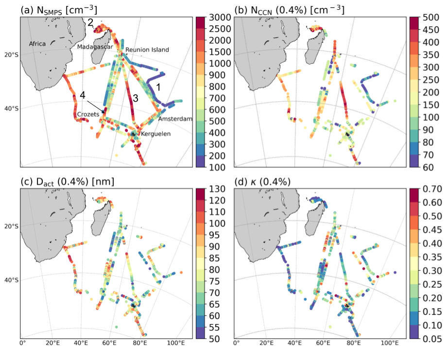
Figure 4 (a) Evolution of N_SMPS measured by the SMPS from 3 to 350 nm, (b) N_CCN at 0.4 % SS, (c) D_act at 0.4 % SS, and (d) κ at 0.4 % SS along the path of the Marion Dufresne in 2021 and 2023.

N_SMPS is highly variable in the sampling area, with a difference of 1 order of magnitude between low and high concentrations. The average N_SMPS is 1149 ± 706 cm⁻³ (mean ± 1 standard deviation), with ∼ 95 % of the values between 100 and 3000 cm⁻³. The average N_CCN at 0.4 % SS is 208 ± 102 cm⁻³, with ∼ 95 % of the values between 60 and 500 cm⁻³. To further investigate the hygroscopic properties of the aerosol population, the spatial variations in the activation diameter and κ were calculated according to Petters and Kreidenweis (2007) (Sect. 3.2). Activation diameters are highly variable (between 50–130 nm) along the different routes taken by the Marion Dufresne, with an average value of 80 ± 15 nm (Fig. 4c). Moreover, 98 % of the κ values are in the physical range between 0.05–0.7 at 0.4 % SS, with an average value of 0.2 ± 0.1 (Fig. 4d). This indicates a large variability in the chemical composition and size distribution of aerosols in the southern Indian Ocean and the Southern Ocean.

The difference in the location of high and low aerosol concentrations reflects different underlying processes. N_SMPS less than 200 cm⁻³ (Fig. 4a; label 1) is mostly observed in the eastern part of the Indian Ocean (20–40° S, 60–80° E) during OBSAUSTRAL. In this region, 90 % of N_SMPS is less than 300 cm⁻³ and shows low variability. These low concentrations are explained by the observed weak to moderate wind speed (< 10 m s⁻¹) (Fig. 2a) and by the area being far from any continent. Similarly, N_CCN is generally less than 70 cm⁻³, which corresponds to the lowest concentrations observed across all campaigns (Fig. 4b).

N_SMPS greater than 1000 cm⁻³ is mostly observed north of Madagascar (Fig. 4a; label 2). In this area (0–20° S, 40–50° E), only 7 % of the data have N_SMPS below 500 cm⁻³. High concentrations of CO, CO₂, CH₄, and O₃ were also observed (Tulet et al., 2024), suggesting a continental influence in these areas. This region is also associated with an average N_CCN of 271 ± 86 cm⁻³. The activation diameters are generally greater than 80 nm (Fig. 4c), and the associated κ drops to values between 0.05 and 0.15, corresponding to aerosols that are mostly hydrophobic.

A high N_SMPS value, between 900 and 3000 cm⁻³, is also observed along the transects where the Marion Dufresne encountered storms during SWINGS (Fig. 2a; black circles). However, as is clearly visible along the transect between the Kerguelen Islands and Réunion, this high N_SMPS concentration is not limited to the wind speed peaks (south of 40° S) and extends further north (Fig. 4a; label 3). Along this transect, N_CCN varies similarly to N_SMPS, with concentrations between 250 and 500 cm⁻³. The activation diameter increases from 50 to 120 nm as the vessel approaches Réunion. The κ values are first between 0.2 and 0.5 in the maximum wind speed region, then gradually decrease from 0.6 to 0.2 between 40° S and Réunion (Fig. 4d).

Another period is marked by a sharp increase in N_SMPS from 400 to more than 3000 cm⁻³ between 35° S and the Crozet Islands during OP3 (Fig. 4a; label 4). However, along this transect, N_CCN (200–350 cm⁻³) does not follow the increase in N_SMPS and changes little. It is also observed that the activation diameter (70–90 nm) and κ (0.1–0.2) vary little, suggesting that the increase in N_SMPS comes from particles smaller than the activation diameter.

To explain this variation in N_SMPS in the region, the four situations presented in the present section are discussed below.

5 Case studies

Among the numerous situations observed during the six campaigns presented in this paper, several deserve to be detailed in order to analyze their origins or specific processes. Four types of situations (Fig. 5) have been selected, which led to N_SMPS observations smaller than 200 cm⁻³ or peaks above 3000 cm⁻³.

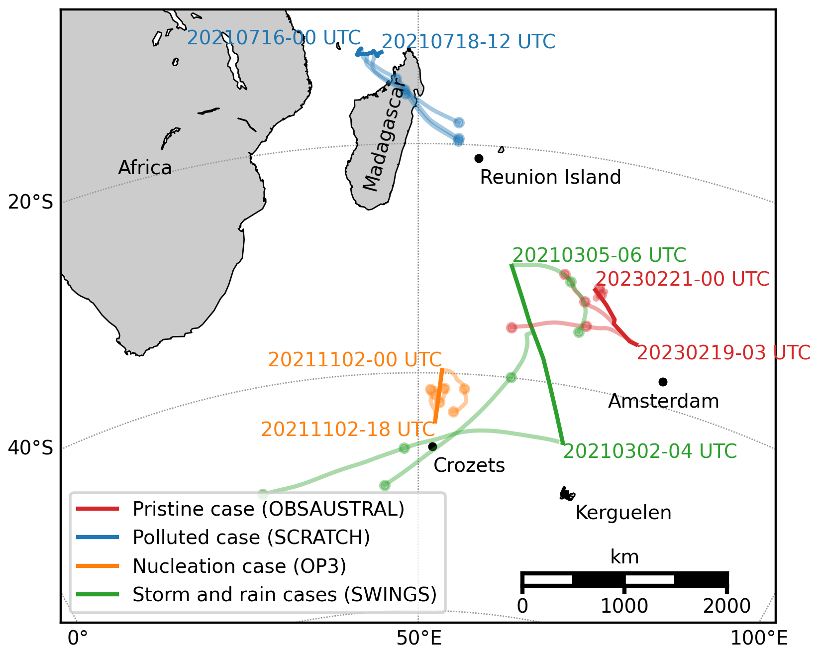
Figure 5 Position of the Marion Dufresne (thick lines) and 2 d back trajectories (thin lines) from the FLEXPART model for the four selected situations, illustrating the origins of the air masses (one dot per day).

5.1 Pristine case (OBSAUSTRAL)

A case of pristine air mass observed on 19 and 20 February 2023 is shown in Fig. 6 and is associated with the low N_SMPS observed along the easternmost transect of OBSAUSTRAL (Fig. 4a; label 1). During this period, the air masses arriving at the ship's position evolved over the subtropical Indian Ocean, far from the continents. The height of the back trajectory shows that the air mass remained in the oceanic boundary layer, i.e., below 1000 m, for the 3 d prior to the measurement (Fig. 6a to d). During this period, the aerosol size distribution is very stable, with a clearly visible Aitken mode around 50 nm and a weak and broad accumulation mode between 150 and 300 nm. This large accumulation mode mean diameter and the lack of mode evolution indicate that the air mass is aged (Fig. 6e). N_SMPS and N_CCN remained low, between 150–250 and 40–120 cm⁻³, respectively (Fig. 6f). Throughout the day, the activation diameter is between 60 and 140 nm and lies between the Aitken mode and the accumulation mode in a very low concentration zone close to the measurement noise. The κ values obtained range from 0.1 to 0.5 at 0.2 % SS and from 0.1 to 0.3 at 0.4 % SS. Specifically, when N_SMPS and N_CCN concentrations are exceptionally low, it has been observed to induce a decrease in κ. This decrease occurs without any discernible pattern in the particle size distribution or in the origin of the air mass. This situation illustrates a case where the calculation of κ based on the combination of two instruments exhibits an important sensitivity to low concentrations. Consequently, the resultant value should be considered with caution.

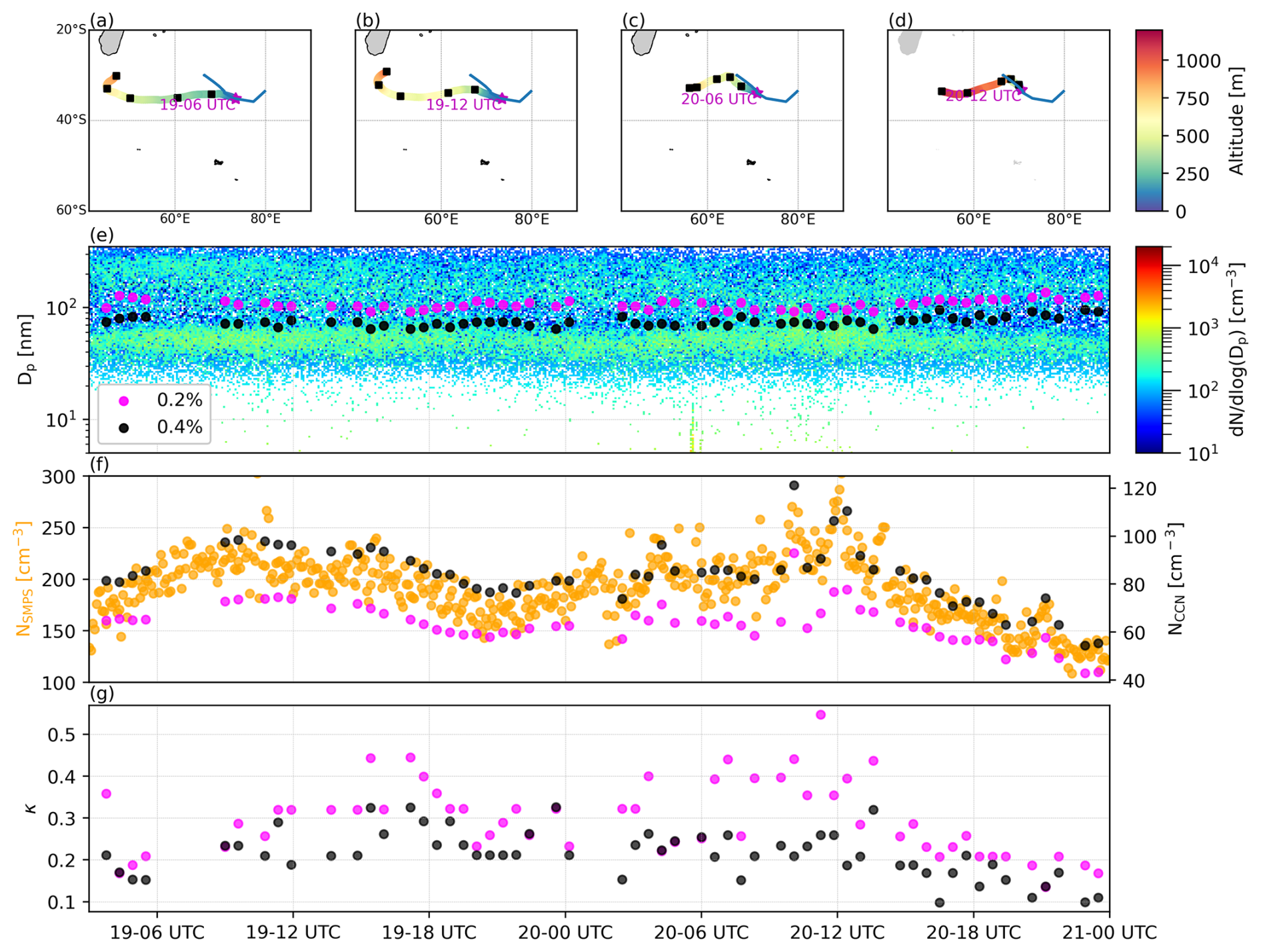
Figure 6 (a–d) The 10 m wind speed from ERA5 along four FLEXPART back trajectories at four instances. The blue contours correspond to areas where the rain rate is higher than 0.1 mm h⁻¹ at that instant. (e) Temporal evolution of aerosol size distribution and activation diameter, (f) aerosol concentration (N_SMPS) and cloud condensation nuclei (N_CCN) at 0.2 % and 0.4 % supersaturation, and (g) hygroscopicity parameter (κ) at 0.2 % and 0.4 % supersaturation observed on 19 and 20 February 2023 during the OBSAUSTRAL campaign (Fig. 1).

5.2 Polluted case (SCRATCH)

Figure 7 shows the evolution of the aerosol particle size distribution (Fig. 7e), N_SMPS concentrations (Fig. 7f), and CO concentrations (Fig. 7h) between 16 and 19 July 2021. The origin of the air mass is also represented by the height of the back trajectory over the period (Fig. 7a to d). During this period, CO and N_SMPS concentrations remained high (> 50 ppb and > 2000 cm⁻³, respectively), showing that the area was generally affected by residual continental pollution. The activation diameter remained high (∼ 128 nm at 0.2 % SS and ∼ 92 nm at 0.4 % SS), and κ values were less than 0.19. Several peaks of N_SMPS > 6000 cm⁻³ were also measured periodically and are associated with a significant increase in CO concentrations of 10 to 15 ppb, indicating that the air mass was affected by anthropogenic pollution. The aerosol size distribution shows that these N_SMPS peaks are associated with an increase in the number of aerosols in the Aitken mode (30 to 40 nm) and the appearance of a new nanoparticle mode located between 5 and 30 nm. The back-trajectory analysis clearly shows the passage of the air mass at about 800 m a.g.l. over the urbanized region of Majunga, northwest Madagascar. The temporal evolution of the mixing boundary layer (MBL) thickness over Madagascar, corrected for transport time, is shown in Fig. 7h. There is a clear correlation between the MBL thickness and the CO and N_SMPS peaks: each concentration peak is associated with an MBL thickness greater than 800 m. This means that only the upper part of the polluted boundary layer over Madagascar can reach the ship by subsidence. This can only happen in the afternoon when the boundary layer is sufficiently developed. This situation shows that the high variability in aerosol concentration between 800 and 8000 cm⁻³ observed in the northern Mozambique Channel (Fig. 4a; label 2) can be explained by a residual polluted air mass that evolves with the diurnal evolution of the MBL over Madagascar. This important aerosol number has a small impact on N_CCN. Moderate N_CCN observed range from 100 to 500 cm⁻³ and are attributed to elevated activation diameter values (> 100 nm) that exceed the residual continental pollution mode. The resulting κ is low, ranging from 0.06 to 0.1 at 0.4 % SS and from 0.1 to 0.2 at 0.2 % SS. This indicates an air mass composed primarily of hydrophobic aerosols.

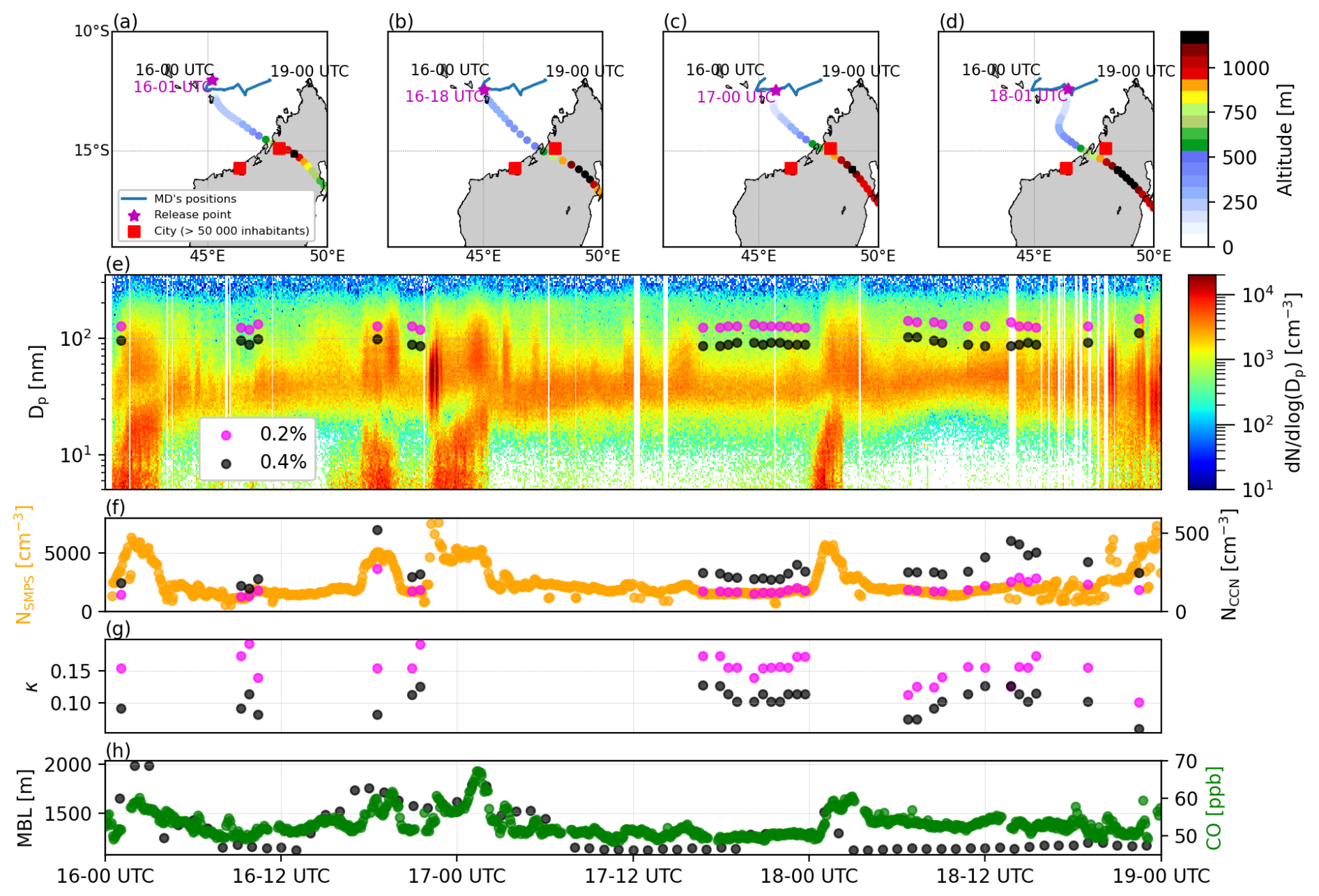
Figure 7 (a) 16 July, 00:00 UTC; (b) 16 July, 18:00 UTC; (c) 17 July, 00:00 UTC; (d) 18 July, 01:00 UTC. (e) Temporal evolution of aerosol size distribution and activation diameter and (f) aerosol number concentration (N_SMPS) and cloud condensation nuclei concentration (N_CCN) observed from 16 to 19 July 2021 (SCRATCH campaign, Fig. 1). (g) Aerosol hygroscopicity (κ) at 0.2 % SS and 0.4 % SS. (h) CO concentration at the Marion Dufresne location and mixing boundary layer (MBL) thickness evolution during the first 3 h over western Madagascar along FLEXPART back trajectories. Altitude of air masses along FLEXPART back trajectories for the four CO peaks. The red squares correspond to the locations of the most urbanized areas in Majunga Province (Madagascar).

5.3 Storm and rain case (SWINGS)

The third period highlighted corresponds to a case of primary aerosol emission observed during the SWINGS campaign between 2 March 2021 at 00:00 UTC and 6 March 2021 at 00:00 UTC. Three periods can be identified. On 2 March, prior to 06:00 UTC, the air mass moved from the west into a storm zone and was characterized by ERA5 winds that exceeded 18 m s⁻¹ (Fig. 8a). The vessel was affected by this storm, with measured swells exceeding 14 m and wind speeds reaching 25 m s⁻¹. The air mass was also under the influence of rain, which limited the aerosol concentration due to washout, particularly prior to 03:00 UTC (∼ 500 cm⁻³) (Fig. 8a, d, e). The activation diameter was observed to range between 60 and 100 nm, with significant fluctuations in hygroscopicity, as indicated by variations in κ, ranging from 0.2 to 1 (Fig. 8f). During the second period, from 2 March at 18:00 UTC to 3 March at 06:00 UTC, a decline in wind and wave height conditions was recorded (Fig. 8b, g). On 2 March at 18:00 UTC, the ship moved approximately 300 km northwestward. The measured wind and wave height remained elevated, and the air mass continued to be exposed to strong winds exceeding 20 m s⁻¹ over the past 24 h. According to the ERA5 analyses, this air mass was not affected by rain. This explains why the aerosol concentrations measured on the Marion Dufresne exceeded 3000 cm⁻³ despite the slight decrease in wave height and wind intensity. Aerosol hygroscopicity increased overall but remained variable, with kappa ranging from 0.2 to 1 (Fig. 8f). The third period begins at 06:00 UTC on 3 March. SMPS data show the persistence of a pronounced Aitken mode of around 30 nm and a concentration of approximately 2000 cm⁻³ (Fig. 8d, e). The formation of a second mode is also observed, whose size increases over the period and reaches a size characteristic of the accumulation mode of around 100 nm. During this period, the Marion Dufresne maintained a northwestward course, away from the storm center. According to the ERA5 data, on 3 March at 18:00 UTC, the air mass remained unimpacted by rain and had experienced moderate winds of approximately 10 m s⁻¹ the previous day (Fig. 8c). Observations from the Marion Dufresne indicate that the sea remained rough until at least 06:00 UTC on 4 March, with wave heights ranging between 6 and 10 m (Fig. 8g). Although the total aerosol concentration remained largely stable during this period, it is noteworthy that as the air mass aged, an accumulation mode emerged (probably through coagulation processes), resulting in a continuous decline in κ from 0.7 on 3 March at 06:00 UTC to 0.2 on 5 March at 00:00 UTC (Fig. 8f). As a partial conclusion, the findings indicate that the aerosol concentration is determined by the equilibrium between various factors, including advection, local primary production, and loss through precipitation. It is important to note that the maximum concentration of aerosols is not necessarily attained during periods of peak wind speed and wave height.

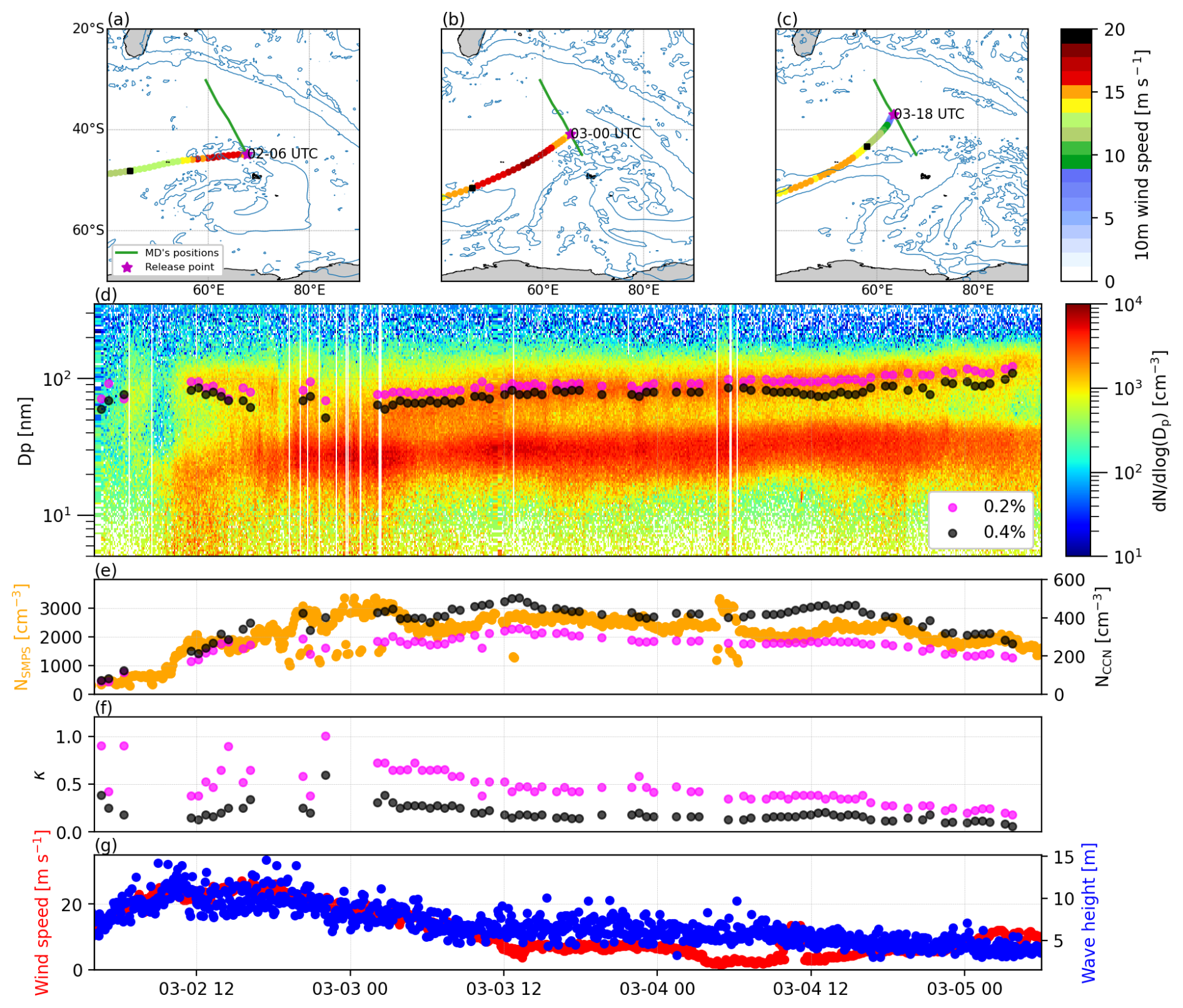
Figure 8 (a–c) The 10 m wind speed from ERA5 along three FLEXPART back trajectories at three instances. The blue contours correspond to areas where the rain rate is higher than 0.1 mm h⁻¹ at that instant. (d) Temporal evolution of aerosol size distribution and activation diameter and (e) aerosol concentration and cloud condensation nuclei at 0.2 % SS and 0.4 % SS. (f) Hygroscopicity parameters at 0.2 % SS and 0.4 % SS. (g) Wind speed and wave height observed from 2 to 5 March 2021 during the SWINGS campaign (Fig. 1).

5.4 Nucleation case (OP3)

Figure 9 shows the evolution of the aerosol concentration (N_SMPS, N_CCN, and size distribution) and ship tracks superimposed on a cloud mask based on satellite brightness temperature (cloud areas correspond to brightness temperatures below 282 K; e.g., Janowiak et al., 2017; Wang et al., 2017) on 11 September 2021. The satellite images in Fig. 9a–d show that the ship was in a cloudy area until 07:00 UTC (11:00 LT), then passed through a clear-sky area between 09:00 and 15:00 UTC, before returning to a cloudy area. Before 08:00 UTC (∼ 12:00 LT), SMPS measurements clearly show two modes at 30 and 130 nm, associated with an N_SMPS of 500 cm⁻³. The measured N_CCN is low: 178 cm⁻³ at 0.2 % SS and 221 cm⁻³ at 0.4 % SS. κ is between 0.1 and 0.4. A sharp increase in N_SMPS is observed at 09:00 UTC, reaching 4000 cm⁻³ at 13:00 UTC. The SMPS size distribution depicts the formation of new particles at 09:00 UTC (5 nm), which is associated with classic banana-shaped growth (condensation–coagulation) that is characteristic of nucleation events (Kulmala and Kerminen, 2008; Foucart et al., 2018; Määttänen et al., 2018, and references cited). In addition, the formation of new particles is concomitant with the transition from cloudy to clear skies. The activation diameters at 0.2 % SS and 0.4 % SS are larger than the size of the nucleation mode. During the nucleation process, the Aitken mode demonstrates growth from 30 to 80 nm, which exceeds the activation diameter at 0.4 % SS. Thus, the N_CCN at 0.4 % SS increases from 220 cm⁻³ (08:00 UTC) to 350 cm⁻³ (10:00 UTC), while the N_CCN at 0.2 % SS remains relatively stable throughout the day. κ at 0.2 % of SS increases at 0.46. This increase in hygroscopicity is likely associated with the condensation of semivolatile oxidized species on the Aitken mode, which undergoes a simultaneous evolution from a median diameter of 50 to 90 nm. This nucleation situation observed during OP3 (Fig. 4a; label 4) demonstrates the possibility of a rapid increase in the number of marine aerosols in pristine areas without being associated with strong increases in CCN concentration.

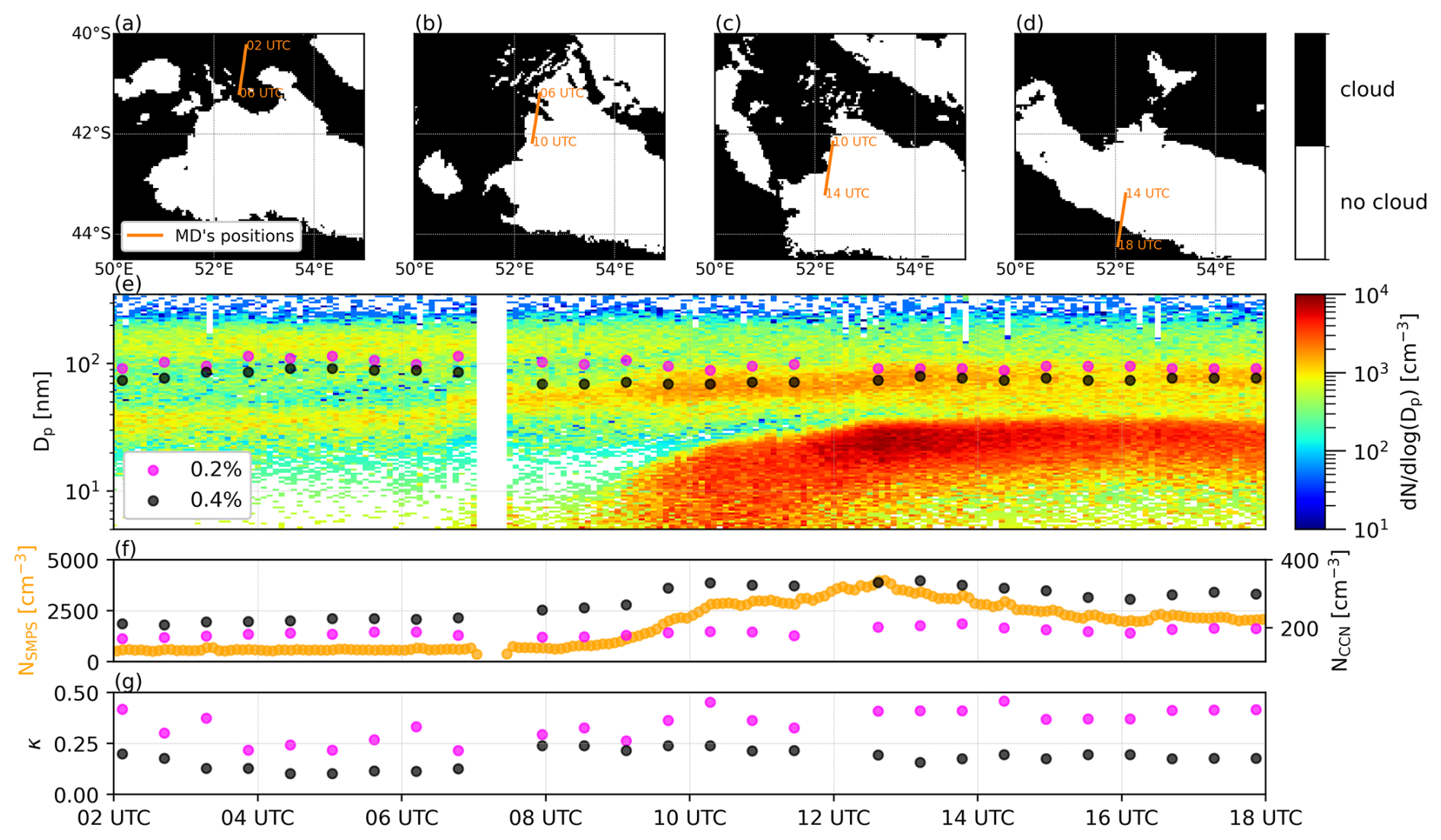
Figure 9 (a) 02:00–06:00 UTC, (b) 06:00–10:00 UTC, (c) 10:00–14:00 UTC, and (d) 14:00–18:00 UTC. Cloud cover and the Marion Dufresne positions. (e) Temporal evolution of aerosol size distribution and activation diameter at 0.2 % SS and 0.4 % SS. (f) Aerosol concentration and cloud condensation nuclei at 0.2 % SS and 0.4 % SS. (g) Hygroscopicity at 0.2 % SS and 0.4 % SS observed on 2 November 2021 (OP3 campaign, Fig. 1).

6 Aerosol size distribution based on its air mass origin

6.1 Size distribution of marine aerosol particles

Figure 10 shows the average aerosol size distributions as a function of air mass origin calculated by FLEXPART using the method described in Sect. 3.3. Table 2 presents the corresponding geometric parameters for each mode fitted to a log-normal distribution.

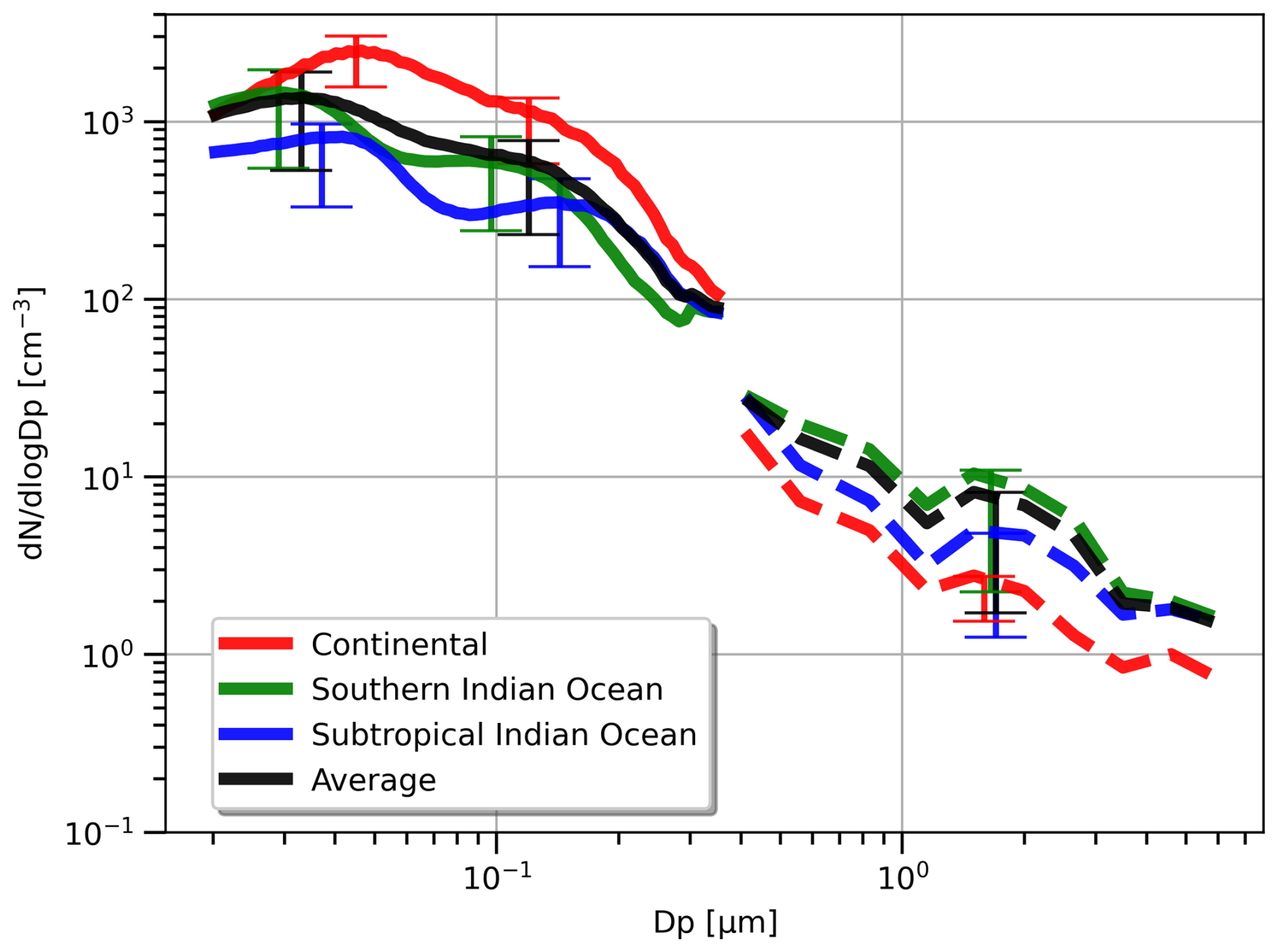
Figure 10 Average size distributions of aerosols according to the air mass origin (continental, southern Indian Ocean, or subtropical Indian Ocean) of the 5 d back trajectories simulated by the FLEXPART model. The solid lines are average size distributions derived from SMPS data, and the dashed lines are average size distributions derived from OPC-N3 data. The bottom and top limits of the error bars, centered in the mean geometric diameter of each mode, are the 25th and 75th quartiles.

Table 2 Geometric parameters of each mode of aerosol's average size distributions (mean diameter, log-normal standard deviation, and total number concentration).

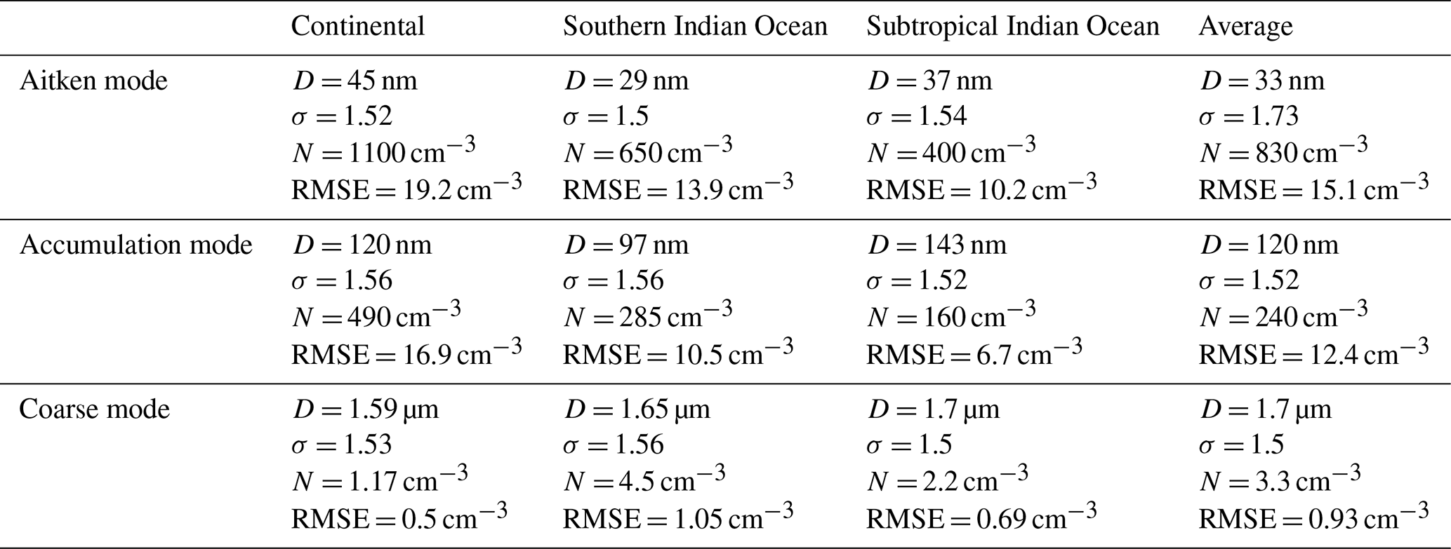
Regardless of the origin of the air mass, we can highlight the Aitken, accumulation, and coarse modes. The mean diameters of the Aitken, accumulation, and coarse modes are 33, 120, and 1.7 µm, and the standard deviations are 1.73, 1.52, and 1.5, respectively.

For the coarse mode, the mean aerosol number concentration is the highest for air masses originating in the southern Indian Ocean (4.5 cm⁻³) and the lowest for continental air masses (1.17 cm⁻³). These concentrations correspond to the presence of strong regular winds and swells in the southern Indian Ocean that generate significant primary emissions.

Significant differences are observed in the submicron modes between different types of air masses. The average aerosol number concentration is 830 cm⁻³ for the Aitken mode and 240 cm⁻³ for the accumulation mode. Continental air masses have concentrations of 1100 cm⁻³ for the Aitken mode and 490 cm⁻³ for the accumulation mode. Similarly, the cleaner air masses from the subtropical Indian Ocean exhibit the lowest average concentrations, with 400 and 160 cm⁻³ for the Aitken and accumulation modes, respectively. Significant differences are also observed for the mean diameter. Air masses from the southern Indian Ocean, which are more influenced by primary emissions, have the smallest diameters: 29 nm for the Aitken mode and 97 nm for the accumulation mode. Larger mean diameters are observed in the continental and subtropical groups of the Indian Ocean. For the Aitken mode, the mean diameter is 45 and 37 nm. For the accumulation mode, the mean diameter is 120 and 143 nm. The Aitken mode of the continental group has the largest average diameter, and there is no clear separation in terms of number concentration between this mode and the accumulation mode. This distinction is particularly noticeable when compared to air masses from the subtropical Indian Ocean group. This can be explained by the pollutant load (gases and aerosols) of the continental group, which favors growth through condensation and coagulation. In contrast, air masses from the subtropical Indian Ocean group are generally cleaner and therefore have less opportunity to grow.

6.2 Relationship between marine aerosol hygroscopicity, wind speed, and nanophytoplankton abundance

Figure 11a, b, and c show the evolution of κ values at 0.2 % SS and 0.4 % SS and Δκ as a function of local wind speed, local nanophytoplankton abundance, and the three types of air masses. The difference in κ indicates the evolution of small-particle hygroscopicity between the two activation diameters (∼ 100 nm at 0.2 % SS and ∼ 80 nm at 0.4 % SS). Nanophytoplankton abundance values are higher for the southern Indian Ocean group, with a mean value of 884.8 ± 166.9 cells cm⁻³ compared to a mean value of 267.4 ± 29.6 cells cm⁻³ for the subtropical Indian Ocean group. The separation between the three types of air masses is clearly visible. The highest average κ values are observed for air masses from the subtropical Indian Ocean, the lowest for continental air masses, and intermediate values for air masses from the southern Indian Ocean. These results are consistent with previous observations of more polluted and hydrophobic air masses in the continental class, cleaner and more hydrophilic air masses in the subtropical Indian class, and intermediate air masses influenced by primary emissions (NaCl and organic matter) in the southern Indian Ocean class.

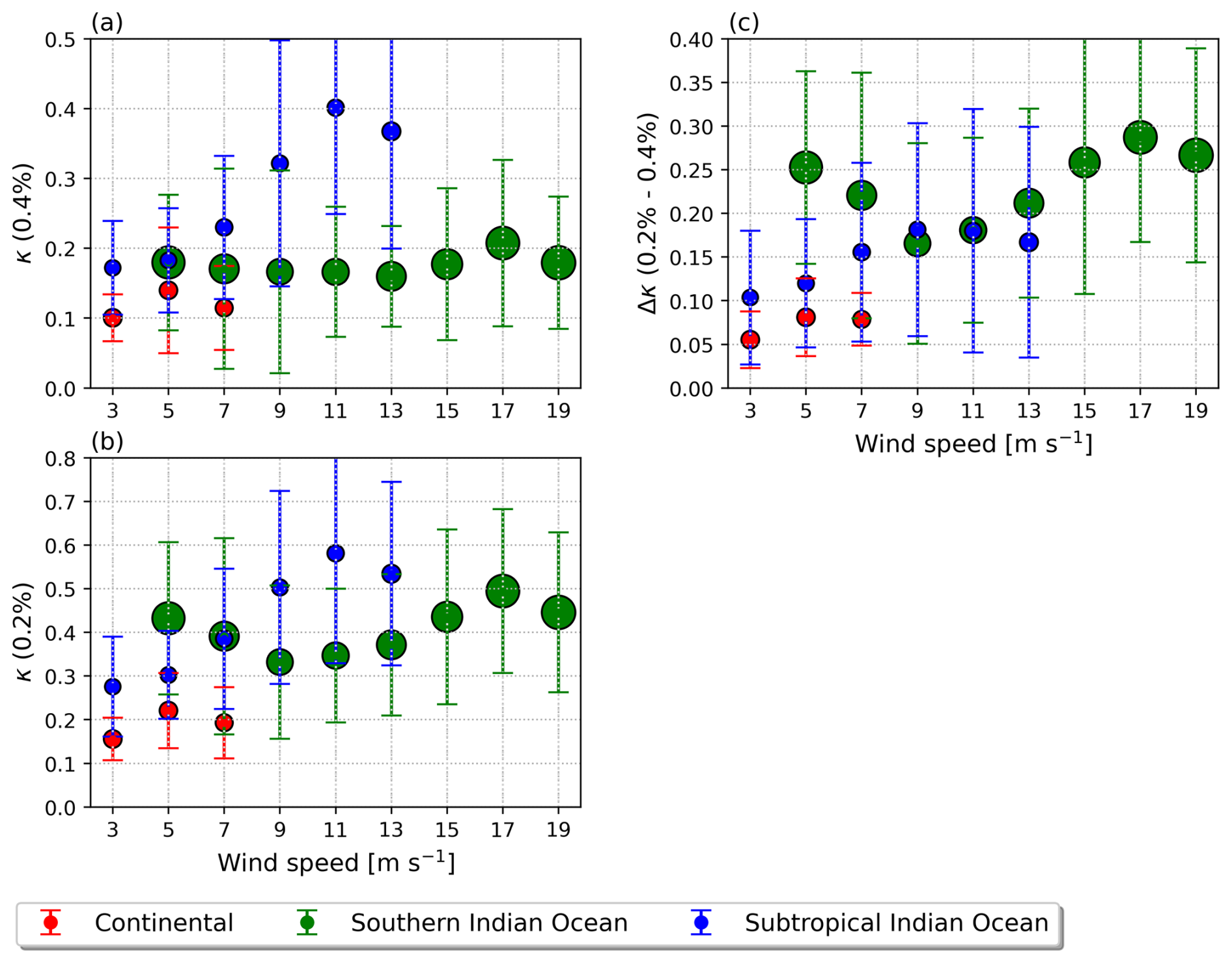
Figure 11 (a) κ at 0.4 % SS against wind speed. (b) κ at 0.2 % SS against wind speed. (c) Difference between κ at 0.2 % SS and 0.4 % SS against wind speed. The circles are the κ values averaged every 2 m s⁻¹. Nanophytoplankton abundance is proportional to the size of the circles in cells cm⁻³.

The effect of wind speed on hygroscopicity is clearly visible at both supersaturation levels for air masses from the subtropical Indian Ocean. κ values increase from 0.17 to 0.4 at 0.4 % SS (from 0.28 to 0.58 at 0.2 % SS) for wind speeds between 3 and 11 m s⁻¹. This result is consistent with the lower abundance of nanophytoplankton in this group, which makes the κ values higher than those obtained for continental and southern Indian Ocean air masses, bringing the κ values closer to those of NaCl. Δκ also increases from 0.1 to 0.18 between 3 and 9 m s⁻¹.

For air masses from the southern Indian Ocean, at 0.2 % SS, an increase in the average κ values from 0.33 to 0.5 is observed between 9 and 17 m s⁻¹. At 0.4 % SS, the κ value is stable with wind speed (∼ 0.2). The effect of the primary organic emissions in reducing the hygroscopicity, which counterbalances the increase in hygroscopicity caused by the NaCl emissions, is therefore clearly noticeable. This effect is particularly pronounced at 0.4 % supersaturation.

Δκ is higher for air masses from the southern Indian Ocean than for those from the subtropical Indian Ocean and increases with increasing wind speed between 9 and 17 m s⁻¹. Thus, a more pronounced decrease in hygroscopicity is observed for smaller aerosols, with primary emissions in regions where phytoplankton is abundant. This observation suggests the presence of a greater amount of organic matter on the surface of aerosol particles smaller than 100 nm compared to aerosols in the accumulation mode. This is consistent with the findings of Shulman et al. (1996), Oppo et al. (1999), and Facchini et al. (2008), who observed that organic surfactants tend to accumulate on the surface of aerosols. Thus, for an identical NaCl $/$ organic mass ratio, the proportion of organic matter on the surface will be greater for smaller aerosols.

7 Conclusions

This paper presents and analyzes aerosol measurements collected during six oceanographic campaigns conducted on board the Marion Dufresne in the Indian and Southern oceans in 2021 and 2023. The number of aerosols measured by the SMPS between 3 and 350 nm shows high variability, ranging from 50 to over 3000 cm⁻³. The highest concentrations (> 1000 cm⁻³) are observed in the Mozambique Channel. Back-trajectory analysis showed that this region is strongly influenced by the advection of air masses from Africa or Madagascar. These high aerosol concentrations are therefore of the same order of magnitude as those reported by Flores et al. (2020) and Koponen et al. (2002) for polluted ocean air masses. Not surprisingly, the lowest aerosol concentrations are found in the regions furthest from the continent, generally between 100 and 1000 cm⁻³.

The number of CCN at 0.4 % is much less variable, with concentrations between 60 and 500 cm⁻³ (208 cm⁻³ on average), which is similar to the observations of Sanchez et al. (2021) and Humphries et al. (2021) in the same latitudinal ranges. The difference between the number of aerosols and the number of CCN is particularly significant in the Mozambique Channel, with an $N_{\mathrm{CCN}}/N_{\mathrm{SMPS}}$ ratio of about 0.17. This ratio can be explained by the presence of more hydrophobic aerosols associated with anthropogenic pollution advection (κ < 0.1). Conversely, in regions less influenced by continental air masses, this ratio can reach 0.65 with a fairly variable hygroscopicity parameter, generally between 0.2 and 0.5, similar to the observations of Tatzelt et al. (2022).

In order to explain the variability in marine aerosol concentrations, four situations have been analyzed using back trajectories and ERA5 analyses. The first situation corresponds to the advection of a clean air mass located in the easternmost part of the measurement area. It has been observed that this type of air mass nearly evolves and that the Aitken and accumulation modes are not very pronounced. The activation diameter calculation is placed in a low-concentration range close to the instrumental noise. The calculation of the hygroscopicity parameter is therefore particularly sensitive to the consistency between the CCN-100 and SMPS measurements. The second case illustrates the high N_SMPS values above 6000 cm⁻³ recorded in northern Madagascar. These concentration peaks have been shown to originate from the layer 800 m above Madagascar, which then descends toward the Mozambique Channel. This variability has also been shown to be explained by the thickening of the mixing boundary layer in the urbanized coastal region of Madagascar, which allowed turbulent mixing of surface pollution in this upper layer. The third case corresponds to a period of storms between the Kerguelen Islands and Réunion. Paradoxically, the maximum aerosol concentration is offset from the maximum wind speed and wave height. Analysis of back trajectories and precipitation fields from the ERA5 analyses showed that during the storm passage the air mass was affected by rain, leading to a decrease in the aerosol concentration. As the ship approached Réunion and moved away from the storm, the aerosol concentrations increased to more than 3000 cm⁻³. These high concentrations were caused by the advection of an air mass that had not interacted with precipitation and had been under the influence of the storm 12 h earlier, 100 km southwest of the ship. The fourth case corresponds to a sudden increase in aerosol concentration between Réunion and the Crozet Islands. Analysis of this period revealed a nucleation event followed by particle growth, which coincided with the moment when the Marion Dufresne passed from a cloudy area to a clear-sky area. Several studies have suggested that nucleation events are rare in the marine boundary layer and generally occur in the free troposphere (Covert et al., 1996; Bates et al., 1998; Humphries et al., 2016; Sanchez et al., 2021; Schmale et al., 2019; Williamson et al., 2019). This case study is an example of a nucleation event observed in the open sea with an air mass that remained in the marine boundary layer.

To generalize these results, a series of back-trajectory simulations was made for each hour of observation. Each air mass was then separated according to its origin: continental, subtropical Indian Ocean, or southern Indian Ocean. Similar to the case studies, we find that air masses from the subtropical Indian Ocean are aged and less loaded with aerosols. This results in larger geometric diameters for the submicron modes. Conversely, air masses from the southern Indian Ocean have smaller geometric diameters, reflecting the effect of primary emissions of new particles due to stronger winds and higher wave heights. Note that the position of the submicron modes is in good agreement with the results obtained by Xu et al. (2021) and Kawana et al. (2022), who compared the size distributions of marine aerosols under polluted, clean, and marine biologically active conditions. The submicrometer aerosol size distribution of the continental group is characterized by the presence of an Aitken and an accumulation mode, in contrast to the monomodal size distribution observed by Flores et al. (2020). The number concentration of aerosols in the coarse mode is the highest for the southern Indian Ocean group and is due to a more significant primary emission production in this region.

Additionally, from this classification, we investigated the possible relationship between the wind speed, the aerosol hygroscopicity (κ), and the nanophytoplankton abundance. Continental air masses are associated with more hydrophobic aerosols (κ from 0.1 to 0.22), whereas subtropical Indian Ocean air masses are associated with more hydrophilic aerosols (κ from 0.17 to 0.6). Southern Indian Ocean air masses exhibit in-between values (κ from 0.16 to 0.5). κ values of the subtropical Indian Ocean increase when the wind speed becomes stronger (from 3 to 11 m s⁻¹). These results show the effect of primary organic emissions on the decrease in κ in areas characterized by high phytoplankton concentrations, which counterbalances the increase in κ caused by NaCl emissions. This is consistent with previous studies highlighted by O'Dowd et al. (2004) and Schwier et al. (2015). A significant decrease in κ (between 0.2 % and 0.4 % supersaturation) when the wind speed increases from 9 to 17 m s⁻¹ is observed for air masses originating from the southern Indian Ocean. This phenomenon can be ascribed to the presence of a heightened concentration of organic species on the surface of smaller aerosols, which consequently leads to a reduction in the hygroscopic parameter.

This paper offers a large overview of the diversity of marine aerosols present in the subtropical and southern Indian Ocean, highlighting the variability in their hygroscopicity and CCN properties. This diversity was revealed through measurements taken over an extended period and under various environmental conditions, thus confirming the value of the MAP-IO program. These preliminary results can be further investigated over the course of several years as the program's database expands, enabling the characterization of the intraseasonal variability in marine aerosol properties. This paper highlights the need to incorporate the variability in marine aerosol CCN properties into meteorological models, emphasizing the complexity of their characterization due to various coupled processes involving emissions, transport, aging, and chemical composition. Introducing this variability would enable the cloud life cycle to be parameterized more accurately in meteorological models, particularly with regard to droplet size distribution and precipitation formation.

Appendix A: Air mass classification

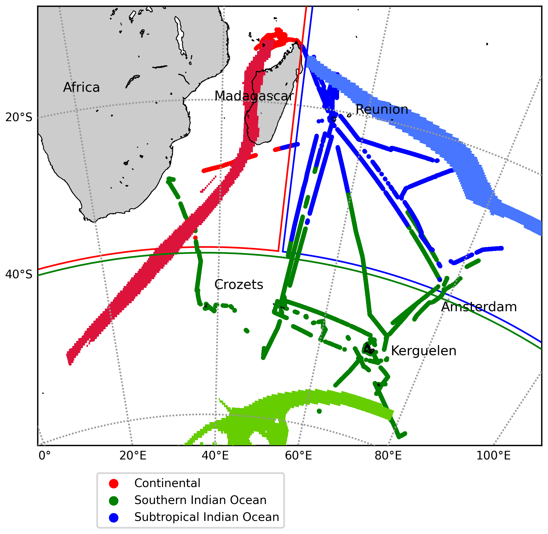
Figure A1 Classification of the aerosol data recorded in 2021 and 2023 according to the 5 d back trajectories simulated by the FLEXPART model. Back trajectories in red, blue, and green are examples of continental, subtropical Indian Ocean, and southern Indian Ocean air masses.