the Creative Commons Attribution 4.0 License.
the Creative Commons Attribution 4.0 License.
 | 09 Sep 2024
Global assessment of climatic responses to ozone–vegetation interactions
Xinyi Zhou
Chenguang Tian
Xiaofei Lu
The coupling between surface ozone (O3) and vegetation significantly influences the regional to global climate. O3 uptake by plant stomata inhibits the photosynthetic rate and stomatal conductance, impacting evapotranspiration through land surface ecosystems. Using a climate–vegetation–chemistry coupled model (the NASA GISS ModelE2 coupled with the Yale Interactive terrestrial Biosphere, or ModelE2-YIBs), we assess the global climatic responses to O3–vegetation interactions during the boreal summer of the present day (2005–2014). High O3 pollution reduces stomatal conductance, resulting in warmer and drier conditions worldwide. The most significant responses are found in the eastern US and eastern China, where the surface air temperature increases by +0.33 ± 0.87 and +0.56 ± 0.38 °C, respectively. These temperature increases are accompanied by decreased latent heat and increased sensible heat in both regions. The O3–vegetation interaction also affects atmospheric pollutants. The surface maximum daily 8 h average O3 concentrations increase by +1.46 ± 3.02 ppbv in eastern China and +1.15 ± 1.77 ppbv in the eastern US due to the O3-induced inhibition of stomatal uptake. With reduced atmospheric stability following a warmer climate, increased cloud cover but decreased relative humidity jointly reduce aerosol optical depth by −0.06 ± 0.01 (−14.67 ± 12.15 %) over eastern China. This study suggests that vegetation feedback should be considered for a more accurate assessment of climatic perturbations caused by tropospheric O3.
- Article
(6560 KB) - Full-text XML
-
Supplement
(4417 KB) - BibTeX
- EndNote


Tropospheric ozone (O3), one of the most detrimental air pollutants (Myhre et al., 2013), not only threatens human health (Norval et al., 2011; Nuvolone et al., 2018) but also induces phytotoxic effects on vegetation (Mills et al., 2007; Pleijel et al., 2007). When plants are exposed to certain levels of O3, plant photosynthesis and stomatal conductance are inhibited because of the O3 oxidation of cells, enzymes, and chlorophyll (Dizengremel, 2001; Fiscus et al., 2005; Jolivet et al., 2016). Consequently, carbon assimilation in terrestrial ecosystems is limited (Yue and Unger, 2014; Oliver et al., 2018), and the land–air exchange rates of water and heat fluxes are altered (Lombardozzi et al., 2015).
Experimental studies have shown that excessive O3 exposure reduces both plant photosynthesis and stomatal conductance (Ainsworth et al., 2012; Lombardozzi et al., 2013). The reduction rates are dependent on the O3 stomatal fluxes and the damage sensitivities, which vary among different vegetation types (Nussbaum and Fuhrer, 2000; Karlsson et al., 2004; Pleijel et al., 2004). Several exposure-based indices, such as accumulated hourly O3 concentrations over a threshold of 40 ppb (AOT40) and the sum of all hourly average concentrations (SUM00), are used to assess O3-induced vegetation damage (Fuhrer et al., 1997; Paoletti et al., 2007). In addition, the flux-related PODy method (phytotoxic O3 dose above a threshold flux of y) is also widely applied to consider the dynamic adjustment of stomatal conductance (Buker et al., 2015; Sicard et al., 2016). Considering the variability of plant sensitivities, different O3 damage schemes have been proposed to quantify the impacts of O3 on land carbon assimilation at regional to global scales (Anav et al., 2011; Lam et al., 2023; Lei et al., 2020). For example, Sitch et al. (2007) calculated simultaneous damage to both photosynthesis and stomatal conductance on the basis of instantaneous O3 stomatal uptake. In contrast, Lombardozzi et al. (2012) estimated decoupled reductions in plant photosynthesis and stomatal conductance via different response relationships to cumulative O3 stomatal uptake. The application of different schemes has resulted in a wide range of reductions in gross primary productivity (GPP) of 2 %–12 % globally, with regional hotspots of up to 20 %–30 % (Lombardozzi et al., 2015; Unger et al., 2020; Zhou et al., 2024).
O3-induced inhibition of stomatal conductance decreases dry deposition and consequently enhances surface O3 concentrations (Clifton et al., 2020; Wesely and Hicks, 2000; Zhang et al., 2006). Using the Sitch et al. (2007) scheme with high O3 damage sensitivities in ModelE2-YIBs (NASA GISS ModelE2 coupled with the Yale Interactive terrestrial Biosphere model), Gong et al. (2020) revealed that O3–vegetation interactions increased regional O3 concentrations by 1.8 ppbv in the eastern US, 1.3 ppbv in Europe, and 2.1 ppbv in eastern China in 2010. In comparison, Sadiq et al. (2017) reported consistently stronger feedbacks on O3 concentrations in these polluted regions via the scheme of Lombardozzi et al. (2012) embedded in the Community Earth System Model (CESM). Moreover, the inclusion of online O3–vegetation interactions in numerical models will also result in a greater loss of simulated land carbon assimilation due to the feedbacks of both ecosystems and surface O3. This is attributable to several factors. On the one hand, O3 damage to leaf photosynthesis inhibits plant growth and decreases the leaf area index (LAI), leading to a greater reduction in GPP than in simulations without LAI changes (Yue et al., 2020). On the other hand, O3 enhancement due to vegetation feedback may cause additional vegetation damage and result in further GPP losses (Lei et al., 2021). As a result, O3–vegetation interactions should be considered in global estimates of O3 damage to ecosystem functions.
In addition to affecting surface O3, O3–vegetation interactions can also alter water and energy exchanges between the land and atmosphere through the modulation of stomatal conductance. For example, Lombardozzi et al. (2015) used the Community Land Model (CLM) and estimated that the cumulative uptake of O3 by leaves resulted in a reduction of 2.2 % in transpiration but an increase of 5.4 % in runoff globally. Arnold et al. (2018) used CESM and reported that plant exposure to O3 could decrease land–air moisture fluxes and atmospheric humidity, which would further reduce shortwave cloud forcing in polluted regions and induce widespread surface warming up to +1.5 K. Two recent studies utilized the WRF-Chem model and revealed considerable warming and associated meteorological perturbations due to O3–vegetation interactions in China (Zhu et al., 2022; Jin et al., 2023). However, all these modeling studies applied the same O3 vegetation damage scheme proposed by Lombardozzi et al. (2012). It is necessary to assess the climatic responses to O3–vegetation interactions via different schemes to explore robust responses and associated uncertainties.
In this study, we quantified the global impacts of O3–vegetation interactions on climatic conditions and surface air pollutants during the 2010s using ModelE2-YIBs (Yue and Unger, 2015). This fully coupled framework was implemented with the semi-mechanistic O3 damage scheme proposed by Sitch et al. (2007), which calculates aggregated O3 damage to photosynthesis on the basis of varied sensitivities to instantaneous stomatal O3 uptake across eight plant functional types (PFTs). We performed sensitivity experiments to quantify the responses of surface air temperature and precipitation to O3–vegetation interactions. The feedbacks to aerosols and O3 concentrations were also examined.
2.1 Model descriptions
ModelE2-YIBs is a fully coupled climate–carbon–chemistry model that combines the NASA GISS ModelE2 with the YIBs vegetation model. ModelE2 is a general circulation model with a horizontal resolution of 2° × 2.5° in latitude and longitude and 40 vertical layers up to 0.1 hPa. It dynamically simulates gas-phase chemistry (NOx, HOx, Ox, CO, CH4, and non-methane volatile organic compounds (NMVOCs)), aerosols (sulfate, nitrate, black and organic carbon, dust, and sea salt), and their interactions (Menon and Rotstayn, 2006). Both the physical and chemical processes are calculated every 0.5 h, and the radiation module is called every 2.5 h. The radiation module includes direct and indirect aerosol radiative effects and accounts for the absorption of multiple greenhouse gases (GHGs). For cloud optical parameters, Mie scattering, ray tracing, and matrix theory are used (Schmidt et al., 2006). The model outperforms 20 other IPCC-class climate models in simulating surface solar radiation (Wild et al., 2013) and has been extensively validated for meteorological and hydrological variables against observations and reanalysis data (Schmidt et al., 2014).
The YIBs model employs the well-established Farquhar model for leaf photosynthesis and the Ball–Berry model for stomatal conductance (Farquhar et al., 1980; Ball et al., 1987) as follows:
Here, the total leaf photosynthesis, denoted as Atot (), is calculated considering both C3 (Collatz et al., 1991) and C4 plants (Collatz et al., 1992). Atot is derived from the minimum value of the constraints. The rate of carboxylation limited by ribulose-1,5-bisphosphate carboxylase (Rubisco) is Jc:
The carboxylation rate restricted by the availability of light is Je:
The export-limited rates for C3 plants and the phosphoenolpyruvate carboxylase (PEPC)-limited rates of carboxylation for C4 plants are represented by Js:
In these functions, Vcmax () is the maximum carboxylation capacity. ci and Oi (Pa) represent the internal leaf CO2 and oxygen partial pressure, respectively. Γ∗ (Pa) denotes the CO2 compensation point, whereas Kc and Ko (Pa) are Michaelis–Menten constants for the carboxylation and oxygenation of Rubisco, respectively. The parameters Γ∗, Kc, and Ko vary with temperature on the basis of the sensitivity of the vegetation to temperature (Q10 coefficient). PAR () is the absorbed photosynthetically active radiation, aleaf is the leaf-specific light absorbance that considers sunlit and shaded leaves, and α is the quantum efficiency. Patm (Pa) represents the ambient pressure. Ks is set to 4000 as a constant following Oleson et al. (2010) to limit photosynthesis to C4 plants that become saturated at lower CO2 concentrations.
The stomatal conductance (gs, ) is linked to the variations in Atot, with several parameters, such as the dark respiration rate (Rd, ), relative humidity (RH), and CO2 concentration at the leaf surface (cs):
The model simulates the biophysical processes of eight PFTs, including tundra, C3 and/or C4 grass, shrubland, deciduous broadleaf forest, evergreen broadleaf forest, evergreen needleleaf forest, and cropland. Different values are assigned to parameters m and b for each PFT (Table S1 in the Supplement). The carbon taken up by the leaf then accumulates and is allocated to different organs to support plant development, resulting in dynamic changes in the LAI and tree growth.
2.2 O3–vegetation damage scheme
The YIBs model employs a semi-mechanistic parameterization proposed by Sitch et al. (2007) to estimate the impact of O3 on photosynthesis through stomatal uptake. The scheme applies an undamaged factor (F) () to calculate both Atot and gs as follows:
where Atotd and gsd are the unaffected photosynthesis and stomatal conductance, respectively. The factor F is defined as follows:
where ah () is the high O3 sensitivity coefficient, calibrated by Sitch et al. (2007) on data from field observations by Karlsson et al. (2004) and Pleijel et al. (2004) to represent the “high” sensitivity of the relative species of each PFT. () is the specific threshold for O3 damage. Both ah and vary with vegetation types (Table S1):
where [O3] represents surface O3 concentrations, and Ra (s m−1) represents aerodynamic resistance, which expresses the turbulent transport efficiency in transferring sensible heat and water vapor between the land surface and a reference height. The constant = 1.67 is the ratio of stomatal resistance to O3, which is estimated on the basis of the theoretical stomatal resistance to water (Laisk et al., 1989). When plants are exposed to [O3] (Eq. 9), Atot and gs decrease (Eqs. 6 and 7) if the excess O3 enters the leaves (Eq. 8). The increased stomatal resistance protects plants by reducing the O3 uptake of stomata. Consequently, the damage scheme describes changes in both the photosynthetic rate and stomatal conductance.
2.3 Experiments
To explore the coupled O3–vegetation effect, we performed two simulations using the ModelE2-YIBs model. The control experiment, O3_offline, was conducted without O3 damage to vegetation. For comparison, the sensitivity experiment, O3_online, included online O3–vegetation interactions with high O3 sensitivity. For both experiments, the anthropogenic emissions from 2010 (the average of 2005–2014) of eight species (BC, OC, CO, NH3, NOx, SO2, alkenes, and paraffin) from eight economic sources (agriculture, energy, industry, transportation, residential, solvent, waste, and international shipping) and biomass burning sources were collected from the Coupled Model Intercomparison Project phase 6 (CMIP6) (van Marle et al., 2017; Hoesly et al., 2018). The ensemble means of the monthly sea surface temperature (SST) and sea ice concentration (SIC) simulated by 21 CMIP6 models during the time period of 2005–2014 were employed as the boundary conditions. The cover fractions of eight PFTs (Fig. S1 in the Supplement) fixed in 2010 were adopted from the land use harmonization (LUH2) dataset (Hurtt et al., 2020). For each time slice simulation, the model was run for 30 years with all the input data fixed, and the first 10 years were used as the spin-up period. We calculated the average of the last 20 years and focused on the boreal summer season (June–July–August, JJA), when the interaction of vegetation and surface O3 reaches its annual maximum (Fig. S3). To show the uncertainty introduced by the internal variability of the model, all the related global and regional values are denoted as mean/sum ± standard deviation of the last 20 model years. We explored the climatic responses to O3–vegetation interactions as the differences between O3_online and O3_offline at the global scale, with a focus on hotspot regions, such as the eastern US (30–40° N, 80–90° W) and eastern China (22.5–38° N, 106–122° E).
2.4 Data for model evaluation
We evaluated the simulated air pollutants, carbon fluxes, and meteorological variables from the O3_offline simulation against observational and reanalysis datasets. The worldwide observations of the maximum daily 8 h average O3 (MDA8 O3) concentrations were collected from three regional networks: the Air Quality Monitoring Network operated by the Ministry of Ecology and Environment (AQMN-MEE) in China, the Clean Air Status and Trends Network (CASTNET) in the US, and the European Monitoring and Evaluation Programme (EMEP) in Europe. The observations used for validation beyond China, sourced from Sofen et al. (2016), are averaged over the period 2005–2014. This dataset encompasses 7288 station records worldwide and excludes the uncertainty associated with high mountaintop sites. For AQMN-MEE, the mean value of 2014–2018 was used because it was established in 2013. The simulated aerosol optical depth (AOD) and LAI were validated using satellite-based data from the moderate-resolution imaging spectroradiometer (MODIS) retrievals collection 5 (Remer et al., 2005) (http://modis.gsfc.nasa.gov/, last access: 5 August 2022) averaged over the years 2005–2014. The simulated GPP was evaluated against the data product upscaled from the FLUXNET eddy covariance measurements for 2009–2011 (Jung et al., 2011). The daily temperature at 2 m (T2 m) from 2005 to 2014 was obtained from the National Centers for Environmental Prediction/National Center for Atmospheric Research (NCEP/NCAR) reanalysis 1 (NCEP1) (Kalnay et al., 1996). For precipitation, we used the monthly data averaged from 2005 to 2014 from the Global Precipitation Climatology Project (GPCP) (Huffman et al., 1997; Adler et al., 2018). All these datasets were interpolated to the same resolution as the ModelE2-YIBs model. The root-mean-square error (RMSE) and normalized mean bias (NMB) were applied to quantify the deviations of the simulations from the observations:
Here, Si and Oi represent the simulated and observed values, respectively, and n denotes the total number of grid points used in the comparisons.
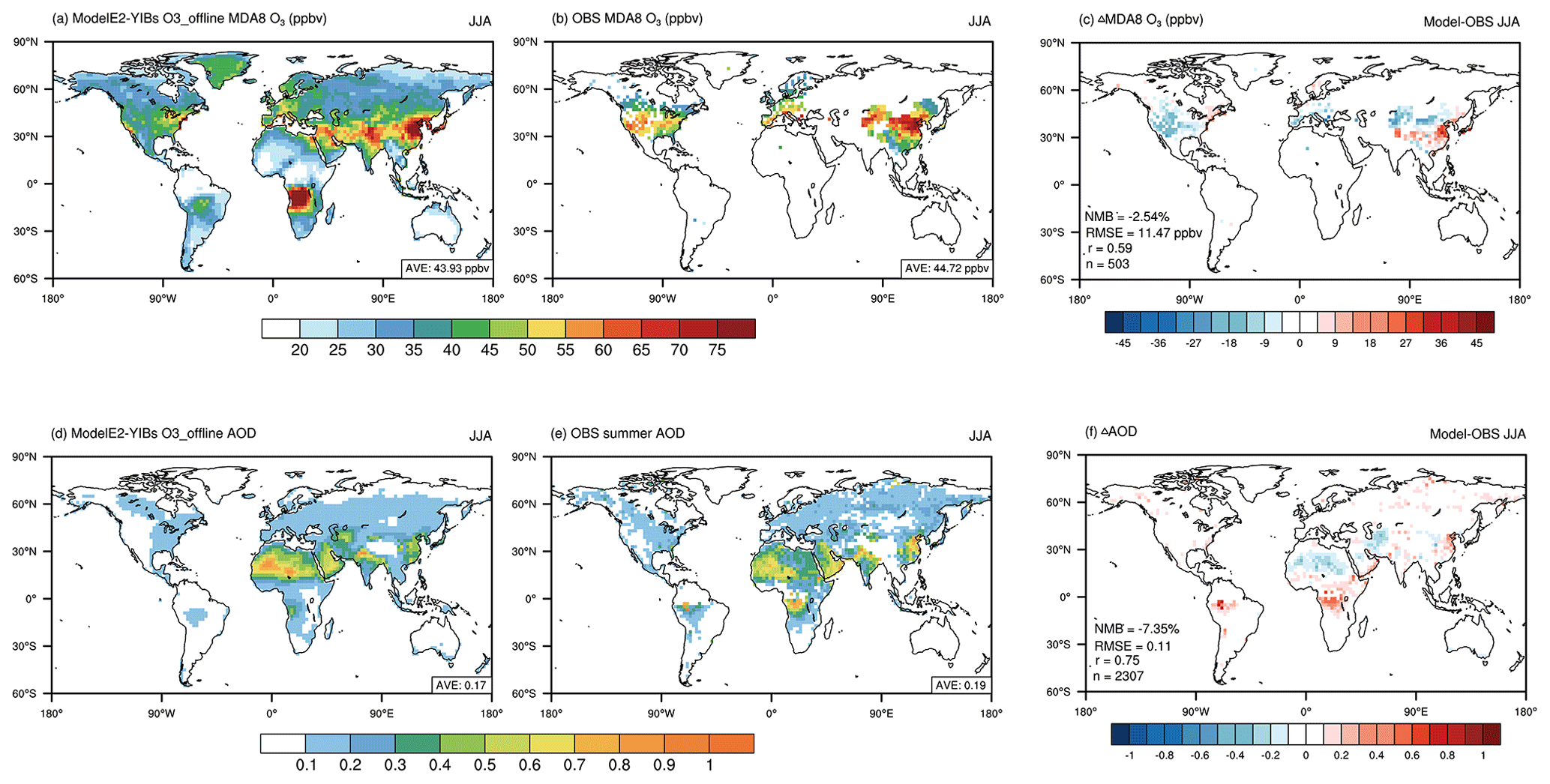
Figure 1Evaluation of the present-day boreal summertime (June–August) air pollutants simulated by the ModelE2-YIBs model. The MDA8 O3 (a–c) and AOD (d–f) from the O3_offline simulation (a, d) and observations (b, e) are compared. The correlation coefficient (r), root-mean-square error (RMSE), normalized mean bias (NMB), and number of grid cells (n) for the comparisons are listed on the mean bias maps (c, f).
3.1 Control simulation and model evaluations
We first evaluated the air pollutants simulated by the control simulation (O3_offline) of the ModelE2-YIBs model (Fig. 1). Over a total of 503 grids with site-level O3 measurements (Fig. 1b), the model replicated both the magnitude and spatial distribution of MDA8 O3, with a correlation coefficient (r) of 0.59 and an NMB of −2.54 % (Fig. 1c). The simulated summertime surface MDA8 O3 concentration was high in regions with high anthropogenic emissions, such as western Europe and eastern China (Ohara et al., 2007), as well as in central Africa, which has frequent fire emissions (van der Werf et al., 2017). At the global scale, the model yielded an average MDA8 O3 concentration of 43.93 ppbv, and observations revealed an average of 44.72 ppbv over the same grids. However, the model overestimated the concentrations over the North China Plain and slightly underestimated them over the US, likely due to biases in the emission inventories and the predicted climate that drive O3 production. The AOD simulated at 550 nm by O3_offline (Fig. 1d) showed a spatial pattern similar to that of the satellite retrievals (Fig. 1e), with r = 0.75 and an NMB of −7.35 % globally (Fig. 1f). Both simulations and observations revealed AOD hotspots over northern Africa and the Middle East, where dust emissions dominate, and in northern India and eastern China, where anthropogenic emissions are high (Feng et al., 2020).
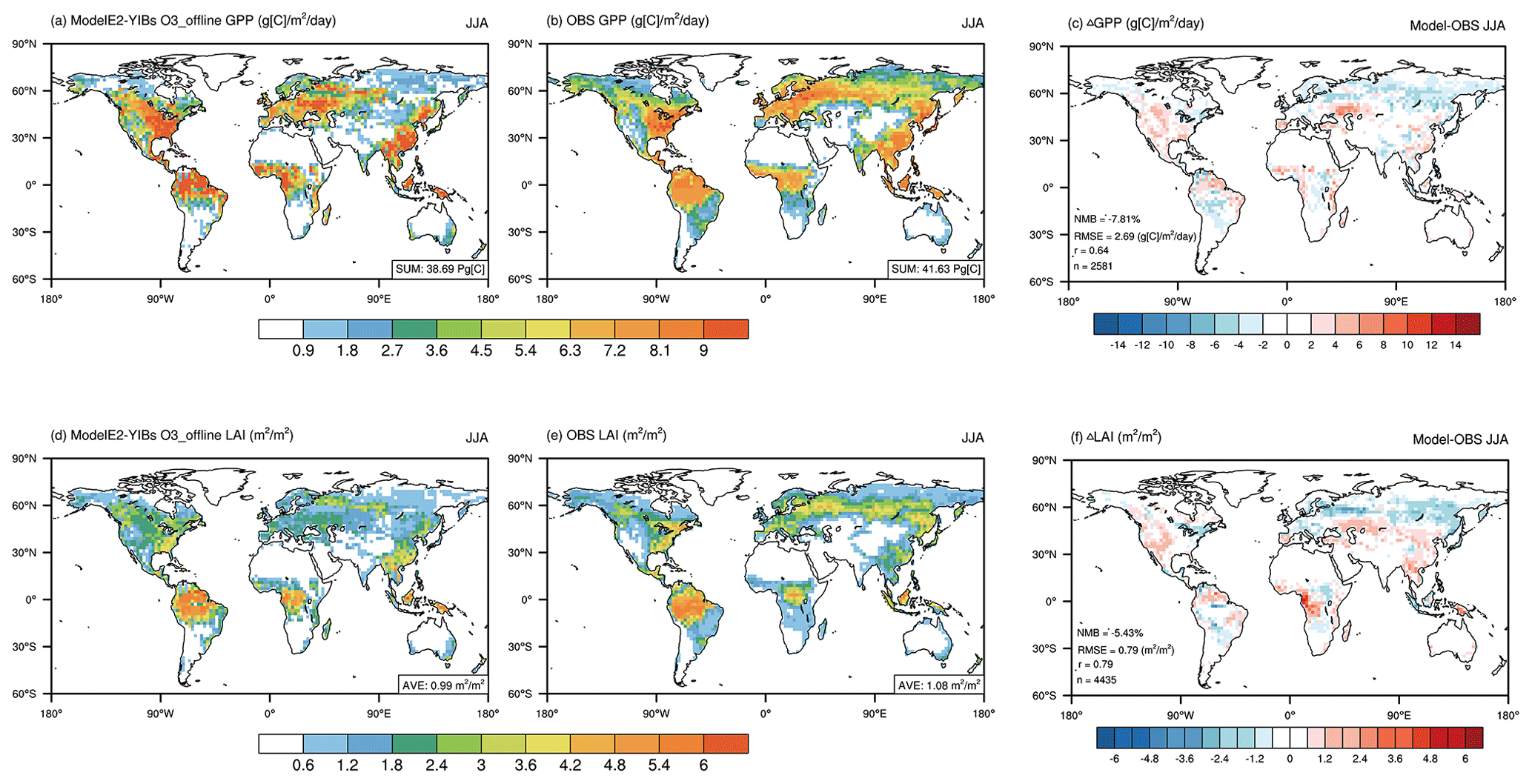
Figure 2Same as in Fig. 1 but for gross primary productivity (GPP; a–c) and the leaf area index (LAI; d–f).
We then evaluated the simulated GPP and LAI via a control experiment for the boreal summer period (Fig. 2). The observations revealed GPP hotspots over boreal forests, such as those in the eastern US, Eurasia, and East Asia, and over tropical forests, such as those in the Amazon, central Africa, and Indonesia (Fig. 2b). The seasonal total GPP was estimated to be 41.63 Pg [C], which accounted for 35 % of the annual amount. The simulations captured the observed GPP pattern at the global scale, with r = 0.64 and NMB = −7.81 % across 2581 grids (Fig. 2c), with underestimations in the tundra area and slight overestimations in the tropical-rainforest and evergreen-forest regions. The model simulated a seasonal total GPP of 38.69 Pg [C], equivalent to 34 % of the annual amount. The simulated LAI showed patterns similar to those of GPP (Fig. 2d) and resembled the observed LAI (Fig. 2e), with a spatial correlation of r = 0.79 and a low NMB = −5.43 % across 4435 grids globally (Fig. 2f).
We further validated the simulated meteorology from O3_offline (Fig. S2). For the surface air temperature, the model (Fig. S2a) reproduced the observed (Fig. S2b) pattern, with an RMSE of 3.21 °C and an r of 0.99 compared with the observations (Fig. S2c). For precipitation, the simulation (Fig. S2d) captured the observed spatial pattern (Fig. S2e), with NMB = 17.26 % and r = 0.75 (Fig. S2f). Overall, the model captured the spatial characteristics and magnitudes of air pollutants, biospheric parameters, and meteorological fields, making it a valuable tool for studying O3–vegetation interactions.
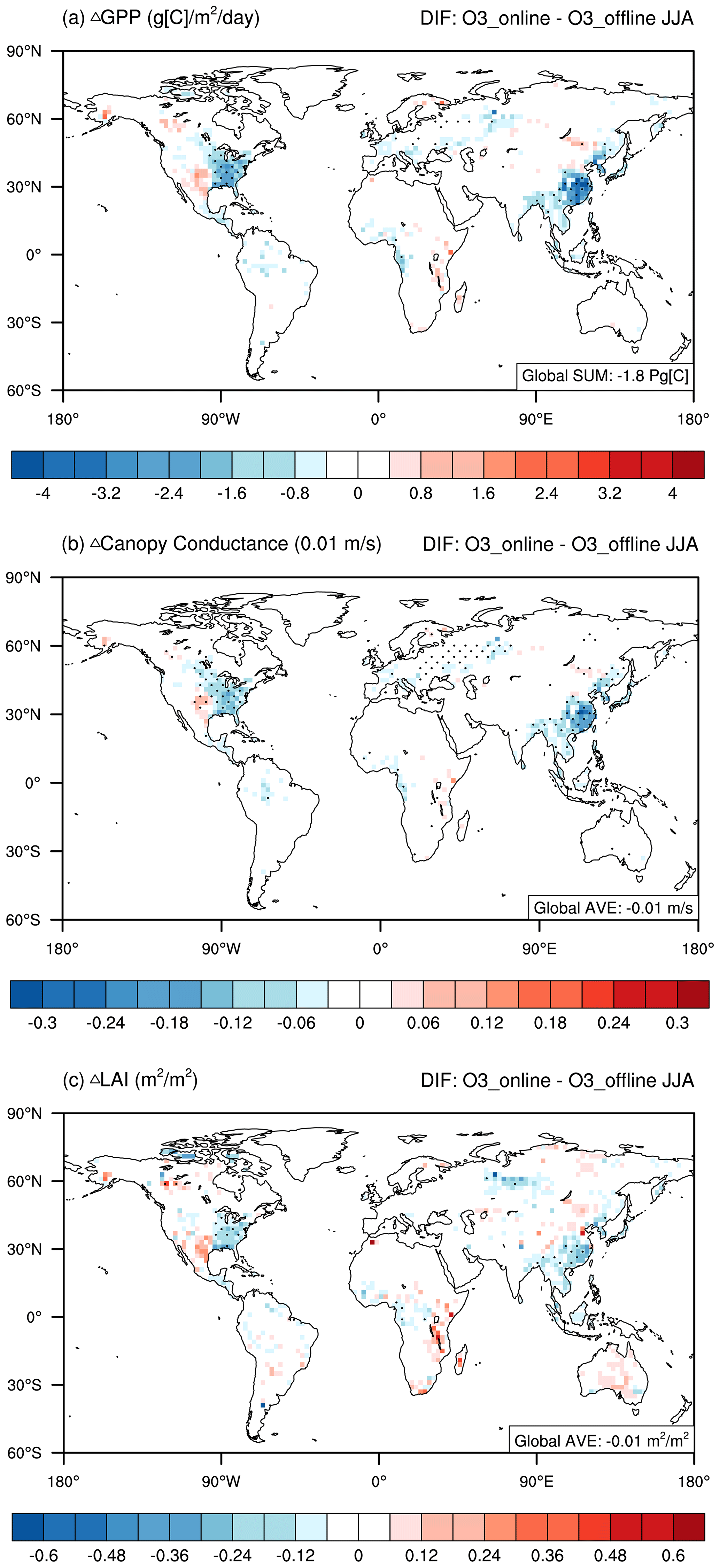
Figure 3Changes in present-day boreal-summertime biospheric variables induced by O3–vegetation interactions. The results shown are the changes in (a) GPP, (b) canopy conductance, and (c) LAI between the O3_online and O3_offline simulations. The black dots denote areas with significant changes (p < 0.1).
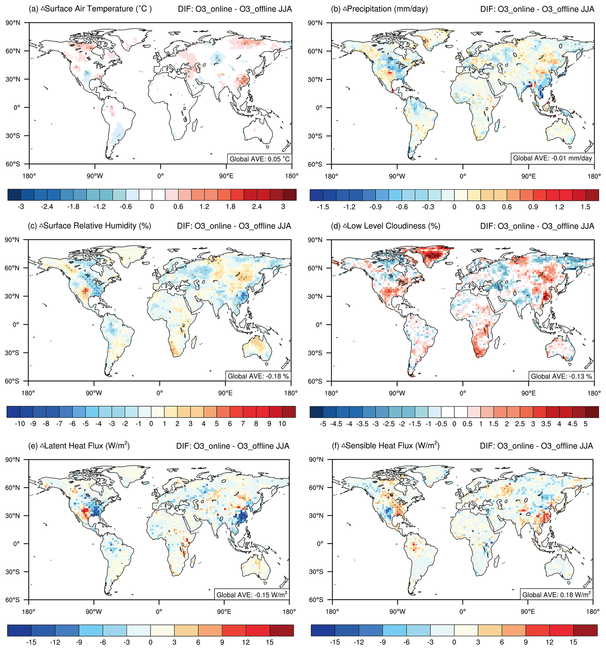
Figure 4Changes in present-day boreal-summertime meteorological fields caused by O3–vegetation interactions. The results shown are changes in (a) surface air temperature, (b) precipitation, (c) surface relative humidity, (d) low-level cloudiness, (e) latent heat flux, and (f) sensible heat flux between the O3_online and O3_offline simulations. For heat fluxes, positive values (shaded in red) indicate that the upward fluxes change. The black dots denote areas with significant changes (p < 0.1).
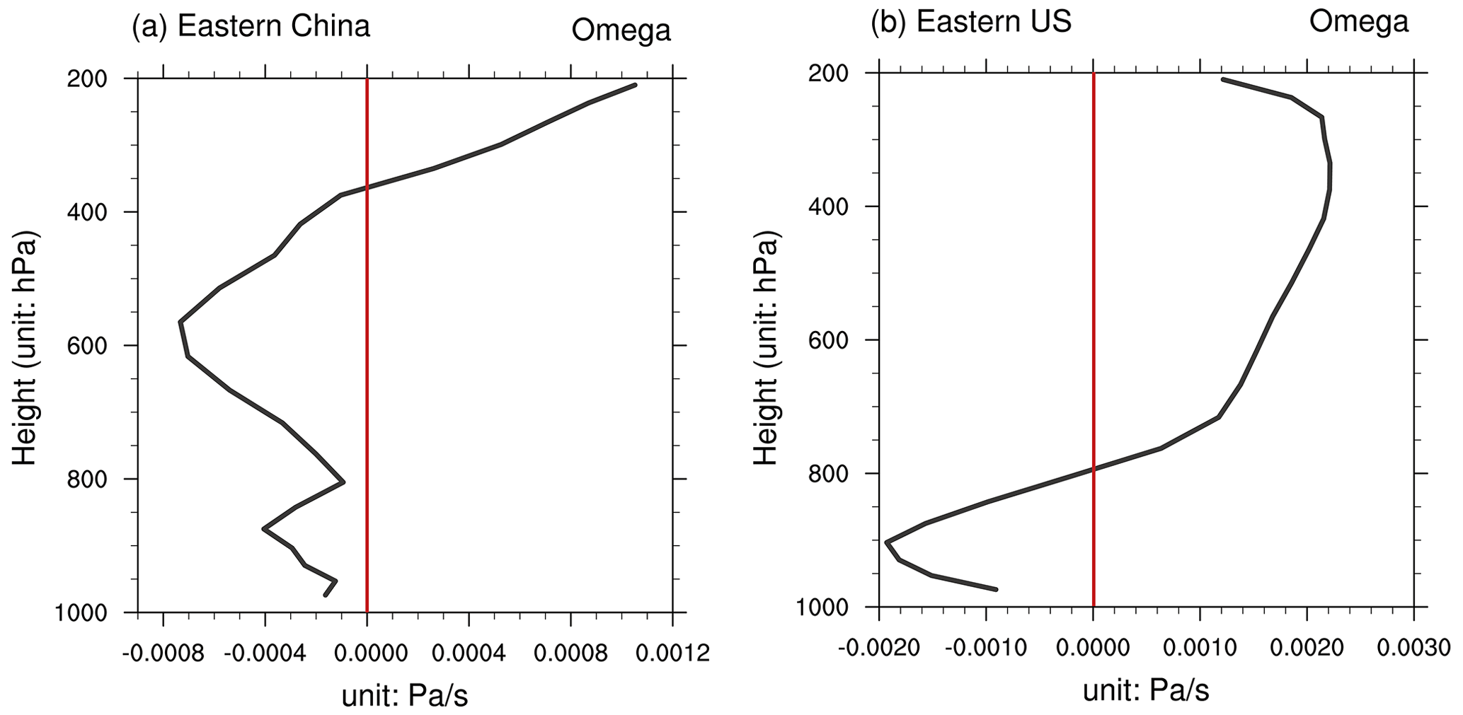
Figure 5Vertical profile of the vertical velocity. The results shown are changes in the vertical velocity in (a) eastern China and (b) the eastern US between the O3_online and O3_offline simulations. The solid red line denotes 0. Please note the differences in the scales.
3.2 O3 damage to terrestrial ecosystems
We assessed the damaging effects of surface O3 on ecosystems due to online O3–vegetation interactions (Fig. 3). The impacts of O3 on biospheric variables were mainly located in regions characterized by abundant vegetation cover and elevated O3 concentrations. On the global scale, O3 induced a GPP reduction of −1.80 ± 0.61 Pg C yr−1 (−4.69 ± 1.56 %, Fig. 3a). This deleterious effect was more pronounced in specific regions, notably eastern China and the eastern US, with significant GPP declines of −25.40 ± 1.90 % and −20.14 ± 5.02 %, respectively, under conditions of high O3 sensitivity (Fig. 3a and Table S2). Moreover, stomatal conductance significantly decreased in the middle latitudes of the Northern Hemisphere (Fig. 3b). The most substantial relative change of −30.62 ± 4.30 % was observed in eastern China, followed by −25.65 ± 9.32 % in the eastern US (Fig. 3b and Table S2). Although there are positive responses in some regions, they are not dominant and are hardly significant. These values were stronger than those for GPP (Fig. 3a), likely because of the climatic feedback to O3–vegetation interactions. The opening of the plant stoma plays a crucial role in regulating energy and water exchange between the land surface and the atmosphere. The inhibition of stomatal conductance by surface O3 leads to a warmer (Fig. 4a) and drier (Fig. 4b) climate in those hotspot regions, resulting in even stronger inhibitory effects on stomatal conductance. Following the changes in GPP, the global LAI decreased by, on average, 0.01 ± 0.01 m2 m−2 (−0.62 ± 0.84 %), with regional maxima of −4.53 ± 1.14 % in eastern China and −5.87 ± 3.11 % in the eastern US (Table S2).
3.3 Global climatic responses to O3–vegetation interactions
In response to the O3-induced inhibition of stomatal conductance, surface air temperature increased by 0.05 ± 0.20 °C (Fig. 4a), whereas precipitation decreased by −0.01 ± 0.03 mm d−1 (Fig. 4b) at the global scale. The most significant change was the warming of 0.56 ± 0.38 °C and the precipitation reduction of −0.79 ± 1.05 mm d−1 (−16.18 ± 20.38 %) in eastern China (Table S3), followed by the greatest inhibition of stomatal conductance (Fig. 3b). Such warming and rainfall deficits also appeared in the eastern US and western Europe, where the O3–vegetation interactions were notable. The O3-induced inhibition of stomatal conductance decreased the latent heat flux (Fig. 4e) and consequent precipitation (Fig. 4b) in those hotspot regions. Moreover, the reduced latent heat flux promoted higher surface air temperatures (Fig. 4a), resulting in an increase in the sensible heat flux (Fig. 4f). Such warming has also been reported in field experiments, where relatively high O3 exposure resulted in noticeable increases in canopy temperature, along with reductions in transpiration (Bernacchi et al., 2011; VanLoocke et al., 2012). Globally, temperature and precipitation showed patchy responses with both positive and negative anomalies, suggesting that the regional hotspots of O3-induced meteorological changes propagate to surrounding areas through atmospheric perturbations.
We further examined the changes in air humidity and cloud cover. The surface relative humidity decreased by −0.18 ± 0.53 % globally, with a similar pattern to that of precipitation (Fig. 4c). The most significant reductions occurred over eastern China and the eastern US, where both warming (Fig. 4a) and rainfall deficits (Fig. 4b) contributed to drought. However, in adjacent regions, such as northern China and the central US, both rainfall and surface relative humidity increased. These changes were associated with the regional increase in cloud cover (Fig. 4d). The sensible heat flux increased by 6.3 ± 5.4 W m−2 (16.54 ± 15.59 %) and 7.12 ± 3.86 W m−2 (25.46 ± 14.71 %) in the eastern US and eastern China, respectively, suggesting the transfer of thermal energy from the land to the atmosphere via O3–vegetation interactions (Fig. 4f and Table S3). The warming effect further triggered anomalous updrafts in the lower troposphere, represented by changes in vertical velocity (Fig. 5), leading to enhanced convection; reduced atmospheric stability; and, consequently, an increase in low-level cloud cover (Fig. 4d). However, despite the usual cooling effect associated with increased cloud cover due to reductions in radiation, in regions predominantly influenced by O3–vegetation interactions, this cooling effect was outweighed by O3-induced warming through the inhibition of stomatal conductance. Therefore, temperatures exhibited an overall increase of 0.56 ± 0.38 °C in eastern China and 0.33 ± 0.87 °C in the eastern US (Table S3).
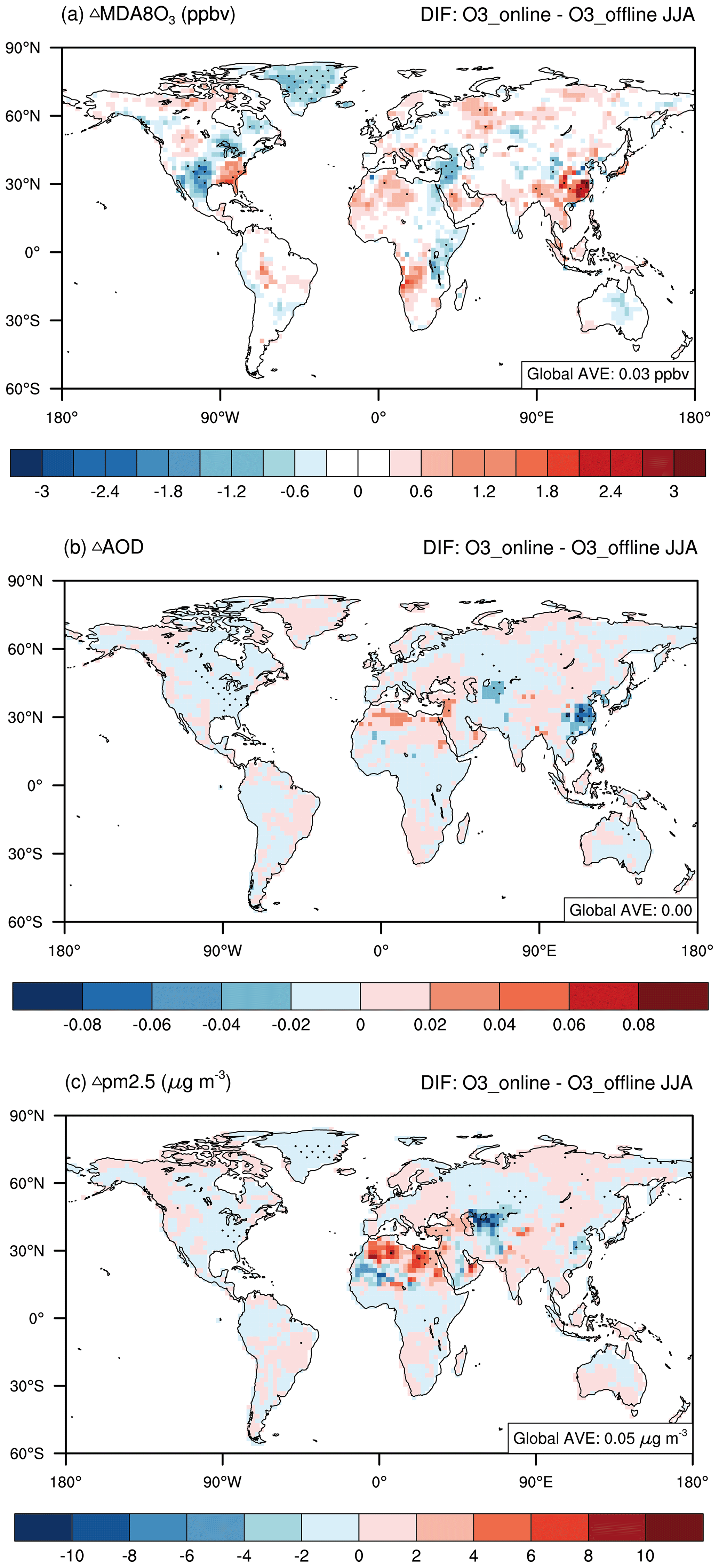
Figure 6Changes in present-day summertime atmospheric pollution caused by O3–vegetation interactions. The results shown are the changes in (a) O3, (b) AOD, and (c) PM2.5 between the O3_online and O3_offline simulations. The black dots denote areas with significant changes (p < 0.1).
3.4 Changes in air pollution caused by O3–vegetation interactions
Changes in surface water and heat fluxes induced by O3–vegetation interactions could feed back to affect air pollutants, such as O3 and aerosols. As shown in Fig. 6a and Table S4, surface MDA8 O3 concentrations increased by 1.46 ± 3.02 ppbv in eastern China and 1.15 ± 1.77 ppbv in the eastern US due to decreased dry deposition following O3 inhibition of stomatal conductance. This indicates that high contemporary O3 pollution may worsen air quality through O3–vegetation interactions. However, negative O3 changes were predicted in the central US and western China, where increased rainfall dampened O3 through chemical reactions and wet deposition. On a global scale, surface MDA8 O3 concentrations showed a limited increase of 0.03 ± 0.4 ppbv because of the offset between positive and negative feedbacks. The increase in O3 concentrations in polluted regions may exacerbate the warming effect of O3 as a greenhouse gas and may cause additional damage to vegetation. For example, the effects of offline O3 damage on GPP in eastern China and the eastern US were simulated to be −0.52 ± 0.03 Pg [C] (−24.98 ± 0.91 %) and −0.17 ± 0.02 Pg [C] (−16.71 ± 1.16 %), respectively, which are smaller than those induced by O3–vegetation interactions (Table S2).
Aerosols also exhibited evident changes in response to O3–vegetation interactions. The AOD significantly decreased over hotspot regions, such as eastern China and the eastern US (Fig. 6b). In the ModelE2-YIBs model, sulfate was especially sensitive to clouds, which could enhance aerosol scavenging through cloud water precipitation (Koch et al., 2006). The large increase in cloud cover removed sulfate more efficiently than the other aerosol species did, leading to an average decrease of −1.94 ± 1.67 µg m−3 (−8.52 ± 6.88 %) in the PM2.5 loading over eastern China (Fig. S4 and Table S4). Moreover, the reduction in surface relative humidity (Fig. 4c) in the regions with strong O3–vegetation interactions limited the hygroscopic growth of aerosols, leading to a more noticeable decrease in AOD (Petters and Kreidenweis, 2007; Pitchford et al., 2007) of −0.06 ± 0.05 (−14.67 ± 16.75 %) in eastern China (Table S4). Similar aerosol changes were found in the eastern US but with smaller reductions in PM2.5 and in AOD of −0.27 ± 0.36 µg m−3 (−6.01 ± 7.9 %) and −0.01 ± 0.01 (−8.15 ± 9.38 %), respectively (Table S4). In addition to the key O3–vegetation coupling regions, positive but insignificant changes in AOD were predicted, leading to moderate AOD changes at the global scale (Fig. 6b).
We examined O3–vegetation feedbacks to climate and air pollution in the 2010s via the fully coupled climate–carbon–chemistry model ModelE2-YIBs. During boreal summer, surface O3 resulted in strong damage to GPP and inhibited stomatal conductance, with regional hotspots over eastern China and the eastern US. Consequently, surface transpiration was weakened, leading to decreased latent heat fluxes and relative humidity but increased surface air temperature. Moreover, surface warming increased cloud cover by reducing atmospheric stability. However, the increase in cloud cover decreased the surface temperature and promoted precipitation outside the key regions with intense O3–vegetation interactions. The O3-induced inhibition of stomatal conductance resulted in a localized increase in O3 concentration. In contrast, the increased cloud cover and decreased relative humidity jointly reduced the AOD in hotspot regions. At the global scale, the mean changes in both climate and air pollution were moderate because of the offset between the changes with opposite signs.
Our predictions of the changes in water and heat fluxes caused by O3–vegetation interactions were consistent with those of previous studies (Lombardozzi et al., 2015; Arnold et al., 2018; Gong et al., 2020). For example, simulations by Lombardozzi et al. (2015) revealed that surface O3 reduces global GPP by 8 %–12 % and reduces transpiration by 2 %–2.4 %, with regional reductions of up to 20 % in GPP and 15 % in transpiration in eastern China and the US. These changes are generally consistent with our results, although we predicted greater reductions in transpiration than in GPP due to O3–vegetation interactions. Using the same scheme as Lombardozzi et al. (2015), Sadiq et al. (2017) reported that O3–vegetation coupling induced surface warming of 0.5–1 °C and O3 enhancement of 4–6 ppbv in eastern China and the eastern US. The magnitude of these responses was much stronger than our predictions, likely because they considered the accumulation effect of O3. In contrast, regional simulations by Jin et al. (2023) revealed that O3–vegetation coupling led to increases in temperature and in surface O3 of up to 0.16 °C and 0.6 ppbv, respectively, in eastern China, both of which were smaller than our predictions. The damage scheme they use, which depends on cumulative O3 uptake, omits the difference in impact on sunlit or shaded leaves and overestimates the O3 damage to GPP compared with the scheme we use, which considers transient O3 flux (Cao et al., 2024). The discrepancies in O3–vegetation feedbacks when the same O3 damage schemes were used revealed uncertainties in the climate and chemistry models. Our predictions were within the range of previous estimates for both climatic and O3 changes.
There were several limitations in our simulated O3–vegetation interactions. First, the semi-mechanistic O3 damage scheme we used in the present study linked damage to photosynthesis with damage to stomatal conductance (Sitch et al., 2007), leading to a greater percentage of inhibition of stomatal conductance than of photosynthesis considering O3–vegetation feedbacks. However, some observations have shown that damage to stomatal conductance occurs more slowly and might not be proportional to the decline in photosynthetic rates (Gregg et al., 2006; Lombardozzi et al., 2012). Second, observations have shown large variability in terms of plant sensitivity to O3 damage. The Sitch et al. (2007) scheme employs low to high ranges of sensitivity to indicate interspecific variabilities. In this study, we employed only high O3 sensitivity to explore the maximum responses. The possible uncertainties due to varied O3 damage sensitivities deserve further investigation. Third, large-scale observations were not available to validate the simulated regional to global responses of climate and air pollutants. The O3 vegetation damage scheme has been extensively validated against site-level measurements of both photosynthesis (Yue and Unger, 2018) and stomatal conductance (Yue et al., 2016). However, we were conservative about the derived global responses given that previous studies have shown large discrepancies when the same O3 damage scheme is used while being implemented in different climate and/or chemistry models (Lombardozzi et al., 2015; Sadiq et al., 2017; Jin et al., 2023). Furthermore, the 2° × 2.5° resolution of the current version of the ModelE2-YIBs model has limitations due to the high computational demands. However, high-resolution models exhibit improved simulations of extreme events (Chang et al., 2020; Ban et al., 2021), which have certain effects on O3–vegetation interactions (Mills et al., 2016; Lin et al., 2020). While chemical transport models with relatively coarse resolutions can increase biases in simulated air pollutants, they still capture large-scale patterns similar to those of fine-resolution results and compare reasonably well to observational data (Wang et al., 2013; Li et al., 2016; Lei et al., 2020). Moreover, we omit the slow climatic feedback caused by air–sea interactions in the simulations. Studies have revealed that these interactions may result in different climatic perturbations compared to those in simulations with fast responses by the land surface alone (Yue et al., 2011). A dynamic ocean model would enrich future research. Moreover, this study did not isolate the different impacts of aerosols, even though the radiation module included both direct and indirect radiative effects. We will investigate this further in the future by identifying the main processes involved.
Despite these uncertainties, our simulations revealed considerable changes in both climate and air pollutants in response to O3–vegetation interactions. The most intense warming, dryness, and O3 enhancement were predicted in eastern China and the eastern US, affecting the regional climate and threatening public health for these top two economic centers. In contrast, for the first time, we revealed a reduction in aerosol loading in hotspot regions, suggesting both positive and negative effects on air pollutants via O3–vegetation feedbacks. Such interactions should be considered in Earth system models to better project future changes in climate and air pollutants following anthropogenic interventions against both O3 precursor emissions and ecosystem functions.
The observational data and model outputs that support the findings in this study are available from the corresponding authors upon reasonable request.
The supplement related to this article is available online at: https://doi.org/10.5194/acp-24-9923-2024-supplement.
XY conceived the project. XZ performed the model simulations, conducted the analysis, and wrote the draft of the paper. XY, CT, and XL assisted in the interpretation of the results and contributed to the discussion and improvement of the paper.
The contact author has declared that none of the authors has any competing interests.
Publisher's note: Copernicus Publications remains neutral with regard to jurisdictional claims made in the text, published maps, institutional affiliations, or any other geographical representation in this paper. While Copernicus Publications makes every effort to include appropriate place names, the final responsibility lies with the authors.
The authors acknowledge the High Performance Computer resources/Earth System Model Software (2024-EL-ZD-000142) from the National Key Scientific and Technological Infrastructure project “Earth System Numerical Simulation Facility (EarthLab)”.
This research has been supported by the National Key Research and Development Program of China (grant no. 2023YFF0805404) and the National Natural Science Foundation of China (grant no. 42293323).
This paper was edited by Leiming Zhang and reviewed by two anonymous referees.
Adler, R. F., Sapiano, M. R. P., Huffman, G. J., Wang, J.-J., Gu, G., Bolvin, D., Chiu, L., Schneider, U., Becker, A., Nelkin, E., Xie, P., Ferraro, R., and Shin, D.-B.: The Global Precipitation Climatology Project (GPCP) Monthly Analysis (New Version 2.3) and a Review of 2017 Global Precipitation, Atmosphere, 9, 138, https://doi.org/10.3390/atmos9040138, 2018.
Ainsworth, E. A., Yendrek, C. R., Sitch, S., Collins, W. J., and Emberson, L. D.: The effects of tropospheric ozone on net primary productivity and implications for climate change, Annu. Rev. Plant. Biol., 63, 637–661, https://doi.org/10.1146/annurev-arplant-042110-103829, 2012.
Anav, A., Menut, L., Khvorostyanov, D., and Viovy, N.: Impact of tropospheric ozone on the Euro-Mediterranean vegetation, Glob. Change Biol., 17, 2342–2359, https://doi.org/10.1111/j.1365-2486.2010.02387.x, 2011.
Arnold, S. R., Lombardozzi, D., Lamarque, J.-F., Richardson, T., Emmons, L. K., Tilmes, S., Sitch, S. A., Folberth, G., Hollaway, M. J., and Val Martin, M.: Simulated Global Climate Response to Tropospheric Ozone-Induced Changes in Plant Transpiration, Geophys. Res. Lett., 45, 13070–13079, https://doi.org/10.1029/2018GL079938, 2018.
Ball, J. T., Woodrow, I. E., and Berry, J. A.: A Model Predicting Stomatal Conductance and its Contribution to the Control of Photosynthesis under Different Environmental Conditions, in: Progress in Photosynthesis Research, edited by: Biggins, J., Springer Netherlands, Dordrecht, 221–224, https://doi.org/10.1007/978-94-017-0519-6_48, 1987.
Ban, N., Caillaud, C., Coppola, E., Pichelli, E., Sobolowski, S., Adinolfi, M., Ahrens, B., Alias, A., Anders, I., Bastin, S., and Belušić, D.: The first multi-model ensemble of regional climate simulations at kilometer-scale resolution, part I: evaluation of precipitation, Clim. Dynam., 57, 275–302, https://doi.org/10.1007/s00382-021-05708-w, 2021.
Bernacchi, C. J., Leakey, A. D. B., Kimball, B. A., and Ort, D. R.: Growth of soybean at future tropospheric ozone concentrations decreases canopy evapotranspiration and soil water depletion, Environ. Pollut., 159, 1464–1472, https://doi.org/10.1016/j.envpol.2011.03.011, 2011.
Buker, P., Feng, Z., Uddling, J., Briolat, A., Alonso, R., Braun, S., Elvira, S., Gerosa, G., Karlsson, P. E., Le Thiec, D., Marzuoli, R., Mills, G., Oksanen, E., Wieser, G., Wilkinson, M., and Emberson, L. D.: New flux based dose-response relationships for ozone for European forest tree species, Environ. Pollut., 206, 163–174, https://doi.org/10.1016/j.envpol.2015.06.033, 2015.
Cao, J., Yue, X., and Ma, M.: Simulation of ozone–vegetation coupling and feedback in China using multiple ozone damage schemes, Atmos. Chem. Phys., 24, 3973–3987, https://doi.org/10.5194/acp-24-3973-2024, 2024.
Chang, P., Zhang, S., Danabasoglu, G., Yeager, S. G., Fu, H., Wang, H., Castruccio, F. S., Chen, Y., Edwards, J., Fu, D., and Jia, Y.: An unprecedented set of high-resolution earth system simulations for understanding multiscale interactions in climate variability and change, J. Adv. Model. Earth Sy., 12, e2020MS002298, https://doi.org/10.1029/2020MS002298, 2020.
Clifton, O. E., Paulot, F., Fiore, A. M., Horowitz, L. W., Correa, G., Baublitz, C. B., Fares, S., Goded, I., Goldstein, A. H., Gruening, C., Hogg, A. J., Loubet, B., Mammarella, I., Munger, J. W., Neil, L., Stella, P., Uddling, J., Vesala, T., and Weng, E.: Influence of Dynamic Ozone Dry Deposition on Ozone Pollution, J. Geophys. Res.-Atmos., 125, e2020JD032398, https://doi.org/10.1029/2020JD032398, 2020.
Collatz, G. J., Ball, J. T., Grivet, C., and Berry, J. A.: Physiological and Environmental-Regulation of Stomatal Conductance, Photosynthesis and Transpiration – a Model That Includes a Laminar Boundary-Layer, Agr. Forest Meteorol., 54, 107–136, https://doi.org/10.1016/0168-1923(91)90002-8, 1991.
Collatz, G. J., Ribas-Carbo, M., and Berry, J. A.: Coupled Photosynthesis-Stomatal Conductance Model for Leaves of C4 Plants, Aust. J. Plant Physiol., 19, 519–538, https://doi.org/10.1071/PP9920519, 1992.
Dizengremel, P.: Effects of ozone on the carbon metabolism of forest trees, Plant. Physiol. Bioch., 39, 729–742, https://doi.org/10.1016/S0981-9428(01)01291-8, 2001.
Farquhar, G. D., von Caemmerer, S., and Berry, J. A.: A biochemical model of photosynthetic CO2 assimilation in leaves of C3 species, Planta, 149, 78–90, https://doi.org/10.1007/BF00386231, 1980.
Feng, L., Smith, S. J., Braun, C., Crippa, M., Gidden, M. J., Hoesly, R., Klimont, Z., van Marle, M., van den Berg, M., and van der Werf, G. R.: The generation of gridded emissions data for CMIP6, Geosci. Model Dev., 13, 461–482, https://doi.org/10.5194/gmd-13-461-2020, 2020.
Fiscus, E. L., Booker, F. L., and Burkey, K. O.: Crop responses to ozone: uptake, modes of action, carbon assimilation and partitioning, Plant Cell Environ., 28, 997–1011, https://doi.org/10.1111/j.1365-3040.2005.01349.x, 2005.
Fuhrer, J., Skärby, L., and Ashmore, M. R.: Critical levels for ozone effects on vegetation in Europe, Environ. Pollut., 97, 91–106, https://doi.org/10.1016/S0269-7491(97)00067-5, 1997.
Gong, C., Lei, Y., Ma, Y., Yue, X., and Liao, H.: Ozone–vegetation feedback through dry deposition and isoprene emissions in a global chemistry–carbon–climate model, Atmos. Chem. Phys., 20, 3841–3857, https://doi.org/10.5194/acp-20-3841-2020, 2020.
Gregg, J. W., Jones, C. G., and Dawson, T. E.: Physiological and Developmental Effects of O3 on Cottonwood Growth in Urban and Rural Sites, Ecol. Appl., 16, 2368–2381, https://doi.org/10.1890/1051-0761(2006)016[2368:PADEOO]2.0.CO;2, 2006.
Hoesly, R. M., Smith, S. J., Feng, L., Klimont, Z., Janssens-Maenhout, G., Pitkanen, T., Seibert, J. J., Vu, L., Andres, R. J., Bolt, R. M., Bond, T. C., Dawidowski, L., Kholod, N., Kurokawa, J.-I., Li, M., Liu, L., Lu, Z., Moura, M. C. P., O'Rourke, P. R., and Zhang, Q.: Historical (1750–2014) anthropogenic emissions of reactive gases and aerosols from the Community Emissions Data System (CEDS), Geosci. Model Dev., 11, 369–408, https://doi.org/10.5194/gmd-11-369-2018, 2018.
Huffman, G. J., Adler, R. F., Arkin, P., Chang, A., Ferraro, R., Gruber, A., Janowiak, J., McNab, A., Rudolf, B., and Schneider, U.: The Global Precipitation Climatology Project (GPCP) Combined Precipitation Dataset, B. Am. Meteorol. Soc., 78, 5–20, https://doi.org/10.1175/1520-0477(1997)078<0005:TGPCPG>2.0.CO;2, 1997.
Hurtt, G. C., Chini, L., Sahajpal, R., Frolking, S., Bodirsky, B. L., Calvin, K., Doelman, J. C., Fisk, J., Fujimori, S., Klein Goldewijk, K., Hasegawa, T., Havlik, P., Heinimann, A., Humpenöder, F., Jungclaus, J., Kaplan, J. O., Kennedy, J., Krisztin, T., Lawrence, D., Lawrence, P., Ma, L., Mertz, O., Pongratz, J., Popp, A., Poulter, B., Riahi, K., Shevliakova, E., Stehfest, E., Thornton, P., Tubiello, F. N., van Vuuren, D. P., and Zhang, X.: Harmonization of global land use change and management for the period 850–2100 (LUH2) for CMIP6, Geosci. Model Dev., 13, 5425–5464, https://doi.org/10.5194/gmd-13-5425-2020, 2020.
Jin, Z., Yan, D., Zhang, Z., Li, M., Wang, T., Huang, X., Xie, M., Li, S., and Zhuang, B.: Effects of Elevated Ozone Exposure on Regional Meteorology and Air Quality in China Through Ozone–Vegetation Coupling, J. Geophys. Res.-Atmos., 128, e2022JD038119, https://doi.org/10.1029/2022JD038119, 2023.
Jolivet, Y., Bagard, M., Cabané, M., Vaultier, M.-N., Gandin, A., Afif, D., Dizengremel, P., and Le Thiec, D.: Deciphering the ozone-induced changes in cellular processes: a prerequisite for ozone risk assessment at the tree and forest levels, Ann. For. Sci., 73, 923–943, https://doi.org/10.1007/s13595-016-0580-3, 2016.
Jung, M., Reichstein, M., Margolis, H. A., Cescatti, A., Richardson, A. D., Arain, M. A., Arneth, A., Bernhofer, C., Bonal, D., Chen, J., and Gianelle, D.: Global patterns of land–atmosphere fluxes of carbon dioxide, latent heat, and sensible heat derived from eddy covariance, satellite, and meteorological observations, J. Geophys. Res.-Biogeo., 116, G00j07, https://doi.org/10.1029/2010JG001566, 2011.
Kalnay, E., Kanamitsu, M., Kistler, R., Collins, W., Deaven, D., Gandin, L., Iredell, M., Saha, S., White, G., Woollen, J., Zhu, Y., Chelliah, M., Ebisuzaki, W., Higgins, W., Janowiak, J., Mo, K. C., Ropelewski, C., Wang, J., Leetmaa, A., Reynolds, R., Jenne, R., and Joseph, D.: The NCEP/NCAR 40-Year Reanalysis Project, B. Am. Meteorol. Soc., 77, 437–472, https://doi.org/10.1175/1520-0477(1996)077<0437:TNYRP>2.0.CO;2, 1996.
Karlsson, P., Uddling, J., Braun, S., Broadmeadow, M., Elvira, S., Gimeno, B., Le Thiec, D., Oksanen, E., Vandermeiren, K., Wilkinson, M., and Emberson, L.: New critical levels for ozone effects on young trees based on AOT40 and simulated cumulative leaf uptake of ozone, Atmos. Environ., 38, 2283–2294, https://doi.org/10.1016/j.atmosenv.2004.01.027, 2004.
Koch, D., Schmidt, G. A., and Field, C. V.: Sulfur, sea salt, and radionuclide aerosols in GISS ModelE, J. Geophys. Res.-Atmos., 111, D06206, https://doi.org/10.1029/2004JD005550, 2006.
Laisk, A., Kull, O., and Moldau, H.: Ozone concentration in leaf intercellular air spaces is close to zero, Plant Physiol., 90, 1163–1167, https://doi.org/10.1104/pp.90.3.1163, 1989.
Lam, J. C. Y., Tai, A. P. K., Ducker, J. A., and Holmes, C. D.: Development of an ecophysiology module in the GEOS-Chem chemical transport model version 12.2.0 to represent biosphere–atmosphere fluxes relevant for ozone air quality, Geosci. Model Dev., 16, 2323–2342, https://doi.org/10.5194/gmd-16-2323-2023, 2023.
Lei, Y., Yue, X., Liao, H., Gong, C., and Zhang, L.: Implementation of Yale Interactive terrestrial Biosphere model v1.0 into GEOS-Chem v12.0.0: a tool for biosphere–chemistry interactions, Geosci. Model Dev., 13, 1137–1153, https://doi.org/10.5194/gmd-13-1137-2020, 2020.
Lei, Y., Yue, X., Liao, H., Zhang, L., Yang, Y., Zhou, H., Tian, C., Gong, C., Ma, Y., Gao, L., and Cao, Y.: Indirect contributions of global fires to surface ozone through ozone–vegetation feedback, Atmos. Chem. Phys., 21, 11531–11543, https://doi.org/10.5194/acp-21-11531-2021, 2021.
Li, Y., Henze, D. K., and Jack, D.: The influence of air quality model resolution on health impact assessment for fine particulate matter and its components, Air. Qual. Atmos. Hlth., 9, 51–68, https://doi.org/10.1007/s11869-015-0321-z, 2016.
Lin, M., Horowitz, L. W., Xie, Y., Paulot, F., Malyshev, S., Shevliakova, E., Finco, A., Gerosa, G., Kubistin, D., and Pilegaard, K.: Vegetation feedbacks during drought exacerbate ozone air pollution extremes in Europe, Nat. Clim. Change, 10,444-451, https://doi.org/10.1038/s41558-020-0743-y, 2020.
Lombardozzi, D., Levis, S., Bonan, G., and Sparks, J. P.: Predicting photosynthesis and transpiration responses to ozone: decoupling modeled photosynthesis and stomatal conductance, Biogeosciences, 9, 3113–3130, https://doi.org/10.5194/bg-9-3113-2012, 2012.
Lombardozzi, D., Sparks, J. P., and Bonan, G.: Integrating O3 influences on terrestrial processes: photosynthetic and stomatal response data available for regional and global modeling, Biogeosciences, 10, 6815–6831, https://doi.org/10.5194/bg-10-6815-2013, 2013.
Lombardozzi, D., Levis, S., Bonan, G., Hess, P. G., and Sparks, J. P.: The Influence of Chronic Ozone Exposure on Global Carbon and Water Cycles, J. Climate, 28, 292–305, https://doi.org/10.1175/JCLI-D-14-00223.1, 2015.
Menon, S. and Rotstayn, L.: The radiative influence of aerosol effects on liquid-phase cumulus and stratiform clouds based on sensitivity studies with two climate models, Clim. Dynam., 27, 345–356, https://doi.org/10.1007/s00382-006-0139-3, 2006.
Mills, G., Buse, A., Gimeno, B., Bermejo, V., Holland, M., Emberson, L., and Pleijel, H.: A synthesis of AOT40-based response functions and critical levels of ozone for agricultural and horticultural crops, Atmos. Environ., 41, 2630–2643, https://doi.org/10.1016/j.atmosenv.2006.11.016 , 2007.
Mills, G., Harmens, H., Wagg, S., Sharps, K., Hayes, F., Fowler, D., Sutton, M., and Davies, B.: Ozone impacts on vegetation in a nitrogen enriched and changing climate, Environ. Pollut., 208, 898–908, https://doi.org/10.1016/j.envpol.2015.09.038, 2016.
Myhre, G., Shindell, D., Breìon, F.-M., Collins, W., Fuglestvedt, J., Huang, J., Koch, D., Lamarque, J.-F., Lee, D., Mendoza, B., Nakajima, T., Robock, A., Stephens, G., Takemura, T., and Zhang, H.: Anthropogenic and Natural Radiative Forcing, in: Climate Change 2013: The Physical Science Basis. Contribution of Working Group I to the Fifth Assessment Report of the Intergovernmental Panel on Climate Change, edited by: Stocker, T. F., Qin, D., Plattner, G.-K., Tignor, M., Allen, S. K., Boschung, J., Nauels, A., Xia, Y., Bex, V., and Midgley, P. M., Cambridge University Press, Cambridge, UK and New York, NY, USA, 2013.
Norval, M., Lucas, R. M., Cullen, A. P., De Gruijl, F. R., Longstreth, J., Takizawa, Y., and Van Der Leun, J. C.: The human health effects of ozone depletion and interactions with climate change, Photoch. Photobio. Sci., 10, 199–225, https://doi.org/10.1039/C0PP90044C, 2011.
Nussbaum, S. and Fuhrer, J.: Difference in ozone uptake in grassland species between open-top chambers and ambient air, Environ. Pollut., 109, 463–471, https://doi.org/10.1016/S0269-7491(00)00049-X, 2000.
Nuvolone, D., Petri, D., and Voller, F.: The effects of ozone on human health, Environ. Sci. Pollut. R., 25, 8074–8088, https://doi.org/10.1007/s11356-017-9239-3, 2018.
Ohara, T., Akimoto, H., Kurokawa, J., Horii, N., Yamaji, K., Yan, X., and Hayasaka, T.: An Asian emission inventory of anthropogenic emission sources for the period 1980–2020, Atmos. Chem. Phys., 7, 4419–4444, https://doi.org/10.5194/acp-7-4419-2007, 2007.
Oleson, K. W., Lawrence, D. M., Bonan, G. B., Flanne, M. G., Kluzek, E., Lawrence, P. J., Levis, S., Swenson, S. C., and Thornton, P. E.: Technical Description of version 4.0 of the Community Land Model (CLM), National Center for Atmospheric Research, Boulder, USA, CONCAR/TN-478+STR, 2010.
Oliver, R. J., Mercado, L. M., Sitch, S., Simpson, D., Medlyn, B. E., Lin, Y.-S., and Folberth, G. A.: Large but decreasing effect of ozone on the European carbon sink, Biogeosciences, 15, 4245–4269, https://doi.org/10.5194/bg-15-4245-2018, 2018.
Paoletti, E., De Marco, A., and Racalbuto, S.: Why should we calculate complex indices of ozone exposure? Results from Mediterranean background sites, Environ. Monit. Assess., 128, 19–30, https://doi.org/10.1007/s10661-006-9412-5, 2007.
Petters, M. D. and Kreidenweis, S. M.: A single parameter representation of hygroscopic growth and cloud condensation nucleus activity, Atmos. Chem. Phys., 7, 1961–1971, https://doi.org/10.5194/acp-7-1961-2007, 2007.
Pitchford, M., Malm, W., Schichtel, B., Kumar, N., Lowenthal, D., and Hand, J.: Revised Algorithm for Estimating Light Extinction from IMPROVE Particle Speciation Data, Japca J. Air Waste Ma., 57, 1326–1336, https://doi.org/10.3155/1047-3289.57.11.1326, 2007.
Pleijel, H., Danielsson, H., Ojanperä, K., Temmerman, L. D., Högy, P., Badiani, M., and Karlsson, P. E.: Relationships between ozone exposure and yield loss in European wheat and potato—a comparison of concentration- and flux-based exposure indices, Atmos. Environ., 38, 2259–2269, https://doi.org/10.1016/j.atmosenv.2003.09.076, 2004.
Pleijel, H., Danielsson, H., Emberson, L., Ashmore, M. R., and Mills, G.: Ozone risk assessment for agricultural crops in Europe: further development of stomatal flux and flux–response relationships for European wheat and potato, Atmos. Environ., 41, 3022–3040, https://doi.org/10.1016/j.atmosenv.2006.12.002, 2007.
Remer, L. A., Kaufman, Y. J., Tanré, D., Mattoo, S., Chu, D. A., Martins, J. V., Li, R.-R., Ichoku, C., Levy, R. C., and Kleidman, R. G.: The MODIS aerosol algorithm, products, and validation, J. Atmos. Sci., 62, 947–973, https://doi.org/10.1175/JAS3385.1, 2005.
Sadiq, M., Tai, A. P. K., Lombardozzi, D., and Val Martin, M.: Effects of ozone–vegetation coupling on surface ozone air quality via biogeochemical and meteorological feedbacks, Atmos. Chem. Phys., 17, 3055–3066, https://doi.org/10.5194/acp-17-3055-2017, 2017.
Schmidt, G. A., Ruedy, R., Hansen, J. E., Aleinov, I., Bell, N., Bauer, M., Bauer, S., Cairns, B., Canuto, V., Cheng, Y., Genio, A. D., Faluvegi, G., Friend, A. D., Hall, T. M., Hu, Y., Kelley, M., Kiang, N. Y., Koch, D., Lacis, A. A., Lerner, J., Lo, K. K., Miller, R. L., Nazarenko, L., Oinas, V., Perlwitz, J., Perlwitz, J., Rind, D., Romanou, A., Russell, G. L., Sato, M., Shindell, D. T., Stone, P. H., Sun, S., Tausnev, N., Thresher, D., and Yao, M.-S.: Present-Day Atmospheric Simulations Using GISS ModelE: Comparison to In Situ, Satellite, and Reanalysis Data, J. Climate, 19, 153–192, https://doi.org/10.1175/JCLI3612.1, 2006.
Schmidt, G. A., Kelley, M., Nazarenko, L., Ruedy, R., Russell, G. L., Aleinov, I., Bauer, M., Bauer, S. E., Bhat, M. K., Bleck, R., Canuto, V., Chen, Y.-H., Cheng, Y., Clune, T. L., Del Genio, A., de Fainchtein, R., Faluvegi, G., Hansen, J. E., Healy, R. J., Kiang, N. Y., Koch, D., Lacis, A. A., LeGrande, A. N., Lerner, J., Lo, K. K., Matthews, E. E., Menon, S., Miller, R. L., Oinas, V., Oloso, A. O., Perlwitz, J. P., Puma, M. J., Putman, W. M., Rind, D., Romanou, A., Sato, M., Shindell, D. T., Sun, S., Syed, R. A., Tausnev, N., Tsigaridis, K., Unger, N., Voulgarakis, A., Yao, M.-S., and Zhang, J.: Configuration and assessment of the GISS ModelE2 contributions to the CMIP5 archive: GISS MODEL-E2 CMIP5 SIMULATIONS, J. Adv. Model. Earth Sy., 6, 141–184, https://doi.org/10.1002/2013MS000265, 2014.
Sicard, P., De Marco, A., Dalstein-Richier, L., Tagliaferro, F., Renou, C., and Paoletti, E.: An epidemiological assessment of stomatal ozone flux-based critical levels for visible ozone injury in southern European forests, Sci. Total Environ., 541, 729–741, 2016.
Sitch, S., Cox, P. M., Collins, W. J., and Huntingford, C.: Indirect radiative forcing of climate change through ozone effects on the land-carbon sink, Nature, 448, 791–794, https://doi.org/10.1038/nature06059, 2007.
Sofen, E. D., Bowdalo, D., Evans, M. J., Apadula, F., Bonasoni, P., Cupeiro, M., Ellul, R., Galbally, I. E., Girgzdiene, R., Luppo, S., Mimouni, M., Nahas, A. C., Saliba, M., and Tørseth, K.: Gridded global surface ozone metrics for atmospheric chemistry model evaluation, Earth Syst. Sci. Data, 8, 41–59, https://doi.org/10.5194/essd-8-41-2016, 2016.
Unger, N., Zheng, Y., Yue, X., and Harper, K. L.: Mitigation of ozone damage to the world's land ecosystems by source sector, Nat. Clim. Change, 10, 134–137, https://doi.org/10.1038/s41558-019-0678-3, 2020.
VanLoocke, A., Betzelberger, A. M., Ainsworth, E. A., and Bernacchi, C. J.: Rising ozone concentrations decrease soybean evapotranspiration and water use efficiency whilst increasing canopy temperature, New Phytol., 195, 164–171, https://doi.org/10.1111/j.1469-8137.2012.04152.x, 2012.
van der Werf, G. R., Randerson, J. T., Giglio, L., van Leeuwen, T. T., Chen, Y., Rogers, B. M., Mu, M., van Marle, M. J. E., Morton, D. C., Collatz, G. J., Yokelson, R. J., and Kasibhatla, P. S.: Global fire emissions estimates during 1997–2016, Earth Syst. Sci. Data, 9, 697–720, https://doi.org/10.5194/essd-9-697-2017, 2017.
van Marle, M. J. E., Kloster, S., Magi, B. I., Marlon, J. R., Daniau, A.-L., Field, R. D., Arneth, A., Forrest, M., Hantson, S., Kehrwald, N. M., Knorr, W., Lasslop, G., Li, F., Mangeon, S., Yue, C., Kaiser, J. W., and van der Werf, G. R.: Historic global biomass burning emissions for CMIP6 (BB4CMIP) based on merging satellite observations with proxies and fire models (1750–2015), Geosci. Model Dev., 10, 3329–3357, https://doi.org/10.5194/gmd-10-3329-2017, 2017.
Wang, Y., Shen, L., Wu, S., Mickley, L., He, J., and Hao, J.: Sensitivity of surface ozone over China to 2000–2050 global changes of climate and emissions, Atmos. Environ., 75, 374–382, https://doi.org/10.1016/j.atmosenv.2013.04.045, 2013.
Wesely, M. L. and Hicks, B. B.: A review of the current status of knowledge on dry deposition, Atmos. Environ., 34, 2261–2282, https://doi.org/10.1016/S1352-2310(99)00467-7, 2000.
Wild, M., Folini, D., Schär, C., Loeb, N., Dutton, E. G., and König-Langlo, G.: The global energy balance from a surface perspective, Clim. Dynam., 40, 3107–3134, https://doi.org/10.1007/s00382-012-1569-8, 2013.
Yue, X. and Unger, N.: Ozone vegetation damage effects on gross primary productivity in the United States, Atmos. Chem. Phys., 14, 9137–9153, https://doi.org/10.5194/acp-14-9137-2014, 2014.
Yue, X. and Unger, N.: The Yale Interactive terrestrial Biosphere model version 1.0: description, evaluation and implementation into NASA GISS ModelE2, Geosci. Model Dev., 8, 2399–2417, https://doi.org/10.5194/gmd-8-2399-2015, 2015.
Yue, X. and Unger, N.: Fire air pollution reduces global terrestrial productivity, Nat. Commun., 9, 5413, https://doi.org/10.1038/s41467-018-07921-4, 2018.
Yue, X., Liao, H., Wang, H. J., Li, S. L., and Tang, J. P.: Role of sea surface temperature responses in simulation of the climatic effect of mineral dust aerosol, Atmos. Chem. Phys., 11, 6049–6062, https://doi.org/10.5194/acp-11-6049-2011, 2011.
Yue, X., Keenan, T. F., Munger, W., and Unger, N.: Limited effect of ozone reductions on the 20-year photosynthesis trend at Harvard forest, Glob. Change Biol., 22, 3750–3759, https://doi.org/10.1111/gcb.13300, 2016.
Yue, X., Liao, H., Wang, H., Zhang, T., Unger, N., Sitch, S., Feng, Z., and Yang, J.: Pathway dependence of ecosystem responses in China to 1.5 °C global warming, Atmos. Chem. Phys., 20, 2353–2366, https://doi.org/10.5194/acp-20-2353-2020, 2020.
Zhang, L., Vet, R., Brook, J. R., and Legge, A. H.: Factors affecting stomatal uptake of ozone by different canopies and a comparison between dose and exposure, Sci. Total Environ., 370, 117–132, https://doi.org/10.1016/j.scitotenv.2006.06.004, 2006.
Zhou, X., Yue, X., and Tian, C.: Responses of Ecosystem Productivity to Anthropogenic Ozone and Aerosols at the 2060, Earths Future, 12, e2023EF003781, https://doi.org/10.1029/2023EF003781, 2024.
Zhu, J., Tai, A. P. K., and Hung Lam Yim, S.: Effects of ozone–vegetation interactions on meteorology and air quality in China using a two-way coupled land–atmosphere model, Atmos. Chem. Phys., 22, 765–782, https://doi.org/10.5194/acp-22-765-2022, 2022.