the Creative Commons Attribution 4.0 License.
the Creative Commons Attribution 4.0 License.
 | 06 Sep 2024
Quantifying the dust direct radiative effect in the southwestern United States: findings from multiyear measurements
Alexandra Kuwano
Blake Walkowiak
Robert Frouin
Mineral aerosols (i.e., dust) can affect climate and weather by absorbing and scattering shortwave and longwave radiation in the Earth's atmosphere, the direct radiative effect. Yet understanding of the direct effect is so poor that the sign of the net direct effect at top of the atmosphere (TOA) is unconstrained, and thus it is unknown if dust cools or warms Earth's climate. Here we develop methods to estimate the instantaneous shortwave direct effect via observations of aerosols and radiation made over a 3-year period in a desert region of the southwestern US, obtaining a direct effect of and W m−2 at the surface and TOA, respectively. We also generate region-specific dust optical properties via a novel dataset of soil mineralogy from the Airborne Visible/Infrared Imaging Spectrometer (AVIRIS), which are then used to model the dust direct radiative effect in the shortwave and longwave. Using this modeling method, we obtain an instantaneous shortwave direct effect of and W m−2. The discrepancy between the model and observational direct effect is due to stronger absorption in the model, which we interpret as an AVIRIS soil iron oxide content that is too large. Combining the shortwave observational direct effect with a modeled longwave TOA direct effect of 1±1 W m−2, we obtain an instantaneous TOA net effect of W m−2, implying a cooling effect of dust. These findings provide a useful constraint on the dust direct effect in the southwestern United States.
- Article
(12441 KB) - Full-text XML
- BibTeX
- EndNote


Aeolian dust accounts for the majority of aerosol mass in Earth's atmosphere (Gliß et al., 2021) and there are a number of mechanisms by which dust interacts with the Earth's climate system (Kok et al., 2023). For example, dust suspended in Earth's atmosphere directly affects the Earth's energy budget by absorbing and scattering shortwave (SW) radiation and absorbing, scattering, and emitting longwave (LW) radiation (Sokolik and Toon, 1996). Since dust is an effective ice-nucleating particle, it also indirectly affects Earth's energy budget by altering ice cloud development (DeMott et al., 2003; Sassen et al., 2003; DeMott et al., 2010; Rosenfeld et al., 2001). Through absorption of SW and LW radiation dust can alter the atmospheric temperature profile and induce semi-direct affects on the Earth's energy budget (Helmert et al., 2007; Johnson et al., 2004) or perpetuate feedbacks within the Earth's climate system (Helmert et al., 2007; Kok et al., 2018).
Here we focus on improving understanding of the dust direct radiative effect, which is the difference between the net flux in clear-sky (cloud-free and dusty) and pristine-sky (cloud- and dust-free) conditions. In the SW dust typically cools the Earth's surface and top of the atmosphere, while in the LW dust typically induces a warming effect (Liao and Seinfeld, 1998). Di Biagio et al. (2020) and Kok et al. (2017) separately used observations to constrain model estimates of the globally averaged direct radiative effect of dust at the top of the atmosphere (TOA), both concluding that the sign of this effect could not be constrained based on available data. As such, it is unknown if dust, via the direct effect, warms or cools Earth's climate. One reason for this uncertainty is that dust microphysical properties vary greatly as a function of space and time so that modeling dust single-scattering properties is highly complex and uncertain (Di Biagio et al., 2019, 2020; Kok et al., 2017; Song et al., 2022). For example, dust absorptivity is strongly dependent on the concentration of iron oxides in the soils from which the aerosols were emitted (Di Biagio et al., 2019), making this property strongly dependent on source region. Furthermore, there are lingering uncertainties regarding how the dust size distribution evolves over time, with observational studies showing much larger dust particles further from source regions than what is predicted by models (Ryder et al., 2018, 2019; van der Does et al., 2018). Such an underestimation of the size distribution can result in an overestimation of the SW cooling by dust (Kok et al., 2017). Additionally, although dust particles are highly aspherical, dust single-scattering properties are typically calculated assuming spherical particles, and neglecting those shape characteristics can impact the resultant estimates of its radiative effects (Huang et al., 2023).
Given the challenges associated with modeling the radiative effects of dust, a number of studies have used observations of radiative fluxes and retrievals of dust physical properties to obtain observation-based estimates of the dust direct effect in the SW (e.g., Hsu et al., 2000; Di Biagio et al., 2009, 2010; Yang et al., 2009; Kuwano and Evan, 2022) and LW (e.g., Brindley, 2007; Brindley and Russell, 2009; Zhang and Christopher, 2003). Since the main challenge with using observations to estimate the clear-sky SW and LW direct radiative effect of dust is that pristine-sky fluxes can rarely, if at all, be measured, observational methods typically estimate the dust forcing efficiency (e.g., Satheesh and Ramanathan, 2000), which is the direct effect normalized by aerosol optical depth. However, uncertainties associated with instrumental and retrieval errors, knowledge of the vertical structure of dust, and potential correlation between dust and other radiometrically relevant atmospheric constituents can produce large uncertainties and even biases in the resulting forcing efficiency estimates (Kuwano and Evan, 2022).
In this study we estimate the clear-sky surface, atmospheric, and TOA SW and LW direct radiative effect and forcing efficiency of dust in the Salton Basin, which is a topographic depression in southeastern California where measurements of dust and the atmosphere have been made since 2019 (e.g., Evan et al., 2022c). Firstly, we develop a modified version of an existing observational method to estimate the clear-sky dust SW forcing efficiency and direct radiative effect (Kuwano and Evan, 2022). We then use novel hyperspectral measurements of the surface to estimate dust optical and single-scattering properties, which are then used along with additional aerosol and meteorological measurements to simulate the SW and LW dust direct radiative effect and forcing efficiency. We find agreement in the observational and modeled estimates of the direct effect in the SW, which increases our confidence in the methods.
The region of interest contains the Salton Sea, which is a large and shallow body of water that is rapidly shrinking due to changes in water management practices (San Diego County Water Authority, 2021). There is a growing body of research into the impacts of the shrinking sea on dust emission and the subsequent health effects of exposure (Jones and Fleck, 2020; Parajuli and Zender, 2018). As such, there is a need to also improve the understanding of the radiative effects of dust there, which shape potential dust feedbacks onto the local weather and climate.
The remaining portion of this paper is structured as follows. In Sect. 2 we describe the field site, relevant instrumentation, dust identification scheme, and surface soil mineralogy. We then describe and validate the radiative transfer and the linear models used in this study (Sect. 3). In Sect. 4 we present and discuss the dust direct radiative effect and forcing efficiencies obtained from only observations (in the SW) and the output from a radiative transfer model (in the SW and LW). In Sect. 5 we compare our estimates of the SW and LW forcing efficiency and direct radiative effect of dust with similar studies from other regions of the globe. In Sect. 6 we summarize the study and provide suggestions for future work.
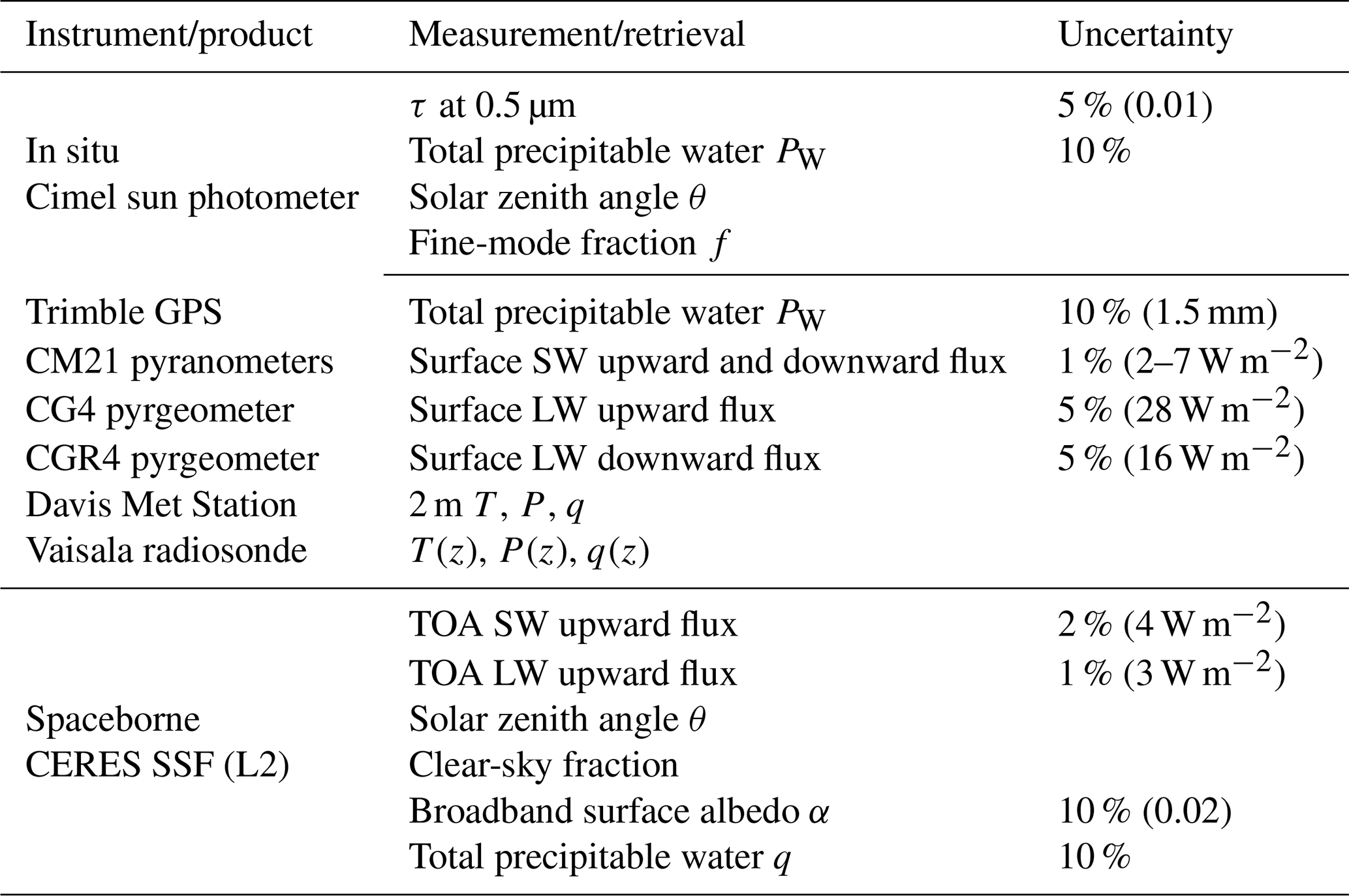
Here we describe the in situ and satellite-based datasets used in this study. A listing of the instruments, products, measurements, and retrievals, as well as their uncertainties, is in Table 1.
2.1 Field site description, instruments, and measurements
The in situ measurements used in this study were generated over the 2020–2022 time period at a field site in southeastern California (33.17° N, 115.86° W; Fig. 1). The field site lies within the Salton Basin, which is a northwest–southeast-oriented rift valley that is bounded to the west, north, and south by the Peninsular, Little San Bernadino, and Orocoppio and Chocolate Mountains, respectively. At the sub-sea-level center of the basin is the terminal Salton Sea, a large and shallow ephemeral lake. The region typically receives less than 100 mm of precipitation each year (Stephen and Gorsline, 1975; NCEI, 2023). During the summer daytime surface temperatures often reach values greater than 38 °C, while winter temperatures are moderately cool and can fall below freezing at night (Ives, 1949; Imperial County Air Pollution Control District, 2018). The morphology of the area includes alluvial fans, sand and sand dunes, dry washes, a paleo-lake bed, and rock and vegetated surfaces (Imperial Irrigation District, 2016).
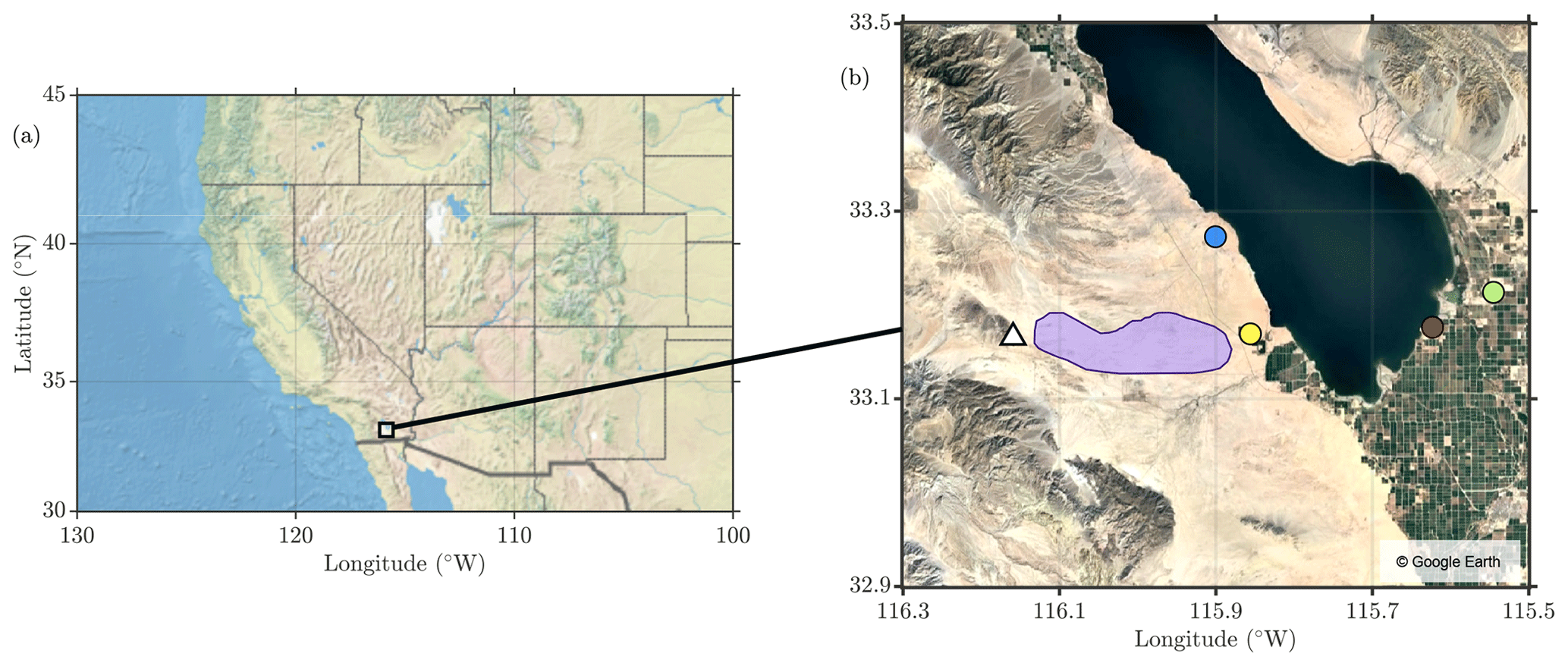
Figure 1Map of the region of interest. Shown is (a) a map indicating the location of the Salton Basin and its relation to the western United States and (b) key locations surrounding the Salton Sea. The region enclosed by the purple polygon in (b) was used to generate the surface soil mineralogy for the radiative transfer simulations. Also shown in (b) are the locations of the field site (yellow circle), Roundshot camera (white triangle), and the Salton City, Naval Test Base, Sonny Bono, and Niland–English Road TEOM sites (blue, yellow, red, and green circles, respectively). The map shown in (a) is created using Natural Earth via MATLAB, and the map in (b) is from Google Earth, retrieved 26 August 2023.
In situ measurements presented here were collected over the 2020–2022 time period at a field site that lies approximately 2.5 km west of the Salton Sea's current western shoreline. The site is immediately east of the Anza Desert and is at the northern and southern edges of the Imperial Valley and Coachella Valley, respectively (Fig. 1b). Measurements from the site acquired during dust storms have been used to elucidate their meteorological aspects (Evan et al., 2022b, 2023). A photo of the field site instrumentation is in Fig. 2.
2.1.1 Solar and infrared radiometers
We obtained surface LW upward and downward fluxes from Kipp & Zonen CG4 and CGR4 pyrgeometers (1A in Fig. 2). These radiometers measure broadband LW fluxes in the 4.5–42 µm range, are outfitted with Pt-100 thermistors to measure instrument body temperature, and have previously reported relative uncertainties of approximately ±3 % (Ramana and Ramanathan, 2006). Longwave fluxes are acquired every second and then averaged over 1 min intervals. We obtained surface SW upward and downward fluxes from two Kipp & Zonen CM21 pyranometers (2A in Fig. 2). These radiometers measure broadband SW fluxes in the 0.3–2.8 µm range and exhibit small cosine offsets with a typical maximum relative error of 3 % at high solar zenith angle (Zonen, 2004; Ramana and Ramanathan, 2006). Shortwave fluxes are also acquired every second and averaged over 1 min intervals.
A detailed description of the radiometer calibration is in Appendix B. One pyranometer and one pyrogeometer were factory-calibrated in July 2018 and then February 2023, and the pyranometer and pyrogeometer calibration coefficients for these two dates differed by less than 2 % and 3 %, respectively. We then cross-calibrated the other pyranometer and pyrogeometer during four distinct time periods occurring in 2018, 2021, 2022, and 2023. To do so we placed the instruments side by side for time periods ranging from 1–3 weeks and then used linear least-squares regression to identify the slope of the best-fit line relating the measured voltages, forcing the intercept through zero. For these four time periods the pyranometer and pyrgeometer cross-calibration coefficients differed by up to 2 % and 3 %, respectively. The factory and cross-calibration coefficients were then applied to the measured voltages by interpolating their values in time in order to obtain the final LW and SW fluxes. Since the uncertainty in the cross-calibration coefficients was <0.3 %, we assume factory calibration uncertainties of 1 % for the pyranometer and 5 % for the pyrogeometer as the uncertainty in the radiometer SW and LW fluxes, respectively (Table 1).
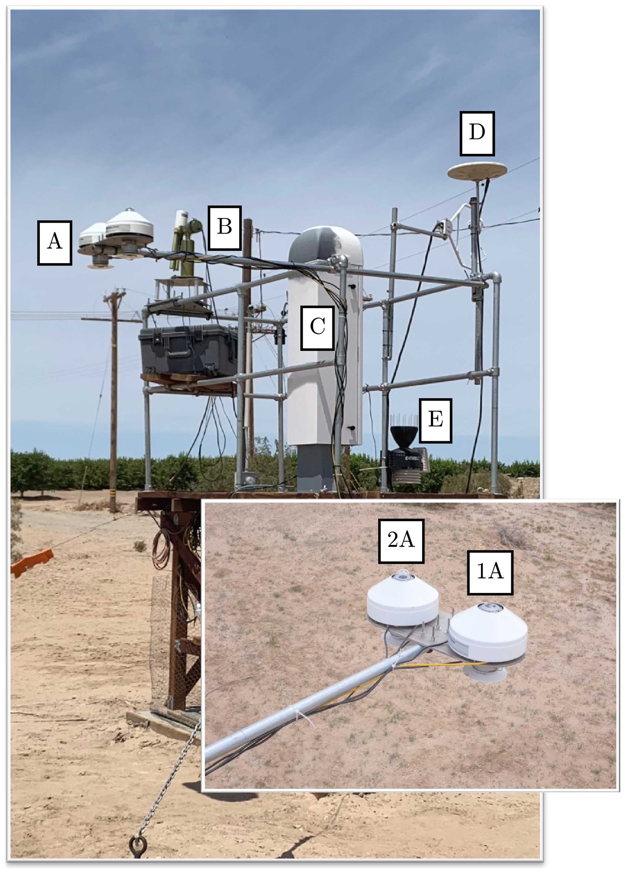
Figure 2Instrumentation at the field site. Shown are radiometers (A), sun photometer (B), ceilometer (C), GPS antennae (D), and meteorology station (E). The inset panel indicates the upward- and downward-looking pyrgeometers (1A) and the upward- and downward-looking pyranometers (2A). Radiometer (1A and 2A) image credit: Scott Polach.
2.1.2 GPS
We obtained hourly values of total precipitable water PW retrieved from a Zephyr Geodetic 2 Antenna and Trimble NetR9 GPS receiver (D in Fig. 2), which were processed by SuomiNet (Ware et al., 2000). The relative uncertainty in PW from the GPS is approximately 10 % (Wang et al., 2007; Bevis et al., 1994).
2.1.3 Sun photometer
At the field site is a NASA Aerosol Robotic Network (AERONET) Cimel sun photometer (B in Fig. 2). The Cimel measures sun-collimated direct-beam irradiance and directional sky radiance at eight spectral bands centered on 1020, 870, 675, 440, 936, 500, 380, and 340 nm (Holben et al., 1998). Direct solar irradiance measurements are made at 5 min intervals. We obtained data from the AERONET level 1.5 products processed by the version 3 AERONET algorithm, which provides fully automatic cloud screening and instrument anomaly quality controls in near-real time (Giles et al., 2019). We included dusty observations that were erroneously classified as cloud-contaminated using the restoring algorithm described in Evan et al. (2022c). AERONET-retrieved aerosol optical depth τ has a reported absolute uncertainty of 0.01 (an approximate 5 % relative error for the field site), and PW has a reported relative uncertainty of approximately 10 % (Holben et al., 1998).
Since PW from the GPS was not available at all study times we utilized PW retrievals from AERONET for this analysis. We calibrated the AERONET PW based on a comparison with retrievals from GPS. Over the 2020–2022 time period we identified more than 6000 simultaneous retrievals of PW from these two instruments, which were correlated at an r value of 0.99 (p value <0.01, Fig. 3). We calibrated the AERONET PW against that from the GPS to account for a relative negative bias in AERONET PW by multiplying the AERONET values by 1.43, which was the slope of the best-fit line from a linear regression of the GPS PW on the AERONET PW, forcing the line through the origin (red line, Fig. 3). The resulting root mean square error in the AERONET PW is 0.15 cm (10 % relative uncertainty).
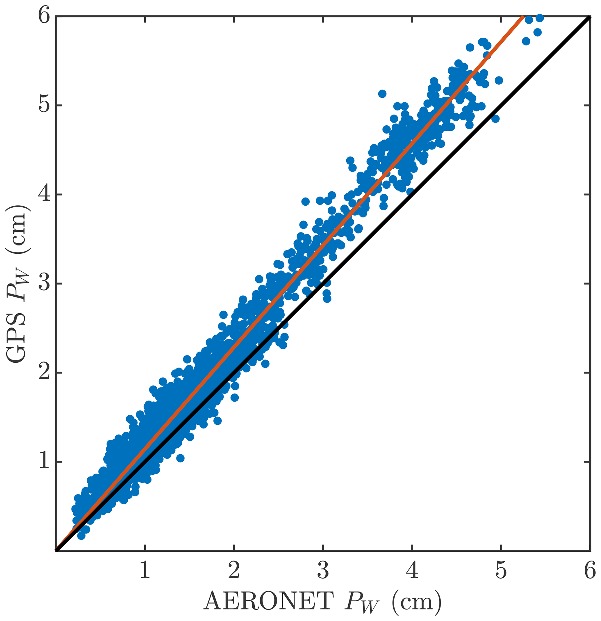
Figure 3A scatter plot of GPS (vertical axis) and AERONET (horizontal axis) retrievals of PW (blue) made at the field site, the 1-to-1 line (black), and the linear least-squares regression line, forced through the origin (red).
2.1.4 Ceilometer
At the field site is a CL51 Vaisala ceilometer (C in Fig. 2), which is a single-lens lidar system that measures attenuated backscatter at a nominal wavelength of 910 nm from the surface to 15 km. The ceilometer generates range-corrected backscatter profiles with temporal and vertical resolutions of 36 s and 10 m, respectively. The Vaisala processing software for the CL51 measurements, BLView, identifies clouds based on the vertical gradient of backscatter profiles. Ceilometers have been used to retrieve the vertical profile of aerosols in the lower atmosphere (Jin et al., 2015; Marcos et al., 2018; Münkel et al., 2007), and the BLView software also retrieves vertical profiles of extinction for the clear-sky atmosphere below heights of 5 km above ground level (a.g.l.). Although details regarding the retrieval process used in BLView are not publicly available, it is possible to approximately reproduce the extinction profile retrievals using typical methods (Fernald, 1984). The CL51 extinction profiles used here were calibrated to equivalent 500 nm values using the simultaneous retrievals of aerosol optical depth from the AERONET site (Evan et al., 2022c) such that the AERONET- and CL51-retrieved optical depths are identical.
To guard against cloud contamination in our analysis and results we identified all times when the ceilometer's proprietary software identified a cloud overhead. Since the ceilometer software's cloud detection algorithm often misidentifies thick dust plumes as clouds, we discarded all detected clouds with a base height less than or equal to 2 km a.g.l. (Evan et al., 2022c). We then assumed that the sky is at least partially cloudy if a cloud was detected within a 30 min window by the ceilometer (Wagner and Kleiss, 2016), and thus did not include these data in our analysis.
2.1.5 Meteorological measurements
Surface meteorology. A Vantage Pro2 Davis Met Station is also located at the site (E in Fig. 2) and provides measurements of pressure P, temperature T, specific humidity q, and zonal (u) and horizontal (v) wind speed at a height of 2 m, which are logged at a 1 min resolution. These data are separately processed and available through MesoWest at a nominal resolution of 15 min (Horel et al., 2002).
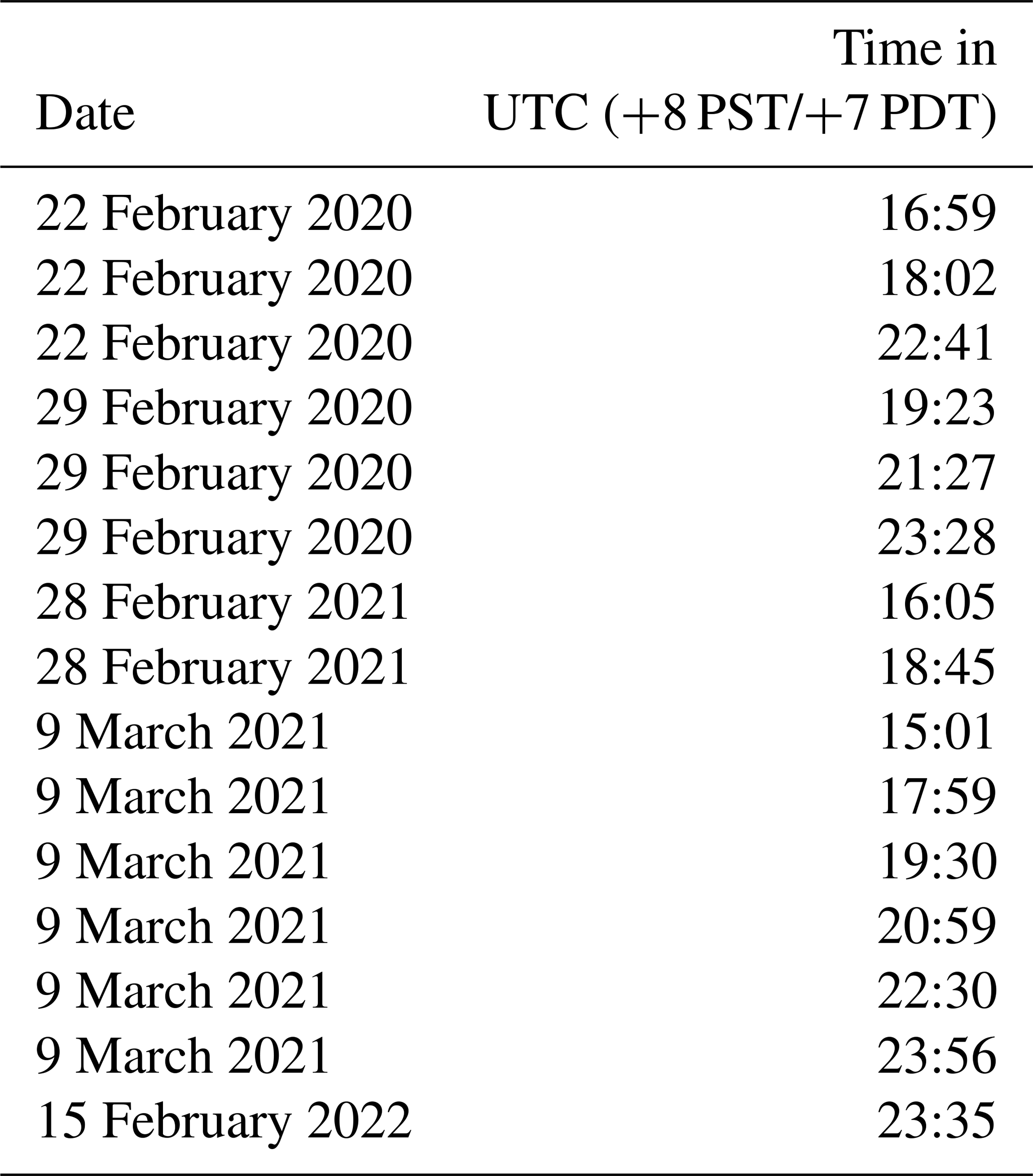
Radiosondes. We obtained vertical profiles of temperature T(z), pressure P(z), and specific humidity q(z) from 15 radiosondes launched at the field site during the 2020–2022 time period using a Vaisala sounding system (dates and times listed in Table A1). Since these soundings typically extend to heights of 20–25 km and in order to conduct the radiative transfer simulations, we extended these profiles to heights of 32 km using radiosondes from the San Diego sounding station (NKX) and then from 32 to 95 km using a standard midlatitude summer atmospheric profile (Anderson et al., 1986).
Table 1Instrumentation and measurements or retrievals used in this study either at the field site (top) or from spaceborne platforms (bottom). Uncertainties are indicated for measurements and retrievals that are used to calculate the dust direct radiative effect and forcing efficiency.
2.2 Satellite data
We collected observations of the TOA SW upward flux and outgoing longwave radiation (OLR), as well as estimates of the broadband SW surface albedo α from the Clouds and Earth's Radiant Energy System (CERES) Single Scanner Footprint (SSF) level 2 data product (Loeb et al., 2016; Su et al., 2015a, b). CERES is a spaceborne instrument that measures TOA radiance in the SW (0.2–5 µm), window (8–12 µm), and total (0.2–100 µm) spectral intervals at a spatial resolution of approximately 20–25 km. Longwave radiance is estimated by taking the difference between the total and SW radiances. Instantaneous CERES SSF measurements are collected along-scan of the CERES footprint as it traverses the Earth's surface.
We used daytime CERES SSF level 2 data collected from the NASA Aqua, NASA Terra, National Oceanic and Atmospheric (NOAA) Suomi National Polar-orbiting Partnership (NPP), and NOAA-20 sun-synchronous satellites. The SSF data corresponding to the CERES instruments flying on the NASA satellites include retrievals and products from the Moderate Resolution Imaging Spectroradiometer (MODIS) instruments on those platforms, while those flying on the NOAA satellites include that from Visible Infrared Imaging Radiometer Suite (VIIRS) instruments. This data product also includes footprint-averaged deep blue aerosol optical depth retrievals (Hsu et al., 2013), surface albedo (Rutan et al., 2009), and PW from the Goddard Earth Observing System Model version 5.4.1 reanalysis (Rienecker et al., 2008).
In order to obtain CERES data representative of the conditions over the field site, we limited our analysis to footprints with a nadir center point within approximately 25 km of the field site (Fig. 4). We obtained clear-sky fraction from the CERES level 2 clear/layer/overlap condition percent coverage parameter (Wielicki et al., 1996) and further limited our analysis to satellite footprints with clear-sky fraction ≥95 %. We only utilized CERES data if the measurement was generated within 30 min of an AERONET measurement. These constraints resulted in 1639 CERES level 2 SSF products over the 2020–2022 time period that were considered for our analysis (Fig. 4).
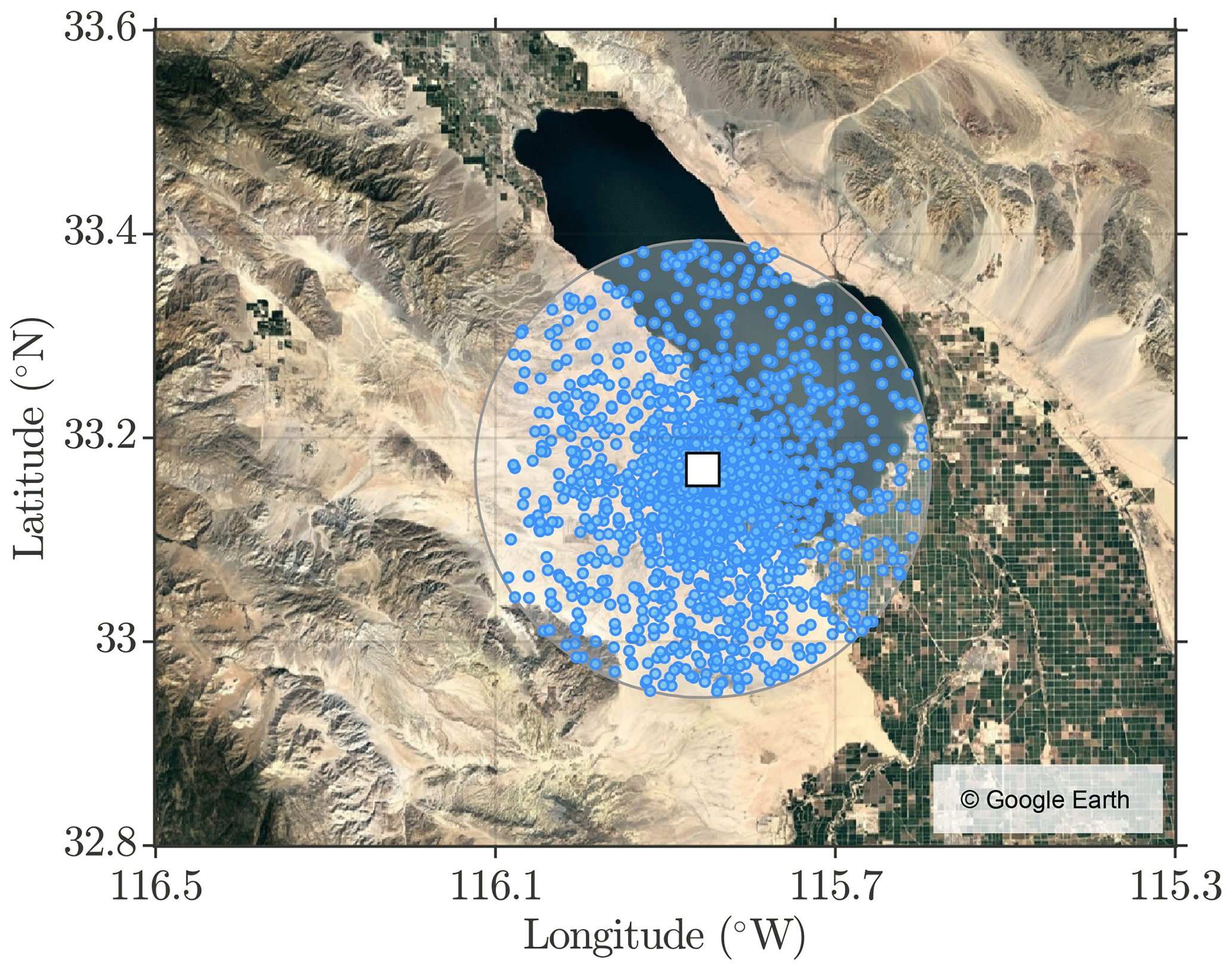
Figure 4Nadir-looking points of the CERES SSF level 2 data considered in this study. Shown are CERES SSF footprints (closed blue circles) with centers within approximately 25 km of the field site (white square) during daytime and both dusty and non-dusty conditions. CERES SSF footprints shown here are selected when the CERES clear-sky fraction is greater than or equal to 95 % (i.e., cloud-free). The map shown is from Google Earth, retrieved on 26 August 2023.
2.3 Other datasets
We obtained vertical profiles of temperature and geopotential height over the field site from the Japan Meteorological Agency 55-year reanalysis (JRA-55), which are available at 6-hourly time increments at a 0.5° spatial resolution (Japan Meteorological Agency, Japan, 2013). The JRA-55 reanalysis data were included in this study because this dataset was the only reanalysis available from the National Center of Atmospheric Research (NCAR) with a 4D-Var data assimilation scheme through 2019 to 2022. We used measurements of concentrations of particulate matter with diameters under 10 µm (PM10) from tapered-element oscillating microbalance (TEOM) instruments at several monitoring sites located around the periphery of the Salton Sea (filled circles in Fig. 1). These data are only available at a 1 h temporal resolution from the California Air Resources Board. Lastly, we obtained images of dust storms from a 360° Roundshot web camera that is maintained by the Imperial Irrigation District. The camera lies at an elevation of 300 m and is 28 km west of the field site (filled triangle in Fig. 1). Roundshot images are available at approximate 10 min intervals during daytime hours via https://iid.roundshot.com/anza-borrego/#/ (last access: 7 August 2023) and are typically unavailable during July–September.
2.4 Identifying dust storms
Here we describe the method employed to identify dust storms passing over the field site during the daytime hours. Firstly, potential dust storms were manually and subjectively identified via visual inspection of backscatter profiles from the site ceilometer for the 2020–2022 time period. We typically selected times of potential dust when there was a strong (>3 a.u.) and persistent (approximately >30 min) backscatter signal near the surface that extended to heights of 500 m to 3 km, which is typical of dust storms over the region (e.g., Evan et al., 2022b, 2023). For example, ceilometer profiles for a 24 h time period beginning at 02:00 UTC on 22 April 2022 indicate the likely presence of dust during this time period and would thus be flagged as a potential dust storm for further analysis (Fig. 5a). From these potential storms, we assumed individual AERONET measurements are made during dusty scenes if the AERONET fine-mode fraction is <0.5 (Evan et al., 2022c) and if PM10 from one of the nearby TEOM stations is ≥50 µg m−3 within an hour of the observation (Hoffmann et al., 2008). We note that if fine-mode fraction data were missing we defined a 440–870 nm Ångström exponent threshold of ≤0.25 as a substitute, which is based on a comparison of fine-mode fraction and Ångström exponent data for other confirmed dust cases (not shown). These additional criteria limited our analysis to clear-sky conditions and daytime data (e.g., mauve boxes in Fig. 5a).
When possible, we additionally confirmed the presence of dust in the region via visual inspection of Roundshot camera imagery (location in Fig. 1), specifically identifying dust in the eastward-looking – towards the field site – direction (e.g., Fig. 5b). Since we have observed days when there was dust at the surface but smoke from regional biomass burning events suspended above the dust layer, we excluded dust events if there was an elevated aerosol layer apparent in the ceilometer backscatter profiles or if inspection of visible satellite imagery for these events showed smoke in the region.
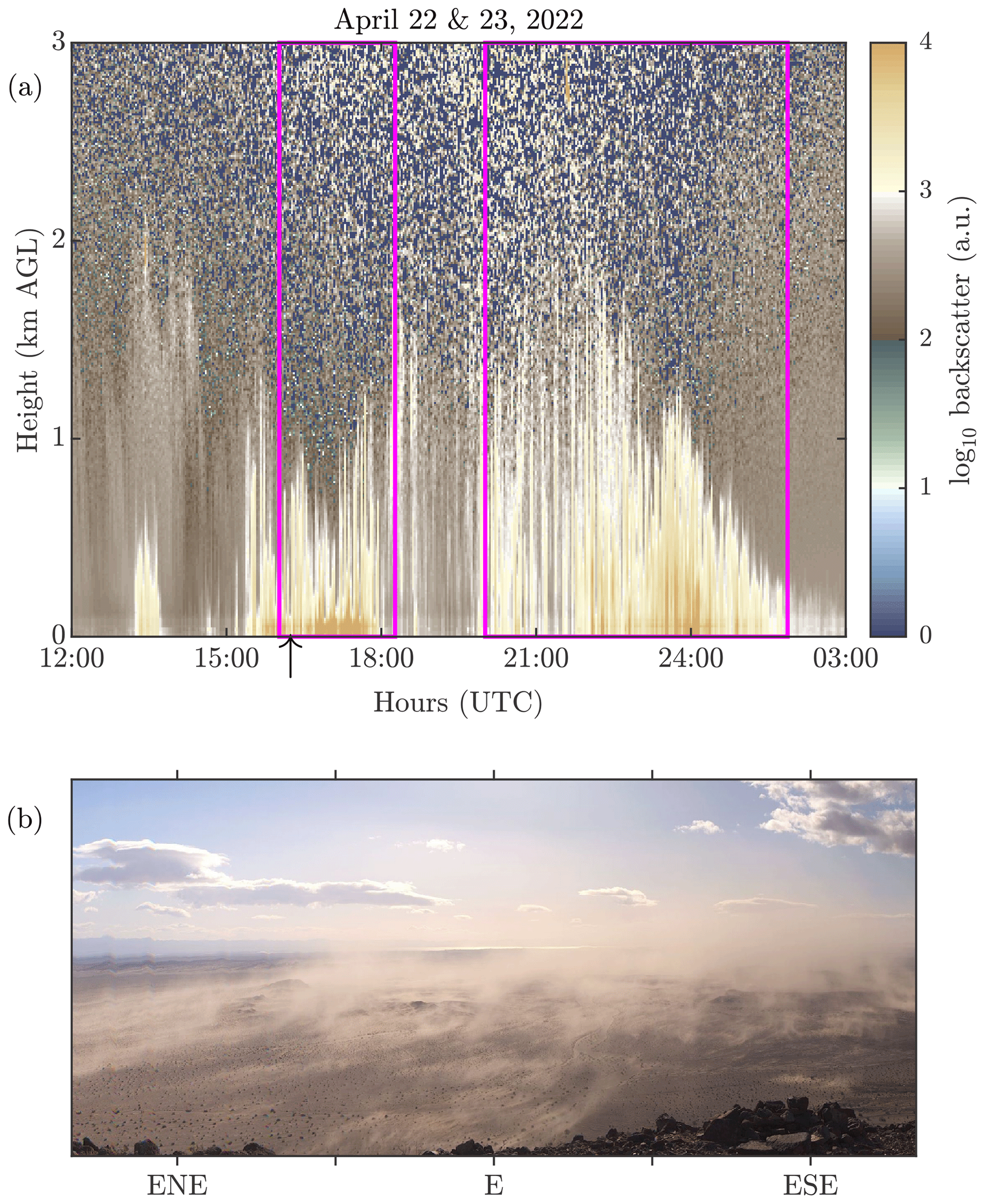
Figure 5(a) Example of a backscatter profile generated from the site ceilometer during a dust storm on 22 and 23 April 2022. Times enclosed by the magenta lines were identified as being dusty after analysis of additional data sources. (b) Eastward-looking Roundshot image captured at 16:00 UTC on this date – black arrow on the horizontal axis in panel (a). The Roundshot image in (b) can be obtained via https://iid.roundshot.com/anza-borrego/#/ (last access: 22 September 2022).
This method to identify dust storms resulted in the identification of approximately 2215 AERONET observations during which there was a dust storm over the field site during 2020–2022. This number was reduced to approximately 1964 when we also limited the data to times when SW and LW radiometer measurements were available from the field site. We note that there were other dust storms over the site that were not included in this analysis because of intermittent issues with instrumentation (e.g., loss of site power, contamination of instrument optics) or because dust storms in the region are oftentimes accompanied by cloud cover (e.g., Evan et al., 2023); as such, this estimate does not represent a complete account of all dust storms in the area. Of the 1639 satellite observations that were collocated with the field site, only 43 were made within 30 min of an identified clear-sky dust event and were thus used in our analysis.
Lastly, most dust events over the field site are associated with strong (e.g., >10 m s−1 10 m wind speeds) westerly winds (Evan, 2019; Evan et al., 2023). For example, for the 22 April 2022 case the 10 m wind speeds and gust measured at the site were westerly and typically 10 and 20 m s−1, respectively (not shown). Furthermore, these strong westerly winds typically originate at altitudes above the mountain ridges that lie to the west of the field site, which have heights of 2–3 km, before they descend along the lee-side mountain slopes, passing over generally uninhabited landscapes. As such, and given the fine-mode fraction threshold test required to classify an observation as being acquired during a dust storm, we assume that during dust storms the aerosols over the site are dominated by mineral species and that other aerosols constitute a negligible fraction of the total burden.
Based on our dust identification scheme, the average τ at the field site and during dust storms is 0.18, with a standard deviation of 0.11 and a maximum retrieved value of 2.0.
2.5 Surface soil mineralogy
In order to calculate the complex refractive index of dust over the field site we estimated the average soil mineralogy over the dust-emitting regions that are typically upwind (i.e., to the west) of the field site (purple polygon in Fig. 1), which are identified from analysis of satellite imagery of dust outbreaks and eye-witness accounts. Surface soil mineralogy is from the Airborne Visible/Infrared Imaging Spectrometer - Classic (AVIRIS-C), which is a passive imaging spectrometer that operates in the 0.41–2.45 µm wavelength range and is designed to operate aboard NASA's Earth Resources 2 aircraft (Chrien et al., 1990). The AVIRIS-C measurements used here were collected over the region in 2018, and from these data the approximate mineral abundance for the following nine minerals are retrieved: calcite, chlorite, dolomite, goethite, gypsum, hematite, illite, kaolinite, and montmorillonite (Thompson et al., 2020). Also retrieved from AVIRIS-C are estimates of the fractional cover of major land surface types, from which fractional bare soil cover was used here.
3.1 Radiative transfer model
In this study we utilize the SW Rapid Radiative Transfer Model (RRTM) version 2.5 (Atmospheric and Environmental Research, 2004) and LW RRTM version 3.3 (Atmospheric and Environmental Research, 2010) from Atmospheric and Environmental Research (AER), Inc. (Mlawer et al., 1997; Mlawer and Clough, 1997, 1998). This version of RRTM is a band transmission model that evaluates radiative transfer at 14 spectral bands ranging from 0.2–12.2 µm and 16 spectral bands from 3.1–1000 µm (Iacono et al., 2008; Clough et al., 2005). The model uses the correlated-k method to treat gaseous absorption. In the SW code, the correlated-k method is applied to the solar source function, which derives the incoming solar flux at the TOA (Mlawer and Clough, 1998). We use eight streams in the Discrete Ordinate Radiative Transfer (DISORT) to solve radiative transfer for multiple scattering in both the SW and LW spectrum (Iacono et al., 2008). Each SW band uses a present-day solar source function and a spectrally constant broadband surface SW albedo α. Correspondingly each LW band uses a constant broadband LW α of 0.01. We assume a CO2 mixing ratio of 417 ppm, which is the approximate average atmospheric CO2 concentration measured at Mauna Loa in middle to late 2021. Other gases that are included in the model are water vapor, nitrogen, ozone, nitrous oxide, methane, oxygen, carbon monoxide, and the halocarbons CCL4, CFC112, CFC12, and CFC222. The model assumes Lambertian reflection at the surface. RRTM SW has been extensively validated against the Line-by-line Radiative Transfer Model (LBLRTM), an accurate line-by-line model that is continuously validated against observations; the coefficients used in the correlated-k method are developed via LBLRTM. In the SW, RRTM is in agreement within 1.5 W m−2 with LBLRTM (Clough et al., 2005).
For the RRTM simulations, we estimate the dust complex refractive index (CRI) using the surface soil mineralogy described in Sect. 2.5 and the methods described in Walkowiak (2022). Briefly, we first average the mineral abundances over the polygon shown in Fig. 1, weighing each 20 m horizontal resolution AVIRIS-C grid cell by its corresponding bare soil fraction. The retrieved AVIRIS-C soil mineralogy (and uncertainty range) is 7(0–21) % calcite, 3(0–9) % kaolinite, 2(0–5) % goethite, 2(0–8) % montmorillonite, 0.5(0–2) % hematite, and 0.5(0–3) % illite, with the abundances of chlorite, dolomite, and gypsum being <0.01 % (Fig. 6). We assume that the remaining fractional soil abundance is composed of silicate minerals (quartz and feldspar) whose fractional abundance is not retrieved by AVIRIS-C given their relatively flat spectral variation in the visible, with the concentration of the silicates being 85(52–100) %.
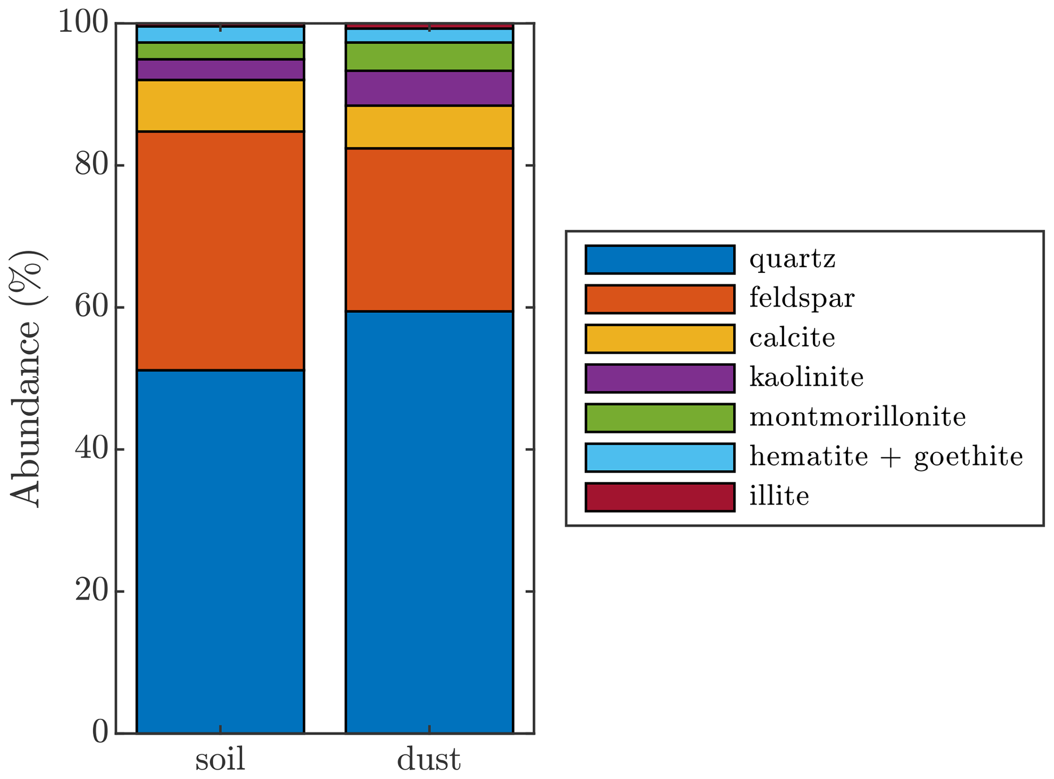
Figure 6Mineral abundances of the surface soil and dust based on AVIRIS-C-retrieved mineral abundance averaged over the polygon in Fig. 1.
We apply the methods described in Scanza et al. (2015) to generate a dust CRI from a surface soil mineralogy. Firstly, we partition the surface mineralogy into clay and silt sizes, assuming that the fractional surface soil abundance of a mineral m is
where mc and ms are the soil mineral abundances in the clay and silt sizes, respectively, and fc and fs are the fractional abundances of clay and silt in the soil, respectively, which are calculated from the soil probability size distribution in Kok (2011). We define the ratio of mineral abundance rm in the clay and silt size ranges as , which allows us to express ms and mc, via Eq. (1), as
and
We obtain rm for each AVIRIS-C mineral via the clay and silt fractional abundances for the Calcaric Fluvisol soil type in Claquin et al. (1999) and then estimate the fractional contribution of each to the soil clay and silt sizes via Eqs. (2) and (3). Assuming that the unclassified abundances in the clay and silt sizes are comprised of quartz and feldspar, we proportionally assign their fractions within each soil size class via their relative abundances for the same soil type (Claquin et al., 1999). For this case, the total soil abundances of quartz and feldspar are 51 % and 34 %, respectively (Fig. 6). We obtain similar results when repeating this process but using the Luvic Yermosol soil type abundances from Claquin et al. (1999) and using the reported abundances for these two soil types from Journet et al. (2014, not shown). We then utilize the dust size distribution in Meng et al. (2022) to estimate a corresponding dust mineralogy, although we obtained similar results when using that from Kok (2011).
We utilize a modified version of methods in Song et al. (2023) to estimate a resulting CRI from this dust mineralogy. To do so, we generate volume-averaged dielectric constants for the clay minerals (illite, kaolinite, montmorillonite) and silicates (quartz, feldspar), since these clays and the silicates exhibit similar complex indices of refraction. For the iron oxides, we assume that goethite has the same index of refraction as hematite since there is not a goethite index of refraction that spans the shortwave and longwave part of the spectrum (Scanza et al., 2015). Since the fractional abundance of dolomite is approximately zero, the carbonate refractive index is just that of calcite. Gypsum is not considered since the soil abundance of this mineral is also negligible. The complex indices of refraction for the clay, silicate, iron oxide, and carbonate minerals are in Fig. C1. We calculate an effective dielectric constant for the aerosol by averaging those for the clay, silicate, carbonate, and iron oxide minerals via the Maxwell–Garnett mixing rule, assuming the mineral group with the greatest aerosol abundance (the silicates) is the parent material, and then adding the remaining mineral groups as inclusions in order of decreasing volume fraction. The complex index of refraction is then obtained from the resulting effective dielectric value (black lines, Fig. 7). We note that we obtain a qualitatively similar CRI when using the Bruggeman mixing method, consistent with Song et al. (2023).
To account for uncertainty in the soil mineralogy retrievals we repeated the above calculation of the complex index of refraction using a Monte Carlo method to sample from the distribution of soil mineralogy values, which was determined using the reported AVIRIS-C uncertainties for each mineral retrieval. The 1σ uncertainties in the complex refractive index are represented by the gray shaded regions in Fig. 7.
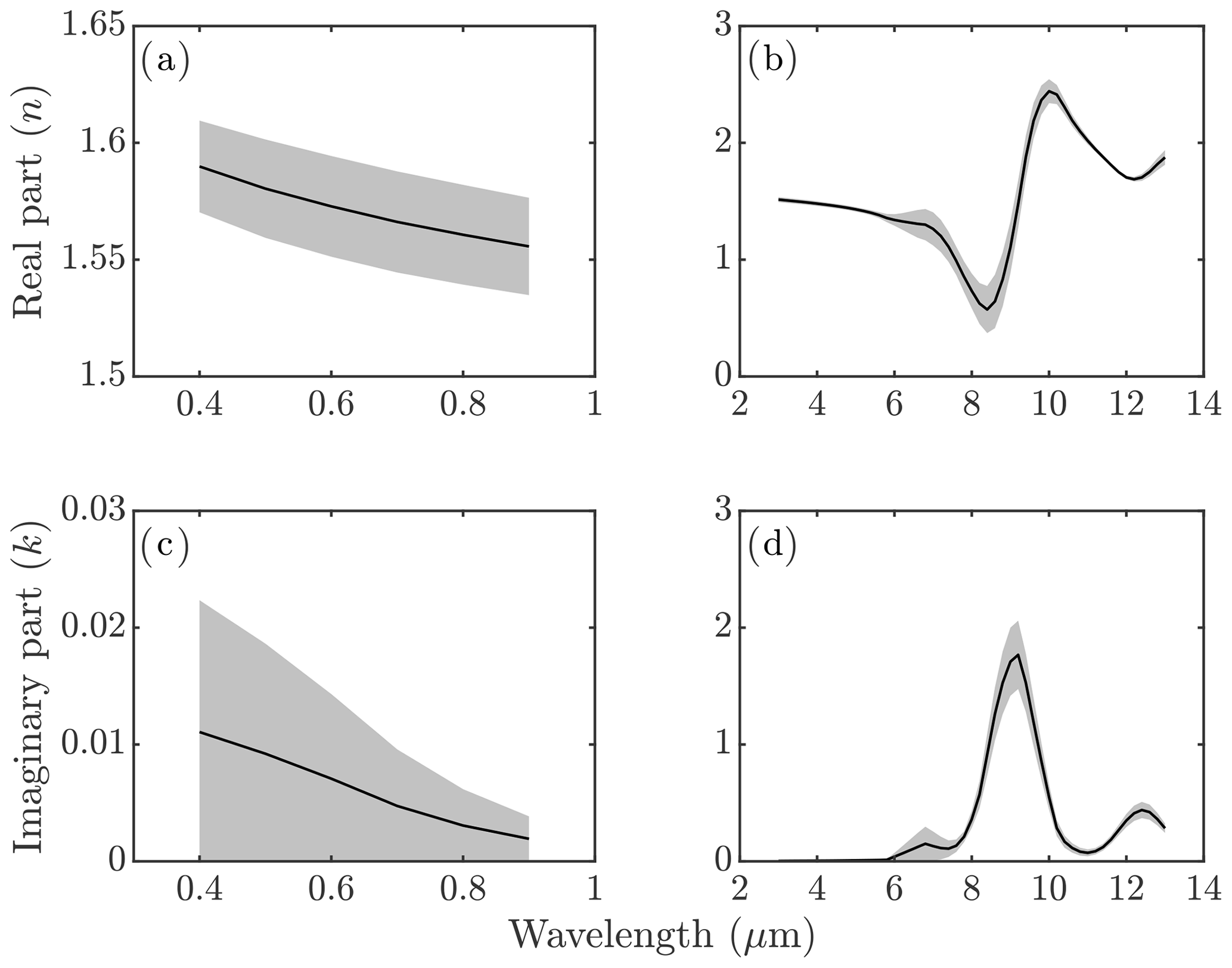
Figure 7Real part (n) of the complex refractive index calculated from the AVIRIS-C surface soil mineralogy in the (a) solar and (b) infrared, as well as the imaginary (k) part of the index in the (c) solar and (d) infrared.
In the solar part of the spectrum we obtain a slightly decreasing real part of the refractive index n (Fig. 7a) and a pronounced decrease in the imaginary part k (Fig. 7c) with increasing wavelength. The absorption in the visible is due to the abundance of iron oxide (Fig. C1), which has a large imaginary index of refraction at these wavelengths (e.g., Doner et al., 2019). Consequently, the uncertainty in the refractive index in the solar part of the spectrum is mainly due to that of the iron oxide content; assuming no uncertainty in the goethite and hematite concentrations resulted in refractive indices with almost no uncertainty in k and an order magnitude reduction in uncertainty in n (not shown). Since the reported AVIRIS uncertainty in the iron oxides included a fractional abundance of zero, the resulting uncertainty in k is approximately 100 %. The spectral variations in n and k in the shortwave are similar to results obtained by Di Biagio et al. (2019).
In the longwave part of the spectrum the minimum in n at approximately 8.5 µm and the peak at 10 µm (Fig. 7b), as well as the peak in k near 9 µm (Fig. 7d), reflect similar spectral features in the silicates and clay minerals (Fig. C1). Consequently, the longwave uncertainty in the index of refraction is mainly due to uncertainty in the fractional abundance of quartz and feldspar, which was confirmed by setting those uncertainties to zero in the calculation of the refractive indices (not shown). We note that the longwave refractive indices in Fig. 7b and d are qualitatively similar in spectral structure to those estimated for North American dust by Di Biagio et al. (2017), although here the magnitudes of n and k are larger by factors of approximately 1.5 and 3. These relatively large values of n and k in the longwave are due to the relatively high abundance of quartz and feldspar estimated from the AVIRIS retrievals (Fig. 6).
3.1.1 Dust single-scattering properties
We obtain dust single-scattering properties from the Texas A&M University dust 2020 (TAMUdust2020) version 1.1.0 database of optical properties of irregular aerosol particles (Saito et al., 2021a). This database generates single-scattering properties of randomly oriented and irregularly shaped dust particles given a CRI and degree of asphericity by considering ensembles of at least 20 irregular hexahedral particles. We use the previously described dust CRI (Fig. 7) and use the default model dust asphericity, which is consistent with the global mean dust particle aspect ratio reported in Huang et al. (2020).
We assume that the dust particle size distribution changes with height via a power-law dependency having a particle-size-dependent exponent of (Shao, 2008), where κ is the von Kármán constant, α is a diffusivity scaling parameter, u* is the friction velocity, which we assume is 0.4 based on measurements made with a 3-D sonic anemometer at the field site during dust storms (not shown), and wt is the size-dependent particle terminal velocity, which is proportional to the square of the particle diameter. We then scale the emitted dust size distribution in Meng et al. (2022) with height accordingly and calculate a dust layer average using the mean vertical profile of dust from the site ceilometer, which extends to 1.7 km a.g.l. We then use this layer-mean dust size distribution to calculate the spectrally resolved single-scattering properties from the TAMUdust2020 model output via standard methods (e.g., Seinfeld and Pandis, 2016).
It is not practical to conduct simulations with the TAMUdust2020 model for each of the dust complex refractive indices generated from the Monte Carlo simulations. However, since the main source of uncertainty in Fig. 7 is the concentration of iron oxides (i.e., k in Fig. 7c), we conducted two additional simulations with TAMUdust2020 using the imaginary indices of refraction corresponding to the ±1σ uncertainty in k in the solar part of the spectrum (i.e., the uppermost and lowermost shaded regions in Fig. 7c, d). We repeated this exercise by also varying n according to the uncertainty shown in Fig. 7a and b, obtaining similar results, which underscores that the uncertainty in the iron oxide content of dust dominates the uncertainty in the resulting single-scattering properties.
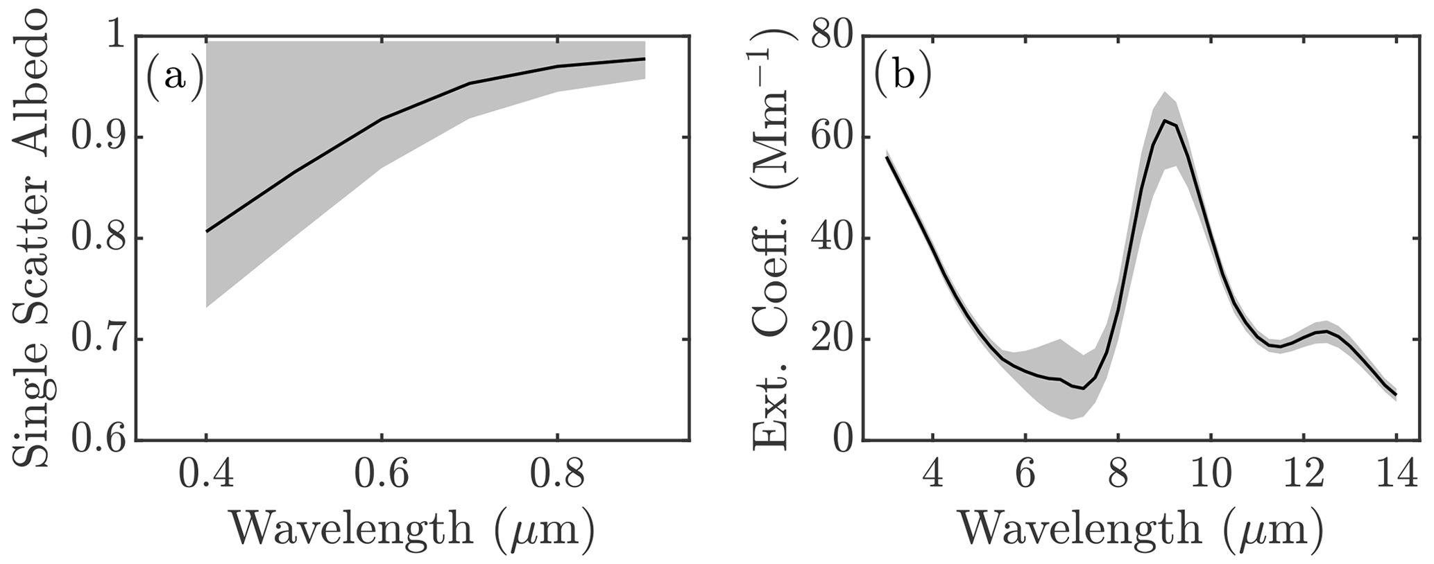
The single-scattering properties generated from the TAMUdust2020 output exhibit characteristics typical of dust (e.g., Highwood and Ryder, 2014). In the shortwave we obtain an increasing single-scattering albedo with increasing wavelength, but the uncertainty is large, with the single-scattering albedo having a possible value of 1, corresponding to no solar absorption (Fig. 8a). Spectral peaks in the longwave extinction coefficient (Fig. 8b) that correspond to those in the absorption spectra (Fig. 7d), with uncertainty in the 6–10 µm range, are also similar to that of the complex refractive index. These characteristics of the single-scattering albedo and extinction coefficient are similar to those presented in studies of dust single-scattering properties (Di Biagio et al., 2017; Di Biagio et al., 2019).
3.1.2 Radiative transfer model simulations
We conduct RRTM simulations corresponding to the AERONET observations made during the identified dust storms. For the model simulations we define 107 radiative transfer model levels and specify the vertical profiles of pressure, temperature, and water vapor from reanalysis (Sect. 2.3). We calibrated the reanalysis water vapor profiles so that the resulting total precipitable water Pw equaled that retrieved from AERONET. For each simulation we used the broadband SW albedo given by the site pyranometers, which ranged from 0.23–0.38 (not shown). We use a constant broadband LW surface albedo of 0.01, which is an average LW surface emissivity retrieved from the CERES observations used in the study (Fig. 4). We estimate the surface temperature for each simulation using the measured upwelling LW flux at the site and the average CERES surface emissivity. We specify the vertical distribution of dust extinction at 500 nm via the calibrated retrievals from the ceilometer. We conduct a separate set of simulations with aerosol optical depth set to zero in order to quantify the model dust radiative forcing. We conduct two additional sets of simulations with RRTM using the upper and lower bounds of the dust single-scattering albedo (Fig. 8a) to estimate the uncertainty in the calculated fluxes associated with uncertainty in the dust iron oxide content.
We conduct a third set of RRTM simulations corresponding to clear-sky and daytime scenes during which we obtained vertical profiles of pressure, temperature, and moisture from 15 radiosondes launched at the site during the 2020–2022 time period and on days when dust storms occurred (radiosonde launch times are in Table A1). These simulations were carried out in a manner identical to those described above except that the model was forced with the sounding profiles rather than reanalysis output.
3.1.3 Radiative transfer model comparison to observations
We assess the uncertainty in simulated SW and LW fluxes via comparison to observations. We characterize the model uncertainty as the bias-corrected root mean square error (RMSE) between modeled and measured net fluxes, since biases in the modeled fluxes do not affect our calculations of the direct radiative effect or forcing efficiency. We begin by evaluating the modeled surface fluxes for the simulations using the radiosonde measurements, which include 13 cases for the SW flux comparisons and 15 cases for the LW flux comparison (for two radiosondes the pyranometers were not operational). There was a −10 and −8 W m−2 bias (2 % and 5 % relative bias) in the modeled net surface SW and LW fluxes, respectively. A comparison of the bias-corrected net SW (Fig. 9a) and LW (Fig. 9b) surface fluxes indicates that the model reasonably reproduces the observed fluxes; the bias-corrected SW and LW RMSE is 6 W m−2 (1 % relative error) and 4 W m−2 (2 % relative error), respectively. We note that the differences between the modeled and measured fluxes were not correlated with aerosol optical depth τ, although the small sample size precludes definitive assessment of the impact of dust on model uncertainty. Here we do not compare modeled and satellite-observed TOA fluxes since only two clear-sky satellite measurements were available during the radiosonde launches.
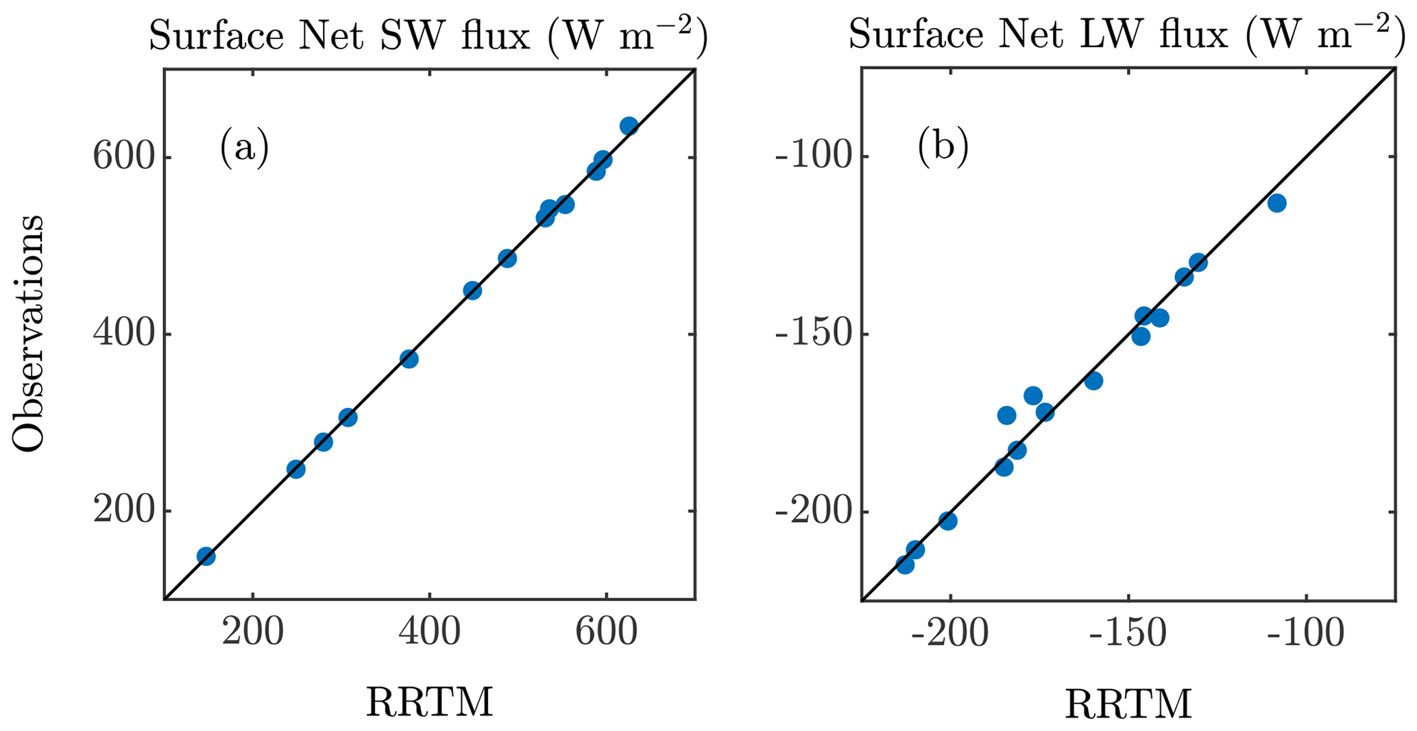
Figure 9Comparison of measured (vertical axes) and bias-corrected modeled (horizontal axes) surface net radiative flux in the (a) SW and (b) LW during times when radiosondes were launched from the field site. The 1-to-1 line is also shown (black).
We also estimate the uncertainty in modeled net surface fluxes during dust storms and for times when we do not have measurements from radiosondes, which includes 1964 and 43 observations at the surface and TOA, respectively. For these cases and in the SW and LW we note good agreement between the modeled and measured fluxes, as evidenced by correlation coefficients of 0.99 and 0.85 for the surface SW and LW flux comparisons (Figs. 10a, b) and 0.97 and 0.93 for the TOA SW and LW flux comparisons (Fig. 10c, d). We note biases in the modeled surface SW and LW fluxes of 4 and 7 W m−2, as well as −56 and −21 W m−2 for the modeled SW and LW fluxes at TOA. The bias-corrected RMSEs for the net SW and LW surface fluxes are 17 and 18 W m−2 and for the net SW and LW TOA fluxes are 26 and 13 W m−2, respectively.
It is likely that the model flux RMSEs for the cases when radiosondes are available are less than that for time periods when radiosondes were not available because of the better representation of the vertical structure of the atmosphere and because we corrected any obvious errors in the ceilometer extinction profiles for the times radiosondes were launched. Furthermore, it is also likely that the RMSE and biases for the TOA fluxes are larger than those at the surface because the satellite footprints cover a wide area that can span different surface types and atmospheric conditions (Fig. 4). We note that the errors in the modeled fluxes were poorly correlated with the accompanying τ, where r2 values remained below 0.02 for all the flux comparisons. The relative RMSE values reported in Fig. 10 are used to estimate error in the RRTM output fluxes in subsequent estimation of the dust direct radiative effect and forcing efficiency.
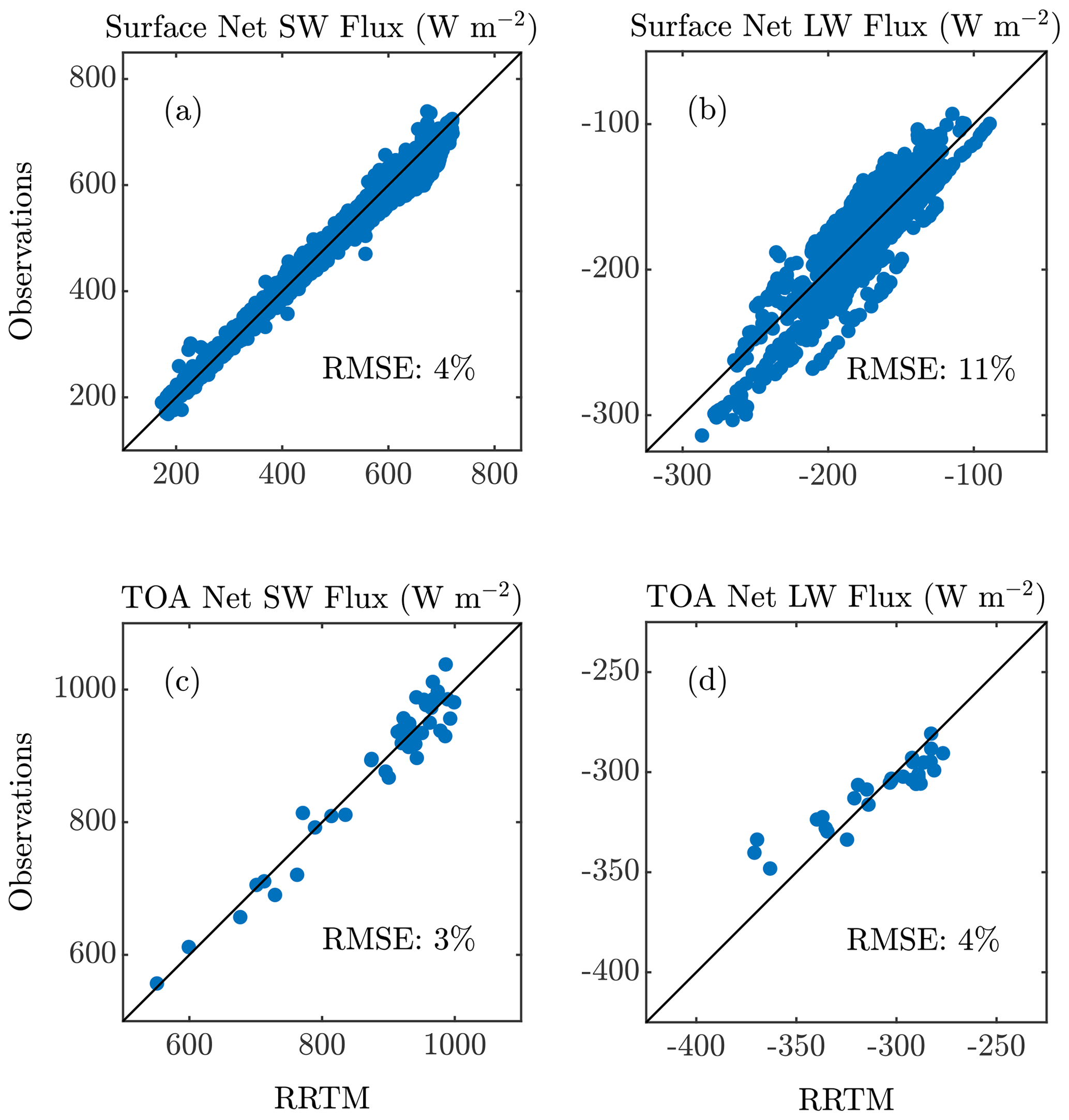
Figure 10Comparison of measured (vertical axes) and bias-corrected modeled (horizontal axes) surface (a, b) and TOA (c, d) net radiative fluxes in the (a, c) SW and (b, d) LW. The 1-to-1 black line and the relative modeled flux RMSE are also shown in each plot. We note that the axes for each panel are distinct.
3.2 Linear model and uncertainty
We develop a linear model of net SW flux at the surface S0 and TOA S∞ in order to generate observational estimates of the SW dust forcing efficiency and direct radiative effect. The advantage to using such a method to estimate the SW dust forcing efficiency and direct radiative effect is that assumptions about the microphysical and single-scattering properties of dust are not required, which are necessary in order to estimate the direct effect via a radiative transfer model (Kuwano and Evan, 2022).
In order to generate observation-based estimates the SW dust forcing efficiency and direct radiative effect we assume that these fluxes can be approximated as linear functions of τ, Pw, cosine of the solar zenith angle μ, and surface SW albedo α:
and
where the S* terms are constants representing net fluxes for a pristine and dry atmosphere over a completely absorbing surface with the sun at the horizon, and the terms are the sensitivities of the net solar fluxes to the independent variables. These sensitives and constants can be estimated via multivariate linear regression given measurements of S0 or S∞, Pw, μ, and α.
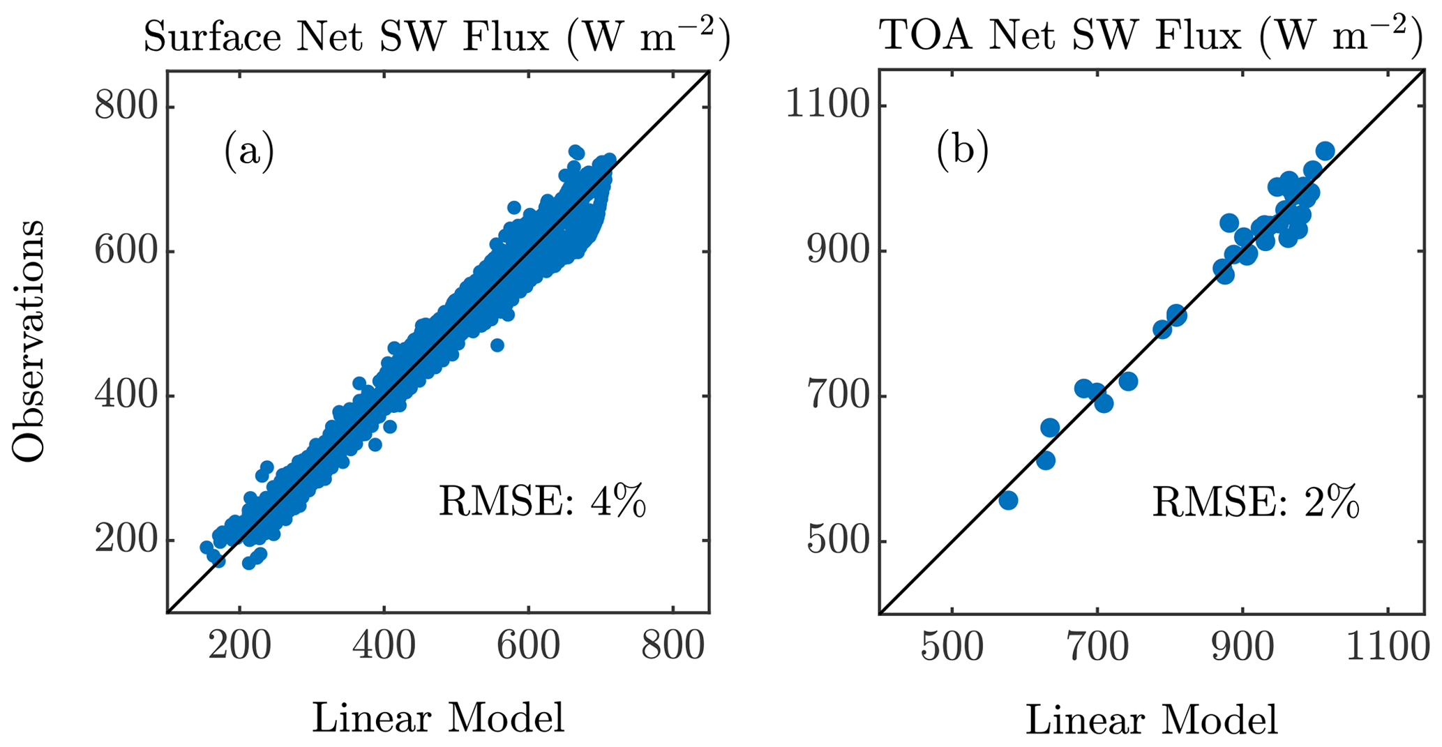
In order to justify these linear models of solar fluxes and quantify the uncertainty in each, we estimate the sensitivity terms and S* in each using simultaneous measurements of S, τ, α, and Pw from the field site (Eq. 4) and satellites (Eq. 5). These fluxes are the same data as used to evaluate the RRTM output (Fig. 10a,c), which include approximately 1964 observations at the surface and 43 observations at TOA. We then calculate surface and TOA net solar fluxes via these linear models. A comparison of the measured and modeled fluxes suggests that the linear model is able to reproduce much of the variability in the measured fluxes (Fig. 11). The percent variances of the observations that are explained by the linear models (i.e., r2 value) and their RMSE are 98 % and 20 W m−2 (4 % relative error) at the surface and 97 % and 20 W m−2 (2 % relative error) at TOA, respectively.
In this section we present and discuss the dust direct radiative effect and forcing efficiencies obtained from the linear (in the SW) and radiative transfer (in the SW and LW) models.
4.1 Observational estimates of the SW instantaneous direct radiative effect and forcing efficiency
We start by estimating the SW dust direct radiative effect and forcing efficiency using only observational data.
4.1.1 Observational methodology
This method to estimate the instantaneous dust direct radiative effect and forcing efficiency is a modified version of that described in Kuwano and Evan (2022). Firstly, the clear-sky direct radiative effect of dust ζ is defined as the difference between the net clear-sky F and pristine-sky Fp fluxes,
In the SW part of the spectrum F can be approximated at the surface or TOA via Eqs. (4) and (5), and pristine-sky fluxes are obtained by setting τ=0 in each. The resultant SW dust direct radiative effects at the surface ζ0 and at TOA ζ∞ are then
and
The dust forcing efficiency is defined as the direct radiative effect per unit optical depth, which in the SW at the surface or TOA are the sensitivity terms in Eqs. (7) and (8), respectively. The atmospheric components of the direct radiative effect and forcing efficiency are interpreted as the differences between the TOA and surface values, where uncertainty is obtained by adding the surface and TOA uncertainties in quadrature. This approach implicitly assumes a horizontally homogeneous atmosphere and surface, which is a limitation of the approach.
We utilize a Monte Carlo approach to quantify the uncertainty in the observational estimates of the SW direct radiative effect and forcing efficiency. Specifically, we repeatedly estimate the terms in Eqs. (4) and (5), adding random error to each of the terms derived from Gaussian probability distribution functions having a mean of zero and standard deviations equal to the uncertainties indicated in Table 1. The uncertainties reported here represent the 95 % confidence interval about the means.
4.1.2 Observational results
The instantaneous SW dust direct radiative effect and forcing efficiency generated from surface and satellite measurements are shown in Fig. 12. At the surface the SW direct radiative effect is W m−2, which corresponds to a forcing efficiency of W m−2 τ−1, and which suggests surface cooling due to scattering and absorption of dust in the atmosphere. At the TOA the SW direct radiative effect is W m−2 and the accompanying forcing efficiency is W m−2 τ−1, which represents cooling by scattering of sunlight back out to space by dust. The relatively larger uncertainty in the TOA forcing values compared to the surface is related to the number of observations available to calculate each: nearly 2000 at the surface and just over 40 at TOA. The atmospheric direct radiative effect and forcing efficiency are 5±6 W m−2 and 30±32 W m−2 τ−1, representing heating by dust mainly due to absorption by iron oxides in the aerosols (Fig. 6).
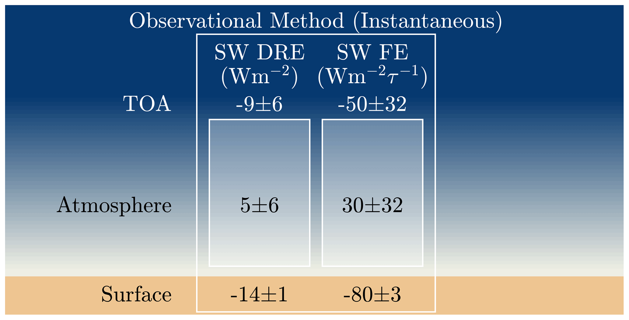
Figure 12Surface and satellite-based observational estimates of the clear-sky instantaneous SW direct radiative effect (DRE) and forcing efficiency (FE) at the surface, in the atmosphere, and at TOA. The reported uncertainties represent the estimate's 95 % confidence intervals.
4.2 Model estimates of the SW and LW instantaneous direct radiative effect and forcing efficiency
We next estimate both the SW and LW dust direct radiative effect and forcing efficiency using output from the RRTM simulations (Sect. 3.1).
4.2.1 Model methodology
The SW and LW dust direct radiative effect is obtained from the differences of the modeled surface or TOA clear- and pristine-sky fluxes (e.g., Eq. 6). Forcing efficiencies (the sensitivities in Eqs. 7 and 8) are then estimated by regressing τ onto these direct radiative effect values. We repeat this procedure with output from the RRTM simulations representing the most and least absorbing cases to estimate the uncertainty in the model estimates of the direct effect. We combined these uncertainties, in quadrature, with the root mean squared errors derived from the comparison to the observational data (Fig. 10).
4.2.2 Model results
The instantaneous dust direct radiative effect values generated from the radiative transfer model output are shown in Fig. 13. In general, the modeled SW direct radiative effect suggests much stronger absorption by dust than is implied by the observational results (Fig. 12), with a modeled atmospheric direct effect of 20 W m−2, which is a factor of 4 larger than the 5 W m−2 derived from the observational estimate. Consequently, the modeled SW TOA direct effect is much smaller in magnitude (−1 W m−2) than that from observations (−9 W m−2). The modeled and observed surface direct effects show relatively less disagreement, since the surface forcing is, to first order, most dependent on extinction, which does not vary as strongly as the single-scattering albedo. These results imply that the soil iron oxide content retrieved from AVIRIS-C may be too large, which is consistent with recent findings that the retrieval algorithm generates an iron oxide content that is too high at the global scale (Philip Brodrick, personal communication, 15 May 2024). Indeed, the modeled SW direct effect agrees to within 1 W m−2 of the observational estimates for the least absorbing case (i.e., the upper limit of the single-scattering albedo in Fig. 8a), which corresponds to −14, −8, and +6 W m−2 at the surface, at TOA, and in the atmosphere, respectively. These findings are consistent with other studies that highlight the role of iron oxides in determining the SW dust direct effect (e.g., Li et al., 2021).
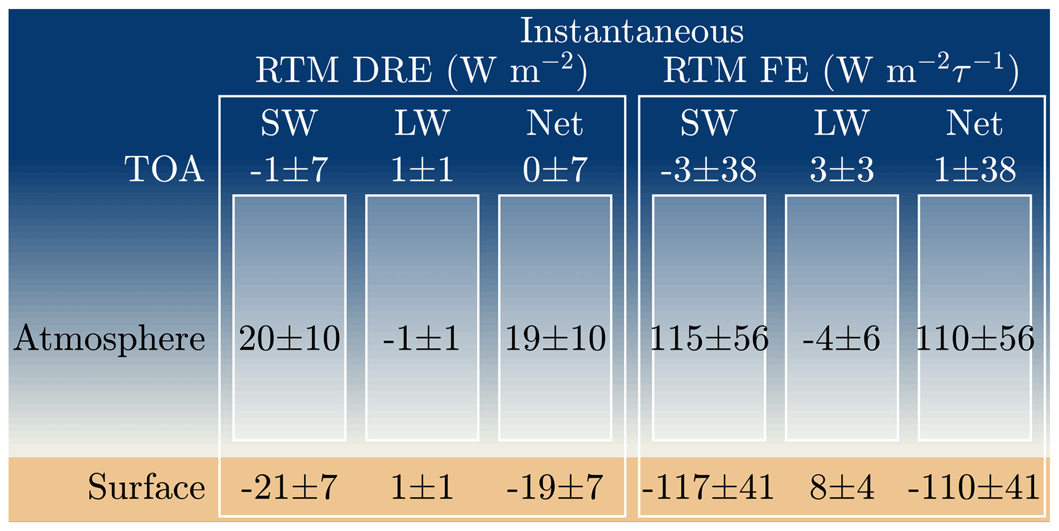
Figure 13Shown are estimates of the clear-sky instantaneous SW, LW, and net dust direct radiative effect (DRE, left) and forcing efficiency (FE, right) generated from the radiative transfer model (RTM) simulations. The reported uncertainties represent the estimate's 95 % confidence intervals.
In the longwave part of the spectrum the dust direct radiative effect is small in magnitude, mainly owing to the relatively shallow dust layers that are typical of dust storms passing over the field site (Evan et al., 2023); the average depth of dust storms passing over the field site obtained from the ceilometer is 1.7 km (not shown). We obtain a modest surface and TOA direct effect of 1±1 W m−2, with a resulting atmospheric direct effect of W m−2. The LW forcing efficiencies are approximately equivalent to the direct effect values divided by the mean dust optical depth of 0.18. The relatively smaller uncertainty in the LW direct effect, when compared to that in the SW, is due to the small uncertainty in the LW extinction coefficient (Fig. 8).
We estimate the instantaneous net dust direct radiative effect and forcing efficiency by summing the SW and LW components (Fig. 13). At TOA, the modeled LW and SW direct effects cancel, although the uncertainty is ±7 W m−2. Thus, the model output is not informative with regards to the climate forcing of dust. The sign of the modeled net direct effect at the surface and within the atmosphere is constrained by the model, giving values of and 19±10 W m−2. These results are consistent with findings from other studies that the net effect of dust is to warm the atmosphere and cool the surface, potentially increasing atmospheric stability (e.g., Miller et al., 2004). We can alternatively estimate the net dust direct radiative effect by summing the observed SW and modeled LW values. By doing so we obtain a net direct effect of W m−2 at the surface, W m−2 at TOA, and 6±6 W m−2 in the atmosphere. These results would suggest that dust has a net cooling effect at TOA, at least during daytime, with surface cooling and likely atmospheric warming.
4.3 Annually averaged dust direct radiative effect
We next estimate an annually and diurnally averaged dust direct radiative effect for clear-sky conditions using the output from RRTM SW and LW based on monthly and 15 min averaged in situ and reanalysis data. To do so we conducted simulations with RRTM over 24 h periods corresponding to the 15th day of each calendar month at a 15 min temporal resolution. We define the vertical structures of pressure P(z) and specific humidity q(z) by averaging over the profiles collected from the radiosondes launched at the field site during dusty conditions (Tables 1 and A1). We then estimate monthly values for each by scaling those profiles by monthly averages of the field site station surface pressure or GPS-retrieved Pw, generated for data collected over the 2020–2022 time period. We prescribe the vertical profile of dust extinction based on the ceilometer profiles corresponding to the radiosonde launches and then scale these by the long-term mean dust optical depth of 0.18. Our data suggest a relatively small diurnal cycle in this value, and additional simulations with RRTM where we prescribe a dust diurnal cycle based on measurements had little effect on the calculated direct effect and forcing efficiency. We estimate 15 min averaged soil temperature (z=0 m) retrieved from observations of LW upward flux and 1 m air temperature in a similar fashion from the site meteorological station. We obtain vertical profiles of temperature directly from the JRA-55 reanalysis on the 15th of each month averaged over the 2020–2022 time period. Since the lowest height of the reanalysis air temperature is approximately 60 m a.g.l., we interpolate temperatures between these heights using the measured 1 m air temperature. We assume constant surface SW and LW albedos. We calculate the annual and diurnally averaged dust direct radiative effect and forcing efficiency directly from the model output. We estimate uncertainty in a manner identical to that described for the instantaneous calculations, including repeated RRTM calculations using the more and less absorbing single-scattering properties (Fig. 8)
The estimates of the clear-sky annually and diurnally averaged SW, LW, and net dust direct radiative effect and forcing efficiency at the surface and TOA and in the atmosphere are shown in Fig. 14. The largest discrepancy between the instantaneous and diurnally and annually averaged values is in the SW at the surface, with values that are approximately half those from the instantaneous calculations (Fig. 13), which is due to averaging over the nighttime hours when there is no solar insolation. At TOA we do not see a similar reduction in the SW direct radiative effect or forcing efficiency because of the nonlinear response in the direct radiative effect to changes in the solar zenith angle associated with the particle asymmetry factor (Fig. 8b); at low solar zenith angle (i.e., the sun is overhead), the direct effect can become positive due to the strong forward scattering of dust. At higher solar zenith angles, when the sun is lower in the sky but the solar insolation is still large, the direct radiative effect is at a maximum negative value. The average solar zenith angle corresponding to the instantaneous calculations is 50°, which corresponds to a regime where the direct radiative effect is negative but not at a maximum value and which happens to be approximately equal to the diurnal average.
The model results suggest that over land and close to source regions dust cools the climate, as evidenced by the net direct effect value of W m−2. There is also a net cooling at the surface of W m−2 and warming of the atmosphere of 8±4 W m−2. If we again assume that the RRTM simulations corresponding to the less absorbing case are closer to the actual direct effect, then we obtain an SW direct effect of −7, −5, and +2 W m−2 at the surface, at TOA, and in the atmosphere. Using those values to obtain a net effect, we estimate a TOA direct effect of −6 W m−2, implying that dust has a cooling effect at TOA.
We note that the direct effect values in Fig. 14 correspond to τ=0.18, which is the average daytime τ during dust storms. The actual diurnally and annually averaged direct effect is smaller in magnitude and would be obtained by scaling these estimates by the fractional amount of time that dust is present in the atmosphere. However, we are unable to do so since we cannot reliably identify dust storms during the nighttime hours and because we do not identify all dust events passing over the field site. However, the forcing efficiencies also reported in Fig. 14 are, to first order, independent of τ and are thus potentially more useful in terms of comparing study results.
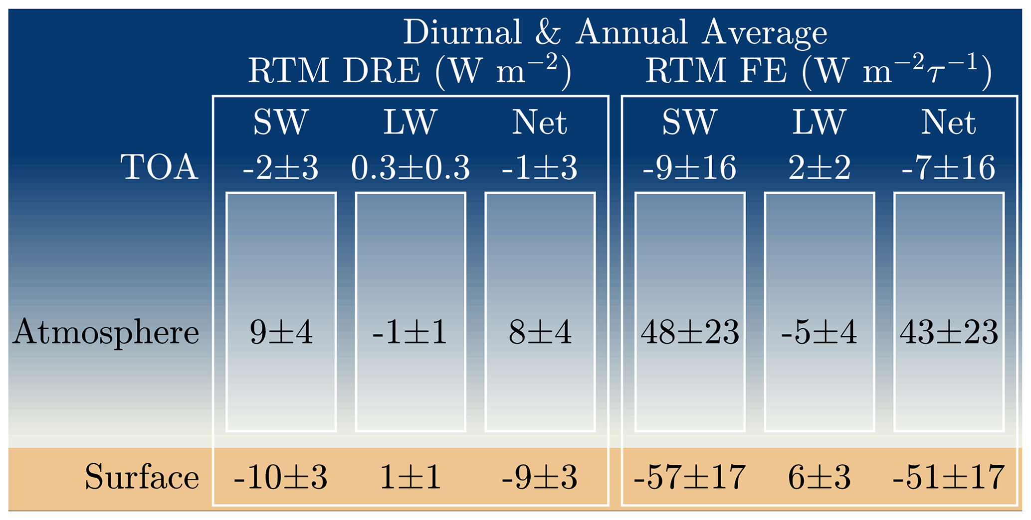
Figure 14Clear-sky annually and diurnally averaged SW, LW, and net direct radiative effect and forcing efficiency of dust at the surface, at TOA, and in the atmosphere, estimated from simulations with a radiative transfer model (RRTM). Uncertainties represent the 95 % confidence interval and are based on the uncertainties in the instantaneous values (Fig. 13).
We next compare our estimates of the direct radiative effect and forcing efficiency with values from other observational and model studies.
5.1 Instantaneous SW comparisons
We begin by comparing our estimates of the SW instantaneous forcing efficiency with observational values estimated at the TOA over the Sahara (Kuwano and Evan, 2022), over Lampedusa at the surface (di Sarra et al., 2013), and at the surface and TOA (Di Biagio et al., 2010, study locations in Fig. 15a). Each of these studies reports forcing efficiency values averaged over discrete solar zenith angle ranges, so for these comparisons we recalculated the forcing efficiency estimated from the field site for those same zenith angle ranges.
The surface SW forcing efficiency calculated from our study over the μ range of used in di Sarra et al. (2013) is W m, which is approximately two-thirds the value of W m reported in their study (Fig. 15b). Similarly, over the μ range of used in Di Biagio et al. (2010), we obtain a forcing efficiency of W m, which is less than two-thirds the value of W m reported in their study (Fig. 15c). We speculate that there are two main reasons for the discrepancies in the surface SW forcing efficiency estimates. Firstly, the Lampedusa studies included surface albedo values corresponding to both land and water-covered surfaces, whereas for this study we limited our study region to footprints that were mostly over land (Fig. 4). As the surface albedo decreases the contrast between clear-sky and dusty scenes increases, resulting in a larger (in magnitude) forcing efficiency. Secondly, it is also likely that methodological differences also play a role in the discrepancy. Both studies adopted the methods of Satheesh and Ramanathan (2000) to calculate the forcing efficiency, which is equivalent to neglecting the water vapor Pw, cosine of the solar zenith angle μ, and albedo α terms in Eq. (4). As such, if τ is correlated with these terms the resulting forcing efficiency may be biased (Kuwano and Evan, 2022). Furthermore, the criteria for selecting dust in also different; in these two studies dusty scenes are mainly identified via Ångström exponent thresholds. If we calculate the surface SW forcing efficiency following the methods described in Di Biagio et al. (2010) we obtain a forcing efficiency of W m, which is significantly closer to their estimate of (not shown). If we also artificially adjust the surface albedo in our calculations to be half the observed value (approximately 0.15 rather than the observed 0.3), then we obtain an SW forcing efficiency of W m, which is in agreement with that from Di Biagio et al. (2010). Thus, it is plausible that differences in methodology and environmental characteristics are the main causes of disagreement in the SW forcing efficiency estimates rather than differences in the actual radiative properties of the dust.
In order to ensure sufficient data for the remaining comparisons discussed in this section, we use output from RRTM to simulate the SW forcing efficiency at the TOA, which is justified given the agreement between our observation- and model-based estimates of the SW forcing efficiency (Figs. 12, 13). Here, we estimate the uncertainty in the RRTM output as the difference between repeated RRTM calculations using the more and less absorbing single-scattering properties, with the absolute uncertainties shown in the subsequent figures. The instantaneous SW TOA forcing efficiencies from Di Biagio et al. (2010) and Kuwano and Evan (2022) are and W m, respectively, whereas we obtain a value of 33±64 W m averaged over the solar zenith angle range of roughly 0–45° (μ from 0.7–1, Fig. 15c). We speculate that, similar to the case for the surface, the disagreement in TOA forcing efficiency is at least in part due to methodological differences. For example, we recalculated the TOA forcing efficiency from Kuwano and Evan (2022), also accounting for variations in surface albedo and μ (e.g., Eq. 8), obtaining a value that was slightly smaller in magnitude (−12 W m) and closer to the value obtained here. Within the atmosphere the forcing efficiencies from this study of 131±64 W m and from Di Biagio et al. (2010) of 129±23 W m are in better agreement than at the surface or TOA.
Overall, the studies compared here agree that the SW forcing efficiency of dust at the surface is negative and at TOA is relatively smaller in magnitude and close to zero, resulting in a positive atmospheric forcing efficiency. These characteristics are consistent with weakly absorbing aerosols that have minimal TOA radiative effect and that increase solar absorption in the atmosphere at the expense of the downwelling solar flux at the surface.
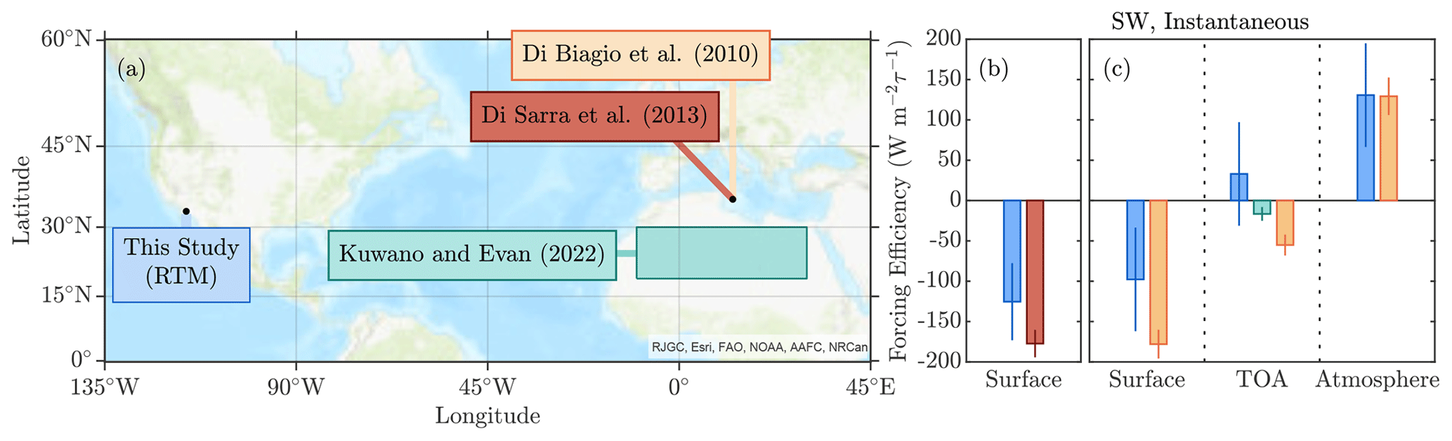
Figure 15(a) Map of the locations or regions used to calculate the SW forcing efficiency of dust in this and three other studies (Di Biagio et al., 2010; di Sarra et al., 2013; Kuwano and Evan, 2022). The corresponding SW forcing efficiency values at the surface, at TOA, and in the atmosphere averaged over the μ intervals (b) 0.34–0.8 and (c) 0.7–1, where colors of the bars are referenced to the colors of the text boxes and their studies indicated in (a).
5.2 Instantaneous LW comparisons
We next compare our instantaneous LW dust forcing efficiency estimates with those from seven other studies. The locations of all studies compared here are shown in Fig. 16a. Similarly to this study, Hansell et al. (2012) used observations and retrievals to constrain radiative transfer model estimates of the LW direct radiative effect during a 2-week dust storm in Zhangye, China. We then estimated an equivalent forcing efficiency based on their reported mean dust storm optical depth of 0.5. We find statistical agreement between our estimates of the LW instantaneous forcing efficiency of 8±4 W m and that from Hansell et al. (2012) of 19±9 W m (Fig. 16b). At the TOA we find that our estimate of 3±3 W m is also in agreement with the value of 10±7 from Hansell et al. (2012), as well as that from Brindley and Russell (2009) of 14±10 W m, corresponding to the Saada, Morocco, location (BR09e in Fig. 16a). Otherwise, the other 13 reported values of the TOA instantaneous LW forcing efficiency are all statistically larger than what we report here, with values ranging from 12 W m (Song et al., 2022) to 36 W m (Hsu et al., 2000) (Fig. 16b). The average forcing efficiency from all studies we compare our results to is 20±6 W m, where we note that the uncertainty is poorly constrained since several studies did not report an uncertainty range. We note that the Hansell et al. (2012) TOA and surface values imply an atmospheric LW forcing efficiency of W m, which agrees with our value of W m.
It is difficult to precisely ascertain the causes of the differences in the LW instantaneous forcing efficiency at TOA. However, the relatively shallow depth of dust over the field site may at least partially explain why our value of the forcing efficiency is smaller than that from these other studies. For example, Hansell et al. (2012) reported an average dust scale height of 3 km during their study, whereas we rarely observed dust layers extending beyond a height of 2 km (e.g., Evan et al., 2023).
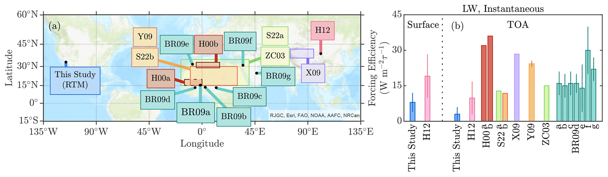
Figure 16(a) Map of the locations or regions used to calculate the LW forcing efficiency of dust in this and seven other studies: Hansell et al. (2012, H12), Hsu et al. (2000, H00a,b), Song et al. (2022, S22a,b), Xia and Zong (2009, X09), Yang et al. (2009, Y09), Zhang and Christopher (2003, ZC03), and Brindley and Russell (2009, BR09a–g). (b) The corresponding LW forcing efficiency values at the surface and TOA, where colors of the bars are referenced to the colors of the text boxes indicated in (a).
5.3 Comparison of diurnal and annual average SW forcing efficiencies
Lastly, we compare estimates of clear-sky diurnally and annually averaged SW forcing efficiency at the surface, at TOA, and in the atmosphere between this and seven other studies (study locations in Fig. 17a). The annually and diurnally averaged SW forcing efficiency at the surface estimated from this study is W m (Fig. 17b, blue) and is statistically similar to the values of and W m reported by Zhou et al. (2005), W m estimated from Valenzuela et al. (2012), and W m found in García et al. (2014). The results from the other studies shown in Fig. 17 (Di Biagio et al., 2010; Ge et al., 2010; di Sarra et al., 2013) all report surface forcing efficiencies that are significantly more negative than what we find, with a multi-study mean value of W m. We speculate that, similar to the case for the instantaneous forcing efficiency (Fig. 15), at least part of this discrepancy is due to methodological differences.
At the TOA our SW forcing efficiency of W m is in agreement with the values of and W m from Zhou et al. (2005) and W m from Valenzuela et al. (2012) (Fig. 17b). Similar to the instantaneous case, the TOA forcing efficiency from Di Biagio et al. (2010) of W m is 5-fold larger in magnitude than what we report. For these same four studies we also calculated the atmospheric forcing. Here we find agreement in our estimate of 48±23 W m and those from Zhou et al. (2005), Di Biagio et al. (2010), and Valenzuela et al. (2012), which are 36±14, 32±11, 32±7, and 57±14 W m, respectively.
When averaging across all studies, we obtain an observation-based SW forcing efficiency of , , and 38±11 W m at the surface, at TOA, and in the atmosphere, respectively. Based on these values, the SW direct radiative effect at TOA is 3±1 times larger in value than that at the surface, implying that the SW surface cooling by dust is not balanced by the relatively weaker heating in the atmosphere, resulting in a negative direct effect at TOA. These results also underscore the importance of quantifying the iron oxide content in dust, since these minerals drive solar absorption and thus strongly affect the balances in Fig. 17b (Di Biagio et al., 2019). We are not able to generate an equivalent estimate of the annual and diurnally averaged LW forcing efficiency from the studies represented in Fig. 16 since they do not report these values.
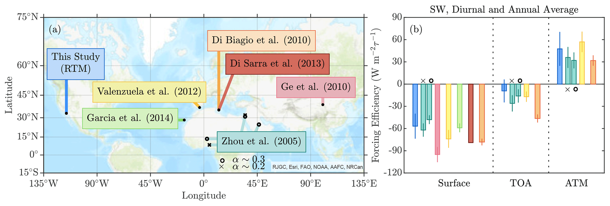
Figure 17(a) A map of the locations or regions used to calculate the diurnally and annually averaged SW forcing efficiency of dust for this and six other studies. (b) The corresponding SW forcing efficiency values at the surface, at TOA, and in the atmosphere, where colors of the bars are referenced to the colors of the text boxes and their studies indicated in (a).
In this study we used both observations and model output to generate estimates of the dust direct radiative effect in the American Southwest. To do so, radiometric and meteorological measurements were obtained over a 3-year period at a field site located in the northwestern Sonoran Desert (Fig. 1). We developed a novel method to estimate the dust SW forcing efficiency and direct radiative effect via our observations alone to generate new estimates of these values at the surface, at TOA, and in the atmosphere (Fig. 12). We generated estimates of the dust refractive index using surface soil mineralogy products from AVIRIS-C (Figs. 6, 7) and then used these data to model clear-sky fluxes over the field site with RRTM (Figs. 9, 10). We then used RRTM to simulate the SW dust direct radiative effect, obtaining agreement between the modeled and observational values within their respective uncertainties (Fig. 13). However, our results also implied that the iron oxide soil content was too high in the AVIRIS-C retrievals, evidenced by the much stronger SW atmospheric absorption in the model. We also used RRTM to quantify the dust forcing efficiency and direct effect in the LW (Fig. 13). Since the magnitude of the SW direct effect is 6–10 times larger than that in the LW, we obtained a net direct radiative effect of W m−2 at TOA that is balanced by a surface cooling of W m−2 and atmospheric heating of 8±4 W m−2 (Fig. 14). However, when combining the observation-based SW direct effect estimates and the RRTM-based LW estimates, we obtain a net direct effect of W m−2, suggesting that, during daytime hours, dust has a net cooling effect.
We compared our estimates of the instantaneous and diurnally and annually averaged dust forcing efficiencies with values from a number of other studies that estimated these values over specific locations or regions using in situ measurements and satellite retrievals. We found that in the SW, our observation-based results were more positive at the surface and TOA than those from three other studies (Fig. 15), although methodological differences may contribute to the disagreement. We also expanded this comparison of the model-based SW forcing efficiency to annually and diurnally averaged values (Fig. 17). Here we found agreement between our estimates and that from several other studies at the surface, at TOA, and in the atmosphere, although we found that the magnitude of the SW forcing efficiency from our study was smaller than that from the majority of the other studies, which at TOA is at least partially explained by the dust optical properties that are likely too absorbing in our RRTM simulations. We also compared our estimates of the LW instantaneous direct effect with that from other studies, finding that at the surface and at the TOA our LW forcing efficiency was smaller in magnitude than that from these other studies (Fig. 16). Although it is plausible that methodological differences play a role in differences in the LW forcing efficiencies, the relatively shallow nature of the dust layers advected over the field site (e.g., Fig. 5) relative to that of these other studies is likely a significant underlying cause.
In situ and observation-based estimates of the dust direct effect are valuable in terms of understanding how changes in dust concentration affect the radiative energy balance at a local scale. These data are also valuable at the global scale as they provide an observational constraint on estimates of the direct radiative effect from climate models. However, the apparent sensitivity of the observation-based estimates of the SW direct radiative effect to methodology inhibits the utility of these data as a check on model output. As such, and at least in the SW, our results imply that there is a need to adopt a standardized methodology, or at least a standard set of data to be collected, in order to generate data of maximal utility for evaluating model output. We suggest that the parameters measured and retrieved in Eqs. (4) and (5) represent a reasonable set of data that, in this linear framework, account for variability in factors that affect the estimated direct radiative effect. Additionally, a standardized methodology to identify dust from, for example, sun photometers, would also be useful in terms of comparing results among observational studies. Furthermore, it is plausible that a simulator, much like the satellite simulator used to compare cloud cover from climate models and satellites (Klein and Jakob, 1999), could be developed in order to improve the capacity to evaluate model estimates of the dust direct radiative effect.
As discussed in Sect. 2.1.1, one pyranometer was factory-calibrated prior to (2018) and after (2023) acquisition of data for this project, for which the calibration coefficients differed by 1.5 % (10.95 and 11.12 µV W−1 m2, respectively). We then calibrated the other instrument by placing the two side by side in the upward-looking direction for time spans ranging from 1–3 weeks either in La Jolla, CA, or at the field site. We filtered the data consistent with the factory calibration of the reference pyranometer, including only using measurements for solar zenith angle <50 degrees, downward solar flux >500 W m−2, and when the relative difference in the fluxes between the instruments was <3 %. We calculated a cross-calibration coefficient as the slope of the least-squares linear regression of the factory-calibrated voltage onto that for the field-calibrated instrument, forcing the line through the origin to be consistent with the manufacture's instructions. The resulting cross-calibration coefficients were 1.08 and 1.09 (Fig. B1), all with uncertainties, defined via the 95 % confidence interval in the regression slopes, of 0.01 %. The resultant calibration coefficients for the field-calibrated instrument (factory calibration coefficient multiplied by the cross-calibration coefficient) were then 10.13, 10.10, 10.10, and 10.24 µV W−1 m2, corresponding to the 2018, 2021, 2022, and 2023 calibration periods, all having 2σ uncertainties of ±0.001 µV W−1 m2 (0.01 % relative uncertainty).
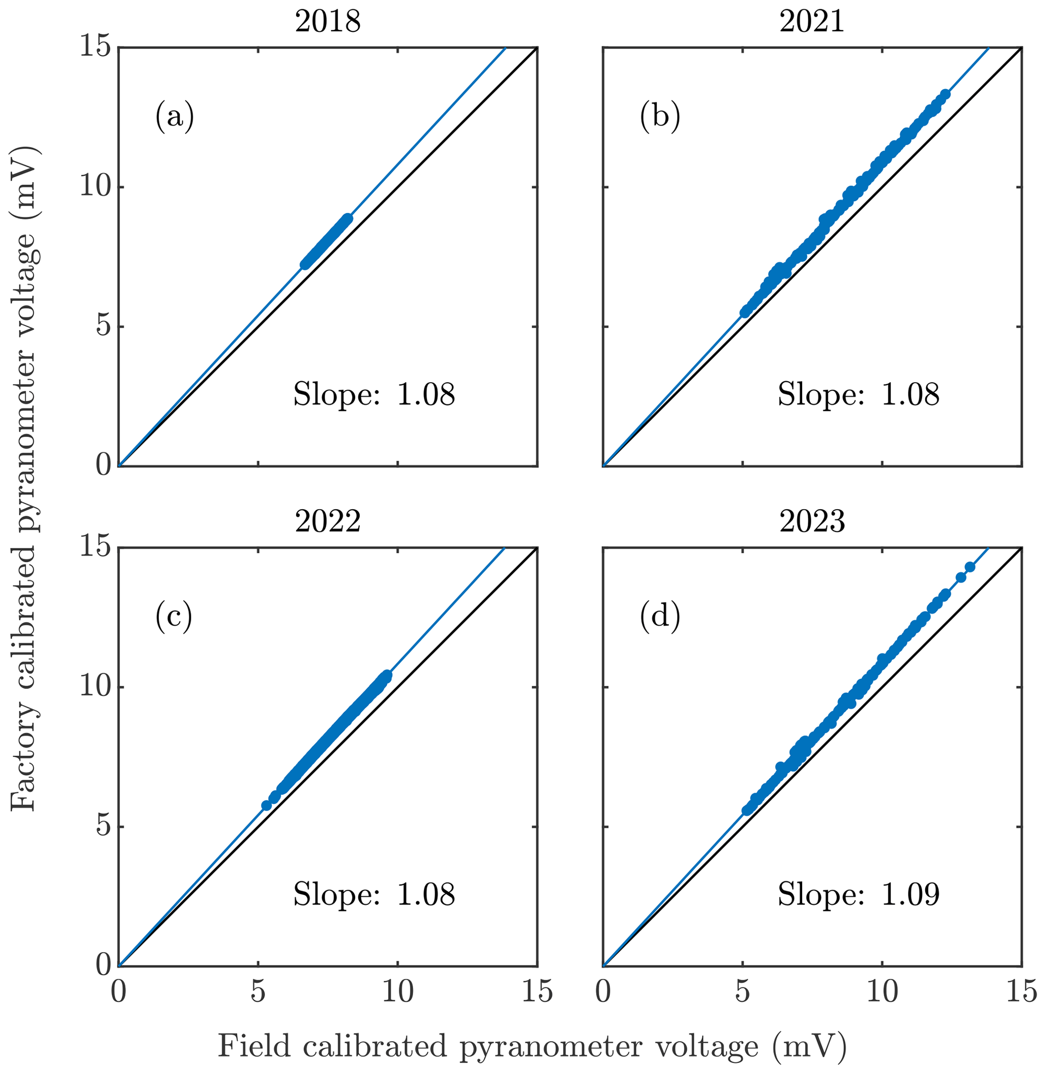
Figure B1Plotted are voltages (filled blue circles) measured from upward-looking mounted pyranometers during cross-calibration activities in (a, b) La Jolla, CA, and at (c, d) the field site. Voltages from the factory-calibrated pyranometer are referenced to the vertical axis, and those from the field-calibrated instrument are referenced to the horizontal axis. The linear least-squares regression lines are plotted in each panel, and the slope of the lines is also indicated (the 95 % uncertainty in each is 0.01 %).
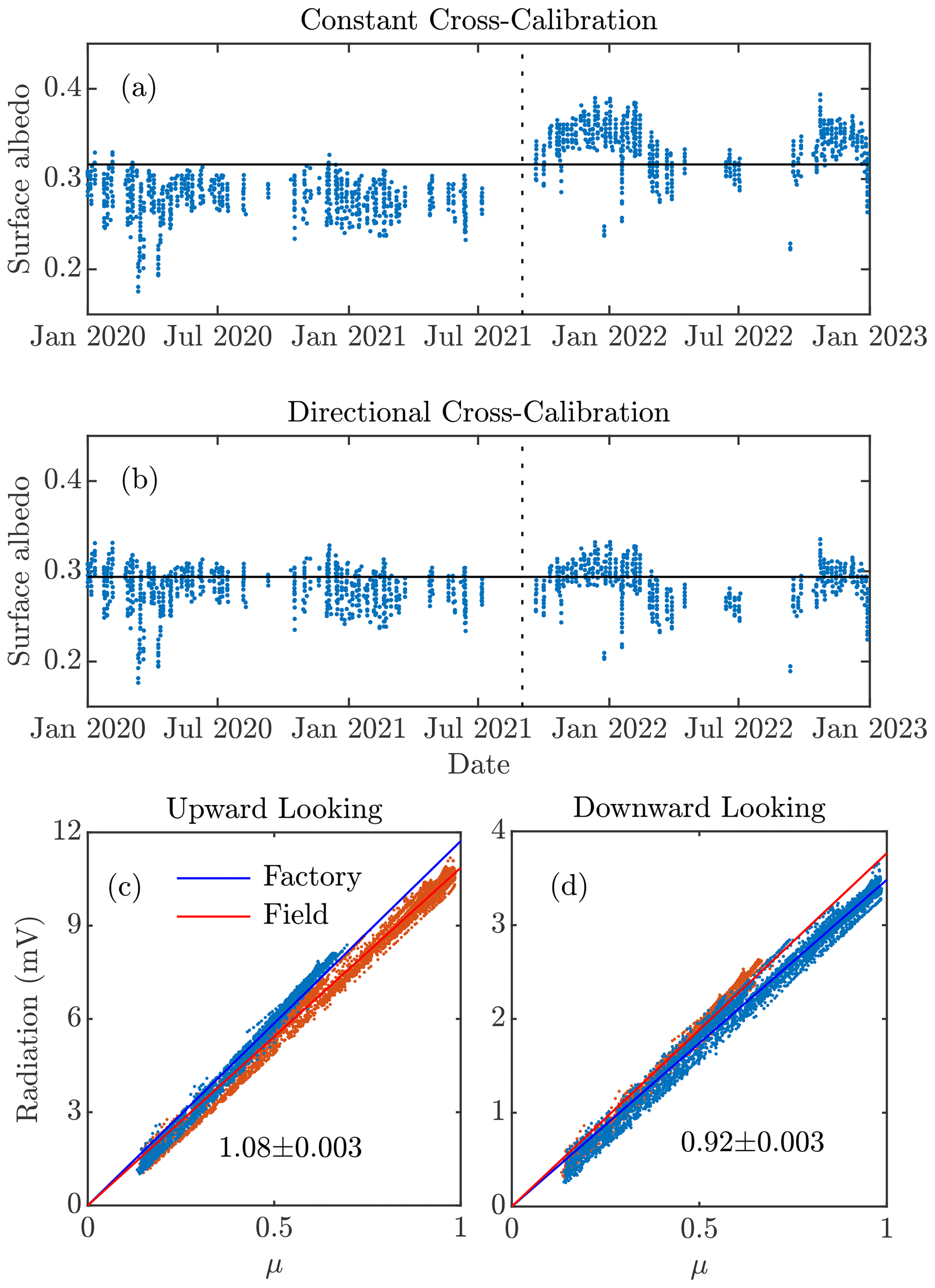
Figure B2(a, b) Time series of surface shortwave albedo generated from voltage measured by upward- and downward-looking pyranometers at the field site. In (a) a constant cross-calibration coefficient is applied to the field-calibrated instrument, and in (b) the calibration coefficient depends on the orientation of the instrument (upward- of downward-looking). Also shown are plots of measured voltage as a function of the cosine of the solar zenith angle μ when both instruments are oriented in the (c) upward- or (d) downward-looking directions. The specific pyranometer (factory- or field-calibrated) is indicated in the legend. Also shown in (c, d) are the linear least-squares best-fit lines, as well as the ratios of these lines and their respective uncertainties.
After cross-calibrating the field-calibrated pyranometer (Fig. B1) we noted that the resulting surface SW albedo showed an apparent upward shift after 1 September 2021 (Fig. B2a), which immediately followed a cross-calibration activity. Prior to this date the factory-calibrated instrument had been oriented in the downward-facing direction (measuring outgoing radiation). However, the instruments had been inadvertently re-installed after this date such that the factory-calibrated instrument was oriented in the upward-facing direction (measuring downwelling radiation). To investigate the source of this apparent bias we examined the measured voltages generated by both instruments during 2020 and 2022 during pristine-sky conditions, which were defined as times when the AERONET-retrieved aerosol optical depth was less than 0.05.
A plot of uncalibrated voltages from the factory-calibrated (measured during 2022) and field-calibrated (measured during 2020) pyranometers, which is when they were oriented in the upward-looking direction, as a function of the cosine of the solar zenith angle μ shows the expected approximate linear relationship between solar flux and μ (Fig. B2c). We interpret the ratio of the slopes of the linear least-squares regression lines for these data, both forced through the origin, as the cross-calibration coefficient (factory slope divided by field slope), which in this case is 1.084±0.005, in agreement with the cross-calibration coefficients in Fig. B1. We note that the uncertainties in these ratios are determined by summing the relative uncertainties in the respective regression slopes in quadrature, which are themselves the 95 % confidence intervals in the regression slopes. When we repeated this analysis using the uncalibrated voltages when both instruments were oriented in the downward-facing direction we obtained a smaller cross-calibration coefficient of 0.920±0.005 (Fig. B2d). Applying the different cross-calibration coefficients to the field-calibrated pyranometer depending on the instrument orientation (1.084 prior to 1 September 2021 and 0.920 after this date) resulted in a pristine-sky surface solar albedo time series that no longer showed an apparent bias around this date (Fig. B2b).
Previous work has speculated that pyranometer orientation could impact instrument calibration (Kohsiek et al., 2007), and our results would suggest this is indeed the case, although the cause is not clear. Future work will explore this calibration issue by generating simultaneous measurements from these instruments when mounted in the upward and then the downward directions. In the meantime, we note that we obtained nearly identical estimates of the dust direct radiative effect and forcing efficiency when using either cross-calibration method (i.e., a constant value or direction-dependent values). As such, we calibrate the field-calibrated instrument by interpolating in time the coefficients derived during the cross-calibration periods when both instruments were mounted in the upward-looking position (Fig. B1).
Turning to the pyrgeometers, one instrument was factory-calibrated along with the pyranometer, for which the calibration coefficients differed by 3 % (13.11 and 12.72 µV W−1 m2, respectively). We then calibrated the second instrument by placing the two side by side in the upward-looking direction similar to what was done for the pyranometers. We filtered the data according to the same criteria used for the factory calibration, including the measured net flux being W m−2, the difference in the instrument temperatures being °C, and the deviation of the resulting downward longwave flux being W m−2. We calculated the cross-calibration coefficient as the slope of the linear least-squares regression of the factory-calibrated voltage onto that for the field-calibrated instrument, forcing the line through the origin. The resulting cross-calibration coefficients were 1.09 or 1.10, all with uncertainties, defined via the 95 % confidence interval in the regression slopes, of less than 0.02 % of the coefficient values (Fig. B3). The resultant calibration coefficients for the field-calibrated instrument (factory calibration coefficient multiplied by the cross-calibration coefficient) were then 12.06, 11.97, and 11.63 µV W−1 m2, corresponding to the 2018, 2021, and 2023 calibration periods, all having 2σ uncertainties of ±0.01 µV W−1 m2 (0.12 % relative uncertainty).
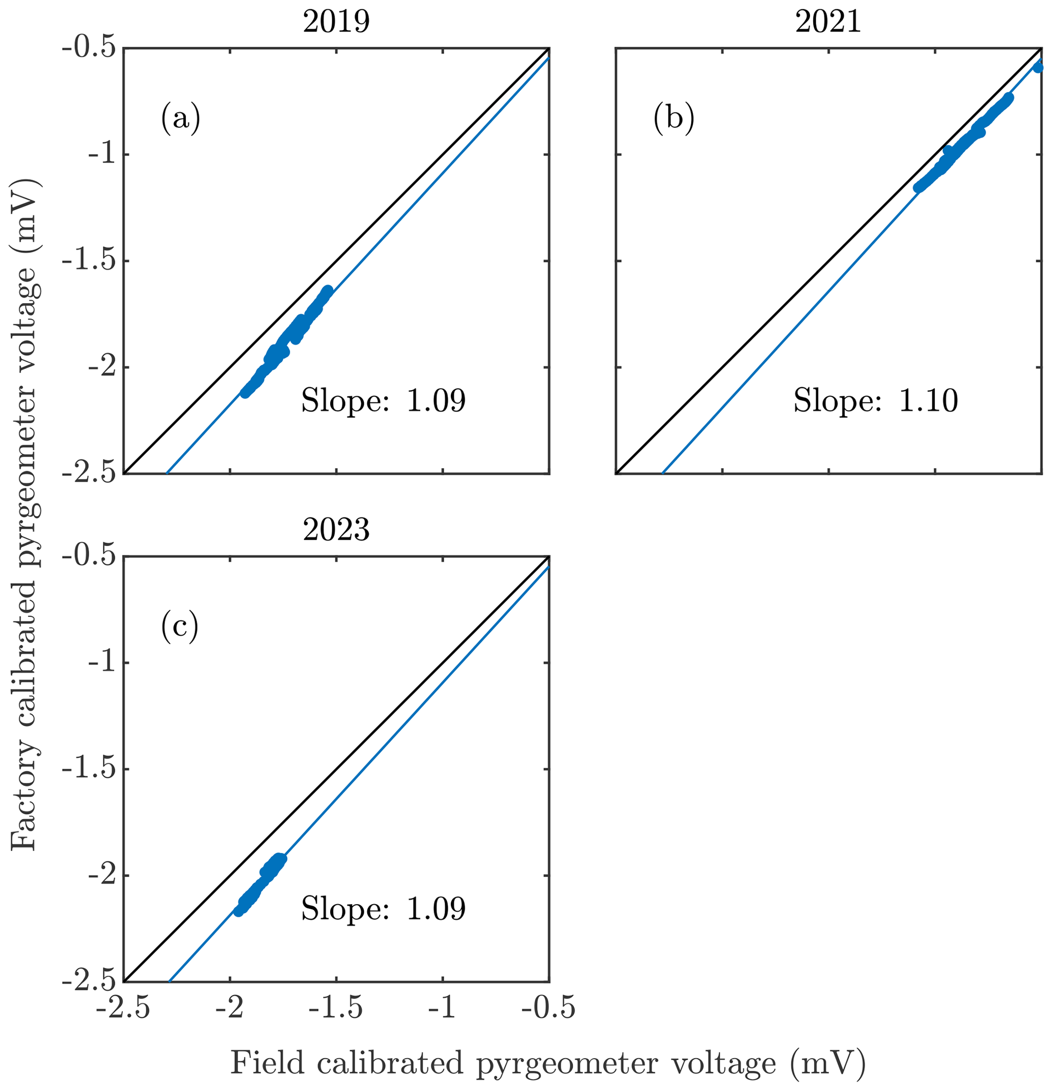
Figure B3Plotted are voltages (filled blue circles) measured from upward-looking mounted pyrgeometers during cross-calibration activities in (a, b) La Jolla, CA, and at (c) the field site. Voltages from the factory-calibrated pyrgeometer are referenced to the vertical axis, and those from the field-calibrated instrument are referenced to the horizontal axis. The linear least-squares regression lines are plotted in each panel, and the slope of the lines and their 95 % confidence intervals are also indicated.
Shown in Fig. C1 are the complex refractive indices for the individual minerals considered when calculating a dust index of refraction and the mean refractive indices for the clay and silicate mineral subgroups (black lines).
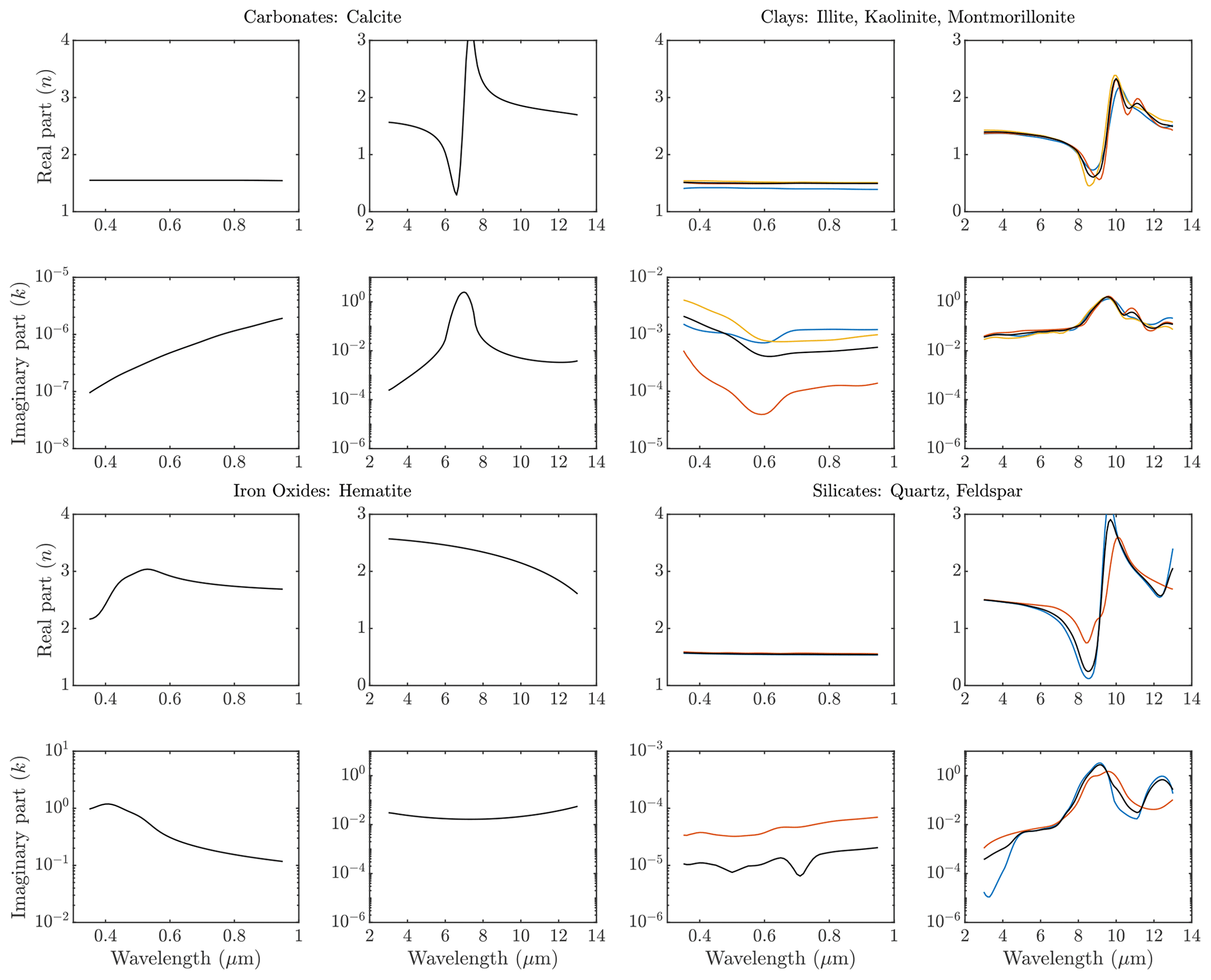
Figure C1Plotted are the real n and imaginary k indices of refraction in the shortwave and the longwave parts of the electromagnetic spectrum, for calcite (top left); hematite (bottom left); the clay minerals (top right) consisting of illite (blue), kaolinite (red), and montmorillonite (yellow); and the silicates (bottom right) consisting of quartz (blue) and feldspar (red). The black lines in the clay and silicate plots represent the volume-averaged means based on the dust abundance of the minerals (Fig. 6)
Measurements obtained from the CERES SSF level 2 data product can be obtained from https://ceres.larc.nasa.gov/data/ (Loeb, 2023). Reanalysis data were acquired from the Japan Meteorological Agency (accessed on 4 May 2023 via https://rda.ucar.edu/datasets/ds628.0/dataaccess/, University Corporation for Atmospheric Research, 2023). AERONET retrievals can be accessed publicly from the AERONET website (https://aeronet.gsfc.nasa.gov, Slutsker, 2023). Processed radiosonde data, ceilometer profiles, corrected AERONET aerosol optical depth data, and SW and LW fluxes from the field site are available via the UCSD Library Digital Collection (Evan et al., 2022a). Davis Met Station data can be publicly accessed from MesoWest station FW7082 Salton City at https://mesowest.utah.edu/ (University of Utah Department of Atmospheric Sciences, 2023). PM10 data can be accessed from the California Air Resources Board at https://www.arb.ca.gov/aqmis2/aqdselect.php (California Air Resources Board, 2023). For the calibration procedure we utilize the solarPosition calculator (Mikofski, 2022) from the MATLAB file exchange at https://www.mathworks.com/matlabcentral/fileexchange/58405-solar-position-calculator (Mikofski, 2022). Dust mineralogy and complex refractive index calculations for this study were done by Blake Walkowiak (Walkowiak, 2022), and scattering properties were obtained from the TAMUdust2020 database (Saito and Yang, 2021) accessed via https://github.com/masasaito/TAMUdust2020 (Saito et al., 2021b). The Rapid Radiative Transfer Model in the SW (Atmospheric and Environmental Research, 2004) and LW (Atmospheric and Environmental Research, 2010) can be accessed via http://rtweb.aer.com/rrtm_frame.html (Atmospheric and Environmental Research, Inc., 2019).
AK, AE, and RF collected the data. AE and AK designed the experiments and co-wrote the manuscript. AK performed the numerical experiments and performed the data analysis. BW and AE generated the refractive indices from AVIRIS data. BW and RF helped edit the manuscript.
The contact author has declared that none of the authors has any competing interests.
Publisher’s note: Copernicus Publications remains neutral with regard to jurisdictional claims made in the text, published maps, institutional affiliations, or any other geographical representation in this paper. While Copernicus Publications makes every effort to include appropriate place names, the final responsibility lies with the authors.
We thank Tyler Barbero, Trinity Robinson, and Sophie Wynn for their contributions to data collection for the project. We would like to thank Zhibo Zhang and one anonymous reviewer for their comments on an earlier version of this manuscript.
This research has been supported by the NSF (award no. AGS-1833173) and the NASA Earth Surface Mineral Dust Source Investigation (EMIT) Science and Applications Team (award no. 80NSSC24K0864).
This paper was edited by Yves Balkanski and reviewed by Zhibo Zhang and one anonymous referee.
Anderson, G. P., Clough, S. A., Kneizys, F., Chetwynd, J. H., and Shettle, E. P.: AFGL atmospheric constituent profiles (0.120 km), Tech. rep., Air Force Geophysics Lab Hanscom AFB MA, 43 pp., https://apps.dtic.mil/sti/pdfs/ADA175173.pdf (31 May 2023), 1986. a
Atmospheric and Environmental Research, I.: RRTM_SW, http://rtweb.aer.com/rrtm_frame.html (last access: 1 May 2023), 2004. a, b
Atmospheric and Environmental Research, I.: RRTM_LW, http://rtweb.aer.com/rrtm_frame.html (last access: 1 May 2023), 2010. a, b
Atmospheric and Environmental Research, Inc.: RRTM (Stand-Alone Model)/RRTMG (GCM Applications), AER [data set], http://rtweb.aer.com/rrtm_frame.html (last access: 8 June 2022), 2019. a
Bevis, M., Businger, S., Chiswell, S., Herring, T. A., Anthes, R. A., Rocken, C., and Ware, R. H.: GPS Meteorology: Mapping Zenith Wet Delays onto Precipitable Water, J. Appl. Meteorol. (1988–2005), 33, 379–386 1994. a
Brindley, H. E.: Estimating the top-of-atmosphere longwave radiative forcing due to Saharan dust from satellite observations over a west African surface site, Atmos. Sci. Lett., 8, 74–79, https://doi.org/10.1002/asl.155, 2007. a
Brindley, H. E. and Russell, J. E.: An assessment of Saharan dust loading and the corresponding cloud-free longwave direct radiative effect from geostationary satellite observations, J. Geophys. Res.-Atmos., 114, D23201, https://doi.org/10.1029/2008JD011635, 2009. a, b, c
California Air Resources Board: Air Quality Data (PST) Query Tool [data set], https://www.arb.ca.gov/aqmis2/aqdselect.php (last access: 27 July 2023), 2023. a
Chrien, T. G., Green, R. O., and Eastwood, M. L.: Accuracy of the spectral and radiometric laboratory calibration of the Airborne Visible/Infrared Imaging Spectrometer, in: Imaging Spectroscopy of the Terrestrial Environment, SPIE, Vol. 1298, 37–49, https://doi.org/10.1117/12.21334, 1990. a
Claquin, T., Schulz, M., and Balkanski, Y.: Modeling the mineralogy of atmospheric dust sources, J. Geophys. Res.-Atmos., 104, 22243–22256, https://doi.org/10.1029/1999JD900416, 1999. a, b, c
Clough, S. A., Shephard, M. W., Mlawer, E. J., Delamere, J. S., Iacono, M. J., Cady-Pereira, K., Boukabara, S., and Brown, P. D.: Atmospheric radiative transfer modeling: a summary of the AER codes, J. Quant. Spectrosc. Ra., 91, 233–244, 2005. a, b
DeMott, P. J., Cziczo, D. J., Prenni, A. J., Murphy, D. M., Kreidenweis, S. M., Thomson, D. S., Borys, R., and Rogers, D. C.: Measurements of the concentration and composition of nuclei for cirrus formation, P. Natl. Acad. Sci. USA, 100, 14655–14660, https://doi.org/10.1073/pnas.2532677100, 2003. a
DeMott, P. J., Prenni, A. J., Liu, X., Kreidenweis, S. M., Petters, M. D., Twohy, C. H., Richardson, M., Eidhammer, T., and Rogers, D.: Predicting global atmospheric ice nuclei distributions and their impacts on climate, P. Natl. Acad. Sci. USA, 107, 11217–11222, https://doi.org/10.1073/pnas.0910818107, 2010. a
Di Biagio, C., Di Sarra, A., Meloni, D., Monteleone, F., Piacentino, S., and Sferlazzo, D.: Measurements of Mediterranean aerosol radiative forcing and influence of the single scattering albedo, J. Geophys. Res.-Atmos., 114, D06211, https://doi.org/10.1029/2008JD011037, 2009. a
Di Biagio, C., Di Sarra, A., and Meloni, D.: Large atmospheric shortwave radiative forcing by Mediterranean aerosols derived from simultaneous ground-based and spaceborne observations and dependence on the aerosol type and single scattering albedo, J. Geophys. Res.-Atmos., 115, D10209, https://doi.org/10.1029/2009JD012697, 2010. a, b, c, d, e, f, g, h, i, j, k
Di Biagio, C., Formenti, P., Balkanski, Y., Caponi, L., Cazaunau, M., Pangui, E., Journet, E., Nowak, S., Caquineau, S., Andreae, M. O., Kandler, K., Saeed, T., Piketh, S., Seibert, D., Williams, E., and Doussin, J.-F.: Global scale variability of the mineral dust long-wave refractive index: a new dataset of in situ measurements for climate modeling and remote sensing, Atmos. Chem. Phys., 17, 1901–1929, https://doi.org/10.5194/acp-17-1901-2017, 2017. a, b
Di Biagio, C., Formenti, P., Balkanski, Y., Caponi, L., Cazaunau, M., Pangui, E., Journet, E., Nowak, S., Andreae, M. O., Kandler, K., Saeed, T., Piketh, S., Seibert, D., Williams, E., and Doussin, J.-F.: Complex refractive indices and single-scattering albedo of global dust aerosols in the shortwave spectrum and relationship to size and iron content, Atmos. Chem. Phys., 19, 15503–15531, https://doi.org/10.5194/acp-19-15503-2019, 2019. a, b, c, d, e
Di Biagio, C., Balkanski, Y., Albani, S., Boucher, O., and Formenti, P.: Direct Radiative Effect by Mineral Dust Aerosols Constrained by New Microphysical and Spectral Optical Data, Geophys. Res. Lett., 47, e2019GL086186, https://doi.org/10.1029/2019GL086186, 2020. a, b
di Sarra, A., Fuà, D., and Meloni, D.: Estimate of surface direct radiative forcing of desert dust from atmospheric modulation of the aerosol optical depth, Atmos. Chem. Phys., 13, 5647–5654, https://doi.org/10.5194/acp-13-5647-2013, 2013. a, b, c, d
Doner, N., Pargan, A. R., Aygahoglu, A., Liu, F., and Sen, F.: Radiative properties of hematite particles in the UV-visible spectrum, Int. J. Thermal Sci., 139, 79–87, https://doi.org/10.1016/j.ijthermalsci.2019.02.006, 2019. a
Evan, A., Kuwano, A., Frouin, R., Barbero, T., Wynn, S., and Robinson, T.: Meteorological and Aerosol Measurements near the Salton Sea, California, UC San Diego Library Digital Collections, https://doi.org/10.6075/J0XP7547, 2022a. a
Evan, A., Porter, W., Clemesha, R., Kuwano, A., and Frouin, R.: Measurements of a Dusty Density Current in the Western Sonoran Desert, J. Geophys. Res.-Atmos., 127, e2021JD035830, https://doi.org/10.1029/2021JD035830, 2022b. a, b
Evan, A., Walkowiak, B., and Frouin, R.: On the Misclassification of Dust as Cloud at an AERONET Site in the Sonoran Desert, J. Atmos. Ocean. Technol., 39, 181–191, https://doi.org/10.1175/JTECH-D-21-0114.1, 2022c. a, b, c, d, e
Evan, A. T.: Downslope Winds and Dust Storms in the Salton Basin, Mon. Weather Rev., 147, 2387–2402, https://doi.org/10.1175/MWR-D-18-0357.1, 2019. a
Evan, A. T., Porter, W. C., Clemesha, R., Kuwano, A., and Frouin, R.: Characteristics of Dust Storms Generated by Trapped Waves in the Lee of Mountains, J. Atmos. Sci., 80, 743–461, https://doi.org/10.1175/JAS-D-22-0128.1, 2023. a, b, c, d, e, f
Fernald, F. G.: Analysis of Atmospheric Lidar Observations: Some Comments, Appl. Opt., 23, 652–653, https://doi.org/10.1364/AO.23.000652, 1984. a
García, R., García, O., Cuevas, E., Cachorro, V., Romero-Campos, P., Ramos, R., and De Frutos, A.: Solar radiation measurements compared to simulations at the BSRN Izaña station. Mineral dust radiative forcing and efficiency study, J. Geophys. Res.-Atmos., 119, 179–194, 2014. a
Ge, J. M., Su, J., Ackerman, T. P., Fu, Q., Huang, J. P., and Shi, J. S.: Dust aerosol optical properties retrieval and radiative forcing over northwestern China during the 2008 China-U.S. joint field experiment, J. Geophys. Res.-Atmos., 115, D10209, https://doi.org/10.1029/2009JD013263, 2010. a
Giles, D. M., Sinyuk, A., Sorokin, M. G., Schafer, J. S., Smirnov, A., Slutsker, I., Eck, T. F., Holben, B. N., Lewis, J. R., Campbell, J. R., Welton, E. J., Korkin, S. V., and Lyapustin, A. I.: Advancements in the Aerosol Robotic Network (AERONET) Version 3 database – automated near-real-time quality control algorithm with improved cloud screening for Sun photometer aerosol optical depth (AOD) measurements, Atmos. Meas. Tech., 12, 169–209, https://doi.org/10.5194/amt-12-169-2019, 2019. a
Gliß, J., Mortier, A., Schulz, M., Andrews, E., Balkanski, Y., Bauer, S. E., Benedictow, A. M. K., Bian, H., Checa-Garcia, R., Chin, M., Ginoux, P., Griesfeller, J. J., Heckel, A., Kipling, Z., Kirkevåg, A., Kokkola, H., Laj, P., Le Sager, P., Lund, M. T., Lund Myhre, C., Matsui, H., Myhre, G., Neubauer, D., van Noije, T., North, P., Olivié, D. J. L., Rémy, S., Sogacheva, L., Takemura, T., Tsigaridis, K., and Tsyro, S. G.: AeroCom phase III multi-model evaluation of the aerosol life cycle and optical properties using ground- and space-based remote sensing as well as surface in situ observations, Atmos. Chem. Phys., 21, 87–128, https://doi.org/10.5194/acp-21-87-2021, 2021. a
Hansell, R. A., Tsay, S.-C., Hsu, N. C., Ji, Q., Bell, S. W., Holben, B. N., Welton, E. J., Roush, T. L., Zhang, W., Huang, J., Li, Z., and Chen, H.: An assessment of the surface longwave direct radiative effect of airborne dust in Zhangye, China, during the Asian Monsoon Years field experiment (2008), J. Geophys. Res.-Atmos., 117, D00K39, https://doi.org/10.1029/2011JD017370, 2012. a, b, c, d, e, f
Helmert, J., Heinold, B., Tegen, I., Hellmuth, O., and Wendisch, M.: On the direct and semidirect effects of Saharan dust over Europe: A modeling study, J. Geophys. Res.-Atmos., 112, D13208, https://doi.org/10.1029/2006JD007444, 2007. a, b
Highwood, E. J. and Ryder, C. L.: Radiative Effects of Dust, 267–286 pp., Springer Netherlands, https://doi.org/10.1007/978-94-017-8978-3_11, 2014. a
Hoffmann, C., Funk, R., Wieland, R., Li, Y., and Sommer, M.: Effects of grazing and topography on dust flux and deposition in the Xilingele grassland, Inner Mongolia, J. Arid Environ., 72, 792–807, https://doi.org/10.1016/j.jaridenv.2007.09.004, 2008. a
Holben, B., Eck, T., Slutsker, I., Tanré, D., Buis, J., Setzer, A., Vermote, E., Reagan, J., Kaufman, Y., Nakajima, T., Lavenu, F., Jankowiak, I., and Smirnov, A.: AERONET – A Federated Instrument Network and Data Archive for Aerosol Characterization, Remote Sens. Environ., 66, 1–16, https://doi.org/10.1016/S0034-4257(98)00031-5, 1998. a, b
Horel, J., Splitt, M., Dunn, L., Pechmann, J., White, B., Ciliberti, C., Lazarus, S., Slemmer, J., Zaff, D., and Burks, J.: Mesowest: Cooperative mesonets in the western United States, B. Am. Meteorol. Soc., 83, 211–225, https://doi.org/10.1175/1520-0477(2002)083<0211:MCMITW>2.3.CO;2, 2002. a
Hsu, N. C., Herman, J. R., and Weaver, C.: Determination of radiative forcing of Saharan dust using combined TOMS and ERBE data, J. Geophys. Res.-Atmos., 105, 20649–20661, https://doi.org/10.1029/2000JD900150, 2000. a, b, c
Hsu, N. C., Jeong, M.-J., Bettenhausen, C., Sayer, A. M., Hansell, R., Seftor, C. S., Huang, J., and Tsay, S.-C.: Enhanced Deep Blue aerosol retrieval algorithm: The second generation, J. Geophys. Res.-Atmos., 118, 9296–9315, https://doi.org/10.1002/jgrd.50712, 2013. a
Huang, Y., Kok, J. F., Kandler, K., Lindqvist, H., Nousiainen, T., Sakai, T., Adebiyi, A., and Jokinen, O.: Climate models and remote sensing retrievals neglect substantial desert dust asphericity, Geophys. Res. Lett., 47, e2019GL086592, https://doi.org/10.1029/2019GL086592, 2020. a
Huang, Y., Kok, J. F., Saito, M., and Muñoz, O.: Single-scattering properties of ellipsoidal dust aerosols constrained by measured dust shape distributions, Atmos. Chem. Phys., 23, 2557–2577, https://doi.org/10.5194/acp-23-2557-2023, 2023. a
Iacono, M. J., Delamere, J. S., Mlawer, E. J., Shephard, M. W., Clough, S. A., and Collins, W. D.: Radiative forcing by long-lived greenhouse gases: Calculations with the AER radiative transfer models, J. Geophys. Res.-Atmos., 113, D13103, https://doi.org/10.1029/2008JD009944, 2008. a, b
Imperial County Air Pollution Control District: Imperial County 2018 Annual Particulate Matter Less than 2.5 Microns in Diameter State Implementation Plan, Tech. rep., CARB and APCD, https://apcd.imperialcounty.org/wp-content/uploads/2020/01/2018-IC-PM25SIP.pdf (last access: 1 June 2023), 2018. a
Imperial Irrigation District: Salton Sea Air Quality Mitigation Program, Tech. rep., Salton Sea Air Quality Team, https://www.iid.com/Home/ShowDocument?id=11827 (last access: 1 June 2023), 2016. a
Ives, R. L.: Climate of the Sonoran Desert region, Ann. Assoc. Am. Geogr., 39, 143–187, 1949. a
Japan Meteorological Agency, Japan: JRA-55: Japanese 55-year Reanalysis, Daily 3-Hourly and 6-Hourly Data, https://doi.org/10.5065/D6HH6H41, 2013. a
Jin, Y., Kai, K., Kawai, K., Nagai, T., Sakai, T., Yamazaki, A., Uchiyama, A., Batdorj, D., Sugimoto, N., and Nishizawa, T.: Ceilometer calibration for retrieval of aerosol optical properties, J. Quant. Spectrosc. Ra., 153, 49–56, https://doi.org/10.1016/j.jqsrt.2014.10.009, 2015. a
Johnson, B. T., Shine, K. P., and Forster, P. M.: The semi-direct aerosol effect: Impact of absorbing aerosols on marine stratocumulus, Q. J. Roy. Meteorol. Soc., 130, 1407–1422, https://doi.org/10.1256/qj.03.61, 2004. a
Jones, B. A. and Fleck, J.: Shrinking lakes, air pollution, and human health: Evidence from California's Salton Sea, Sci. Total Environ., 712, 136490, https://doi.org/10.1016/j.scitotenv.2019.136490, 2020. a
Journet, E., Balkanski, Y., and Harrison, S. P.: A new data set of soil mineralogy for dust-cycle modeling, Atmos. Chem. Phys., 14, 3801–3816, https://doi.org/10.5194/acp-14-3801-2014, 2014. a
Klein, S. A. and Jakob, C.: Validation and sensitivities of frontal clouds simulated by the ECMWF model, Mon. Weather Rev., 127, 2514–2531, https://doi.org/10.1175/1520-0493(1999)127<2514:VASOFC>2.0.CO;2, 1999. a
Kohsiek, W., Liebethal, C., Foken, T., Vogt, R., Oncley, S. P., Bernhofer, C., and Debruin, H. A.: The Energy Balance Experiment EBEX-2000. Part III: Behaviour and quality of the radiation measurements, Bound.-Lay. Meteorol., 123, 55–75, https://doi.org/10.1007/s10546-006-9135-8, 2007. a
Kok, J. F.: A scaling theory for the size distribution of emitted dust aerosols suggests climate models underestimate the size of the global dust cycle, P. Natl. Acad. Sci., 108, 1016–1021, https://doi.org/10.1073/pnas.1014798108, 2011. a, b
Kok, J. F., Ridley, D. A., Zhou, Q., Miller, R. L., Zhao, C., Heald, C. L., Ward, D. S., Albani, S., and Haustein, K.: Smaller desert dust cooling effect estimated from analysis of dust size and abundance, Nat. Geosci., 10, 274–278, https://doi.org/10.1038/NGEO2912, 2017. a, b, c
Kok, J. F., Ward, D. S., Mahowald, N. M., and Evan, A. T.: Global and regional importance of the direct dust-climate feedback, Nat. Commun., 9, 241, https://doi.org/10.1038/s41467-017-02620-y, 2018. a
Kok, J. F., Storelvmo, T., Karydis, V. A., Adebiyi, A. A., Mahowald, N. M., Evan, A. T., He, C., and Leung, D. M.: Mineral dust aerosol impacts on global climate and climate change, Nat. Rev. Earth Environ., 4, 1–16, https://doi.org/10.1038/s43017-022-00379-5, 2023. a
Kuwano, A. and Evan, A.: A Method to Account for the Impact of Water Vapor on Observation-Based Estimates of the Clear-Sky Shortwave Direct Radiative Effect of Mineral Dust, J. Geophys. Res.-Atmos., 127, e2022JD036620, https://doi.org/10.1029/2022JD036620, 2022. a, b, c, d, e, f, g, h, i, j
Li, L., Mahowald, N. M., Miller, R. L., Pérez García-Pando, C., Klose, M., Hamilton, D. S., Gonçalves Ageitos, M., Ginoux, P., Balkanski, Y., Green, R. O., Kalashnikova, O., Kok, J. F., Obiso, V., Paynter, D., and Thompson, D. R.: Quantifying the range of the dust direct radiative effect due to source mineralogy uncertainty, Atmos. Chem. Phys., 21, 3973–4005, https://doi.org/10.5194/acp-21-3973-2021, 2021. a
Liao, H. and Seinfeld, J. H.: Radiative forcing by mineral dust aerosols: Sensitivity to key variables, J. Geophys. Res.-Atmos., 103, 31637–31645, https://doi.org/10.1029/1998JD200036, 1998. a
Loeb, N.: CERES Data Products: SSF – level 2, available at: https://ceres.larc.nasa.gov/data/ (last access: 31 January 2023), 2023. a
Loeb, N. G., Manalo-Smith, N., Su, W., Shankar, M., and Thomas, S.: CERES top-of-atmosphere Earth radiation budget climate data record: Accounting for in-orbit changes in instrument calibration, Remote Sens., 8, 182, https://doi.org/10.3390/rs8030182, 2016. a
Marcos, C. R., Gómez-Amo, J. L., Peris, C., Pedrós, R., Utrillas, M. P., and Martínez-Lozano, J. A.: Analysis of four years of ceilometer-derived aerosol backscatter profiles in a coastal site of the western Mediterranean, Atmos. Res., 213, 331–345, https://doi.org/10.1016/j.atmosres.2018.06.016, 2018. a
Meng, J., Huang, Y., Leung, D. M., Li, L., Adebiyi, A. A., Ryder, C. L., Mahowald, N. M., and Kok, J. F.: Improved Parameterization for the Size Distribution of Emitted Dust Aerosols Reduces Model Underestimation of Super Coarse Dust, Geophys. Res. Lett., 49, e2021GL097287, https://doi.org/10.1029/2021GL097287, 2022. a, b
Mikofski, M.: Solar Position Calculator, MATLAB Central File Exchange [data set], https://www.mathworks.com/matlabcentral/fileexchange/58405-solar-position-calculator (last access: 6 December 2022), 2022. a, b
Miller, R., Perlwitz, J., and Tegen, I.: Feedback upon dust emission by dust radiative forcing through the planetary boundary layer, J. Geophys. Res.-Atmos., 109, D24209, https://doi.org/10.1029/2004JD004912, 2004. a
Mlawer, E. and Clough, S.: On the extension of rapid radiative transfer model to the shortwave region, in: Proceedings of the 6th Atmospheric Radiation Measurement (ARM) Science Team Meeting, US Department of Energy, CONF-9603149, Vol. 510, https://api.semanticscholar.org/CorpusID:17274414 (last access: 1 June 2023), 1997. a
Mlawer, E. and Clough, S.: Shortwave and longwave enhancements in the rapid radiative transfer model, in: Proceedings of the 7th atmospheric radiation measurement (arm) science team meeting, 409–413 pp., Citeseer, https://www.arm.gov/publications/proceedings/conf07/extended_abs/mlawer_ej.pdf (last access: 1 June 2023), 1998. a, b
Mlawer, E. J., Taubman, S. J., Brown, P. D., Iacono, M. J., and Clough, S. A.: Radiative transfer for inhomogeneous atmospheres: RRTM, a validated correlated-k model for the longwave, J. Geophys. Res.-Atmos., 102, 16663–16682, https://doi.org/10.1029/97JD00237, 1997. a
Münkel, C., Eresmaa, N., Räsänen, J., and Karppinen, A.: Retrieval of mixing height and dust concentration with lidar ceilometer, Bound.-Lay. Meteorol., 124, 117–128, https://doi.org/10.1007/s10546-006-9103-3, 2007. a
NCEI: U.S. Climate Normals, https://www.ncei.noaa.gov/products/land-based-station/us-climate-normals (last access: 1 June 2023), 2023. a
Parajuli, S. P. and Zender, C. S.: Projected changes in dust emissions and regional air quality due to the shrinking Salton Sea, Aeolian Res., 33, 82–92, https://doi.org/10.1016/j.aeolia.2018.05.004, 2018. a
Ramana, M. V. and Ramanathan, V.: Abrupt transition from natural to anthropogenic aerosol radiative forcing: Observations at the ABC-Maldives Climate Observatory, J. Geophys. Res.-Atmos., 111, D20207, https://doi.org/10.1029/2006JD007063, 2006. a, b
Rienecker, M. M., Suarez, M. J., Todling, R., Bacmeister, J., Takacs, L., Liu, H.-C., Gu, W., Sienkiewicz, M., Koster, R. D., Gelaro, R., Stajner, I., and Nielsen, J. E.: The GEOS-5 Data Assimilation System-Documentation of Versions 5.0. 1, 5.1. 0, and 5.2. 0, NASA Tech. rep., 118 pp., https://gmao.gsfc.nasa.gov/pubs/docs/Rienecker369.pdf. (last access: 4 April 2022), 2008. a
Rosenfeld, D., Rudich, Y., and Lahav, R.: Desert dust suppressing precipitation: A possible desertification feedback loop, P. Natl. Acad. Sci. USA, 98, 5975–5980, https://doi.org/10.1073/pnas.101122798, 2001. a
Rutan, D., Rose, F., Roman, M., Manalo-Smith, N., Schaaf, C., and Charlock, T.: Development and assessment of broadband surface albedo from Clouds and the Earth's Radiant Energy System Clouds and Radiation Swath data product, J. Geophys. Res.-Atmos., 114, D08125, https://doi.org/10.1029/2008JD010669, 2009. a
Ryder, C. L., Marenco, F., Brooke, J. K., Estelles, V., Cotton, R., Formenti, P., McQuaid, J. B., Price, H. C., Liu, D., Ausset, P., Rosenberg, P. D., Taylor, J. W., Choularton, T., Bower, K., Coe, H., Gallagher, M., Crosier, J., Lloyd, G., Highwood, E. J., and Murray, B. J.: Coarse-mode mineral dust size distributions, composition and optical properties from AER-D aircraft measurements over the tropical eastern Atlantic, Atmos. Chem. Phys., 18, 17225–17257, https://doi.org/10.5194/acp-18-17225-2018, 2018. a
Ryder, C. L., Highwood, E. J., Walser, A., Seibert, P., Philipp, A., and Weinzierl, B.: Coarse and giant particles are ubiquitous in Saharan dust export regions and are radiatively significant over the Sahara, Atmos. Chem. Phys., 19, 15353–15376, https://doi.org/10.5194/acp-19-15353-2019, 2019. a
Saito, M. and Yang, P.: TAMUdust2020, https://github.com/masasaito/TAMUdust2020#readme (last access: 1 June 2023), 2021. a
Saito, M., Yang, P., Ding, J., and Liu, X.: A Comprehensive Database of the Optical Properties of Irregular Aerosol Particles for Radiative Transfer Simulations, J. Atmos. Sci., 78, 2089–2111, https://doi.org/10.1175/JAS-D-20-0338.1, 2021a. a
Saito, M., Yang, P., Ding, J., and Liu, X.: masasaito/TAMUdust2020: TAMUdust2020 Database, Github [data set], https://github.com/masasaito/TAMUdust2020 (last access: 2 November 2021), 2021b. a
San Diego County Water Authority: Quanitification Settlement Agreement, https://www.sdcwa.org/sites/default/files/qsa-fs.pdf (last access: 4 April 2022), 2021. a
Sassen, K., DeMott, P. J., Prospero, J. M., and Poellot, M. R.: Saharan dust storms and indirect aerosol effects on clouds: CRYSTAL-FACE results, Geophys. Res. Lett., 30, 1633, https://doi.org/10.1029/2003GL017371, 2003. a
Satheesh, S. and Ramanathan, V.: Large differences in tropical aerosol forcing at the top of the atmosphere and Earth's surface, Nature, 405, 60, https://doi.org/10.1038/35011039, 2000. a, b
Scanza, R. A., Mahowald, N., Ghan, S., Zender, C. S., Kok, J. F., Liu, X., Zhang, Y., and Albani, S.: Modeling dust as component minerals in the Community Atmosphere Model: development of framework and impact on radiative forcing, Atmos. Chem. Phys., 15, 537–561, https://doi.org/10.5194/acp-15-537-2015, 2015. a, b
Seinfeld, J. H. and Pandis, S. N.: Atmospheric chemistry and physics: from air pollution to climate change, John Wiley & Sons, ISBN 978-0471720188, 2016. a
Shao, Y., ed.: Dust Transport and Deposition, 247–301, Springer Netherlands, Dordrecht, ISBN 978-1-4020-8895-7, https://doi.org/10.1007/978-1-4020-8895-7_8, 2008. a
Slutsker, I.: AERONET: Aerosol Optical Depth (V3)-Solar [data set], available at https://aeronet.gsfc.nasa.gov/ (last access: 31 January 2023), 2023. a
Sokolik, I. N. and Toon, O. B.: Direct radiative forcing by anthropogenic airborne mineral aerosols, Nature, 381, 681–683, https://doi.org/10.1038/381681a0, 1996. a
Song, Q., Zhang, Z., Yu, H., Kok, J. F., Di Biagio, C., Albani, S., Zheng, J., and Ding, J.: Size-resolved dust direct radiative effect efficiency derived from satellite observations, Atmos. Chem. Phys., 22, 13115–13135, https://doi.org/10.5194/acp-22-13115-2022, 2022. a, b, c
Song, Q., Ginoux, P., Gonçalves Ageitos, M., Miller, R. L., Obiso, V., and Pérez García-Pando, C.: Modeling impacts of dust mineralogy on Earth’s Radiation and Climate, EGUsphere [preprint], https://doi.org/10.5194/egusphere-2023-2938, 2023. a, b
Stephen, M. F. and Gorsline, D. S.: Sedimentary aspects of the New River Delta, Salton Sea, Imperial County, California, 267–282 pp., https://archives.datapages.com/data/hgssp/data/022/022001/267_hgs0220267.htm (last access: 1 June 2023), 1975. a
Su, W., Corbett, J., Eitzen, Z., and Liang, L.: Next-generation angular distribution models for top-of-atmosphere radiative flux calculation from CERES instruments: methodology, Atmos. Meas. Tech., 8, 611–632, https://doi.org/10.5194/amt-8-611-2015, 2015a. a
Su, W., Corbett, J., Eitzen, Z., and Liang, L.: Next-generation angular distribution models for top-of-atmosphere radiative flux calculation from CERES instruments: validation, Atmos. Meas. Tech., 8, 3297–3313, https://doi.org/10.5194/amt-8-3297-2015, 2015b. a
Thompson, D. R., Braverman, A., Brodrick, P. G., Candela, A., Carmon, N., Clark, R. N., Connelly, D., Green, R. O., Kokaly, R. F., Li, L., Mahowald, N., Miller, R. L., Okin, G. S., Painter, T. H., Swayze, G. A., Turmon, M., Susilouto, J., and Wettergreen, D. S.: Quantifying uncertainty for remote spectroscopy of surface composition, Remote Sens. Environ., 247, 111898, https://doi.org/10.1016/j.rse.2020.111898, 2020. a
University Corporation for Atmospheric Research: JRA-55: Japanese 55-year Reanalysis, Daily 3-Hourly and 6-Hourly Data: Union of Available Products [data set], https://rda.ucar.edu/datasets/ds628.0/dataaccess/ (last access: 4 May 2023), 2023. a
University of Utah Department of Atmospheric Sciences: MesoWest, https://mesowest.utah.edu/ (last access: 10 April 2023), 2023. a
Valenzuela, A., Olmo, F. J., Lyamani, H., Antón, M., Quirantes, A., and Alados-Arboledas, L.: Aerosol radiative forcing during African desert dust events (2005–2010) over Southeastern Spain, Atmos. Chem. Phys., 12, 10331–10351, https://doi.org/10.5194/acp-12-10331-2012, 2012. a, b, c
van der Does, M., Knippertz, P., Zschenderlein, P., Harrison, R. G., and Stuut, J.-B. W.: The mysterious long-range transport of giant mineral dust particles, Sci. Adv., 4, eaau2768, https://doi.org/10.1126/sciadv.aau2768, 2018. a
Wagner, T. J. and Kleiss, J. M.: Error Characteristics of Ceilometer-Based Observations of Cloud Amount, J. Atmos. Ocean. Technol., 33, 1557–1567, https://doi.org/10.1175/JTECH-D-15-0258.1, 2016. a
Walkowiak, B.: Estimates of the direct radiative effect of Sonoran Desert dust from origin soil mineralogy – a multi-model study. UC San Diego, ProQuest ID: Walkowiak_ucsd_0033M_21737. Merritt ID: ark:/13030/m5zh427q, https://escholarship.org/uc/item/4pj8t51r (last access: 1 June 2023), 2022. a, b
Wang, J., Zhang, L., Dai, A., Van Hove, T., and Van Baelen, J.: A near-global, 2-hourly data set of atmospheric precipitable water from ground-based GPS measurements, J. Geophys. Res.-Atmos., 112, D11107, https://doi.org/10.1029/2006JD007529, 2007. a
Ware, R. H., Fulker, D. W., Stein, S. A., Anderson, D. N., Avery, S. K., Clark, R. D., Droegemeier, K. K., Kuettner, J. P., Minster, J. B., and Sorooshian, S.: SuomiNet: A Real-Time National GPS Network for Atmospheric Research and Education, B. Am. Meteorol. Soc., 81, 677–694, https://doi.org/10.1175/1520-0477(2000)081<0677:SARNGN>2.3.CO;2, 2000. a
Wielicki, B. A., Barkstrom, B. R., Harrison, E. F., Lee, R. B., Smith, G. L., and Cooper, J. E.: Clouds and the Earth's Radiant Energy System (CERES): An Earth observing system experiment, B. Am. Meteorol. Soc., 77, 853–868, https://doi.org/10.1175/1520-0477(1996)077<0853:CATERE>2.0.CO;2, 1996. a
Xia, X. and Zong, X.: Shortwave versus longwave direct radiative forcing by Taklimakan dust aerosols, Geophys. Res. Lett., 36, L07803, https://doi.org/10.1029/2009GL037237, 2009. a
Yang, E.-S., Gupta, P., and Christopher, S. A.: Net radiative effect of dust aerosols from satellite measurements over Sahara, Geophys. Res. Lett., 36, L18812, https://doi.org/10.1029/2009GL039801, 2009. a, b
Zhang, J. and Christopher, S. A.: Longwave radiative forcing of Saharan dust aerosols estimated from MODIS, MISR, and CERES observations on Terra, Geophys. Res. Lett., 30, 2188, https://doi.org/10.1029/2003GL018479, 2003. a, b
Zhou, M., Yu, H., Dickinson, R., Dubovik, O., and Holben, B.: A normalized description of the direct effect of key aerosol types on solar radiation as estimated from Aerosol Robotic Network aerosols and Moderate Resolution Imaging Spectroradiometer albedos, J. Geophys. Res.-Atmos., 110, L18812, https://doi.org/10.1029/2005JD005909, 2005. a, b, c
Zonen, K.: CM21 Precision Pyranometer Instruction Manual, Kipp & Zonen, https://www.kippzonen.com/Download/52/CM-21-Pyranometer-Manual (last access: 11 September 2018), 2004. a
- Abstract
- Introduction
- Datasets and products
- Models
- Results
- Comparison to other studies
- Summary and conclusions
- Appendix A: Radiosonde launches
- Appendix B: Radiometer calibration
- Appendix C: Mineral complex refractive indices
- Code and data availability
- Author contributions
- Competing interests
- Disclaimer
- Acknowledgements
- Financial support
- Review statement
- References