Microphysical modelling of aerosol scavenging by different types of clouds: description and validation of the approach

With dry deposition and below-cloud scavenging, in-cloud scavenging is one of the three components of aerosol transfer from the atmosphere to the ground. There is no experimental validation of in-cloud particle scavenging models for all cloud types that is not impacted by uncertainties concerning below-cloud scavenging. In this article, the choice was made to start with a recognised and validated microphysical cloud formation model (the DEtailed SCAvenging Model, DESCAM) to extract a scheme of aerosol scavenging by clouds, valid for different cloud types. The resulting model works for the two most extreme precipitation clouds: from cumulonimbus to stratus. It is based on data accessible a priori from numerical weather prediction (NWP) outputs, i.e. the intensity of the rain and the relative humidity in the cloud. The diagnostic of the altitude of the cloud base proves to be a key parameter, and accuracy in this regard is vital. This new in-cloud scavenging scheme is intended for use in long-distance (> 100 km) atmospheric transport models (ATMs) or global climate models (GCMs).

1 Introduction

Clouds are an essential component of the troposphere. They play a central role in meteorological forecasting and in the water cycle on the planet (Zhang et al., 2020). Similarly, by interacting with solar radiation, they make a significant contribution to the terrestrial radiation balance (Twomey, 1974; Wang and Su, 2013). Moreover, they are often cited as one of the main sources of uncertainty in climate prediction models (Bony and Dufresne, 2005; Palmer, 2014). They can seriously disrupt air traffic and even produce aircraft crashes (e.g. the Air France Flight 447 Rio de Janeiro–Paris air disaster).

By scavenging aerosols, they contribute not only to improving air quality (Leaitch et al., 1986; Sievering et al., 1984), but also to soil pollution, through the deposition of atmospheric pollutants via precipitation (Clark and Smith, 1988; Flossmann, 1998). In the case of severe nuclear accidents, radioactive aerosol particles might be released into the troposphere (Adachi et al., 2013; Baklanov and Sørensen, 2001; De Cort et al., 1998). When radionuclides are emitted into the environment, it is essential – to protect populations – to jointly assess the concentrations of radioactive aerosols in the atmospheric boundary layer, as well as their transfer to the ground. Thus, while an accident is occurring, it is necessary to accurately assess the exposures of populations, both by inhalation and by ingestion (Mathieu et al., 2012; Quélo et al., 2007).

In nature, deposition of aerosols (and therefore a fortiori of particulate radionuclides) on the ground consists of the contribution of dry deposition and of wet deposition (Slinn, 1977). Dry deposition is approximately 1000 times less effective than wet deposition but is the only mechanism operating when there is no precipitation. To date, there are still many uncertainties about the modelling of these two deposition pathways (Croft et al., 2010; Ervens, 2015; Petroff et al., 2008).

Flossmann (1998) used DESCAM (the DEtailed SCAvenging Model) (Flossmann et al., 1985, 1987; Flossmann and Pruppacher, 1988) to assess that, for a droplet from a convective cloud, about 70 % of the mass of particles the droplet contains when deposited on the ground is incorporated into the droplet in the cloud. This result is consistent with the measurements in the environment of Laguionie et al. (2014), which estimate the cloud to be 60 % responsible for the total downwash of particles.

Our objective in this article is to establish theoretically a scavenging coefficient applicable to clouds. Scavenging by clouds is more challenging to model than scavenging by rain under the cloud, as it is much more sensitive to certain input parameters. Rain scavenging is only controlled by a single microphysical mechanism: collection by raindrops (Beard, 1974; Grover et al., 1977; Kerker and Hampl, 1974; Lai et al., 1978; Lemaitre et al., 2017; Pranesha and Kamra, 1996; Quérel et al., 2014; Vohl et al., 1999; Wang and Pruppacher, 1977), whereas cloud scavenging encompasses a set of mechanisms which make it possible, firstly, to incorporate aerosols into the cloud droplets (activation, collection, ice nucleation, collection by crystals) and then, secondly, to convert a fraction of the cloud hydrometeors into raindrops (condensation, coalescence, Bergeron effects). Only after raindrops have been deposited on the ground is the atmosphere washed out and, by the same process, the soil contaminated. Furthermore, most atmospheric transport models use significantly different schemes to model scavenging by cloud and by rain. Quérel et al. (2021) summarised a few of them in Table 3 of their article.

Therefore, in theoretically assessing cloud scavenging, the use of a cloud formation model such as DESCAM forms a good foundation. This model, which has been developed by Andrea Flossmann and her group since the mid-1980s (Dépée et al., 2019; Flossmann, 1998; Flossmann et al., 1985; Flossmann and Wobrock, 2010; Hiron and Flossmann, 2015; Leroy, 2007; Monier et al., 2006), makes it possible, through a detailed microphysical description, to model clouds from their formation through to precipitation and to monitor the aerosols and what becomes of them once incorporated into the droplets.

In this article, we will show how, using a model like DESCAM, it is possible to theoretically calculate a scavenging coefficient in the cloud on the scale of the cloud system. We will apply this approach to two extreme cloud types: a cumulonimbus – the Cooperative Convective Precipitation Experiment (CCOPE; Dye et al., 1986) – and a stratus (Zhang et al., 2004). This approach will then be compared to the models derived from the deposits observed following the Fukushima nuclear accident (Leadbetter et al., 2015; Quérel et al., 2021). Finally, in the last part we will present a theoretical scheme of the scavenging coefficient, applicable to any type of cloud. We begin by considering some key elements of the theoretical context and some definitions.

2 Definitions and theoretical context

2.1 Definition of cloud scavenging

In long-range transport models, the description of scavenging remains simple; the operational scientific community models it through a parameterisation involving the cloud scavenging coefficient (Λ_cloud). It is defined as the fraction of pollutants that is transferred from the atmosphere to precipitation (and then to the ground) per unit of time. In this article, we will focus on pollutants carried by aerosols (and not gaseous pollutants). The scavenging coefficient is therefore defined spectrally as follows:

$$\begin{array}{}\text{(1)}& {\displaystyle \frac{\mathrm{d}\mathcal{N}\left(d_{\mathrm{ap}}\right)}{\mathcal{N}\left(d_{\mathrm{ap}}\right)}}{|}_{\mathrm{cloud}}={\displaystyle \frac{\mathrm{d}\mathcal{M}\left(d_{\mathrm{ap}}\right)}{\mathcal{M}\left(d_{\mathrm{ap}}\right)}}{|}_{\mathrm{cloud}}=-{\mathrm{\Lambda }}_{\mathrm{cloud}}\left(d_{\mathrm{ap}}\right)\cdot \mathrm{d}t.\end{array}$$

In this equation 𝒩(d_ap) and ℳ(d_ap) are the concentrations in number and in mass, respectively, of aerosols of diameter d_ap per unit of air volume; likewise, d𝒩(d_ap) and dℳ(d_ap) are the variations in concentration in number and in mass, respectively, of aerosols of diameter d_ap in relation to their transfer into precipitation per unit of time. The two definitions are considered equal when expressed spectrally, assuming a uniform density of all aerosol particles. In this study, we specifically considered aerosol particles composed of ammonium sulfate, thus confirming this equality. However, in real atmospheric conditions, aerosol particle density is typically not uniform. In such cases, it becomes crucial to specify whether we are referring to a mass scavenging coefficient or a numeric one. To prevent any confusion, in the rest of the article, the exponent m is introduced to the scavenging coefficient ${\mathrm{\Lambda }}_{\mathrm{cloud}}^m$.

The approach we use is to apply this definition to an elementary volume of cloud (volume outlined in red in Fig. 1). This volume is bounded at its base by an arbitrary section (d𝒮) aligned with the base of the cloud, with this volume extending vertically to the cloud summit.

Figure 1 Definition of the scavenging coefficient at the scale of a cloud.

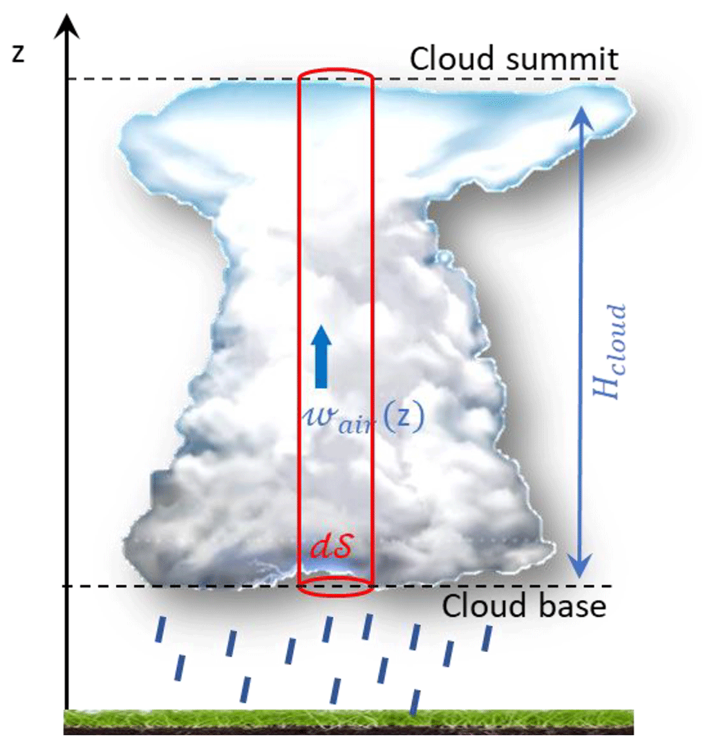
In this elementary cloud volume, it is elementary to calculate the variation in the average mass concentration of aerosols of diameter d_ap in relation to their transfer into precipitation:

$$\begin{array}{}\text{(2)}& \mathrm{d}\mathcal{M}\left(d_{\mathrm{ap}}\right)=-{\displaystyle \frac{{\mathit{\varphi }}_{\mathrm{ap},\mathrm{precip}}\left(d_{\mathrm{ap}}\right)\cdot \mathrm{d}\mathcal{S}\cdot \mathrm{d}t}{\mathrm{d}{V}_{\mathrm{cloud}}}}.\end{array}$$

In this equation, ϕ_ap,precip(d_ap) is the mass flow of dry particles of diameter (d_ap) leaving the cloud via precipitation (solids and liquids) and dV_cloud is the elementary volume of cloud considered ($\mathrm{d}{V}_{\mathrm{cloud}}=H_{\mathrm{cloud}}\cdot \mathrm{d}\mathcal{S}$).

$$\begin{array}{}\text{(3)}& \begin{array}{rl}{\mathrm{\Lambda }}_{\mathrm{cloud}}^m\left(d_{\mathrm{ap}}\right)& =-{\displaystyle \frac{\mathrm{1}}{\mathrm{d}t}}{\displaystyle \frac{\mathrm{d}\mathcal{M}\left(d_{\mathrm{ap}}\right)}{\langle \mathcal{M}\left(d_{\mathrm{ap}}\right)\rangle }}{|}_{\mathrm{cloud}}\\ & ={\displaystyle \frac{{\mathit{\varphi }}_{\mathrm{ap},\mathrm{precip}}\left(d_{\mathrm{ap}}\right){|}_{\mathrm{d}\mathcal{S}}}{\langle \mathcal{M}\left(d_{\mathrm{ap}}\right){\rangle }_{\mathrm{cloud}}\cdot H_{\mathrm{cloud}}}}\end{array}\end{array}$$

In this equation, 〈ℳ(d_ap)〉 is the average mass concentration (over the thickness of the cloud) of dry particles of diameter d_ap. It is noteworthy that 〈ℳ(d_ap)〉 is not the average concentration of interstitial aerosols in the cloud but the average concentration of particles, which includes, in addition to the interstitial aerosols, all the particles included in the droplets and potentially in the ice phase. Thus, if we jointly determine 〈ℳ(d_ap)〉 and ϕ_ap,precip as well as the thickness of the cloud H_cloud, it is possible to deduce a scavenging coefficient.

The average particle concentration is calculated, using Eq. (4), by spatially averaging, over the entire thickness of the cloud, the concentrations of interstitial aerosols (of diameters d_ap) ℳ_int(z,d_ap), the concentrations of particles in the drops (𝕄(z,d_ap)), and the concentrations in the ice phase (𝔐(z,d_ap)).

$$\begin{array}{}\text{(4)}& \begin{array}{rl}\langle \mathcal{M}\left(d_{\mathrm{ap}}\right)\rangle & ={\displaystyle \frac{\mathrm{1}}{H_{\mathrm{cloud}}}}\cdot \underset{\mathrm{cloud}\mathrm{base}}{\overset{\text{cloud summit}}{\int }}\left({\mathcal{M}}_{\mathrm{int}}\right(z,d_{\mathrm{ap}})\\ & +\mathbb{M}(z,d_{\mathrm{ap}})+\mathfrak{M}(z,d_{\mathrm{ap}}))\mathrm{d}z\end{array}\end{array}$$

Finally, in order to evaluate the mass flow of particles exiting the cloud at its base (ϕ_ap,precip(d_ap)), it is necessary to evaluate the cloud volume (𝒱(𝒟_drop)) that contains all the droplets whose drop velocity w_∞(𝒟_drop) is sufficient for them to pass through the section d𝒮 during the time dt. Using the velocity composition law, we can deduce Eq. (5).

$$\begin{array}{}\text{(5)}& \mathcal{V}\left({\mathcal{D}}_{\mathrm{drop}}\right)=max(\mathrm{0},w_{\mathrm{\infty }}({\mathcal{D}}_{\mathrm{drop}})-w_{\mathrm{air}}({\mathcal{Z}}_{\mathrm{cloud}\mathrm{base}}\left)\right)\cdot d\mathcal{S}\end{array}$$

In this equation, w_air(𝒵_cloud base) is the velocity of the air parcel at the base of the cloud. By convention, w_air is positive for an updraught and negative for a downdraught.

It is then immediately possible to deduce the flow of particles passing d𝒮 through liquid precipitation:

$$\begin{array}{}\text{(6)}& \begin{array}{rl}{\mathit{\varphi }}_{\mathrm{ap},\mathrm{rain}}\left(d_{\mathrm{ap}}\right)& ={\int }_{d_{\mathrm{droplet}}=\mathrm{0}}^{\mathrm{\infty }}max(\mathrm{0},w_{\mathrm{\infty }}({\mathcal{D}}_{\mathrm{drop}})\\ & -w_{\mathrm{air}}\left({\mathcal{Z}}_{\mathrm{cloud}\mathrm{base}}\right))\cdot \mathbb{M}(z,d_{\mathrm{ap}},{\mathcal{D}}_{\mathrm{drop}})\cdot \mathrm{d}{\mathcal{D}}_{\mathrm{drop}}.\end{array}\end{array}$$

In this equation, $\mathbb{M}(z,d_{\mathrm{ap}},{\mathcal{D}}_{\mathrm{drop}})$ is the concentration of particles contained in the droplets and of dry diameter d_ap.

The same applies to solid precipitation ϕ_ap,ice(d_ap):

$$\begin{array}{}\text{(7)}& \begin{array}{rl}{\mathit{\varphi }}_{\mathrm{ap},\mathrm{ice}}\left(d_{\mathrm{ap}}\right)& ={\int }_{d_{\mathrm{ice}}=\mathrm{0}}^{\mathrm{\infty }}max(\mathrm{0},w_{\mathrm{\infty }}(d_{\mathrm{ice}})\\ & -w_{\mathrm{air}}\left({\mathcal{Z}}_{\mathrm{cloud}\mathrm{base}}\right))\cdot \mathfrak{M}(z,d_{\mathrm{ap}},d_{\mathrm{ice}})\cdot \mathrm{d}{d}_{\mathrm{ice}}.\end{array}\end{array}$$

By adding these two flows together, it is possible to deduce the total flow of particles (of diameter d_ap) exiting the cloud through all precipitation:

$$\begin{array}{}\text{(8)}& {\mathit{\varphi }}_{\mathrm{ap},\mathrm{precip}}\left(d_{\mathrm{ap}}\right)={\mathit{\varphi }}_{\mathrm{ap},\mathrm{rain}}\left(d_{\mathrm{ap}}\right)+{\mathit{\varphi }}_{\mathrm{ap},\mathrm{ice}}\left(d_{\mathrm{ap}}\right).\end{array}$$

Thus, to theoretically evaluate the cloud scavenging coefficient, it is first and foremost essential to be able to evaluate its contours, but it is also essential to be able to determine the mass concentrations of particles in the droplets $\mathbb{M}(z,d_{\mathrm{ap}},{\mathcal{D}}_{\mathrm{drop}})$, in the ice phase $\mathfrak{M}(z,d_{\mathrm{ice}},d_{\mathrm{ap}})$, and in the interstitial aerosol ℳ_int(z,d_ap).

To evaluate the contours of the cloud, it seems necessary in the first instance to consider once again its definition.

2.2 What is a cloud? (How are its boundaries to be defined?)

The World Meteorological Organization defines clouds as “an aggregation of minute particles of liquid water or ice, or of both, suspended in the atmosphere and usually not touching the ground” (World Meteorological Organization, 2017). This definition would appear to be very inadequate for enabling the contours of a cloud to be determined. Clouds, although very commonly talked about in everyday life and subject to numerous scientific studies, have contours that remain very blurred. It is therefore always difficult to define them rigorously and above all non-recursively. Spänkuch et al. (2022) further emphasised that, depending on the scope of the authors' expertise (meteorology, climate, satellite observations, airborne observations, observations from ground radars, or microphysical models), authors use significantly differing definitions and thresholds.

For example, Wood and Field (2011) proposed criteria with respect to liquid water content (LWC), ice water content (IWC), or total concentrations in the numbers of hydrometeors (droplets and crystals).

Hiron (2017) proposed separating cloud water and precipitation water based on the criterion of the size of hydrometeors (hydrometeors with a diameter of less than 64 µm are considered part of the cloud; hydrometeors larger than that are considered part of the rain); then, if the total cloud water content is greater than 0.1 g cm⁻³, the air parcel is considered part of the cloud.

Other authors have proposed contours based on relative humidity (Del Genio et al., 1996) or total water content (TWC), whereas meteorologists and climatologists tend to prefer optical thickness (Sassen and Cho, 1992), each with arbitrarily established thresholds.

Although these definitions can be linked mathematically to each other, these relationships are most often highly non-linear. Therefore, in this article, a variety of cloud definitions will be considered, and we will examine the criteria that are most relevant for studying in-cloud scavenging and distinguishing it from below-cloud scavenging. The relevance of the definition of what constitutes a cloud will be analysed from two perspectives. We consider, firstly, a purely physical perspective and, secondly, a more pragmatic perspective linked rather to applicability in an atmospheric dispersion model dedicated to crisis management.

2.3 DESCAM

To simulate clouds of different types and theoretically evaluate their scavenging coefficient, it is necessary to have a model that makes it possible to simulate all the water phase changes, considering the catalyst role of aerosols in most of these state changes (activation, ice nucleation, etc.). It is also necessary to calculate the sink terms of interstitial aerosols (related to droplet collection or activation) and associate them with the source terms of particles in droplets and ice in order to calculate the mass of particles in droplets (𝕄(𝒟_drop)) and in ice (𝔐(d_ice)) throughout the simulation (Eqs. 6 and 7).

DESCAM meets these specifications. This detailed microphysical model classifies droplets $({\mathcal{D}}_{\mathrm{drop}}\in [\mathrm{1}\mathrm{\mu }\mathrm{m},\mathrm{6.5}\mathrm{mm}\left]\right)$, ice $(d_{\mathrm{ice}}\in [\mathrm{1}\mathrm{\mu }\mathrm{m},\mathrm{6.5}\mathrm{mm}\left]\right)$, and aerosols $(d_{\mathrm{ap}}\in [\mathrm{2}\mathrm{nm},\mathrm{12.7}\mathrm{\mu }\mathrm{m}\left]\right)$ into 39 logarithmically distributed size classes each. This makes it possible to explicitly monitor their respective particle size distributions, ℕ(𝒟_drop),𝔑(d_ice), and 𝒩(d_ap), spatially and temporally. DESCAM can be coupled with various dynamic models that allow consideration of atmospheric flows. In this article, we will only consider a dynamic called 1D1/2 (Asai and Kasahara, 1967), implemented in DESCAM by Monier et al. (2006). More realistic 3D dynamics (Clark and Hall, 1991) are implemented in DESCAM (Leroy et al., 2007) but will not be considered in this article.

2.3.1 Description of the microphysical models modelled in DESCAM

All the microphysical processes considered in DESCAM are presented in Fig. 2.

Figure 2 Modelling of microphysical processes in DESCAM.

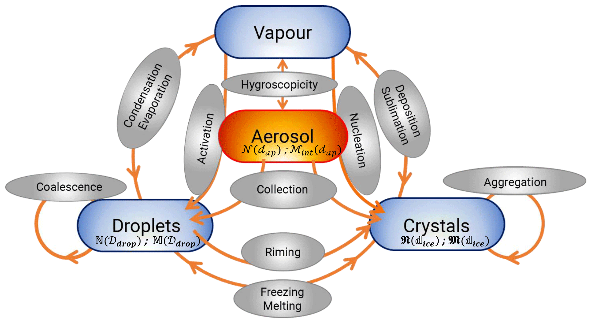
In this figure, we can see the central role of aerosols in most water phase changes. The explicit resolution of all these microprocesses enables calculation of the particle size distributions of aerosols in each grid cell and at each time step (in number 𝒩(d_ap), Eq. 9, and in mass ℳ(d_ap)) as well as the particle size distributions of the droplets (in number ℕ(𝒟_drop), Eq. 10) and of the ice (in number 𝔑(d_ice), Eq. 11). In addition, in order to preserve the total mass of particles, the model also calculates two other quantities that are used to determine the masses of particles in droplets of diameter d_drop (𝕄(𝒟_drop), Eq. 12) and in ice crystals of diameter d_ice (𝔐(d_ice), Eq. 13).

$$\begin{array}{}\text{(9)}& \begin{array}{rl}{\displaystyle \frac{\mathrm{d}\mathcal{N}\left(d_{\mathrm{ap}}\right)}{\mathrm{d}t}}& ={\displaystyle \frac{\mathrm{d}\mathcal{N}\left(d_{\mathrm{ap}}\right)}{\mathrm{d}t}}{|}_{\mathrm{dyn}}+{\displaystyle \frac{\mathrm{d}\mathcal{N}\left(d_{\mathrm{ap}}\right)}{\mathrm{d}t}}{|}_{\mathrm{coll}}\\ & +{\displaystyle \frac{\mathrm{d}\mathcal{N}\left(d_{\mathrm{ap}}\right)}{\mathrm{d}t}}{|}_{\mathrm{hygro}}+{\displaystyle \frac{\mathrm{d}\mathcal{N}\left(d_{\mathrm{ap}}\right)}{\mathrm{d}t}}{|}_{\mathrm{act},\mathrm{deact}}\end{array}\end{array}$$

$$\begin{array}{}\text{(10)}& \begin{array}{rl}{\displaystyle \frac{\mathrm{d}\mathbb{N}\left({\mathcal{D}}_{\mathrm{drop}}\right)}{\mathrm{d}t}}& ={\displaystyle \frac{\mathrm{d}\mathbb{N}\left({\mathcal{D}}_{\mathrm{drop}}\right)}{\mathrm{d}t}}{|}_{\mathrm{dyn}}+{\displaystyle \frac{\mathrm{d}\mathbb{N}\left({\mathcal{D}}_{\mathrm{drop}}\right)}{\mathrm{d}t}}{|}_{\mathrm{act},\mathrm{deact}}\\ & +{\displaystyle \frac{\mathrm{d}\mathbb{N}\left({\mathcal{D}}_{\mathrm{drop}}\right)}{\mathrm{d}t}}{|}_{\mathrm{coal}}+{\displaystyle \frac{\mathrm{d}\mathbb{N}\left({\mathcal{D}}_{\mathrm{drop}}\right)}{\mathrm{d}t}}{|}_{\mathrm{cond},\mathrm{vap}}\\ & +{\displaystyle \frac{\mathrm{d}\mathbb{N}\left({\mathcal{D}}_{\mathrm{drop}}\right)}{\mathrm{d}t}}{|}_{\mathrm{riming}}+{\displaystyle \frac{\mathrm{d}\mathbb{N}\left({\mathcal{D}}_{\mathrm{drop}}\right)}{\mathrm{d}t}}{|}_{\mathrm{frz},\mathrm{melt}}\end{array}\end{array}$$

$$\begin{array}{}\text{(11)}& \begin{array}{rl}{\displaystyle \frac{\mathrm{d}\mathfrak{N}\left(d_{\mathrm{ice}}\right)}{\mathrm{d}t}}& ={\displaystyle \frac{\mathrm{d}\mathfrak{N}\left(d_{\mathrm{ice}}\right)}{\mathrm{d}t}}{|}_{\mathrm{dyn}}+{\displaystyle \frac{\mathrm{d}\mathfrak{N}\left(d_{\mathrm{ice}}\right)}{\mathrm{d}t}}{|}_{\mathrm{nucleation}}\\ & +{\displaystyle \frac{\mathrm{d}\mathfrak{N}\left(d_{\mathrm{ice}}\right)}{\mathrm{d}t}}{|}_{\mathrm{frz},\mathrm{sub}}+{\displaystyle \frac{\mathrm{d}\mathfrak{N}\left(d_{\mathrm{ice}}\right)}{\mathrm{d}t}}{|}_{\mathrm{agg}}\\ & +{\displaystyle \frac{\mathrm{d}\mathfrak{N}\left(d_{\mathrm{ice}}\right)}{\mathrm{d}t}}{|}_{\mathrm{riming}}+{\displaystyle \frac{\mathrm{d}\mathbb{N}\left(d_{\mathrm{ice}}\right)}{\mathrm{d}t}}{|}_{\mathrm{frz},\mathrm{melt}}\end{array}\end{array}$$

$$\begin{array}{}\text{(12)}& \begin{array}{rl}{\displaystyle \frac{\mathrm{d}\mathbb{M}\left({\mathcal{D}}_{\mathrm{drop}}\right)}{\mathrm{d}t}}& ={\displaystyle \frac{\mathrm{d}\mathbb{M}\left({\mathcal{D}}_{\mathrm{drop}}\right)}{\mathrm{d}t}}{|}_{\mathrm{dyn}}+{\displaystyle \frac{\mathrm{d}\mathbb{M}\left({\mathcal{D}}_{\mathrm{drop}}\right)}{\mathrm{d}t}}{|}_{\mathrm{act},\mathrm{deact}}\\ & +{\displaystyle \frac{\mathrm{d}\mathbb{M}\left({\mathcal{D}}_{\mathrm{drop}}\right)}{\mathrm{d}t}}{|}_{\mathrm{coal}}+{\displaystyle \frac{\mathrm{d}\mathbb{M}\left({\mathcal{D}}_{\mathrm{drop}}\right)}{\mathrm{d}t}}{|}_{\mathrm{cond},\mathrm{vap}}\\ & +{\displaystyle \frac{\mathrm{d}\mathbb{M}\left({\mathcal{D}}_{\mathrm{drop}}\right)}{\mathrm{d}t}}{|}_{\mathrm{riming}}+{\displaystyle \frac{\mathrm{d}\mathbb{M}\left({\mathcal{D}}_{\mathrm{drop}}\right)}{\mathrm{d}t}}{|}_{\mathrm{frz},\mathrm{melt}}\end{array}\end{array}$$

$$\begin{array}{}\text{(13)}& \begin{array}{rl}{\displaystyle \frac{\mathrm{d}\mathfrak{M}\left(d_{\mathrm{ice}}\right)}{\mathrm{d}t}}& ={\displaystyle \frac{\mathrm{d}\mathfrak{M}\left(d_{\mathrm{ice}}\right)}{\mathrm{d}t}}{|}_{\mathrm{dyn}}+{\displaystyle \frac{\mathrm{d}\mathfrak{M}\left(d_{\mathrm{ice}}\right)}{\mathrm{d}t}}{|}_{\mathrm{nucleation}}\\ & +{\displaystyle \frac{\mathrm{d}\mathfrak{M}\left(d_{\mathrm{ice}}\right)}{\mathrm{d}t}}{|}_{\mathrm{frz},\mathrm{sub}}+{\displaystyle \frac{\mathrm{d}\mathfrak{M}\left(d_{\mathrm{ice}}\right)}{\mathrm{d}t}}{|}_{\mathrm{aggg}}\\ & +{\displaystyle \frac{\mathrm{d}\mathfrak{M}\left(d_{\mathrm{ice}}\right)}{\mathrm{d}t}}{|}_{\mathrm{riming}}+{\displaystyle \frac{\mathrm{d}\mathfrak{M}\left(d_{\mathrm{ice}}\right)}{\mathrm{d}t}}{|}_{\mathrm{frz},\mathrm{melt}}\end{array}\end{array}$$

In these equations, except for the index ( |_dyn) denoting variations due to atmospheric transport, each term corresponds to one of the microphysical processes outlined in Fig. 2. For instance, $\left({|}_{\mathrm{act},\mathrm{deact}}\right)$ denotes activation and deactivation processes. The subscripts coll, hygro, frz, sub, coal, cond, vap, and agg refer to the processes of aerosol collection by droplets, hygroscopicity of aerosol particles, freezing, sublimation, coalescence, condensation, vaporisation, and aggregation, respectively. The hygroscopic growth of aerosol particles is calculated assuming that they are in thermodynamic equilibrium with the air supersaturation S (Eq. 14). This equilibrium is modelled after κ-Köhler theory.

$$\begin{array}{}\text{(14)}& {\displaystyle \frac{\mathrm{d}\mathcal{N}\left(d_{\mathrm{ap}}\right)}{\mathrm{d}t}}{|}_{\mathrm{hygro}}={\displaystyle \frac{\partial \mathcal{N}\left(d_{\mathrm{ap}}\right)}{\partial \mathcal{S}}}{|}_{\mathit{\kappa }\text{-Köhler}}{\displaystyle \frac{\partial \mathcal{S}}{\partial t}}{|}_{\mathrm{dyn}}\end{array}$$

Concerning the cold microphysics (Fig. 2), this simulation integrates homogeneous freezing mechanisms (i.e. which do not require aerosol contribution) and heterogeneous freezing mechanisms (for which aerosols act as a catalyst for phase change). For homogeneous freezing, we consider the parameterisation of Koop et al. (2000) adapted to DESCAM by Monier et al. (2006). To model heterogeneous ice nucleation, we consider all the mechanisms described by Vali et al. (2015). The Bigg (1953) formula is used to describe immersion freezing, and the model of Meyers et al. (1992) is used for condensation and contact freezing, as well as deposition nucleation. All these mechanisms have recently been incorporated into DESCAM by Hiron and Flossmann (2015).

The main mechanism responsible for the flow of particles exiting the cloud via precipitation (ϕ_ap,precip(d_ap), Eq. 3) is activation. The collection of aerosols by droplets is only second order (Dépée et al., 2019; Flossmann and Wobrock, 2010). In DESCAM, activation is modelled by κ-Köhler theory (Petters and Kreidenweis, 2007). This model makes it possible to determine equilibrium vapour pressure in the vicinity of a droplet of diameter 𝒟_drop, as a function of the mass and type of solute (modelled by the κ value) it contains, and therefore the supersaturation for this droplet. For a given mass and chemical nature of the pristine dry particle, one can compute the corresponding supersaturations for a given size of solution droplets. This curve has a unique maximum, called critical supersaturation (Fig. 3). The diameter associated with this critical supersaturation is called the activation diameter. Aerosols with a diameter smaller than the activation diameter are brought into thermodynamic equilibrium with their environment by hygroscopicity, with aerosols of a diameter greater than the activation diameter being converted into droplets and growing by means of vapour diffusion (by condensation).

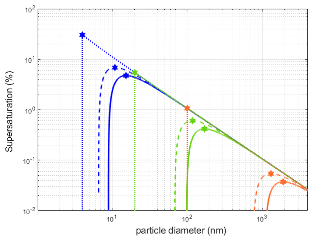
Figure 3 Thermodynamic equilibrium of an aerosol calculated as a function of the particle diameter and nature of the initial dry particle. This calculation is made using κ-Köhler theory (for a temperature of 293 K and a surface tension between solution and air of 72 × 10⁻³ N m⁻¹). Line colours denote the following: blue (), initial dry radius of the particles set at 4 nm; green (), initial dry radius set at 20 nm; and orange (), initial dry radius set at 100 nm. Line styles denote the following: dotted, κ=0, insoluble aerosol; dashed, κ=0.61, moderately hygroscopic, as (NH₄)₂SO₄; and solid, κ=1.28, highly hygroscopic, as NaCl. The star markers () denote critical supersaturations needed to activate the aerosol and convert it into a cloud droplet.

In the DESCAM code, the microphysical process of collection (i.e. the process by which, during falling, droplets encounter impact and capture interstitial aerosol particles) is modelled in Eq. (12) by the term $\frac{\mathrm{d}\mathbb{M}\left({\mathcal{D}}_{\mathrm{drop}}\right)}{\mathrm{d}t}{|}_{\mathrm{coll}}$, which is calculated by solving Eq. (15). In this equation, the central term is the collection efficiencies $\left(E\right(d_{\mathrm{ap}},{\mathcal{D}}_{\mathrm{drop}},\text{RH}\left)\right)$. This is calculated by the model developed and validated by Dépée et al. (2019, 2021a, b).

$$\begin{array}{}\text{(15)}& \begin{array}{rl}{\displaystyle \frac{\mathrm{d}\mathbb{M}\left({\mathcal{D}}_{\mathrm{drop}}\right)}{\mathrm{d}t}}{|}_{\mathrm{coll}}& ={\int }_{d_{\mathrm{ap}}=\mathrm{0}}^{\mathrm{\infty }}\mathcal{N}\left(d_{\mathrm{ap}}\right){\displaystyle \frac{\mathit{\pi }{\mathcal{D}}_{\mathrm{drop}}^{\mathrm{2}}}{\mathrm{4}}}{\mathcal{U}}_{\mathrm{\infty },\mathrm{droplet}}\left({\mathcal{D}}_{\mathrm{drop}}\right)\\ & \cdot E(d_{\mathrm{ap}},{\mathcal{D}}_{\mathrm{drop}},\text{RH}){\displaystyle \frac{\mathit{\pi }{d}_{\mathrm{ap}}^{\mathrm{3}}}{\mathrm{6}}}{\mathit{\rho }}_{\mathrm{ap}}\mathrm{d}{d}_{\mathrm{ap}}\end{array}\end{array}$$

In this equation 𝒰_∞,droplet(𝒟_drop) corresponds to the terminal velocity of a droplet of diameter 𝒟_drop (calculated after the Beard, 1974, model), ρ_ap is the density of the aerosol particle, and RH refers to the relative humidity of air in the parcel.

Note that Eqs. (6) and (7) are not directly calculable by DESCAM. This is because the model makes an inventory of the mass of particles in the droplets and crystals according to the size of the hydrometeors (𝕄(𝒟_drop), Eq. 12, and 𝔐(d_ice), Eq. 13) but without memorising the size of the aerosols before their incorporation. The scavenging coefficients calculated in this article are therefore averaged, in mass, over the particle size distribution of the aerosols. In this article we focus on validating the approach described by applying it to different types of clouds. Current work and future publications will focus on demonstrating that the scavenging coefficient may be simply spectrally calculated, without modifying the model.

2.3.2 Modelling of atmospheric dynamics

As stated previously, in this article we have limited our study to the 1.5D dynamic framework developed by Asai and Kasahara (1967). This has been regularly used (Hiron and Flossmann, 2015; Leroy et al., 2007; Monier et al., 2006; Quérel et al., 2014) to study the microphysical processes involved in the life cycle of cumulus clouds. This model considers two concentric cylinders. The inner cylinder has a radius 10 times smaller than the outer cylinder. In the inner cylinder, the vertical velocity of the flows is determined by solving a simplified form of the Navier–Stokes equations, coupled with the energy conservation equation. The outer cylinder serves primarily to guarantee the condition of zero velocity divergence (continuity equation for incompressible flow). To this end, a radial velocity component is introduced at the interface between these two cylinders (hence the expression of a 1.5D model), calculated from the convergence or divergence layers and allowing entrainment from the environment. In this environment the only variable updated in this outer cylinder is the vertical velocity to evaluate the radial gradient in vertical velocity and the subsequent turbulent flux; all the other variables are assumed to be unaffected by the cloud processes within the inner cylinder and are kept constant throughout the simulation.

All the microphysical processes detailed in the previous section and summarised in Fig. 2 are calculated only in the central cylinder. Thus, it is also in the inner cylinder, for each grid layer, that phase changes in the water are computed, with the subsequent absorption or release of latent heat that alters the buoyancy of the air and which ultimately generates the updraught and downdraught motions.

3 Application to example cloud types

To establish a theoretical scavenging coefficient scheme, the methodology described above is applied to two very different idealised case studies representative of two different cloud types. First, we will model a vigorous cumulonimbus and then a shallow stratus. These two cloud types were selected as they present the higher and lower values, respectively, in terms of vertical extension, relative humidity, and rainfall intensity. Furthermore, while the stratus that we simulate is shallow enough to be a warm cloud, cold microphysical processes are essential to capture the development of the cumulonimbus situation.

3.1 Application to a cumulonimbus

3.1.1 Description of the cumulonimbus considered

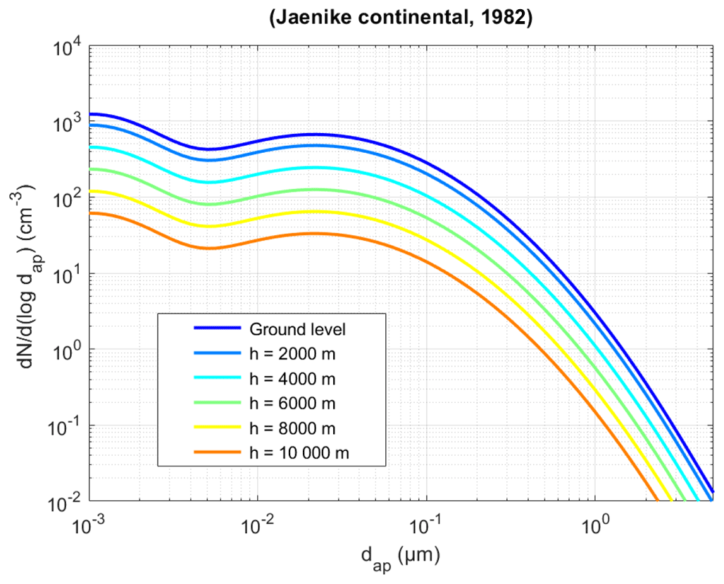
The cloud selected to model the cumulonimbus is from the episode of 19 July 1981 of the CCOPE campaign (Dye et al., 1986; Knight, 1982), which took place near Miles City in Montana (USA). This episode was selected because it is very finely documented and is a test case for many codes simulating the formation of convective clouds, in particular DESCAM (Flossmann and Wobrock, 2010). A radio sounding taken at Miles City at 16:00 LT (just before the storm) is used to initialise the thermodynamic conditions of the atmospheric column: temperature and humidity. For the vertical pressure profiles, standard conditions are assumed. In addition, we used the observations of two Doppler radars measuring high-resolution reflectivity as well as the movements of the cloud and five aircraft that were able to make numerous passes through the cloud throughout its maturation and through to the precipitation episodes. The spatial–temporal evolution of the thermodynamic conditions, associated with the microphysical properties of the cloud system, and the atmospheric flows are therefore recorded in fine detail for the entire life of this cumulonimbus and can be used to evaluate the model performance to capture the clouds physics. For this article, we therefore used the same modelling hypotheses as those detailed by Leroy et al. (2006). Convection was triggered by +2.3 °C heating of the ground during the first 10 min of the simulation. During this campaign, no physicochemical measurements were made of the aerosols; hence we assume they consisted of ammonium sulfate (κ = 0.61 and ρ_dry = 1.77×10³ kg m⁻³; Petters and Kreidenweis, 2007) with an initial particle size distribution of the Jaenicke (1982) continental type. We assumed a homogeneous distribution in the atmospheric boundary layer (i.e. over the first 3 km); then above the concentration is assumed to decrease exponentially with a scale height of 3000 m (Fig. 4).

Figure 4 Initial particle size distribution of aerosols considered for this simulation.

The simulation lasted 3600 s on a 10 km high column. The spatial and temporal resolutions were set to 100 m and 3 s, respectively.

Figures 5 and 6 show the spatial–temporal evolutions of the vertical flows in the central cylinder and the liquid water and ice content, respectively.

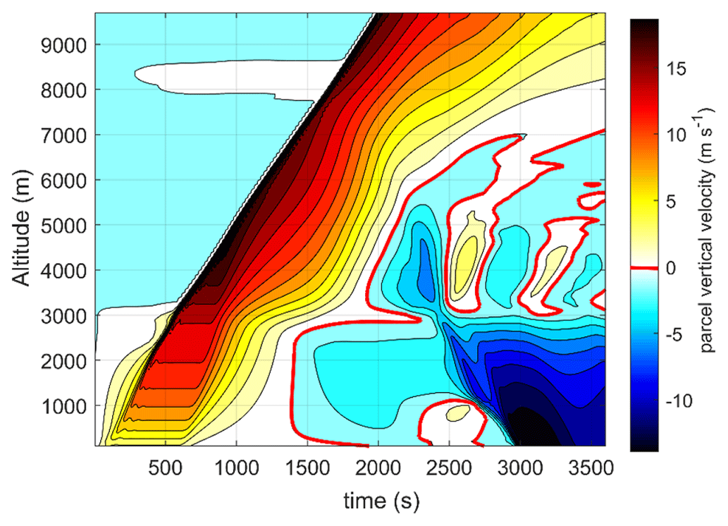
Figure 5 Spatial–temporal distribution of the vertical components of atmospheric flows. The thick line in red separates the updraught (w_air > 0) flows from the downdraught flows (w_air <0).

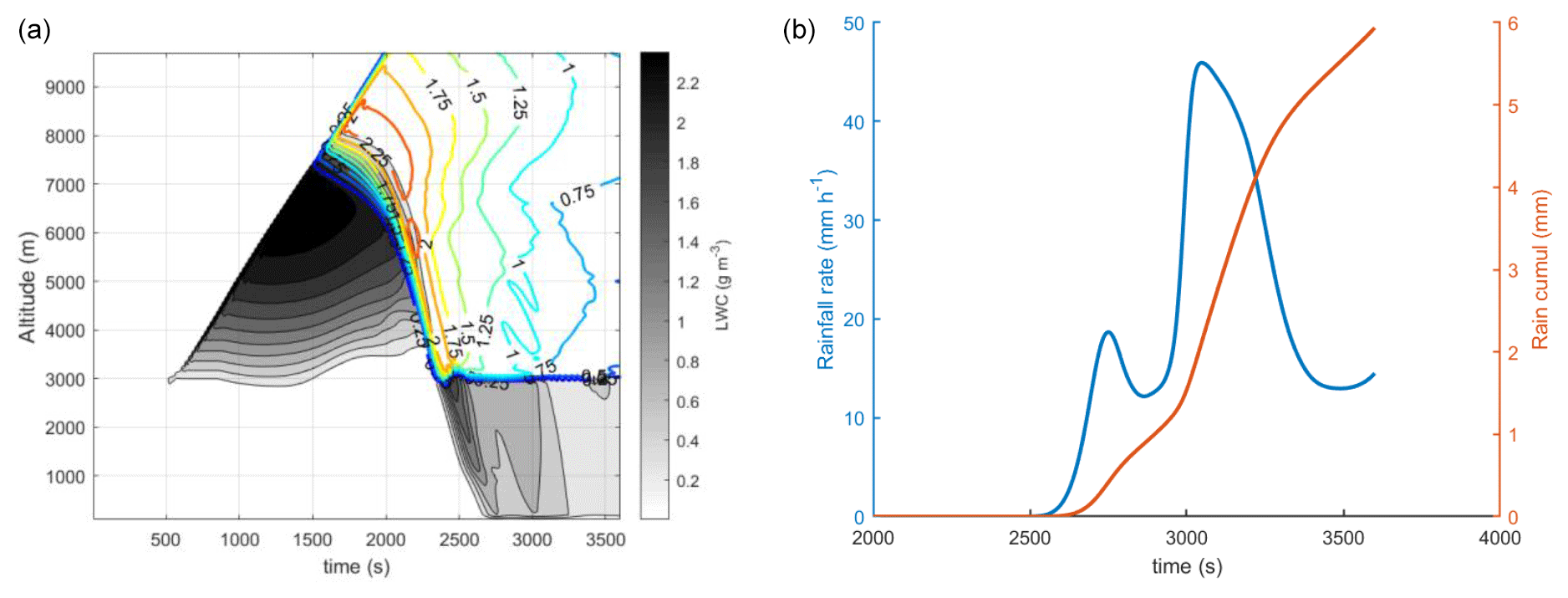
Figure 6 (a) Spatial–temporal distributions of liquid water content (LWC, greyscale) and ice water content (IWC, iso-contours). (b) Temporal evolution of rainfall intensity and cumulative precipitation at ground level.

In these figures, we can see that the initial superheating of the air layer at ground level induces an updraught flow due to buoyancy forces. Approximately 500 s after the start of the simulation, the air reaches critical supersaturation at an altitude of 3000 m and the aerosols are gradually converted into droplets. The spatial–temporal distribution shown on the left of Fig. 6 highlights the appearance of a cloud at the spatial–temporal coordinate (500 s, 3000 m). Vapour condensation induces a latent heat release, which in turn increases buoyancy of the air parcel and accelerates the updraught flows (approx. 15 m s⁻¹ at 4000 m). This flow transports the vapour at altitude, and by cooling this induces the progressive activation of the aerosols and a vertical extension of the cloud. Near 7000 m, the first ice crystals are formed. The coexistence of ice crystals and supercooled droplets allows rapid crystal growth with a corresponding reduction in liquid water content (best known as the WBF process, which is derived from Wegener, 1911; Bergeron, 1928; and Findeisen, 1938). Then, the crystals begin to precipitate at around 1700 s, since they reach sizes large enough for their gravitational settling velocity to supersede updraught speed. In precipitating, the larger crystals collect the suspended droplets. Hence, under the coupled influence of the WBF process and, above all, the collection of droplets by the ice particles, after 2200 s of simulation the cloud only contains ice. Finally, below an altitude of 3000 m, the solid hydrometeors melt and liquid precipitation forms. Figure 6 shows the rainfall intensities on the right, as well as the cumulative precipitation calculated by the model at ground level. This timeline presents two local maxima: the first at 2750 s after the start of the simulation, corresponding to an intensity of 18 mm h⁻¹, and the second 300 s later, with an intensity of about 46 mm h⁻¹.

3.1.2 Calculation of the scavenging coefficient

Based on the modelling results, we applied the methodology described in Sect. 2.1. The first step was to establish the contours of the cloud, then to use Eq. (3) integrated over the entire aerosol distribution, and finally to calculate the cloud's equivalent trapping coefficient.

$$\begin{array}{}\text{(16)}& {\mathrm{\Lambda }}_{\mathrm{cloud}}^m=-{\displaystyle \frac{\mathrm{1}}{\mathrm{d}t}}{\displaystyle \frac{\mathrm{d}\mathcal{M}}{\langle \mathcal{M}\rangle }}{|}_{\mathrm{cloud}}={\displaystyle \frac{{\mathit{\varphi }}_{\mathrm{ap},\mathrm{precip}}}{\langle \mathcal{M}\rangle \cdot H_{\mathrm{cloud}}}}\end{array}$$

As already indicated in Sect. 2.2, there is no strict definition of the boundaries of the cloud, particularly at the interface with the precipitation, and it can also be observed in Fig. 6 that the total water content does not show any demarcation between the cloud and the precipitation. Moreover, as Spänkuch et al. (2022) point out, the physical phenomenon studied will determine which contours are the most relevant. Therefore, for this study, we examined three of the physical parameters to establish this contour. These three criteria are the relative humidity of the air parcel (calculated in relation to liquid water); the mass concentration of hydrometeors with a diameter of less than 64 µm; and, lastly, the concentration of hydrometeors. The contours of this cumulonimbus are presented in Fig. 7 for each of these criteria, each with two thresholds considered. The thresholds levels were chosen arbitrarily, mainly to observe their influence on scavenging when they vary over wide ranges of values.

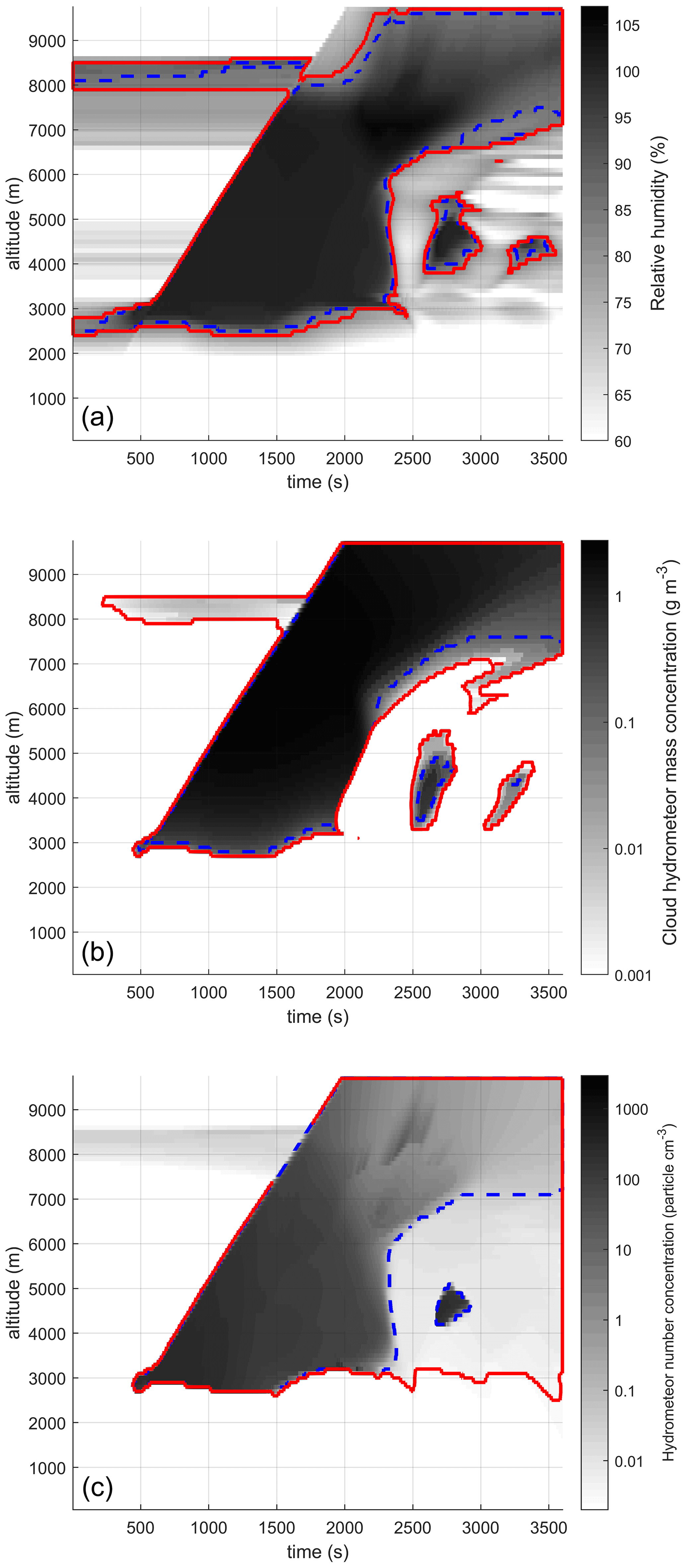
Figure 7 Test of different criteria and thresholds to establish the contours of the simulated cumulonimbus. (a) Threshold based on relative humidity: () RH > 85 % and () RH > 80 %. (b) Threshold based on the total water content of hydrometeors with a diameter less than 64 µm: () mass concentration of cloud hydrometeors > 0.1 g m⁻³ and () mass concentration of cloud hydrometeors > 0.001 g m⁻³. (c) Threshold based on number concentration of total hydrometeors: () $\int \mathrm{d}\mathbb{N}+\mathrm{d}\mathfrak{N}$ > 0.03 cm⁻³ and () $\int \mathrm{d}\mathbb{N}+\mathrm{d}\mathfrak{N}$ > 0.003 cm⁻³.

We can see in this figure that, apart from the criterion based on the concentration of hydrometeors (Eq. 9), with a threshold of 0.003 hydrometeors cm⁻³, the five contours yield very similar clouds. Thus, the cloud forms close to an altitude of 3000 m and its base remains constant for up to 2500 s of simulation. During this 2500 s, the cloud thickens vertically until it reaches the tropopause (considered to be at 10 000 m in this calculation). As shown in Fig. 6b, 2500 s corresponds to the start of precipitation. This moment corresponds to an elevation of the base of the cloud up to about 7000 m, except for the last criterion (𝒩_hydrometeor > 0.003 cm⁻³), for which the height of the base of the cloud remains constant close to the altitude of 3000 m, even during rain.

Initially, our objective was to find a bijective relationship between a set of meteorological parameters available in DESCAM and the scavenging coefficient calculated by this methodology. The reason for a bijective relationship is twofold: first it ensures a better robustness of the model, and second it allows for the performance of inverse calculation to estimate the discharge in the case of ground contamination.

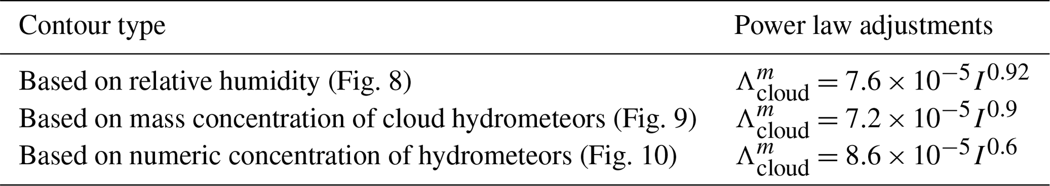
Most often in the literature, cloud scavenging is described as a power function of precipitation intensity (Groëll et al., 2014; Hertel et al., 1995; Leadbetter et al., 2015; Saito et al., 2015b; Quérel et al., 2021). Figures 8–10 present the contours of the cloud established on the basis of the three criteria previously introduced (Fig. 7). Within these contours, we calculated the total mass concentration of ammonium sulfate (ℳ(z)), adding together the respective concentrations of the aerosol phases (ℳ_int(z)) in the droplets (𝕄(z)) and in the crystals (𝔐(z)). Knowing the flux of ammonium sulfate that is within the precipitative hydrometeors through the base of the cloud (Eqs. 6–8), we could deduce the scavenging coefficient, which we plotted according to the precipitation intensity calculated at the base of the cloud. Like in Costa et al. (2010), Stephan et al. (2008), and Quérel et al. (2021), a threshold of 0.1 mm h⁻¹ was considered to limit noise. In Figs. 8–10, the correspondence of the dots can be deduced with the colour codes of the points. On the left-hand side, the identification of the spatial–temporal coordinates where precipitation and the scavenging coefficient are calculated is plotted. On the right-hand side, the corresponding relationship between the scavenging coefficient and precipitation intensity can be read. These results are of great importance because they show that the relationship between the scavenging coefficient and the rainfall intensity is the same at the beginning and the end of the rainfall episode. In addition, an adjustment by a power law is determined for each contour. The coefficients for these adjustments are shown in Table 1.

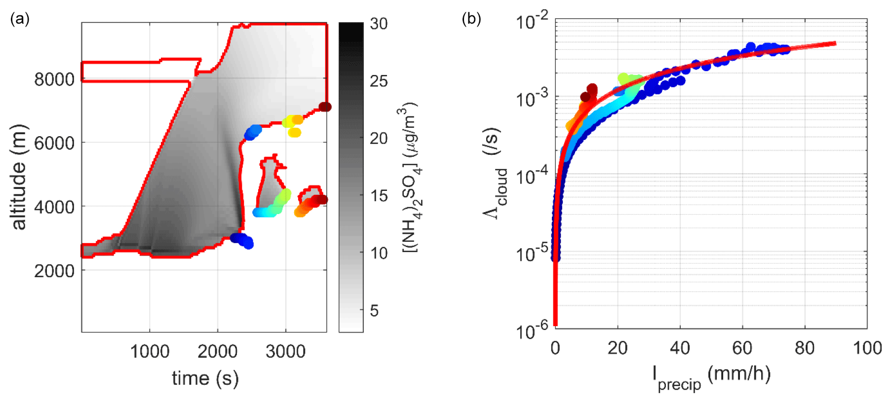
Figure 8 (a) Spatial–temporal distribution of the ammonium sulfate concentration in the cloud contour (the solid line shows the cloud contour for a relative humidity greater than 80 %). (b) Correlation between the scavenging coefficient and the precipitation intensity determined at the base of the cloud, adjusted by a power law (solid line).

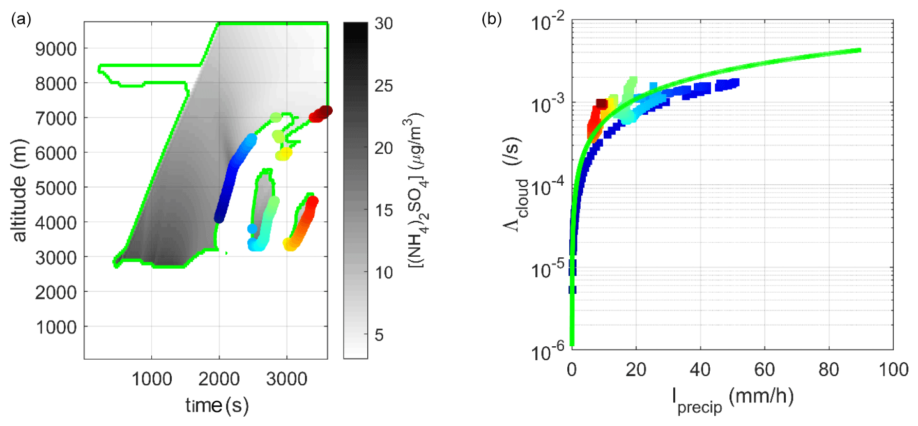
Figure 9 (a) Spatial–temporal distribution of the ammonium sulfate concentration in the cloud contour (the solid line shows the cloud contour for a mass concentration of cloud hydrometeors greater than 0.001 g m⁻³). (b) Correlation between the scavenging coefficient and the precipitation intensity determined at the base of the cloud, adjusted by a power law (solid line).

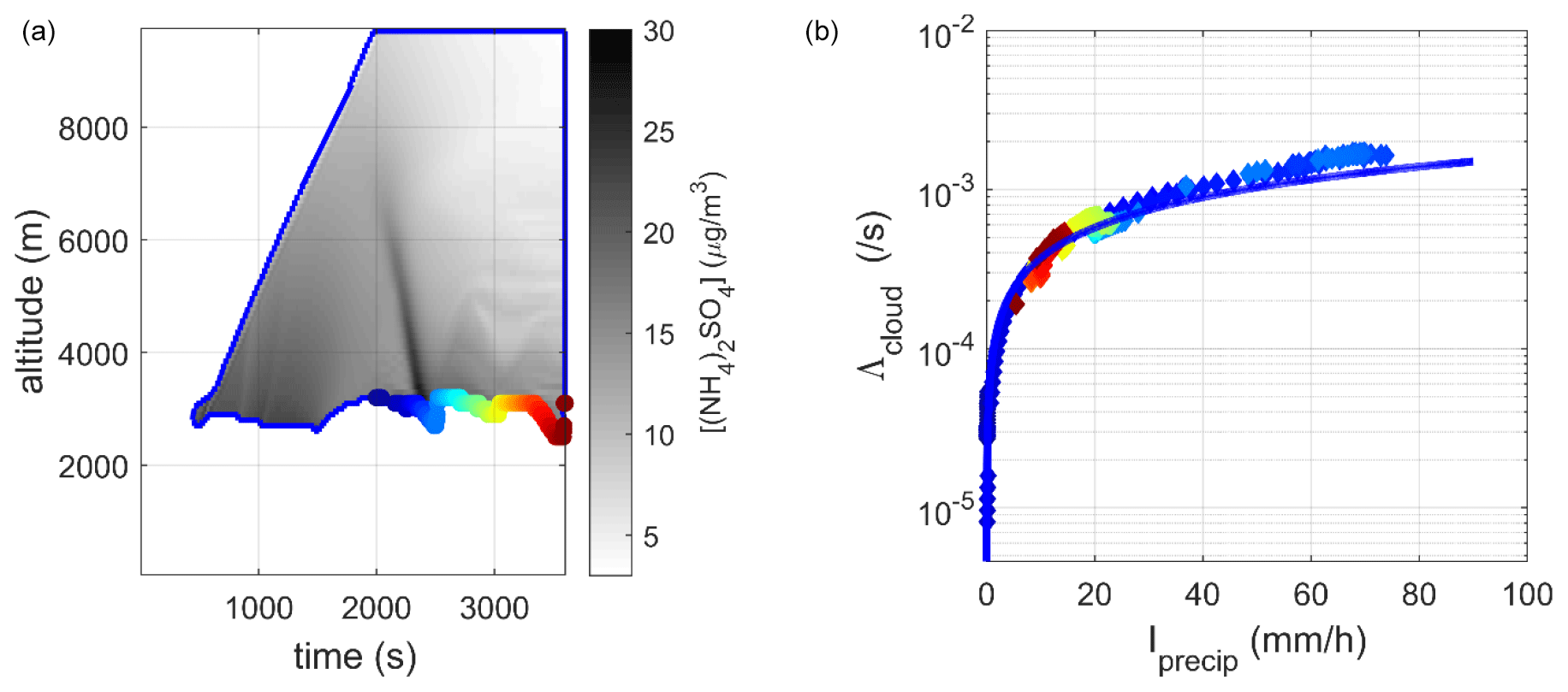
Figure 10 (a) Spatial–temporal distribution of the ammonium sulfate concentration in the cloud contour (the solid line shows the cloud contour for a concentration in the number of hydrometeors greater than 0.003 particles cm⁻³). (b) Correlation between the scavenging coefficient and the precipitation intensity determined at the base of the cloud, adjusted by a power law (solid line).

Table 1 Power law adjustment associated with each of the cloud contours studied.

In these three figures, we observe that the relationship linking the intensity of precipitation to the scavenging coefficient by the cloud is fairly insensitive to the definition selected to describe its contour. Moreover, the power law adjustments plotted in Figs. 8–10 are very similar (Table 1). Nevertheless, only the last contour, based on the hydrometeor concentration (and with a threshold of 0.003 cm⁻³), gives a perfectly bijective relationship between the precipitation intensity at the base of the defined contour and the scavenging coefficient. This result is surprising because, as previously mentioned in Sect. 2.3, the driving mechanism for in-cloud scavenging is dominated by the activation – which is driven by the supersaturation level and physical–chemical properties of the aerosols (Flossmann and Wobrock, 2010). It would therefore seem logical that a criterion based on the relative humidity in the grid cell would be the most relevant. However, it is the criterion based on the concentration of hydrometeors that is the more reliable. This is because there are zones in the cloud where the humidity is too low to activate the aerosols (e.g. at 4000 m at 2500 s where RH < 85 %, as seen in Fig. 7a) but where there is a significant number of droplets and crystals (> 0.03 cm⁻³). These droplets and crystals have been activated elsewhere and previously, but they nevertheless continue to collect aerosols around them – for example by Brownian capture – contributing to scavenging. It is therefore justifiable to define a cloud contour based on a diagnostic of the numeric concentration of hydrometeors.

However, this numeric-concentration criterion, although more precise for theoretically assessing the scavenging coefficient, is not easily accessible in a crisis code. Nevertheless, detailed analysis of the results of these simulations seems to show that it would be wise to define the cloud base as being constant and equal to the altitude at which critical supersaturation is first reached, i.e. the altitude at which the cloud begins its formation.

3.2 Application to a stratus

3.2.1 Description of the stratus considered

The same approach as above was considered for modelling scavenging by a shallow stratus cloud. The main difference with the previous modelling (i.e. with the cumulonimbus) beyond the initialisation of the thermodynamical profile is the treatment of the vertical advection within the cloud. Whereas, for the previous modelling, differences in air buoyancy (related to the initial thermal gradients and latent heat released by water phase changes) were the cause of vertical velocities and could be described and captured by the dynamics of the model, when it comes to modelling stratus clouds, the dynamics are governed by large-scale features that are not included in the 1.5D model. Therefore, the idea is to completely prescribe the time-evolving profile for vertical velocity to model this forcing. Since convection is forced rather than triggered by buoyancy, it is reasonable to prescribe it and not calculate the microphysical feedback on dynamics. For the scenario, we considered the vertical advection model proposed by Zhang et al. (2004) and recapitulated in Eq. (16). We therefore imposed a sinusoidal-profile vertical velocity, with the maximum oscillating from positive to negative values with a period of 1800 s. The maximum of the velocities was located at the altitude (z_c) of 1000 m, and vertical motions were allowed between 700 and 1300 m (h_c = 600 m; Fig. 11). Like Zhang et al. (2004), in the advection model, we imposed an average updraught velocity (w₀) of 0.2 m s⁻¹ and an oscillation amplitude (w₁) of 0.8 m s⁻¹ at an altitude of 1000 m. Figure 5 shows the spatial–temporal distribution of vertical flows prescribed in the central cylinder. The temperature profile follows a dry adiabatic lapse rate with a temperature of 15 °C on the ground so that there are no negative temperatures in the cloud. Above 1300 m, like Zhang et al. (2004), we imposed an inversion of the thermal profile. At altitudes between 700 and 1300 m, the relative humidity was initialised at 98.5 %, and it was 95 % outside of this range. For the aerosols, the initial conditions were identical to those for cumulonimbus (Eq. 5).

$$\begin{array}{}\text{(17)}& \left\{\begin{array}{l}\begin{array}{rl}& w(z,t)=\cos \left(\mathit{\pi }{\displaystyle \frac{z-z_{\mathrm{c}}}{h_{\mathrm{c}}}}\right)\left[w_{\mathrm{0}}+w_{\mathrm{1}}\sin \left({\displaystyle \frac{\mathrm{2}\mathit{\pi }t}{t_{\mathrm{c}}}}\right)\right]\\ & \text{if}|z-z_{\mathrm{c}}|\le {\displaystyle \frac{h_{\mathrm{c}}}{\mathrm{2}}}\end{array}\\ \\ w(z,t)=\mathrm{0}\text{if}|z-z_{\mathrm{c}}|>\frac{h_{\mathrm{c}}}{\mathrm{2}}\\ \\ z_{\mathrm{c}}=\mathrm{1000}\mathrm{m};h_{\mathrm{c}}=\mathrm{600}\mathrm{m};t_{\mathrm{c}}=\mathrm{1800}\mathrm{s};\\ w_{\mathrm{0}}=\mathrm{0.2}\mathrm{m}{\mathrm{s}}^{-\mathrm{1}};w_{\mathrm{1}}=\mathrm{0.8}\mathrm{m}{\mathrm{s}}^{-\mathrm{1}}\end{array}\right.\end{array}$$

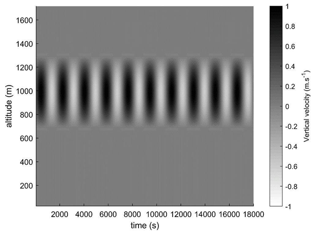
Figure 11 Spatial–temporal distribution of the vertical components of atmospheric flows (Zhang et al., 2004).

Figure 12 shows on the left the spatial–temporal distribution of the water content calculated by DESCAM. The critical supersaturation was reached close to the altitude of 700 m from the first updraught phase (0–1000 s). The LWC then increased with altitude throughout the phase when the atmospheric flows were ascending. At the cloud summit, the liquid water content reached approximately 1.6 g m⁻³. Conversely, during the downdraught phases, the supply of dry air to lower altitudes induced, due to the temperature profile considered, a drop in the relative humidity, which in turn induced evaporation of the droplets and resulted in a significant reduction in the LWC. These downdraught phases also had the effect of advecting droplets below the cloud band. During the period of velocity oscillations (t<t_c), precipitation completely evaporated before reaching the ground. However, from the second period onwards, rain was diagnosed at ground level (Fig. 6b).

Figure 12 (a) Spatial–temporal distribution of the liquid water content calculated by DESCAM (LWC, in greyscale). (b) Temporal evolution of rainfall intensity and cumulative precipitation diagnosed by DESCAM at ground level.

DESCAM predicts intermittent precipitation at ground level with flurries of precipitation on the order of 1 mm h⁻¹. Over a precipitation period of approximately 4 h, the cumulative precipitation was only approximately 3 mm.

3.2.2 Calculation of the stratus scavenging coefficient

As before in the case of cumulonimbus, it is necessary to define the contours of the cloud. We therefore used the three criteria previously introduced and look for the one with the clearest demarcation line between the cloud zone and the precipitation zone to apply a dedicated scavenging coefficient (Fig. 13). As before, we observe from Fig. 12a that water content is not a good indicator for outlining the cloud boundaries. Indeed, no discontinuity is observed for this parameter that would enable demarcation between the cloud and the precipitation.

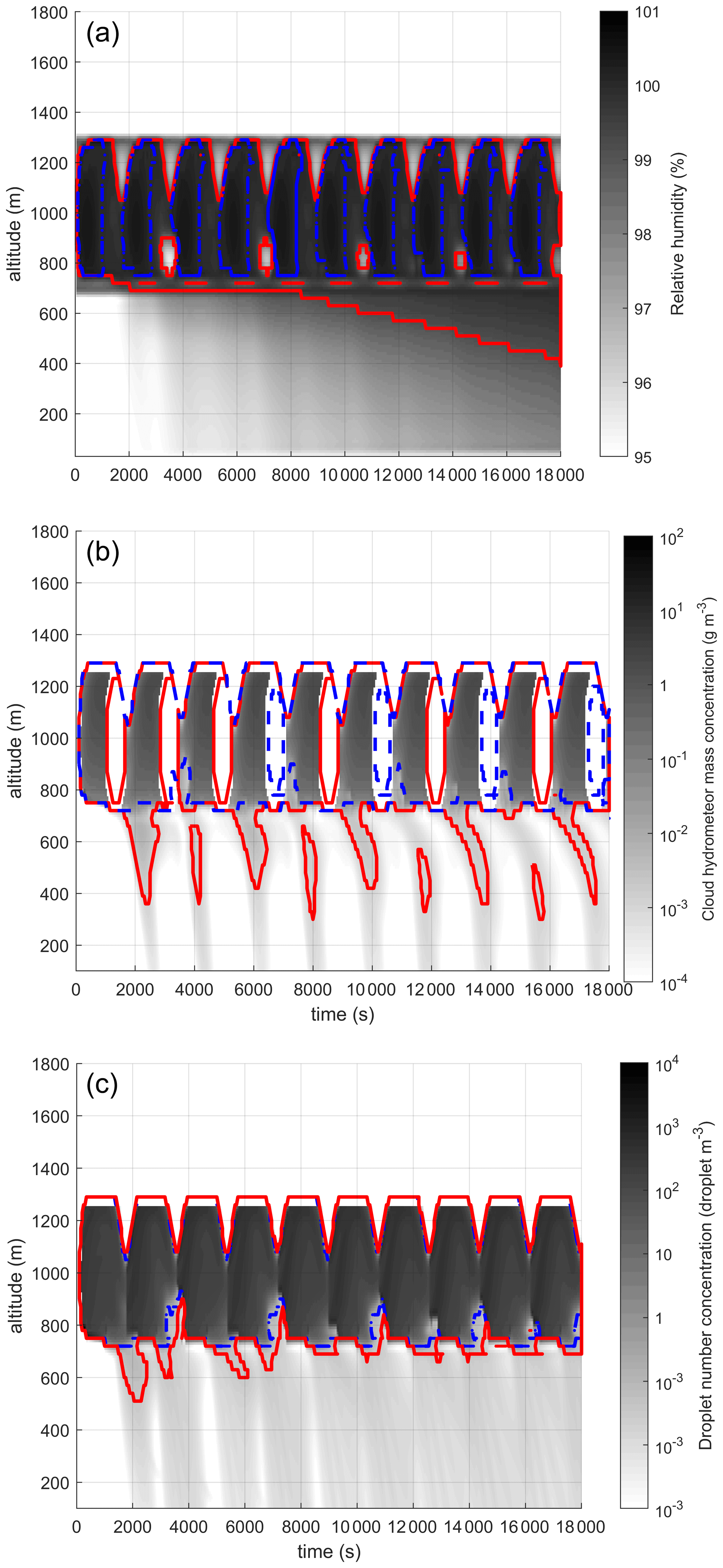
Figure 13 Test of different criteria to establish the contours of the simulated stratus. (a) Threshold based on relative humidity: () RH > 99 % and () RH > 100 %. (b) Threshold based on the mass concentration of hydrometeors with a diameter less than 64 µm: () mass concentration of cloud hydrometeors > 0.01 g m⁻³ and () mass concentration of cloud hydrometeors > 0.001 g m⁻³. (c) Threshold based on the concentration of hydrometeors: () ∫dℕ > 0.1 cm⁻³ and () $\int \mathrm{d}\mathbb{N}+\mathrm{d}\mathfrak{N}$ > 0.03 cm⁻³.

Based on these results, it is more difficult to delineate the contours of this stratus than those of the cumulonimbus. This is because, for these three criteria, only the droplet concentration shows a clear demarcation between precipitation and the cloud zone. Moreover, only this criterion gives stable cloud contours, regardless of the threshold value selected. This difference with respect to the cumulonimbus is mainly due to the size of the precipitating hydrometeors, which are much larger in the case of the cumulonimbus. Figure 14 shows that the particle size distribution mode for the number of raindrops, for the cumulonimbus, is close to a diameter of 1 mm, whereas it is 100 µm for the stratus. It is therefore easier with a cumulonimbus than with a stratus to define a size threshold distinguishing droplets (belonging to the cloud) from raindrops (belonging to precipitation). The criterion based on the mass concentration of hydrometeors exceeding 64 µm is therefore less effective under a stratus than under a cumulonimbus. To explain the poor performance of the criterion based on relative humidity, it is again the particle size that counts. As the droplets under the stratus are smaller than under the cumulonimbus, their velocities are lower and they reside for a longer time in the atmosphere – about 10 times longer. This longer residence time promotes the increase in relative humidity under the cloud and humidity saturation under the cloud. This makes it difficult to use this criterion to determine the boundary between rain and cloud for a stratus.

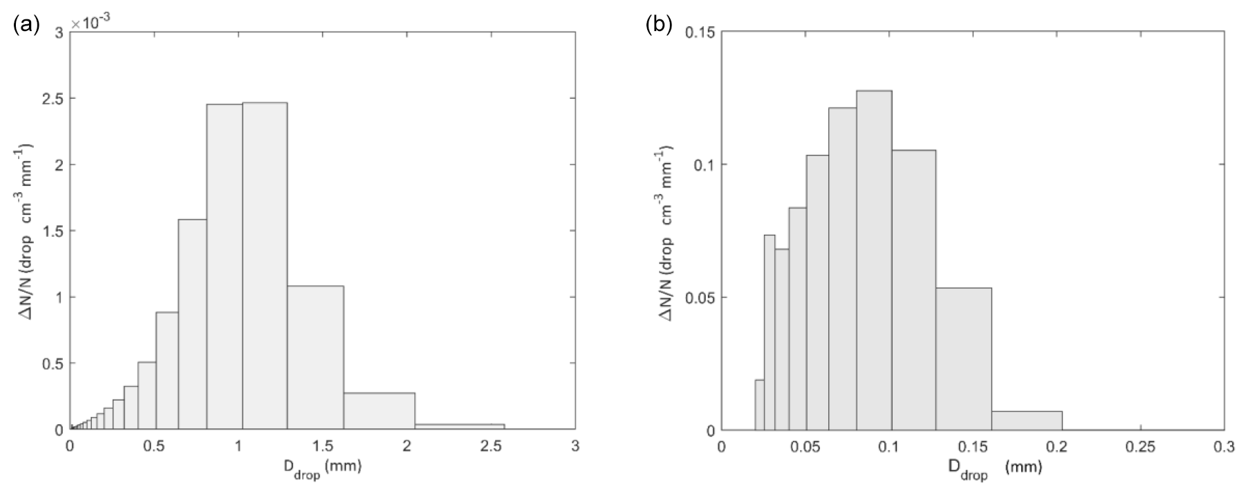
Figure 14 Particle size distributions of raindrops determined by DESCAM at ground level. (a) For cumulonimbus at time t = 3000 s. (b) For cumulonimbus at time t = 8200 s.

As previously, for the cumulonimbus, we search for a criterion to delimit cloud from rain. The same parameters as in Sect. 3.1 are investigated and are presented in Figs. 15–17.

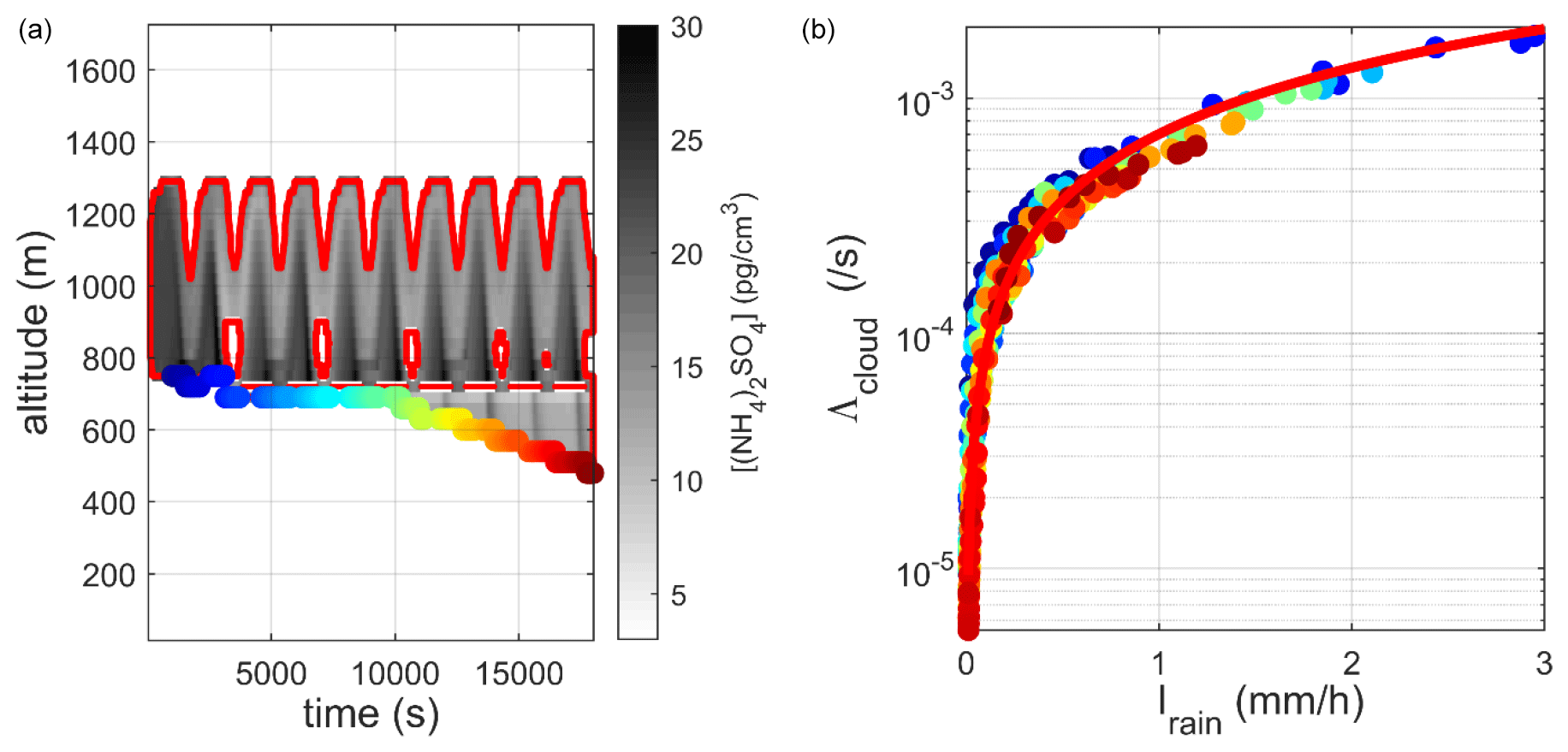
Figure 15 (a) Spatial–temporal distribution of the ammonium sulfate concentration in the cloud contour ( cloud contour for a relative humidity above 99 %). (b) Correlation between the scavenging coefficient and the precipitation intensity determined at the base of the cloud, adjusted by a power law ().

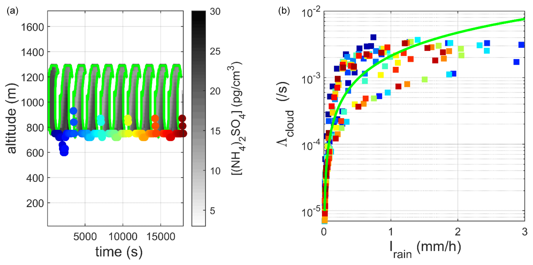
Figure 16 (a) Spatial–temporal distribution of the ammonium sulfate concentration in the cloud contour () (criterion based on the mass concentration of hydrometeors with a diameter greater than 64 µm with a threshold set at 0.01 g m⁻³). (b) Correlation between the scavenging coefficient and the precipitation intensity determined at the base of the cloud, adjusted by a power law ().

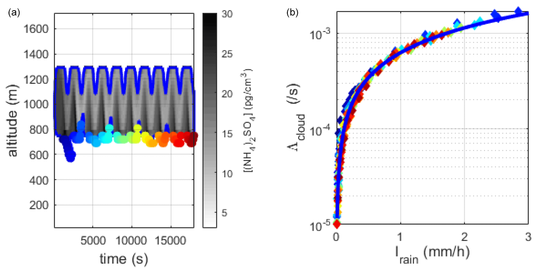
Figure 17 (a) Spatial–temporal distribution of the ammonium sulfate concentration in the contour of the cloud (criterion based on the concentration of hydrometeors with a threshold set at 0.01 particles cm⁻³). (b) Correlation between the scavenging coefficient and the precipitation intensity determined at the base of the cloud, adjusted by a power law ().

In these three figures, we observe that the contour introduced by Hiron (2017) for cumulonimbus (based on a separation between cloud water and precipitation water on the basis of a criterion on the size of hydrometeors; see Sect. 2.2) is no longer applicable for the stratus and gives highly dispersed scavenging coefficient results, particularly for low rain intensity (I < 2 mm h⁻¹). This is because, for this stratus, it is difficult to establish a strict boundary between a raindrop and a cloud droplet based on their sizes. However, the other two criteria yield bijective and similar relationships, in terms of both the cloud contours (Figs. 15a and 17a) and the adjusted power laws (Table 2). Unlike cumulonimbus, stratus contours appear to be reliable using a criterion based on relative humidity. This difference is related to the intensities of vertical flows in the cumulonimbus. Indeed, we observe in Fig. 5 that, in the simulated cumulonimbus, the downdraught flows can be very intense (up to 5 m s⁻¹), transporting air to the base of the cloud air masses with a lower mixing ratio and hence lower relative humidity.

Table 2 Adjustment of scavenging coefficients by power laws for the three types of contours studied.

These calculations show that, regardless of the type of simulated cloud, i.e. cumulonimbus or stratus, the criterion based on the hydrometeor concentration makes it possible to yield cloud contours that are stable (with little variation when the threshold value is varied) and for which the relationship between the scavenging coefficient and the rainfall intensity is the most biunivocal (Figs. 8–10 for cumulonimbus and Figs. 15–17 for stratus). This criterion is not directly accessible in meteorological models; however, examination of Figs. 10 and 17 suggests that the cloud base remains stable over time. It would therefore be possible to assess the altitude at which critical supersaturation is reached and to consider this altitude constant over a period that depends on the ratio between the size of the grid cell and the velocity of the horizontal flows.

3.3 Comparison with the literature and unification of the scavenging coefficient scheme for a cumulonimbus and a stratus

There are insufficient data to compare our theoretical findings with field study data. Few experimental data have established in situ scavenging coefficients for different types of clouds. Based on caesium-137 (¹³⁷Cs) deposition measured following the Fukushima Daiichi accident, Leadbetter et al. (2015) used the Met Office dispersion model NAME (Numerical Atmospheric-dispersion Modelling Environment) for the dispersion of the radioactive plume emitted during the accident, considering the meteorological data from the ECMWF model. The authors managed to determine the cloud scavenging coefficient which best suits the ground measurements of deposition (Kinoshita et al., 2011). In the same general approach, but using the IRSN ldX dispersion model (Groëll et al., 2014; Quélo et al., 2007) and meteorological data from the Meteorological Research Institute (MRI; Sekiyama et al., 2017), Quérel et al. (2021) established a very similar scavenging coefficient. These two schemes are compared in Fig. 18. The comparison is made using the κ value of ammonium sulfate. This decision is based on the findings of the Kaneyasu et al. (2012) study, which demonstrated the long-distance transport of ¹³⁷Cs by these particles – a distance particularly relevant for in-cloud scavenging.

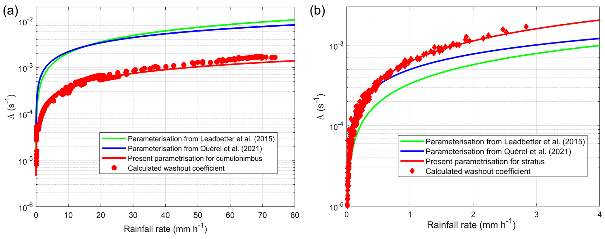
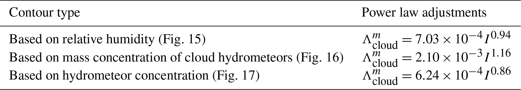
Figure 18 Comparison of the parameterisations established for a cumulonimbus (a) and a stratus (b), with the parameterisations established by Leadbetter et al. (2015) and Quérel et al. (2021) following the Fukushima accident.

In this figure, we observe that the application of our scheme to a stratus (Fig. 18b) concurs excellently with the parameterisation of scavenging by clouds established following the Fukushima accident, in particular with the parameterisation of Quérel et al. (2021). However, the application of our approach to cumulonimbus presents much greater differences. Indeed, over the entire rainfall intensity range, our results are on average 6 times lower than the correlations of Leadbetter et al. (2015) and Quérel et al. (2021). Two questions therefore arise:

• First, was there scavenging by cumulonimbus during the Fukushima accident? This would explain why it is difficult to compare our parameterisation of scavenging by cumulonimbus with those parameterisations deduced during the Fukushima accident.

• Next, why, for the same rainfall intensity, do our calculations show that cumulonimbus scavenges less than stratus?

We will address these two questions.

3.3.1 Was there scavenging by cumulonimbus during the Fukushima accident?

To answer this question, let us consider the distribution of rainfall intensities diagnosed from radar measurements by Saito et al. (2015a) during March 2011 in the Fukushima region (Fig. 19). These results show that 80 % of rain episodes diagnosed corresponded to rainfall intensities of less than 1.5 mm h⁻¹ and 97 % to intensities of less than 3.5 mm h⁻¹ (range of rainfall intensity produced at the base of the simulated stratus; Fig. 15) and that less than 0.01 % had intensities of more than 10 mm h⁻¹. In view of these results, it is not possible to completely exclude the presence of rain issuing from cumulonimbus over the period of the accident; however, if there was any, its contribution to the construction of the parameterisation of Leadbetter et al. (2015) and Quérel et al. (2021) is negligible.

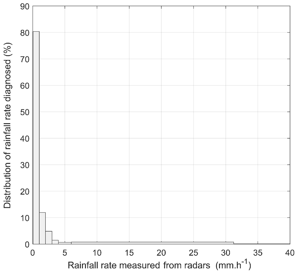
Figure 19 Distribution of rainfall intensity measured in the Fukushima region during March 2011 (Sekiyama et al., 2017).

3.3.2 How can the scavenging coefficient scheme for a cumulonimbus and a stratus be unified?

Our calculations show that cumulonimbus scavenges less than stratus under the same rainfall intensity. How can we understand this and unify the two equations? This phenomenon can be attributed to the significantly higher level of supersaturation observed in cumulonimbus clouds (Fig. 7a) compared to that in stratus cloud (Fig. 13a). Hence, if the supersaturation is higher, as is the case for cumulonimbus, for the same activated aerosol mass, these particles are diluted in a larger mass of water, as the condensation is also much greater (in reality, the activated aerosol mass increases significantly, since, as we have indicated previously, the activation diameter of the aerosols decreases as supersaturation increases). Let us therefore examine the impact of this effect of vapour condensation on the deduced parameterisation. In DESCAM, condensation is modelled by Eq. (17). This equation is taken from Pruppacher and Klett (1997, Chap. 13, Sect. 2). It results from the vapour diffusion equation applied to a droplet of diameter 𝒟_drop in the air with supersaturation 𝒮 and temperature T_∞, considering the thermodynamic equilibrium of the suspended drop within air using κ-Köhler theory.

$$\begin{array}{}\text{(18)}& \left\{\begin{array}{lcl}\frac{\mathrm{d}{\mathcal{D}}_{\mathrm{drop}}}{\mathrm{d}t}& =& \frac{\mathrm{4}}{{\mathcal{D}}_{\mathrm{drop}}}\frac{\mathcal{S}-y}{\frac{{\mathit{\rho }}_{\mathrm{w}}\mathcal{R}{T}_{\mathrm{\infty }}}{p_{\mathrm{sat},\mathrm{w}}{\mathfrak{D}}_v{M}_{\mathrm{w}}}+\frac{\mathcal{O}n{\mathit{\rho }}_{\mathrm{w}}}{k{T}_{\mathrm{\infty }}}\left(\frac{\mathcal{O}n{\mathit{\rho }}_{\mathrm{w}}}{\mathcal{R}{T}_{\mathrm{\infty }}}-\mathrm{1}\right)}\\ & & \\ y& =& \frac{\mathrm{4}{\mathit{\sigma }}_{\mathrm{w},{\mathcal{D}}_{\mathrm{drop}}}{M}_{\mathrm{w}}}{{\mathit{\rho }}_{\mathrm{w}}\mathcal{R}{T}_{\mathrm{\infty }}{\mathcal{D}}_{\mathrm{drop}}}-\mathit{\kappa }\frac{d_{\mathrm{ap}}^{{\mathrm{dry}}^{\mathrm{3}}}}{{{\mathcal{D}}_{\mathrm{drop}}}^{\mathrm{3}}}\end{array}\right.\end{array}$$

In this equation ℛ is the ideal gas constant, p_sat,w the saturating vapour pressure, $d_{\mathrm{ap}}^{\mathrm{dry}}$ the dry diameter of the aerosol, 𝒪n the latent heat of vaporisation of the water, ${\mathit{\sigma }}_{\mathrm{w},{\mathcal{D}}_{\mathrm{drop}}}$ the surface tension, k the thermal conductivity of the air, M_w and ρ_w the molar mass and density of the water vapour, and finally 𝔇_v the diffusion coefficient of the water vapour in air. As the Kelvin effect (linked to the curvature of the interface) and the solute effect become negligible very quickly after activation of the aerosol, this equation can be greatly simplified and reduced to ${\mathcal{D}}_{\mathrm{drop}}\mathrm{d}{\mathcal{D}}_{\mathrm{drop}}=\mathbb{C}\cdot \mathcal{S}\mathrm{d}t$, where ℂ is a constant, enabling it to be integrated analytically to give ${\mathcal{D}}_{\mathrm{drop}}\left(t\right)=\sqrt{{{\mathcal{D}}_{\mathrm{drop},t_{\mathrm{0}}}}^{\mathrm{2}}+\mathrm{2}\mathbb{C}\cdot \mathcal{S}\cdot t}$. Thus, to assess the effect of dilution of the aerosol in the droplet due to condensation, we can write

$$\begin{array}{}\text{(19)}& \begin{array}{rl}& {\displaystyle \frac{{\mathcal{D}}_{\mathrm{drop}}(t{)}_{\mathrm{stratus}}^{\mathrm{2}}}{{\mathcal{D}}_{\mathrm{drop}}(t{)}_{\mathrm{cumulonimbus}}^{\mathrm{2}}}}\\ & ={\displaystyle \frac{{{\mathcal{D}}_{\mathrm{drop},t_{\mathrm{0}}}}^{\mathrm{2}}+\mathrm{2}\mathbb{C}\cdot \langle \mathcal{S}{\rangle }_{\mathrm{stratus}}\cdot t_{\mathrm{stratus}}}{{{\mathcal{D}}_{\mathrm{drop},t_{\mathrm{0}}}}^{\mathrm{2}}+\mathrm{2}\mathbb{C}\cdot \langle \mathcal{S}{\rangle }_{\mathrm{cumulonimbus}}\cdot t_{\mathrm{cumulonimbus}}}}.\end{array}\end{array}$$

Note that in this equation, 𝒟_drop(t)_stratus and 𝒟_drop(t)_cumulonimbus are not the diameters of the droplets in the stratus and in the cumulonimbus but the diameters they would have had if only the condensation mechanism had caused them to grow. We are in fact seeking to assess how large the dilution of aerosol material in the droplets will be related to vapour condensation. There are other mechanisms modelled in DESCAM (such as coalescence or riming; Fig. 2) that lead to the growth of hydrometeors, without necessarily diluting the aerosols in the droplets. If there had only been the condensation mechanism, we could have used Fig. 14 directly to assess this dilution.

For long periods of time, further simplification can still be made because ${{\mathcal{D}}_{\mathrm{drop},t_{\mathrm{0}}}}^{\mathrm{2}}\ll {\mathcal{D}}_{\mathrm{drop}}(t{)}_{\mathrm{stratus}}^{\mathrm{2}}<{\mathcal{D}}_{\mathrm{drop}}(t{)}_{\mathrm{cumulonimbus}}^{\mathrm{2}}$. Finally, we can write

$$\begin{array}{}\text{(20)}& {\displaystyle \frac{{\mathcal{D}}_{\mathrm{drop}}(t{)}_{\mathrm{stratus}}^{\mathrm{2}}}{{\mathcal{D}}_{\mathrm{drop}}(t{)}_{\mathrm{cumulonimbus}}^{\mathrm{2}}}}={\displaystyle \frac{\cdot \langle \mathcal{S}{\rangle }_{\mathrm{stratus}}\cdot t_{\mathrm{stratus}}}{\langle \mathcal{S}{\rangle }_{\mathrm{cumulonimbus}}\cdot t_{\mathrm{cumulonimbus}}}}.\end{array}$$

In this equation, the times t_stratus and t_cumulonimbus are therefore the times necessary for the formation of precipitation under the cloud. For each of the cloud types, we observe in Figs. 6a and 12a that these times are very similar (≈ 2200 s), which allows us to write

$$\begin{array}{}\text{(21)}& {\displaystyle \frac{{\mathcal{D}}_{\mathrm{drop}}(t{)}_{\mathrm{stratus}}}{{\mathcal{D}}_{\mathrm{drop}}(t{)}_{\mathrm{cumulonimbus}}}}=\sqrt{{\displaystyle \frac{\langle \mathcal{S}{\rangle }_{\mathrm{stratus}}}{\langle \mathcal{S}{\rangle }_{\mathrm{cumulonimbus}}}}}.\end{array}$$

The numerical application of this equation highlights a condensation growth ratio with a factor of 2.3 between cumulonimbus and stratus. In mass, this coefficient corresponds to a dilution factor of 12. However, Fig. 18 shows that, with this new approach, we can calculate that cumulonimbus scavenges 6 times less than stratus. This explanation is therefore satisfactory in view of all the hypotheses that have been made, especially since we have considered that the activated aerosol mass remained constant when supersaturation increased. We therefore propose a new generic parameterisation to any type of cloud, which this time considers this condensation-related dilution effect (Eq. 22). This scavenging scheme is therefore corrected by a coefficient $\mathrm{1}/\langle \mathcal{S}{\rangle }_{\mathrm{cloud}}^{\mathrm{3}/\mathrm{2}}$, which characterises the dilution related to the growth of droplets by condensation:

$$\begin{array}{}\text{(22)}& {\mathrm{\Lambda }}_{\mathrm{cloud}}^m={\displaystyle \frac{\mathrm{5}\times {\mathrm{10}}^{-\mathrm{8}}}{\langle \mathcal{S}{\rangle }_{\mathrm{cloud}}^{\mathrm{3}/\mathrm{2}}}}{I}^{\mathrm{0.75}}.\end{array}$$

The application of this new correlation, presented in Fig. 20, shows an excellent match both for the cumulonimbus and for the simulated stratus. It remains to be considered whether supersaturation is accessible in numerical weather prediction (NWP) models and, if so, if the horizontal resolutions of 1 to 10 km of such models are sufficiently representative of a real cloud.

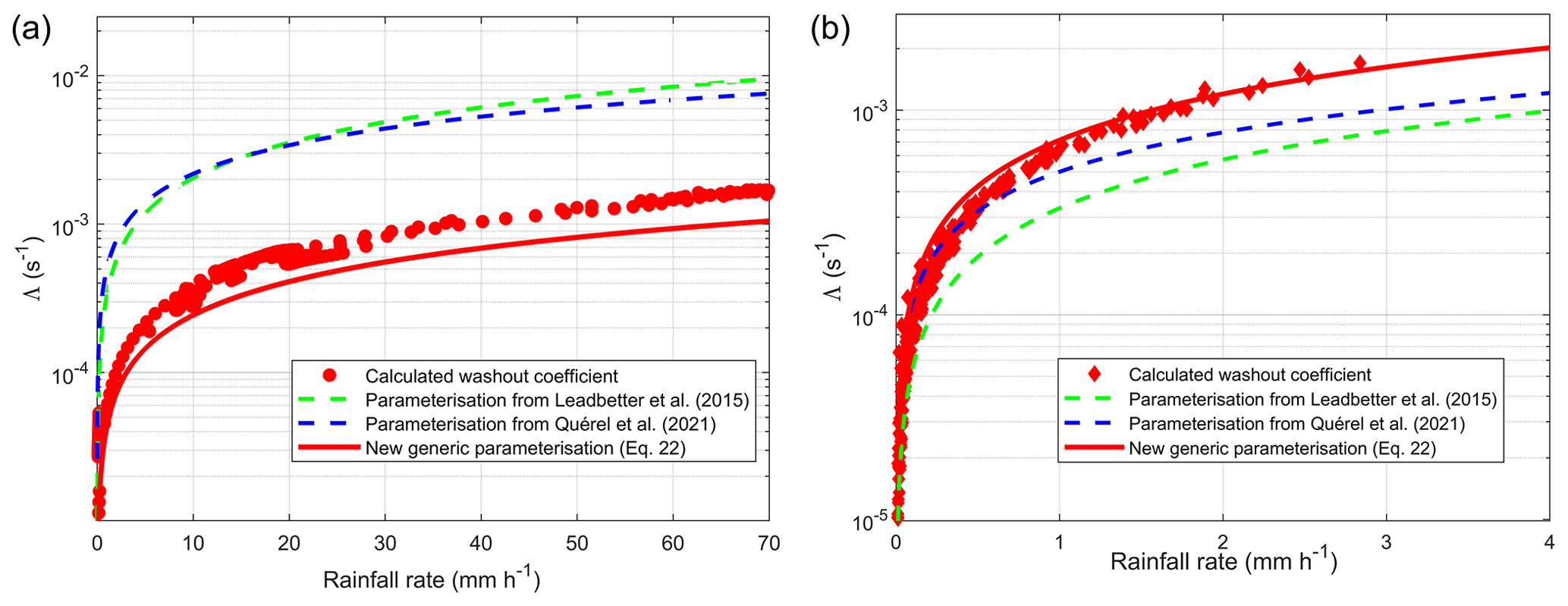
Figure 20 Comparison of the newly developed correlation (Eq. 21) with the scavenging modelled by DESCAM for a cumulonimbus and a stratus.

4 Conclusions

The in-cloud scavenging scheme established in this article shows a dependence on rain intensity and average supersaturation in the cloud. Supersaturation allows the scheme to be applicable to both cumulonimbus and stratus clouds. If supersaturation in the cloud is not accessible, it is still possible to apply a different scheme for convective clouds and stratiform clouds. However, since this boundary between the two cloud types may be ambiguous, it is preferable to apply the scheme with supersaturation if available.

This scavenging scheme is based on the microphysical cloud model DESCAM. This model allows for a fine-scale description of the life cycle of a cloud up to precipitation development. It tracks particle, crystal, and droplet particle size distributions and models all the water phase changes and, above all, how aerosol particles impact them. The in-cloud scavenging scheme is established by calculating the mass fluxes of particle material exiting the cloud that are included in precipitation hydrometeors (both liquid and solid) and is based on the mass of particles initially present in the cloud volume.

This calculation of cloud volume has proved to be a complex issue, in particular for establishing the altitude of the cloud base, especially when rain occurs. The most relevant method to identify the cloud base in this study has been proved to be the one using the number of hydrometeors, rather than the relative humidity or the mass of the hydrometeors. The problem with this method is that this information on the number is not available for most NWP models. The use of the in-cloud scavenging scheme must be based on a diagnostic independent of the altitude of the base – and the summit – of the cloud.

In the case of stratus cloud, the parameterisation obtained with DESCAM is close to those parameterisations currently used in the NAME and ldX atmospheric dispersion models, which were established on the basis of the Fukushima accident. As the precipitation that caused deposition of radioactive particles following the accident was largely generated by stratiform clouds, this study confirms a posteriori the choice of the in-cloud deposition scheme used to study radioactive deposition following the Fukushima accident and can be extended to all types of clouds.

In future works, this deposition scheme will be used with confidence to study deposition. As an example, it can be used for the deposition of radon progeny (Quérel et al., 2022) to statistically measure the impact of this scheme in relation to the existing corpus.

Beyond the applications and validation of the scheme described in this article, the scheme itself is currently being refined. First of all, we are working on establishing an in-cloud scavenging rate that will depend on particle size. This important issue is discussed in Sect. 2.3 and requires some modifications to the model to establish a model spectrally. This will make it possible to apply a finer-scale scheme to the atmospheric models with a spectral representation of the particles.

The influence of the coefficient κ of κ-Köhler theory can be also examined. This will make it possible to measure the importance of the physical–chemical properties of the particles, assessing what error is made by applying the same scavenging rate for a hygroscopic aerosol (salt or sulfate) and a non-hygroscopic aerosol (soot, desert dust).

The initial particle size distribution of aerosols could also have a significant influence on the final scavenging rate. A distribution centred on 100 nm will not create the same cloud as the same total mass centred around 5 µm particles. This aspect must be assessed.

The question of evaporation of droplets between the cloud base and the ground has not yet been addressed. The scheme developed is based on the precipitation intensity at the cloud base, but in the models the precipitation intensity is diagnosed on the ground. This is important for the applicability of the scheme, and this difference can lead to errors, especially in the event of high droplet evaporation.

Finally, it has not yet been established whether this scheme is as effective when applied to a model whose spatial resolution is lower than that of DESCAM, as is the case for all global climate models (GCMs) and atmospheric transport models (ATMs).

The work still to be carried out will make it possible to best define the scope of validity of this new scheme for in-cloud aerosol scavenging, as well as the uncertainties associated with this model. This will enable the scheme to be used in full knowledge of the facts and according to the highest scientific standards.