the Creative Commons Attribution 4.0 License.
the Creative Commons Attribution 4.0 License.
 | 30 Aug 2024
Elevated oxidized mercury in the free troposphere: analytical advances and application at a remote continental mountaintop site
Eleanor J. Derry
Tyler R. Elgiar
Taylor Y. Wilmot
Nicholas W. Hoch
Noah S. Hirshorn
Peter Weiss-Penzias
Christopher F. Lee
John C. Lin
A. Gannet Hallar
Rainer Volkamer
Seth N. Lyman
Mercury (Hg) is a global atmospheric pollutant. In its oxidized form (HgII), it can readily deposit to ecosystems, where it may bioaccumulate and cause severe health effects. High HgII concentrations are reported in the free troposphere, but spatiotemporal data coverage is limited. Underestimation of HgII by commercially available measurement systems hinders quantification of Hg cycling and fate. During spring–summer 2021 and 2022, we measured elemental (Hg0) and oxidized Hg using a calibrated dual-channel system alongside trace gases, aerosol properties, and meteorology at the high-elevation Storm Peak Laboratory (SPL) above Steamboat Springs, Colorado. Oxidized Hg concentrations displayed diel and episodic behavior similar to previous work at SPL but were approximately 3 times higher in magnitude due to improved measurement accuracy. We identified 18 multi-day events of elevated HgII (mean enhancement of 36 pg m−3) that occurred in dry air (mean ± SD of relative humidity = 32 ± 16 %). Lagrangian particle dispersion model (HYSPLIT–STILT, Hybrid Single-Particle Lagrangian Integrated Trajectory–Stochastic Time-Inverted Lagrangian Transport) 10 d back trajectories showed that the majority of transport prior to events occurred in the low to middle free troposphere. Oxidized Hg was anticorrelated with Hg0 during events, with an average (± SD) slope of −0.39 ± 0.14. We posit that event HgII resulted from upwind oxidation followed by deposition or cloud uptake during transport. Meanwhile, sulfur dioxide measurements verified that three upwind coal-fired power plants did not influence ambient Hg at SPL. Principal component analysis showed HgII consistently inversely related to Hg0 and generally not associated with combustion tracers, confirming oxidation in the clean, dry free troposphere as its primary origin.
- Article
(9098 KB) - Full-text XML
- BibTeX
- EndNote


Mercury (Hg) is a global pollutant that can be emitted to the atmosphere from both natural and anthropogenic sources. Humans have changed the Hg biogeochemical cycle through industrial development and land use practices that have increased atmospheric Hg concentrations and altered reservoir distributions (Obrist et al., 2018; Driscoll et al., 2013; Selin, 2009). Mercury is a toxin that can cause neurological and cardiovascular health effects depending on the duration, magnitude, and chemical form of exposure (Lyman et al., 2020a; Driscoll et al., 2013; Selin, 2009). In the atmosphere, Hg exists as gaseous elemental Hg (Hg0; GEM), gaseous HgII – commonly referred to as GOM (gaseous oxidized mercury) or RGM (reactive gaseous mercury) – and particulate-bound mercury (PBM). Elemental Hg is relatively inert and has an atmospheric lifetime on the scale of months (Bishop et al., 2020). Oxidized Hg (HgII = GOM + PBM), however, is much more reactive and water soluble, resulting in an atmospheric lifetime on the scale of days to a week in the planetary boundary layer (PBL) (Lyman et al., 2020a). Thus, when Hg0 undergoes oxidation to form HgII, it is much more readily deposited into ecosystems, where it can methylate and bioaccumulate within food systems, with potential environmental and health consequences (Driscoll et al., 2013; Selin, 2009).
While international and domestic regulations have led to decreases in global background ambient Hg concentrations (Obrist et al., 2018; Lyman et al., 2020a), local conditions can vary significantly because of differences in the magnitude of urban and industrial emissions (Driscoll et al., 2013). Global background terrestrial Hg0 concentrations also vary spatially; concentrations in the Northern Hemisphere reportedly range from 1.5 to 1.7 ng m−3, and those in the Southern Hemisphere range from 1.0 to 1.3 ng m−3 (Sprovieri et al., 2016), caused by the higher concentration of urban areas and greater anthropogenic emissions in the Global North (Mao et al., 2016). Mercury species have also been shown to exhibit variability with altitude. Elemental Hg is typically well mixed in the PBL, while HgII has been shown to increase in concentration with elevation (Swartzendruber et al., 2006; Faïn et al., 2009; Lyman and Jaffe, 2012; Gratz et al., 2015; Shah et al., 2016). The atmosphere is considered to be a minor reservoir of Hg (∼ 5 Gt) compared to soil (1450 Gt) and marine ecosystems (280 Gt), but it is the dominant pathway for Hg inputs to ecosystems via deposition (Driscoll et al., 2013; Obrist et al., 2018; Lyman et al., 2020a). Oxidized Hg can be deposited via precipitation or dry deposition to both terrestrial and marine ecosystems. Recent work has posited that global models underestimate the importance of Hg0 uptake by vegetation and oceans and are therefore biased toward HgII deposition (Sonke et al., 2023; Fu et al., 2021).
The chemical oxidation-reduction mechanisms of Hg in the atmosphere, which determine its environmental fate, are complex and not fully understood (Dibble et al., 2020; Lyman et al., 2020a; Shah et al., 2021; Castro et al., 2022). Previous studies have indicated multiple possible major oxidants of Hg in the atmosphere. While Hg oxidation can occur in the stratosphere, driven by a photosensitized oxidation mechanism (Saiz-Lopez et al., 2022), as well as in both the marine and continental boundary layers (Lyman et al., 2020a), recent studies have suggested that Hg oxidation occurs primarily in the free troposphere and the leading oxidants are halogens, such as atomic bromine (Br), and the hydroxyl radical (OH) (Dibble et al., 2020). Oxidation in the free troposphere is thought to be driven by a two-step mechanism, in which ozone (O3) acts as a secondary oxidant (Shah et al., 2021; Castro et al., 2022). Previous studies have reported Br-initiated oxidation in the free troposphere (Gratz et al., 2015; Coburn et al., 2016). A companion paper to this study further demonstrated that iodine-initiated oxidation may compete with Br- and OH-initiated oxidation at cold temperatures and may be important for understanding the Hg oxidation mechanism (Lee et al., 2024). This chemical cycling creates a pool of HgII within the free troposphere (Lyman and Jaffe, 2012; Shah et al., 2016; Weiss-Penzias et al., 2015).
Large uncertainties exist in the rate constants of the Hg oxidation mechanism, and there remains a shortage of experimental data (Castro et al., 2022). Part of this uncertainty comes from limitations in commercial instrument and measurement accuracy (Jaffe et al., 2014; Lyman et al., 2020b; Gustin et al., 2024). Most measurements of atmospheric HgII to date have relied on KCl denuders, which exhibit a low bias (Lyman et al., 2020b, and references therein). The extent of this low bias cannot be directly quantified, as most HgII measurements have been uncalibrated (Gustin et al., 2015; Jaffe et al., 2014). Thus, these datasets likely suffer from an underestimation of atmospheric HgII concentrations (Lyman et al., 2020b).
Previous studies at mountaintop observatories in the US, Taiwan, and France have examined temporal trends in atmospheric Hg concentrations and consistently showed evidence of high concentrations of HgII in the clean, dry air of the free troposphere (Swartzendruber et al., 2006; Faïn et al., 2009; Sheu et al., 2010; Timonen et al., 2013; Fu et al., 2016). One such site is Storm Peak Laboratory (SPL), a high-elevation, continental research station in the US Rocky Mountains. Past work at SPL documented transitions between the PBL and the free troposphere using long-term measurements of aerosols and trace gases (Collaud Coen et al., 2018). Moreover, studies by Obrist et al. (2008) and Faïn et al. (2009) investigated the influence of anthropogenic Hg sources, as well as the effects of meteorology and air mass chemical composition on speciated Hg compounds. However, these and other mountaintop studies historically relied on instrumentation that likely underestimated HgII concentrations (Lyman et al., 2020b).
In this study, we employed a calibrated Hg measurement technique with higher time resolution and improved measurement accuracy compared to other available methods (Lyman et al., 2020b; Elgiar et al., 2024). Data were collected at SPL above Steamboat Springs, Colorado, during two 6-month periods in spring and summer 2021 and 2022. We examined meteorology, air mass composition, and atmospheric transport during periods of elevated HgII to more accurately quantify the concentrations of HgII and to identify its origins in a continental atmosphere.
2.1 Site description
The data used in this study were collected at Storm Peak Laboratory (3220 ; 40.455° N, 106.744° W) above Steamboat Springs, Colorado. SPL is a permanent high-elevation research facility within the Rocky Mountains along the Continental Divide. The site is optimally located to characterize the remote continental atmosphere and transitions between the PBL and the free troposphere (Faïn et al., 2009; Collaud Coen et al., 2018). SPL receives prevailing westerly winds, creating a clear upwind fetch (Faïn et al., 2009). The site is located east of the agricultural Yampa Valley and approximately 19 km from downtown Steamboat Springs (Fig. A1). SPL is also located east and downwind of three coal-fired power plants, located in Hayden, Colorado; Craig, Colorado; and Vernal, Utah, but otherwise sits in a relatively remote location with few nearby point sources that could influence atmospheric composition at the laboratory.
2.2 Data collection
2.2.1 Dual-channel measurements of Hg0 and HgII
The Utah State University (USU) dual-channel Hg measurement system operated at SPL from 12 March 2021 to 11 October 2021 and 3 March 2022 to 22 September 2022. The operation, validation, quality assurance, and quality control of this system at SPL are described in detail in Elgiar et al. (2024). Briefly, the dual-channel system pulls ambient air through the main Teflon-coated aluminum inlet at a rate of 9 slpm into a weatherproof box containing a thermal converter and a pair of in-series cation exchange membranes. The thermal converter is constructed of quartz, packed with quartz chips, and maintained at a temperature of 650 °C to convert HgII to Hg0 such that total Hg is measured (THg = HgII + Hg0) (Lyman et al., 2020b). The cation exchange membranes remove HgII from the sample airstream, allowing only Hg0 to pass through (Miller et al., 2019). A valve switches between the thermal converter and the cation exchange membranes every 5 min. During each 5 min period, two 2.5 min measurements are recorded by the downstream Tekran 2537X Hg0 vapor analyzer. Oxidized Hg concentrations are computed as the difference between (a) two consecutive 2.5 min THg measurements averaged together and (b) the average of the 2.5 min Hg0 measurement preceding and the one following the consecutive THg measurements. As such, the system generates a complete set of Hg measurements (THg, Hg0, HgII) every 10 min. Inlet and sample lines are maintained at a temperature of 110 °C to minimize contamination and wall losses.
Elemental mercury vapor injections on the Tekran 2537X were performed every 6 to 8 weeks using a Tekran 2505 calibration unit to verify the permeation rate of the internal calibration source. The soda lime trap upstream of the 2537X (used to prevent passivation of the internal gold traps) and the dual-channel system's cation exchange membranes were replaced every 2 weeks, while the inlet was replaced every 4 weeks. The dual-channel system was also verified for measurement accuracy with an International System of Units-traceable (SI) calibrator that injected known amounts of Hg0, HgBr2, and HgCl2 into the inlet on a weekly basis, as described in Elgiar et al. (2024). All final Hg0 and HgII concentrations were increased by 8 % to account for a suspected bias in the Dumarey equation used for calculating vapor pressure of Hg0 for manual injections (Elgiar et al., 2024; de Krom et al., 2021). The 1 h average detection limits for HgII measurements were 12 ± 7 pg m−3 (mean ± 95 % confidence interval of weekly detection limit tests conducted throughout the measurement season) in 2021 and 6 ± 2 pg m−3 in 2022. The detection limits were calculated as 3 times the standard deviation of measurements of HgII during times when both channels were sampling HgII-free air. The percent standard uncertainty for Hg0 and HgII with the dual-channel system, which takes into account the uncertainty budget for the Tekran 2537X analyzer (following the methodology of Brown et al., 2008), as well as the performance of the dual-channel component of the system, was 8 % (Elgiar et al., 2024). The placement of the dual-channel component of the system (e.g., the box containing the thermal converter and cation exchange membranes) outdoors and immediately upstream of the inlet and the development of an automated calibration system for Hg0 and HgII compounds were both key improvements to the dual-channel system for the present study.
Table 1Summary statistics of Hg0, HgII, trace gas, and aerosol PM1 (particulate matter < 1 µm) scattering (σsp) measurements by season and for each study year at SPL. The intermittent negative concentrations for HgII observed between 2–11 May 2021 (2 % of hourly data) and one value in 2022 were excluded from the values reported in this table. See Sect. 2.2.1 for details.
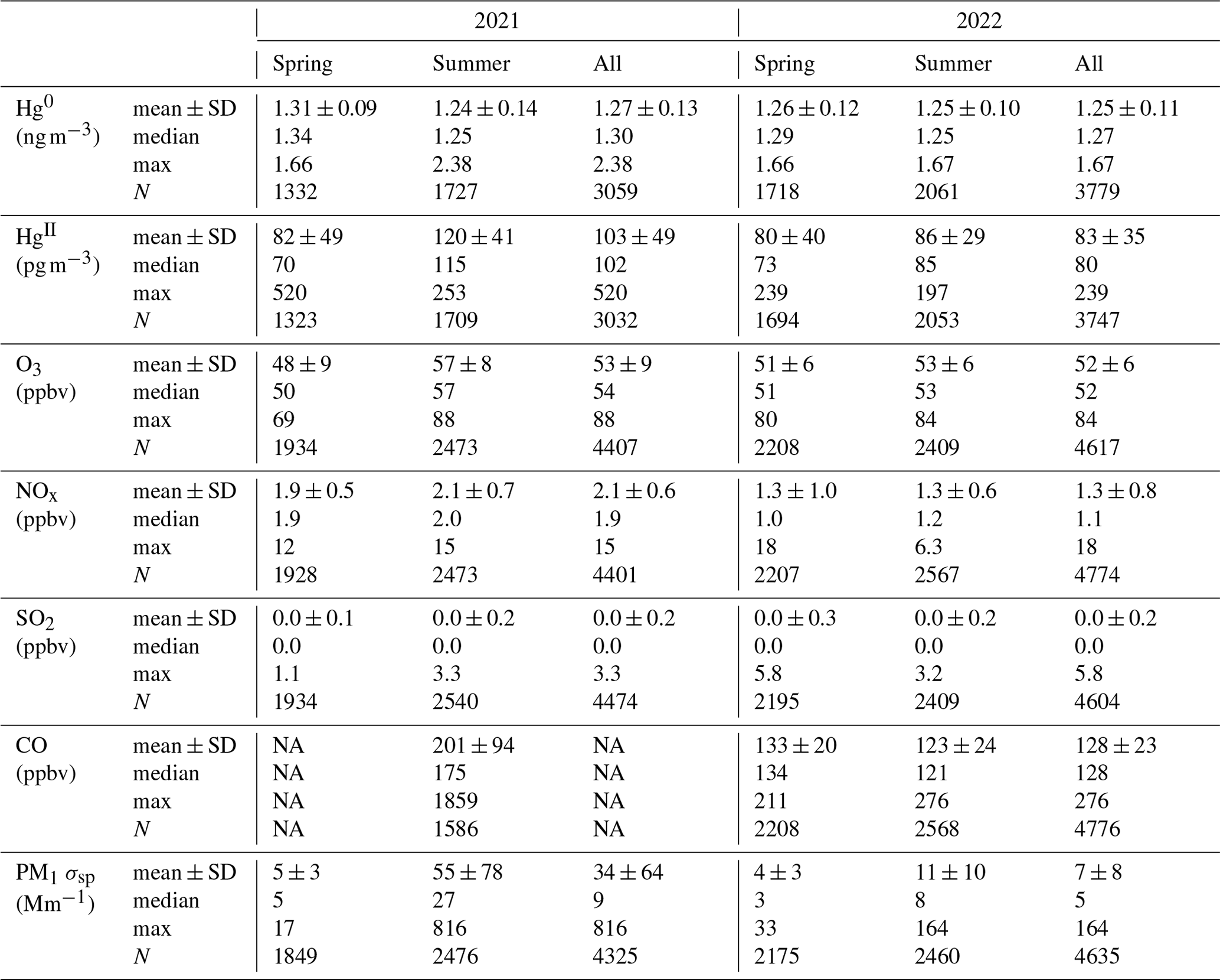
NA: all instances of “NA” in tables refer to “not available”.
The dual-channel system may occasionally report negative values for HgII when the Hg0 concentration is greater than the corresponding THg measurement used in the difference calculation (Dunham-Cheatham et al., 2023). This may occur in plumes of rapidly changing concentrations or for other reasons related to instrument performance that are as yet not fully understood. In this study, negative concentrations of hourly averaged HgII were computed only intermittently between 2–11 May 2021, most notably during two approximately 24 h periods between 2 and 4 May, as well as for approximately 10 h on 10 May. We therefore excluded several pairs of hourly averaged HgII and Hg0 concentrations during this early May 2021 period (n = 65; 2 % of the 12 March–15 September 2021 data). Removing these points did not change the 2021 mean, median, or standard deviation of Hg0 within the measurement precision shown in Table 1; the spring 2021 mean ± SD decreased from 1.32 ± 0.10 to 1.31 ± 0.09 ng m−3. For HgII, the exclusion of these values increased the 2021 mean ± SD from 101 ± 52 (median of 101) pg m−3 to 103 ± 49 (median of 102) pg m−3 and increased the spring 2021 mean ± SD from 77 ± 54 (median of 67) pg m−3 to 82 ± 49 (median of 70) pg m−3. In 2022, there was only one negative value for the hourly averaged HgII concentrations, and that value, along with the corresponding Hg0 concentration, was also removed. Other extended gaps in the datasets, related to instrument malfunction or operator error, included the periods from 12 May to 6 June, 29 June to 9 July, and 2 to 10 August in 2021, as well as 27 June to 1 July and 16 to 23 August in 2022.
2.2.2 Criteria gas and meteorological measurements
Several criteria gases and meteorological parameters related to this study were continuously measured at SPL. Meteorological data were measured on the roof of SPL at a height of 10 m above ground level () at a 5 min time resolution. Measured meteorological parameters included temperature, relative humidity (RH), wind speed and direction, and barometric pressure. These data were quality-assured and made publicly available by MesoWest (https://mesowest.utah.edu, last access: 5 June 2023). We computed water vapor mixing ratios using a combination of measured temperature, RH, and barometric pressure and the theoretical expression of the Clausius–Clapeyron equation.
Ozone, nitrogen oxides (NOx), sulfur dioxide (SO2), and aerosol properties such as scattering and absorption at 450, 550, and 700 nm were measured at a time resolution of 1 min and calibrated daily. Ozone was measured using a Thermo model 49i analyzer with a precision of 1.0 ppbv. Nitrogen oxides were measured with a Thermo model 42i NO–NO2–NOx analyzer with a precision of 0.2 ppbv. Sulfur dioxide was measured using a Thermo model 43i analyzer with a precision of the greater value of either 1 % or 1 ppbv. Aerosol properties were measured with a TSI model 3562 nephelometer. Analysis for this paper relied on PM1 scattering (PM1 σsp) as the representative aerosol metric, in part for direct comparison with related studies (e.g., Timonen et al., 2013) and because the aerosol absorption data had more frequent gaps. Aerosol data were corrected to STP (standard temperature and pressure) conditions and quality-controlled and quality-assured by NOAA ESRL GML (National Oceanic and Atmospheric Administration Earth System Research Laboratories Global Monitoring Laboratory) (Andrews et al., 2019). Carbon monoxide (CO) was measured beginning on 9 July 2021 with a Teledyne model 300E, from which average values were logged every 2.5 min in 2021 and every minute in 2022. The analyzer performed an automatic zero every 4 h in CO-free air; routine on-site spans for CO could not be performed due to COVID-19-related site access limitations, but based on those able to be performed before, during, and after the study, the measurement accuracy was estimated to be within ± 25 %.
2.3 Data analysis and modeling techniques
2.3.1 Statistical treatment of data
The measurement data were averaged to 1 h intervals corresponding to the beginning of each hour to compare all the variables at the same time step. Analyses in the present paper focus specifically on measurements made from 13 March 2021 to 15 September 2021 and from 3 March 2022 to 15 September 2022, encompassing two complete 6-month periods each year. We defined spring as 1 March to 31 May and summer as 1 June to 15 September given prior knowledge of the seasonal climatology and transport patterns (Obrist et al., 2008; Hallar et al., 2016). For example, past work has shown that trans-Pacific transport as well as stratospheric subsidence occur more commonly in springtime (Hallar et al., 2016), while summertime air masses at SPL are frequently impacted by biomass burning and different transport patterns (Obrist et al., 2018). Additionally, Hg concentrations have been shown to vary seasonally within the Northern Hemisphere, driven largely by seasonal meteorology (Xu et al., 2022; Custódio et al., 2022).
In this study, statistical significance was defined as p < 0.05. Reduced major axis (RMA) regressions were used to calculate linear regression slopes to account for uncertainty in both variables, as recommended for air quality data (Ayers, 2001). Correlation analysis was performed using Pearson's correlation coefficients (R), and comparisons of means were calculated using two-tailed independent sample t tests and Mann–Whitney U tests.
Lastly, we estimated that at least one-third of the 10 min averaged measurements in June–September 2021 showed evidence of smoke presence, whereas this was detected in less than 5 % of data for the same time frame in 2022. The presence of smoke was based on preliminary criteria of CO ≥ 150 ppbv, PM1 σsp ≥ 30 Mm−1, and PM10 σsp ≥ 35 Mm−1 for a minimum of 1 h and confirmation of overhead smoke using the National Oceanic and Atmospheric Administration Hazard Mapping System Fire and Smoke Product (NOAA HMS) (accessed via the AirNow Tech Navigator, 2023).
Table 2Event mean ± SD for HgII, Hg0, RH, O3, CO, and PM1 σsp.
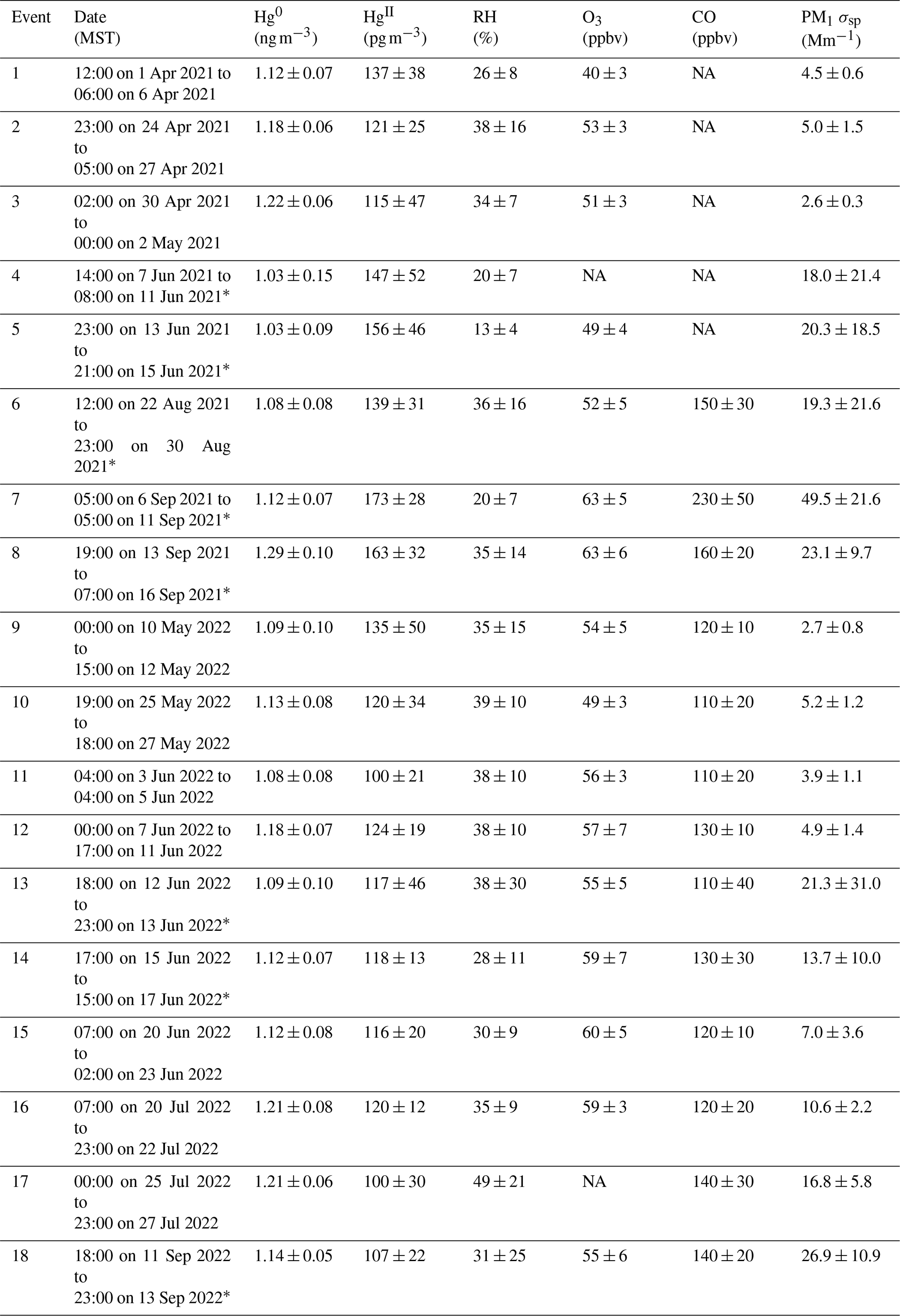
∗ These events had evidence of smoke from local or regional biomass burning.
2.3.2 Identification of events of elevated oxidized mercury
Events of elevated HgII were initially defined as time periods when HgII concentrations exceeded the seasonal mean by at least 1 standard deviation (Table 1) for a minimum of 24 h. Adjacent periods of elevated HgII were counted as the same event if they appeared to represent the same air mass, based on concurrent meteorological and trace gas measurements (e.g., consistently similar Hg0, HgII, and trace gas concentrations and RH before and after a brief intrusion of air associated with the boundary layer). Additional hours were then included in the events at the beginning and end of periods of high HgII in order to capture the transition between air mass conditions. In total, we identified 18 events of prolonged high HgII in the 2021 and 2022 measurement periods (Table 2). All events had at least 85 % Hg data coverage. We characterized the events through statistical analysis of Hg, trace gases, and meteorology as well as air mass transport analysis (Sects. 3.2.1 and 3.2.2) in order to understand the origins of the air masses containing elevated concentrations of HgII. We also analyzed the June 2022 measurement period as a case study because it contained relatively continuous records of all measured species and included five distinct events of high HgII (Events 11–15; Table 2), separated by periods of depleted HgII that were defined as Non-events 1–5 (Sect. 3.2.3). Non-event 5 was made to include the 24 h following the end of Event 15. Analysis of the measurement data within and between events was complemented by a simulation of air mass origins, as described below.
2.3.3 Air mass transport analysis using HYSPLIT–STILT
The Hybrid Single-Particle Lagrangian Integrated Trajectory model, integrating features from the Stochastic Time-Inverted Lagrangian Transport model (HYSPLIT–STILT), is a Lagrangian particle dispersion model (Loughner et al., 2021; Lin et al., 2003) that was used to investigate the history of air masses arriving at SPL. For each of the 18 events and 5 non-events presented here, an ensemble of 1000 air parcels were released at SPL at 3 h intervals and traced for 240 h backward in time. The air parcels were initialized at 5 m above ground level and transported with stochastic motions (simulating turbulence) with HYSPLIT–STILT, driven by meteorological fields from the 3 km meteorology from the High-Resolution Rapid Refresh model (HRRR; Dowell et al., 2022; NOAA Air Resources Laboratory, 2024), as well as the 0.25° × 0.25° meteorology from the Global Forecast System (GFS; NOAA Air Resources Laboratory, 2024). Nesting HRRR meteorology within the relatively coarse GFS meteorological fields was necessary for simulating atmospheric transport over the Pacific Ocean. Along each air parcel's backward trajectory, position, the mixed-layer depth, precipitation rate, RH, temperature, and total cloud cover from the meteorological fields were sampled at 1 min intervals, providing insight into the spatial origin and meteorological conditions associated with each air mass.
2.3.4 Principal component analysis
We used the principal component analysis (PCA) multivariate factor technique to investigate the interrelationships between measured variables and identify broad patterns in air mass composition at SPL. Factor analysis methods have been utilized in several studies involving continuous atmospheric measurements in both urban/industrial and remote environments (Swartzendruber et al., 2006; Liu et al., 2007; Lynam and Keeler, 2006; Tokarek et al., 2018). Other methods such as positive matrix factorization (PMF) or non-negative matrix factorization (NMF) are recommended for quantitative identification of source–receptor relationships (Hopke and Jaffe, 2020) and are often applied in urban/industrial environments using data from a common instrument (e.g., a suite of volatile organic compound (VOC) measurements, as in Peng et al., 2022, and Gkatzelis et al., 2021). Though PCA is an unweighted least-squares method (Hopke and Jaffe, 2020), it has the advantage in the present study as an exploratory approach that can indicate both the magnitude and sign of the statistical relationships between variables (Jolliffe and Cadima, 2016). PCA is also advantageous at SPL where the combined dataset came from multiple continuous instruments with different measurement scales, and the objective was to use the underlying nature of statistical covariances to broadly characterize air mass compositions at SPL. PCA results were considered in tandem with the case study analysis to extrapolate the conditions under which enhancements in HgII or other variables were observed.
We applied PCA with varimax rotation and Kaiser normalization (IBM SPSS v29.0.1.1) to each of the four sampled seasons in this study. Spring and summer were modeled separately, considering prior knowledge of seasonal climatology and transport (Obrist et al., 2008; Hallar et al., 2016), because air mass composition at SPL in summer 2021 was intermittently impacted by local or regional wildfire smoke (Sect. 2.3.1) and because the CO instrument was not operational in spring 2021. We additionally modeled the full 2022 measurement period (1 March–15 September 2022) because there was notably less evidence for regional wildfire smoke in the air at SPL during summer 2022.
Input variables for PCA included Hg0, HgII, CO, O3, NOx, PM1 σsp, water vapor mixing ratio, and barometric pressure. Wind speed was excluded given its weak communalities in the output for most seasons. Although HgII was generally better correlated with RH (Sect. 3.2.1), the water vapor mixing ratio was used in place of RH in PCA as a potentially better indicator of atmospheric moisture content and because the upper bound of 100 % in RH measurements influences its statistical distribution. Moreover, after filtering the data for RH < 85 % to exclude periods when SPL may have been in cloud, the Pearson's R and p values for HgII vs. water vapor mixing ratio in each season did not substantially change in comparison to HgII vs. RH, indicating that water vapor mixing ratio was a robust predictor of HgII, even if not as strong as RH (Table A1). Sulfur dioxide was excluded because it was near 0 ppbv on average (Table 1), with enhancements observed only in short-lived fresh combustion plumes.
Prior to running PCA, variables with |skewness| larger than 0.5 (moderate skew) or larger than 1.0 (high skew) were log-transformed. If the |skewness| did not improve, then the non-log-transformed variable was retained. All variables with |skewness| > 1.0 improved following log transform. In most seasons, PM1 σsp also needed to be shifted by its minimum before transformation due to small negative values. Data points 3 standard deviations above or below the dataset mean were then removed as outliers (< 2 % of values for each variable). Lastly, variables were standardized (mean of 0, standard deviation of 1) by subtracting that variable's mean and dividing by the standard deviation for the sample period. Data were excluded listwise by the model, meaning all data for a given hourly timestamp were removed from the model if one or more variables had no data. This technique ensured that there were no missing data in the input dataset but reduced the total number of timestamps included in each input dataset by 40 % in spring 2021 (n = 1169), 55 % in summer 2021 (n = 1147), 29 % in spring 2022 (n = 1575), 33 % in summer 2022 (n = 1729), and 31 % in spring–summer 2022 (n = 3299). The larger-percent reductions during 2021 reflect the delayed start of CO measurements and several prolonged maintenance periods; nevertheless, there were ample cases per variable to confirm data suitability for PCA.
Suitable solutions were identified using the Kaiser–Meyer–Olkin (KMO) measure of sampling adequacy for the overall dataset and for individual variables (preferring outputs with KMO > 0.5) and Bartlett's test of sphericity (p < 0.05). Individual variables were also considered for inclusion in the final solution based on extraction communalities of > 0.5. The final number of factors was chosen based on the criteria of eigenvalues of > 1.
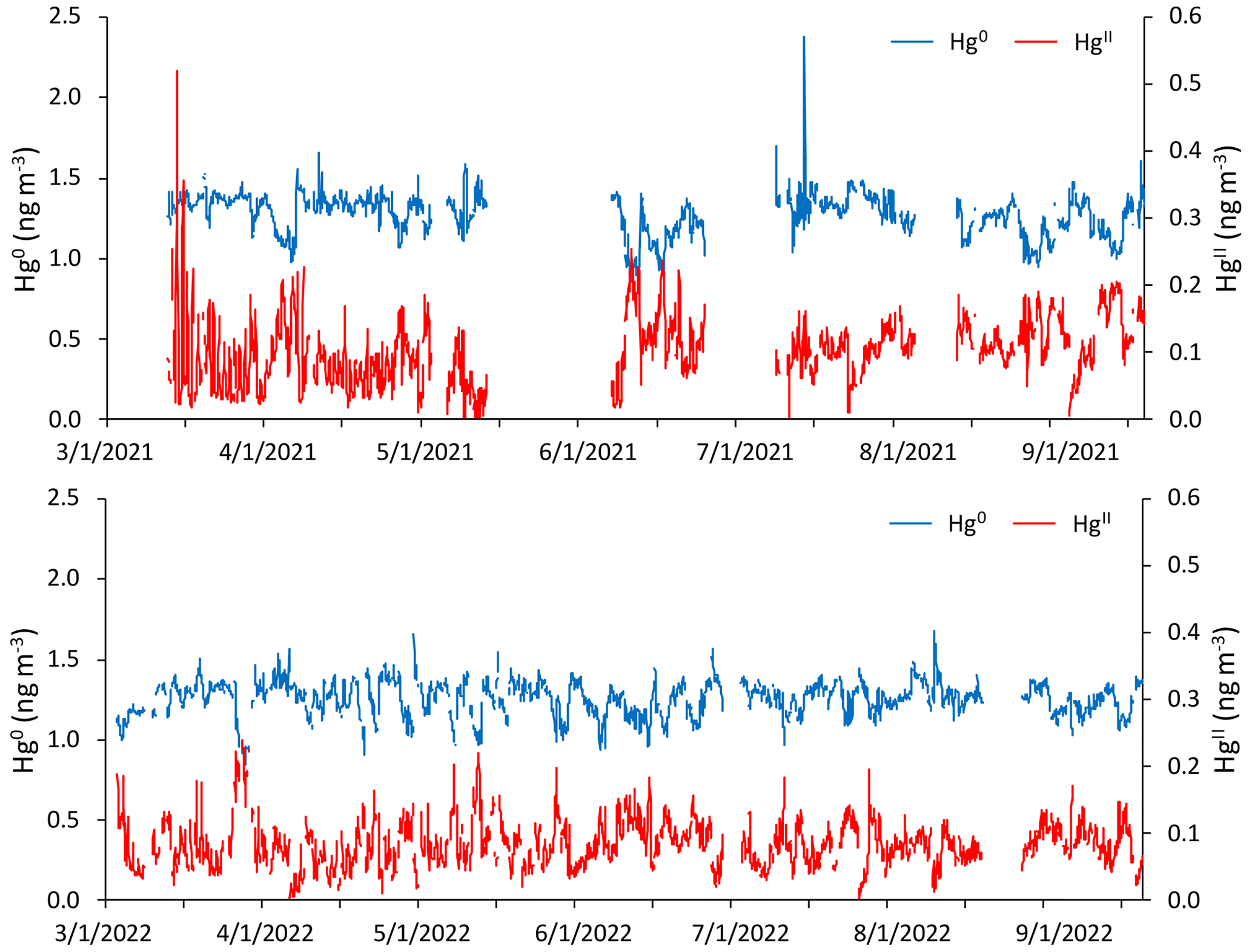
Figure 1Time series of hourly averaged concentrations of Hg0 (blue) and HgII (red) in units of nanograms per cubic meter (ng m−3) between 1 March and 15 September of 2021 and 2022, as measured by the dual-channel system at Storm Peak Laboratory above Steamboat Springs, Colorado. Please note that the date format in this and following figures is month/day/year.
3.1 Data overview
3.1.1 Mercury overview
Figure 1 and Table 1 summarize the hourly averaged measurements of Hg and trace gases from the 2021 and 2022 periods. Overall, mean Hg0 concentrations varied minimally from 2021 (1.27 ± 0.13 ng m−3) to 2022 (1.25 ± 0.11 ng m−3), from spring to summer in each year or from one season to that same season in the following year, even though t tests for comparisons of seasonal means all indicated statistically significant differences (p < 0.01). The largest mean difference in Hg0 was from spring to summer 2021 but was still less than a 0.1 ng m−3 change. Mean HgII concentrations were not significantly different between the two spring seasons (p = 0.33), whereas the summer 2021 mean was significantly higher (p ≪ 0.001) than in summer 2022.
3.1.2 Trace gas overview
Mean values of O3, NOx, CO, and aerosol scattering were significantly different (p < 0.01) between the two spring seasons (excluding CO, which was not available in spring 2021) and between the two summer seasons (Table 1). Mean values were also significantly different between each spring season and the corresponding summer from that year with the exception of NOx in 2022 (p = 0.52). It was notable that O3 displayed a relatively flat diel pattern, with mean diel amplitudes of only 4 ppbv in both spring seasons and 2–3 ppbv in the summer seasons, lacking the pronounced daytime enhancement that is commonly seen at lower-elevation sites (Fig. A2). This behavior was similar to what has been reported at other high-elevation sites that were less influenced by daytime production from local precursor emissions or by nighttime loss processes in the presence of NOx sources (Mueller, 1994; Monks et al., 2000; Bien and Helmig, 2018; Brodin et al., 2010), suggesting that SPL was routinely influenced by the background free troposphere even in the summertime. Higher mean concentrations of O3, NOx, CO, and aerosol scattering in summer 2021 compared to 2022 may be related, at least in part, to observed differences in the frequency of wildfire smoke presence (Sect. 2.3.1).
We also considered the potential influence of the three upwind coal-fired power plants, located 40, 80, and 200 km west of SPL, on Hg concentrations measured at SPL. These plants were shown to influence air mass composition at SPL through emissions of SO2 that can contribute to new particle formation (Hallar et al., 2016). A goal was to determine whether elevated Hg0 or HgII concentrations occurred primarily in the background atmosphere or also under the influence of local or regional point-source emissions. Air masses at SPL were initially defined as power-plant-impacted using the 95th percentile of 10 min averaged SO2 concentrations from the 2021 measurement period. We then examined local wind speed and direction measurements at SPL along with 24 h HYSPLIT back trajectories. We also considered several case studies of the highest SO2 concentrations in each season. Together, these observations showed that higher concentrations of SO2 reliably corresponded to a westerly source region representative of the three upwind power plants. Smoke-impacted periods (Sect. 2.3.1) were excluded from this analysis.
Mean Hg0 and HgII concentrations in spring were statistically significantly different between power-plant-impacted and non-impacted air masses; however, the differences were small enough that we did not consider them to be detectable within instrument precision (Δ mean Hg0 = −0.02 ng m−3, Δ mean HgII = +4 pg m−3). Differences in summertime measurements of Hg0 and HgII between the two types of air masses were also statistically significantly different but only slightly elevated in power-plant-impacted air masses (Δ mean Hg0 = +0.04 ng m−3, Δ mean HgII = +12 pg m−3). Yet, the coefficients of determination between Hg0 and SO2 as well as HgII and SO2 within power-plant-impacted periods were very low in both spring and summer (R2 = 0.00–0.03), indicating that little to no variation in Hg species could be explained by the variability in SO2. We therefore concluded that the three coal-fired power plants upwind of SPL did not significantly contribute to ambient Hg measurements made at SPL. The lack of a measurable enhancement in Hg at the lab when the coal-fired power plant signature was evident can likely be attributed to power plant emissions controls and lower-Hg-content coal (Benson, 2003).
3.1.3 Comparison to similar studies
Mean Hg0 concentrations in this study (1.27 ± 0.13 ng m−3 in 2021 and 1.25 ± 0.11 ng m−3 in 2022) were lower than those reported at other remote mountaintop observatories between 2005–2016, including the Mt. Bachelor Observatory (MBO) in central Oregon, USA (1.54 ± 0.176 ng m−3 from May–August 2005, Swartzendruber et al., 2006); the Lulin Atmospheric Background Station (LABS; 1.73 ng m−3 from April 2006 to December 2007, Sheu et al., 2010); the Pic du Midi Observatory in southern France (PDM; 1.86 ± 0.27 ng m−3 from November 2011–November 2012, Fu et al., 2016); and previously at SPL (1.51 ± 0.11 ng m−3 from October 2006—May 2007, Obrist et al., 2008; 1.6 ± 0.3 ng m−3 from April–July 2008, Faïn et al., 2009). The observed Hg0 means at SPL in 2021 and 2022 were also lower than estimated global background concentrations in the Northern Hemisphere (1.5–1.7 ng m−3; Sprovieri et al., 2016; Mao et al., 2016). One plausible explanation for these differences is the reported declines in ambient Hg0 concentrations in the Northern Hemisphere from the 1990s to 2005–2013, although the magnitudes of reported trends are variable from region to region, ranging from less than 1 % to as much as 3.3 % yr−1 in northern latitude sites (Lyman et al., 2020a, and references therein). Meanwhile Slemr et al. (2011) estimated decreasing trends from 1996 to 2009 of −0.047 (1.4 % yr−1) and −0.035 ± 0.006 (2.7 % yr−1) for the Northern Hemisphere and Southern Hemisphere, respectively. Weigelt et al. (2015) reported a decline of 0.021–0.023 in THg from 1996 to 2013 at the Global Atmosphere Watch (GAW) station in Mace Head, Ireland, one of the longest-running Hg background measurement stations in the Northern Hemisphere. Since the mid-2000s, some studies have reported more modest decreases or even increases in some locations, attributed to variable anthropogenic emission trends and biomass burning, changes in Hg cycling and exchange rates, and the effects of temperature on deposition rates (Lyman et al., 2020a, and references therein). There remain considerable uncertainty and inconsistency in analyses of atmospheric Hg trends, largely because of incomplete emission inventories and a lack of both spatial and long-term measurement coverage (Sonke et al., 2023; Lyman et al., 2020a).
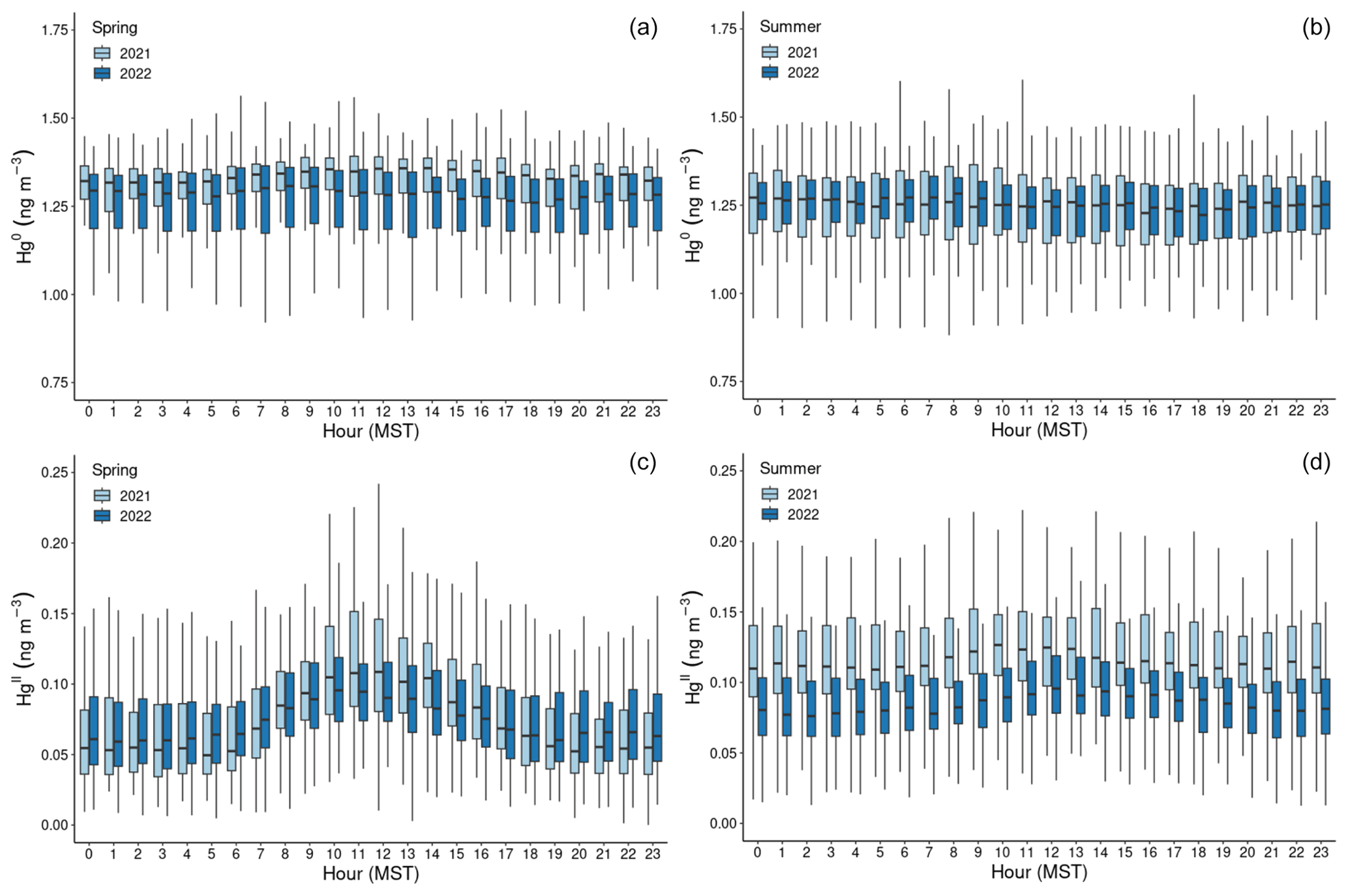
Figure 2Boxplots of concentration measurements by hour of the day (MST) for Hg0 (a, b) and HgII (c, d), showing diel variability during the (a, c) spring and (b, d) summer seasons of the study years. The centerline of each boxplot represents the median concentration, the box represents the interquartile range, and upper (lower) whiskers are either the maximum (minimum) value or the upper-quartile (lower-quartile) value plus (minus) 1.5 times the interquartile range. Outliers are not shown.
Keeping these spatiotemporal trends and sources of uncertainty in mind, we compared the mean Hg0 concentrations at SPL from Obrist et al. (2008) and Faïn et al. (2009) (∼ 1.56 ng m−3) with the mean Hg0 at SPL in 2021 and 2022 (∼ 1.26 ng m−3). Considering this drop of ∼ 0.3 ng m−3 over 14 years, it can be estimated that the more recent measurements were lower by 0.021 (∼ 1.4 % yr−1), values that are within the range of reported downward trends in Northern Hemisphere background concentrations (Slemr et al., 2011; Weigelt et al., 2015; Lyman et al., 2020a; Sonke et al., 2023). Such a difference could also be related to changes in measurement technology between earlier studies and the present one; i.e., gaseous HgII (a.k.a. RGM or GOM) that was not retained on the KCl denuder in the earlier SPL studies may have instead been captured downstream as Hg0, resulting in an overestimate of Hg0 concentrations (Lyman et al., 2010). Even so, total Hg would still have been conserved; yet, the mean (± 1 SD) concentrations of THg were only 1.37 ± 0.11 and 1.34 ± 0.09 ng m−3 in 2021 and 2022, respectively, suggesting that SPL may in fact have experienced declining ambient Hg concentrations over time.
Table 3Event RMA regression slopes ± SE for HgII vs. Hg0; Pearson correlation coefficients for HgII vs. Hg0, RH, O3, and PM1 σsp; and ratios of HgII:Hg0 and HgII:THg.
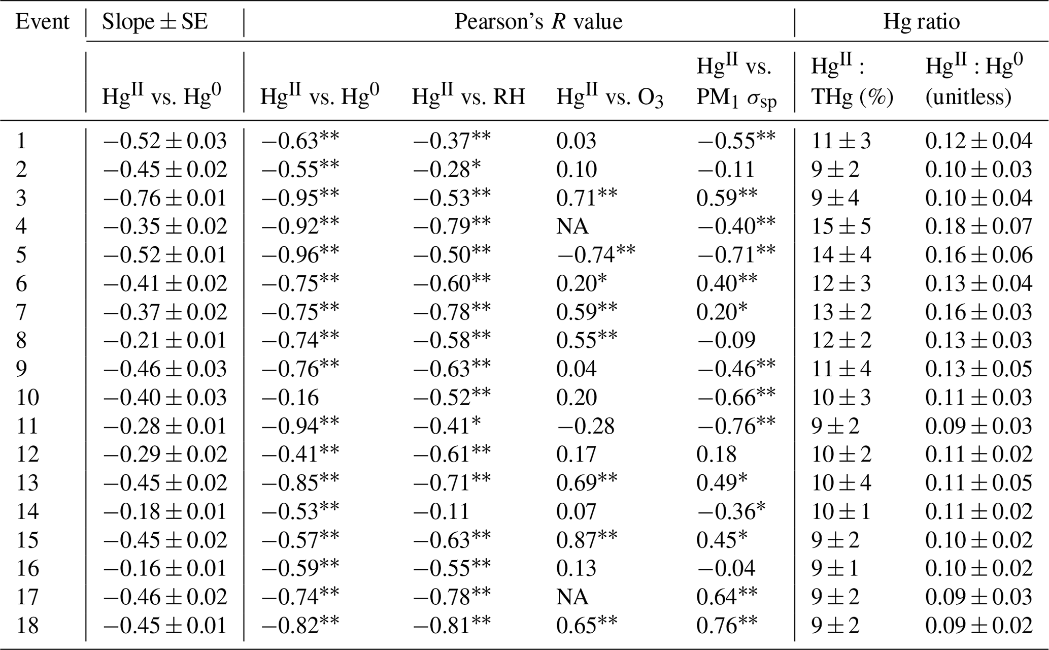
∗ p < 0.05, p < 0.001.
In contrast, concentrations of HgII measured with the dual-channel measurement system in 2021 (103 ± 49 pg m−3) and 2022 (83 ± 35 pg m−3) (Table 1) were considerably higher than the previous measurements made at SPL using the KCl denuder system (Faïn et al., 2009). Summing the April–July 2008 mean measurements of GOM (20 pg m−3) and PBM (9 pg m−3) in Faïn et al. (2009), it can be estimated that the mean HgII during that study period was 29 pg m−3, which is lower than the spring–summer means in 2021 and 2022 by 3.6 and 2.8 times, respectively. The maximum GOM + PBM concentration Faïn et al. (2009) recorded during GOM enhancement events was 159 pg m−3 (Event 4), which is 3.3 times lower than the 2021 maximum (520 pg m−3) and 1.5 times lower than the 2022 maximum (239 pg m−3). Relatedly, mean measurements of GOM and PBM at other mountaintop sites using the KCl denuder system were, respectively, 43 pg m−3 and 5.2 pg m−3 (MBO, USA; Swartzendruber et al., 2006), 12.1 pg m−3 and 2.3 pg m−3 (LABS, Taiwan; Sheu et al., 2010), and 27 pg m−3 and 14 pg m−3 (PDM, France; Fu et al., 2016). While these sites occasionally saw large spikes on the order of hundreds of picograms per cubic meter (pg m−3), it is particularly striking that mean HgII concentrations in the present study were consistently higher than these other sites by a factor of roughly 2 to 5. These observations have important implications for the accurate representation of total Hg speciation in ambient air. For example, estimates of the fraction of atmospheric THg composed of gaseous HgII have ranged from 2 %–20 % depending on sampling location and instrumentation (Dunham-Cheatham et al., 2023; Gustin et al., 2023; Osterwalder et al., 2021; Steffen et al., 2008). During events of elevated HgII in the present study (Sect. 3.2), the maximum percent HgII of THg ranged from 12 %–22 %, with a mean (± SD) of 11 ± 2 %. Comparatively, the previous study at SPL using KCl denuders had a mean HgII:THg ratio during enhanced RGM events of approximately 3 ± 1 % (Faïn et al., 2009). The recent measurements at SPL using the dual-channel system thus represent a significant contribution to the research field in the ability to report verified, accurate, and reliably higher HgII concentration measurements than in past studies.
In both years and for all sampled seasons, Hg0 did not display a pronounced diel pattern (Fig. 2). Elemental Hg generally displayed higher concentrations throughout the day in spring 2021 compared to the same hours in summer 2021 and spring 2022, whereas the spread of data at each hour was larger in summer 2021 and spring 2022. Nevertheless, the diel curves were relatively flat across the hours within all sampled seasons. This finding is in contrast to previous work by Obrist et al. (2008) at SPL, who reported a distinct springtime diel pattern for Hg0. Oxidized Hg, however, displayed markedly higher concentrations during the spring daytime (Fig. 2), with maxima centered around 11:00–12:00 MST and mean diel amplitudes of 58 pg m−3 in spring 2021 and 32 pg m−3 in spring 2022. On a monthly basis (not shown), daytime enhancements were the most pronounced in March 2021, with a mean diel amplitude of 117 pg m−3. In both years, this pattern diminished throughout the spring and into the summer, with mean diel summer amplitudes of 16 pg m−3 (2021) and 19 pg m−3 (2022). The diel curves for HgII also emphasize the overall higher concentrations measured throughout all hours of the day in summer 2021, particularly overnight, as compared to summer 2022 (Fig. 2, Table 1).
Higher daytime concentrations of HgII were also observed at SPL by Faïn et al. (2009). The authors attributed this behavior to surface heating processes and uplift of boundary layer air; however, the daytime maxima during that study tended to occur later in the day, closer to 15:00 MST. In both 2021 and 2022, aerosol PM1 scattering also peaked at midday in spring (Fig. A2), but the amplitude of this enhancement was very small (0.9–2.3 Mm−1). Aerosol PM1 scattering was significantly correlated with HgII in spring 2021, when the daytime enhancement was strongest (R2 = 0.30). These factors could indicate that upslope pollution flow from the local boundary layer contributed to elevated daytime HgII or that the elevated HgII was due to the breakup of the polluted nighttime boundary layer in the Yampa Valley and transport of its pollutants to the site. However, SO2, NOx, O3, and water vapor mixing ratio did not show a notable peak in daytime that would support the notion of transport or mixing from the local boundary layer. If the source of daytime HgII was the breakup of the polluted Yampa Valley boundary layer, it is also not clear why only HgII, and not Hg0, was elevated. In many other studies, urban pollution is associated with Hg0 and not just HgII pollution (Driscoll et al., 2013). The cause of the early spring daytime HgII maximum at SPL thus remains an open question.
The lack of diel variability in Hg0 and a daytime peak in HgII seen in present and past work at SPL is in contrast to other mountaintop studies which reported higher HgII overnight and in the early-morning hours, typically attributed to a shallow planetary boundary layer and subsidence of HgII-rich air from the upper troposphere and lower stratosphere (UT–LS) (Swartzendruber et al., 2006; Sheu et al., 2010; Fu et al., 2016). Nighttime subsidence of HgII from the UT–LS at MBO, PDM, and LABS was also supported by observations of lower RH, higher O3, and air mass back trajectories pointing to upper-tropospheric transport. Further analysis at MBO also identified episodes of high HgII with transport from the marine boundary layer or trans-Pacific transport of combustion emissions from East Asia (Timonen et al., 2013). The more continental nature of SPL is one likely factor that contributed to the different features and transport pathways associated with higher HgII than these other mountaintop sites, as any air masses influenced by the marine boundary layer or trans-Pacific sources may have been diluted by regional continental air masses before reaching the site. Faïn et al. (2009) also showed, and we confirmed in the present work (Sect. 3.2), that high-HgII events at SPL were not associated with UT–LS subsidence and were instead influenced by transport from within the low to middle free troposphere, at least in the 10 d of simulated transport history.
3.2 Multi-day events of enhanced HgII
3.2.1 Behaviors in Hg0, HgII, and atmospheric transport
Based on the criteria described in Sect. 2.3.2, we identified 18 events of enhanced HgII during the 2021 and 2022 measurement periods. Three events occurred during spring 2021, five during summer 2021, two during spring 2022, and eight during summer 2022 (Table 2). Across all events, elevated HgII concentrations were associated with concurrent decreases in Hg0 and RH (Fig. 3). Relative humidity was consistently low during the event periods, with a mean (± SD) event RH of 32 ± 16 %. This observation of high HgII in very dry air masses is consistent with the results of Faïn et al. (2009), who concluded that HgII enhancements at SPL were associated with air masses in the dry (RH < 40 %) free troposphere. In all events but Event 10, HgII was significantly anticorrelated with Hg0 (Pearson's R = −0.95 to −0.41, p < 0.001), and in all events but Event 14, HgII was significantly anticorrelated with RH (Pearson's R = −0.81 to −0.28, p < 0.05). Similar to Faïn et al. (2009), HgII was also anticorrelated with the water vapor mixing ratio during 12 events (Pearson's R = −0.74 to −0.12, p < 0.05). RMA regression slopes (± SE) for HgII vs. Hg0 during each event ranged from −0.76 ± 0.01 to −0.16 ± 0.01 (Table 3), with an average event slope (± SD) of −0.39 ± 0.14. Though previous work at SPL also showed negative RGM–GEM slopes during high-RGM events, the magnitudes were only between −0.07 to −0.18, with an average of −0.10 (Faïn et al., 2009). This difference likely reflects, at least in part, the improved accuracy of the dual-channel system in measuring HgII than previously used instrumentation (Sect. 3.1). The slope of all hourly data during event periods (± SE) in 2021 and 2022 was −0.38 ± 0.09 (Fig. 3).
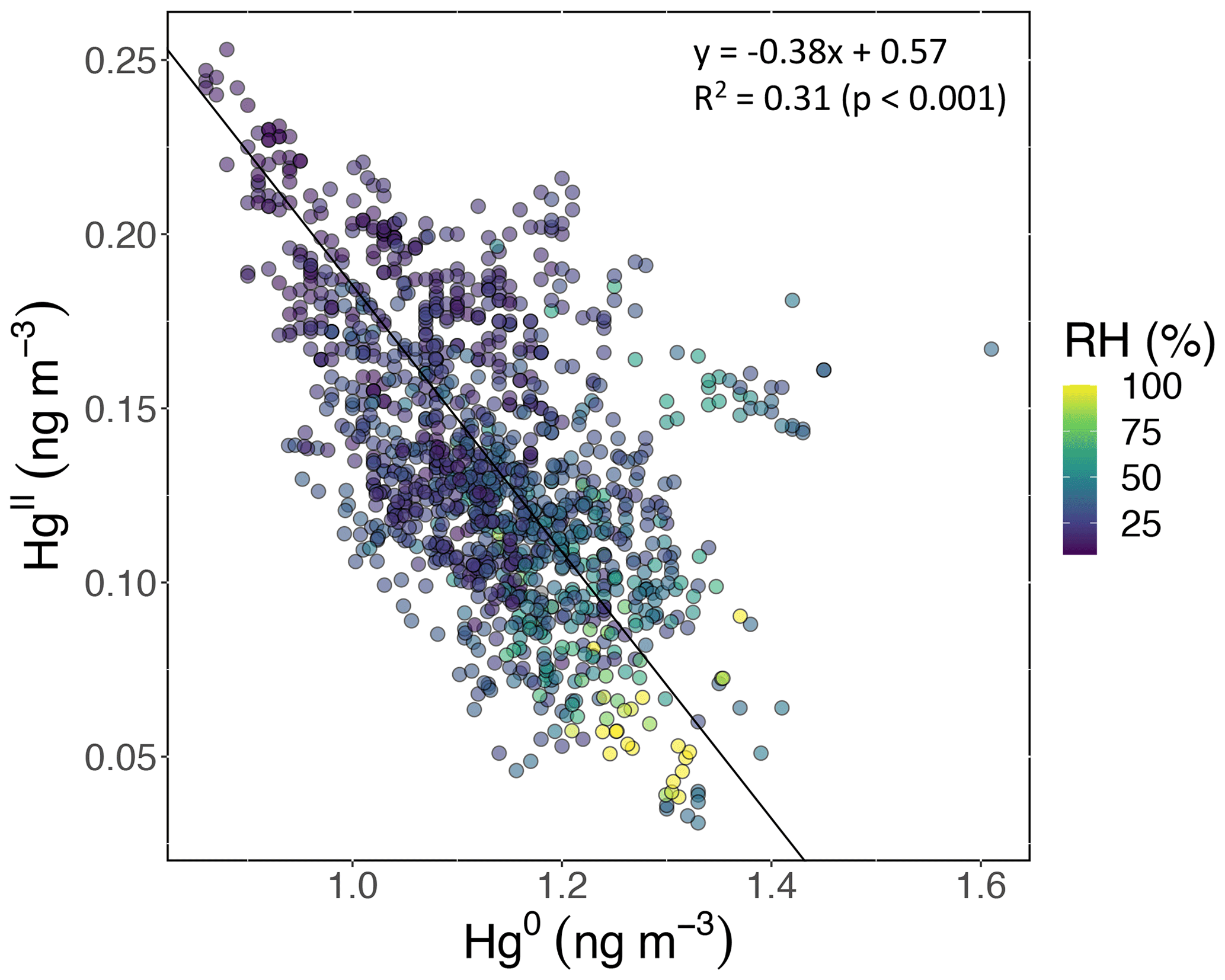
Figure 3HgII vs. Hg0 for hourly measurements during all 18 events, color-coded by RH. HgII was significantly anticorrelated with Hg0 (Pearson's R = −0.55, p ≪ 0.001) and RH (Pearson's R = −0.56, p ≪ 0.001). The slope of the RMA regression (± SE) was −0.38 ± 0.09, which is similar to the average of all 18 event slopes (± SD), which was −0.39 ± 0.14.
By contrast, measurements of enhanced nighttime RGM at MBO during summer 2005 showed a slope nearer to unity for RGM vs. GEM (−0.89) (Swartzendruber et al., 2006). These events, as well as other instances of enhanced RGM at MBO, were hypothesized to have UT–LS influence (Swartzendruber et al., 2006; Timonen et al., 2013). An aircraft study also reported an HgII–Hg0 regression slope for air originating from the upper troposphere that was similarly close to unity (−0.93) and a slope of −0.53 for stratospheric air (Lyman and Jaffe, 2012). The lack of mass closure under stratospheric influence was attributed to the idea that THg decreases toward the stratosphere, while the ratio of HgII:Hg0 simultaneously increases with altitude (Swartzendruber et al., 2006; Lyman and Jaffe, 2012). While a few slopes of individual events in the present study showed values closer to unity (e.g., Event 3 of −0.76 ± 0.01), the total slope of all events was much lower than that seen in air masses influenced by the UT–LS. Meanwhile, Fu et al. (2021) found a slope of −0.44 ± 0.10 for HgII vs. Hg0 during one event of free-tropospheric air mass intrusion at PDM, similar to the mean slope we report here. Unlike the majority of events we identified at SPL, they reported a lack of common air mass origins across their 8 d event, and after correcting for this based on reported latitudinal GEM differences, they obtained a corrected slope of −0.88, implying that most of the HgII was retained within the sampled air masses. Given the relative consistencies in air mass origins (Fig. A3) during our events, the majority of which were 5 d or fewer (Table 2), we did not attempt such a correction.
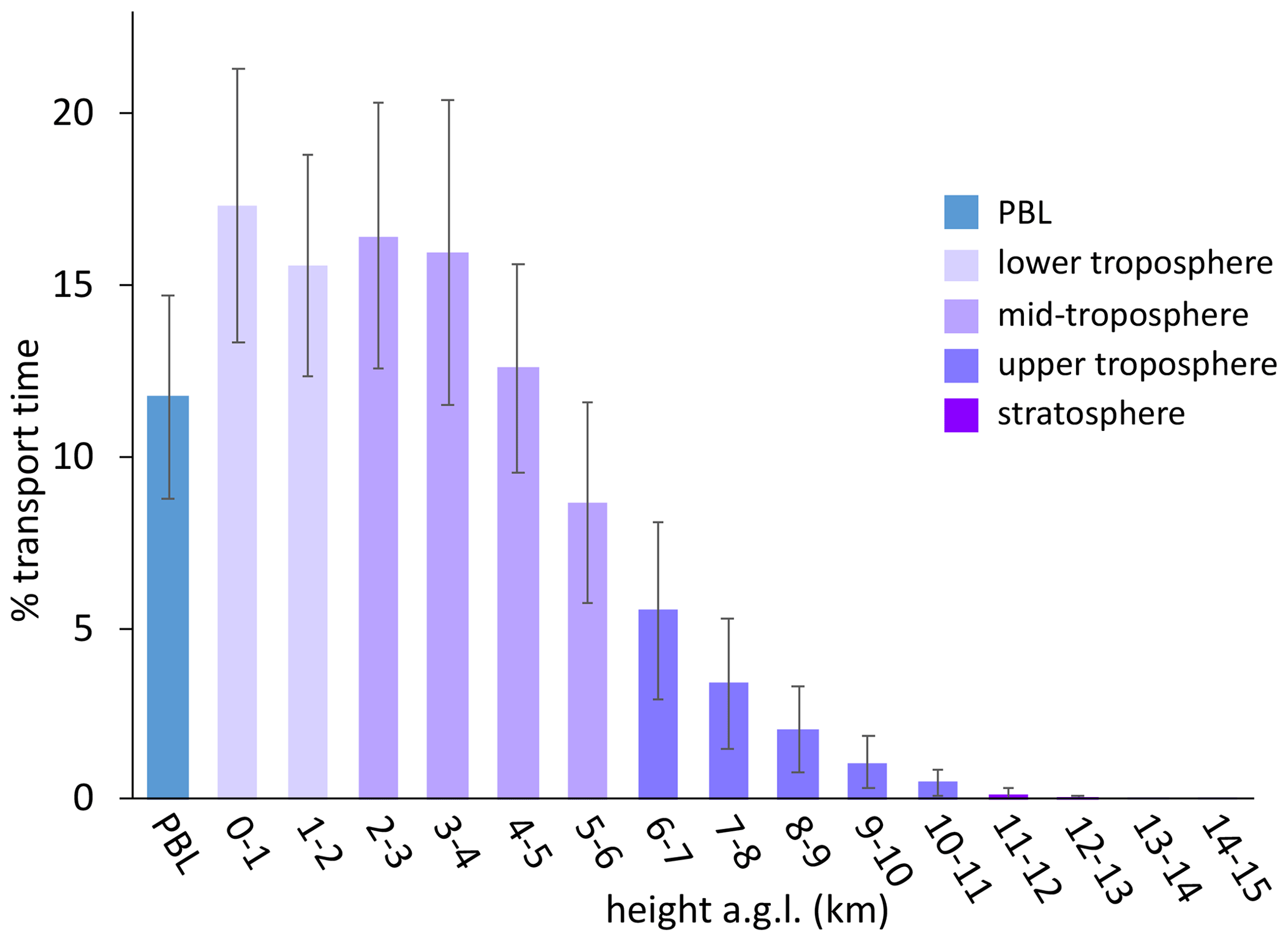
Figure 4The percentage of transport time that high-HgII event air masses spent at each altitude above ground level () averaged across all 18 events. In general, the majority of air mass transport fell in the low to middle altitudes, while the air masses spent less of the transport time within the planetary boundary layer (PBL) or in the upper troposphere and lower stratosphere (UT–LS). Bars are color-coded by layers of the atmosphere. The PBL was explicitly calculated by the HYSPLIT–STILT model, but the other altitude groupings are general approximations.
Instead, we propose that the lack of mass closure may be caused by upwind Hg0 oxidation followed by HgII loss via deposition during transport or scavenging of HgII by cloud droplets (Fu et al., 2021; Lyman and Jaffe, 2012; Swartzendruber et al., 2006), explanations which are further supported by the modeled transport behavior during events at SPL. During all high-HgII events at SPL in 2021 and 2022, the air mass back trajectories generally maintained transport within the low to middle free troposphere over the Pacific Ocean before subsiding over the continent (Fig. A3). The back trajectories from all 18 events spent an average of 12 ± 2 % and a maximum of 16 % of the total transport time in the PBL. Moreover, HYSPLIT–STILT transport analysis showed that event air masses spent on average just 13 ± 5 % (Fig. 4) and a maximum 24 % of transport time above 6 km The median percent transport time spent in the 3–5 km range (chosen here to approximate the low to middle free troposphere) during the events was 43 %. The nine air masses that spent greater than 43 % of their transport at these altitudes had significantly (p < 0.001) higher mean HgII concentrations (142 ± 23 pg m−3) and spent significantly less time in the 0–2 km range (30 ± 3 %) than those that spent less than 43 % of transport in this altitude range (114 ± 11 pg m−3; 38 ± 4 % of transport in the 0–2 km altitude range). The relatively limited influence from both the UT–LS and PBL on the sampled air masses indicated that extended periods of elevated HgII at SPL likely originated in the low to middle free troposphere (Fig. 4). A comparison to transport pathways of air masses associated with low HgII is described in Sect. 3.2.3.
All HYSPLIT–STILT runs demonstrated that SPL experienced prevailing westerlies during the 18 events, as has been demonstrated in earlier work at the site (Faïn et al., 2009; Hallar et al., 2016). However, there was not a consistent directional origin evident by season (Fig. A3) or in relation to covariance in other air mass tracers (Sect. 3.2.2) during high-HgII events. There was also large variability in whether the event air masses originated over the central Pacific, northern Pacific, or southwestern Pacific, as well as the horizontal distance covered in 10 d of transport. Although 10 events showed some or all back trajectories approaching SPL from the southwest, there did not appear to be any consistency in air mass speed, altitude, or composition amongst this subgroup. The horizontal transport pathway alone, therefore, did not appear to directly influence the presence of high concentrations of HgII at SPL.
There was some variation in the amount of time the simulated air masses spent over the North American continent (50 to 150 h of the 10 d transport), but differences were not associated with particular air mass compositions. Simulated air mass temperature was most dependent on season but generally increased over the continent. Additionally, all event back trajectories showed some upwind precipitation during the 10 d but no precipitation within at least 50 h of arrival at SPL. Simulated cloud cover during transport was generally higher (60 %–80 %) upwind of SPL and dropped substantially prior to the end of the trajectories, in most cases reaching near 0 % by arrival at SPL. These indices could account for the lack of mass closure between Hg0 and HgII. Relative humidity remained below 60 % during transport and consistently declined as the air masses approached the site. Therefore, the air masses in which high HgII was measured at the site were generally dry and did not experience significant washout close to the measurement site.
In another study at MBO, maximum RGM : GEM ratios ranged from 0.16 to 1.05 during high-RGM periods, with the largest ratios seen in air masses influenced by the marine boundary layer (MBL) that were marked by circulation above the ocean for at least 10 d prior to arrival at MBO, as well as decreases in CO, aerosol scattering, and O3 (Timonen et al., 2013). These MBL events were associated with higher concentrations of RGM and larger RGM : GEM ratios than seen at SPL (Table 3). By comparison, the mean ratio (SD) of HgII:Hg0 during the 18 events at SPL was 0.12 ± 0.03, and maximum values ranged from 0.13 to 0.29 (a comparison of these values to non-event times will be discussed in Sect. 3.2.3). Mean ratios during summer 2021 Events 4–8 (0.15 ± 0.02) were significantly higher than the rest of the events in the study (0.10 ± 0.01) (p < 0.001), possibly related to mean HgII concentrations being significantly higher in summer 2021 than in other seasons (Sect. 3.1.1). Nevertheless, air masses at SPL did not show behavior or composition comparable to that of MBL-influenced air at MBO. Understandably, by nature of the site locations, the air masses measured at SPL spent much more time over the continent (Fig. A3), potentially allowing for more scavenging of HgII during transport and therefore resulting in HgII–Hg0 regression slopes further from unity and a lower ratio of HgII:Hg0.
In conclusion, based upon the results of the HYSPLIT–STILT and other meteorological analysis, we posit that the lack of mass closure in the slopes of HgII–Hg0 regressions during the 18 events at SPL was likely caused by distant upwind oxidation followed by HgII loss via deposition or cloud droplet uptake during transport. This finding is further supported by the analyses of trace gas measurements and of select non-event periods below.
3.2.2 Event air mass composition
Concentrations and relationships between other trace gases measured in this study varied across the events. Of the 16 events with sufficient O3 measurement coverage, 7 showed significant positive correlations between HgII and O3 (Events 3, 6, 7, 8, 13, 15, and 18), with six of these seven events also having significant positive correlations between HgII and aerosol PM1 scattering (all but Event 8) (Table 3). These events were mostly in summer but occurred in both study years. Event 3 is shown in Appendix A as an example of this type of event (Fig. A4). Ozone concentrations increased by approximately 10 to 20 ppbv during these events, concurrent with fluctuations in HgII concentrations. Meanwhile, the magnitudes of aerosol PM1 scattering enhancements were more varied, ranging from approximately 30 to 120 Mm−1, in part because scattering was generally lower during spring than summer, and some of the summer events also showed evidence of smoke (Sect. 2.3.1).
While Faïn et al. (2009) reported similar transport altitudes for air masses associated with enhanced HgII at SPL, they reported no relationship between HgII and O3. Previous studies at the MBO and PDM mountaintop sites, however, also showed co-enhancements of HgII and O3. Often, these enhancements occurred with simultaneous decreases in Hg0, CO, and aerosol scattering, which Swartzendruber et al. (2006), Timonen et al. (2013), and Fu et al. (2016) attributed to HgII transport from the UT–LS. As previously discussed, however, HYSPLIT–STILT transport analysis during events at SPL did not show air masses at high enough altitudes to indicate UT–LS influence in the 10 d of simulated transport (Fig. A3), and thus we suggest that UT–LS air was not the source of co-enhanced O3 and HgII in these events.
High O3 concentrations could also be generated as a secondary product of natural or anthropogenic combustion. For example, Timonen et al. (2013) reported events of enhanced HgII, O3, aerosol scattering, and CO at MBO during springtime, when meteorological conditions favor long-range trans-Pacific air mass transport and can deliver anthropogenic pollution from the Asian continent (Timonen et al., 2013). Maximum O3 concentrations during the seven events at SPL ranged from 58 to 74 ppbv, values which were comparable to the maximum O3 values reported at MBO during events of high HgII associated with influence from Asian long-range transport, which ranged from 69 to 77 ppbv (Timonen et al., 2013). However, all of the events in this study with positive correlations between HgII and O3 occurred during summertime, with the exception of Event 3 during spring 2021 (Fig. A4). In all cases except for Event 8, back trajectories did not show transport from the Asian continent in the 10 d histories (Fig. A3). Alternatively, O3 could have been picked up from the North American PBL and mixed with free-tropospheric air as the air masses traveled over the continent before arriving at SPL, or O3 could have been produced in conjunction with HgII, as their chemical production mechanisms both involve photochemical processes in dry air conditions.
The enhancement of O3 during some summer events could also be a result of biomass burning, as O3 can be a secondary product in smoke plumes of wildfires (Briggs et al., 2016). Of the 18 events, 8 occurred when SPL was in smoke from local or regional wildfires and experiencing elevated concentrations of combustion tracers, particularly CO and aerosol scattering (Sect. 2.3.1, Table 2). Both O3 and CO were significantly positively correlated with HgII during three events (Events 13, 15, 18), and CO was above 150 ppbv during five events when HgII was significantly correlated with O3 (Events 6, 7, 8, 13, 18). Four events where HgII was correlated with O3 also showed positive correlations between O3 and CO (Events 6–8, 18). Biomass burning has been shown to volatilize stored Hg as Hg0 and release it to the atmosphere. High levels of HgII have not typically been reported in smoke plumes (McLagan et al., 2021; Obrist et al., 2007; Friedli et al., 2003), though all published measurements were collected using denuder-based methods. Elevated HgII concentrations during the events under consideration here, which had concentrations of Hg0 comparable to the seasonal means, may be coincidental to the presence of smoke in the air masses; i.e., it is possible that the smoky air was mixed with cleaner free-tropospheric air containing higher concentrations of HgII. However, it is also possible that co-emitted halogens or aerosols in smoke plumes led to faster oxidation or scavenging of Hg0 than in clean air, leading to elevated HgII and PBM. Further work is needed to characterize the concentrations and chemistry of Hg0 and HgII in smoke plumes using verified measurement methods.
Of the 18 events, 7 showed significant anticorrelations between HgII and PM1 scattering (Events 1, 4, 5, 9, 10, 11, 14; Table 3). Oxidized Hg in these events also tended to be significantly anticorrelated with NOx but not always with other pollution tracers. Three of these events occurred when SPL was in smoke, and therefore PM1 scattering was elevated but showed measurable decreases when HgII increased, indicating that SPL may have experienced some influence from cleaner, free-tropospheric air during these smoky periods. Event 5 (23:00 on 13 June to 21:00 MST on 15 June 2021) (Fig. A5) was the only one of these cases where HgII was significantly anticorrelated with O3 (Pearson's R = −0.74, p < 0.001) and was also anticorrelated with NOx (Pearson's R = −0.43, p < 0.001) and SO2 (Pearson's R = −0.34, p < 0.05). This event also had a particularly strong anticorrelation between HgII and Hg0 (Pearson's R = −0.96, p < 0.001) and RH (Pearson's R = −0.50, p < 0.001) and notably higher-altitude transport than other events (Fig. A5); the air mass spent 23 % of transport time higher than 6 km , compared to an average of 13 ± 5 % for all events. Considering these factors, Event 5 appeared to have particularly clean air conditions, originating from higher in the free troposphere. However, the altitudes associated with Event 5 air mass transport were still not high enough to be considered UT–LS influenced, as the air mass trajectories spent 93 % of transport time below 8 km
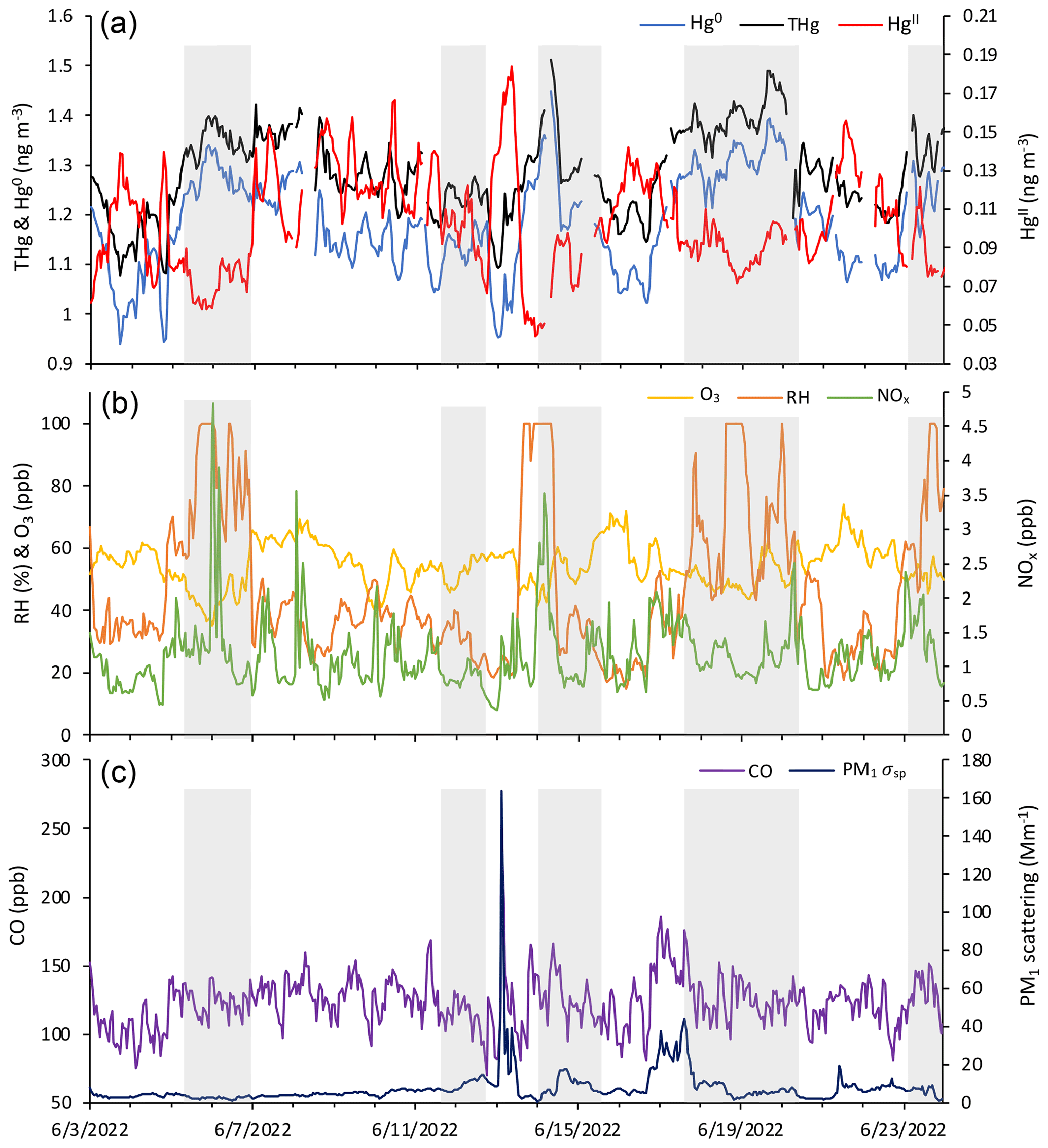
Figure 5Time series of (a) HgII, Hg0, and THg; (b) RH, O3, and NOx; and (c) CO and aerosol PM1 scattering for 04:00 on 3 June to 03:00 MST on 24 June 2022, showing the five events of enhanced HgII that occurred in June 2022 and the five corresponding non-events (shaded in gray).
The occurrence of events with either positive or negative relationships with aerosol scattering could be related to the relative abundance of gaseous vs. particulate HgII (e.g., RGM/GOM vs. PBM). For example, an enhancement in aerosol scattering could indicate a higher proportion of PBM than during other events of elevated HgII, whereas events with lower aerosol scattering could indicate more gaseous HgII. A study at PDM showed that during events of elevated PBM, measured with the Tekran speciation system, aerosol number concentration was significantly anticorrelated with PBM (Fu et al., 2016). The authors posited that this relationship could indicate that atmospheric aerosol concentration may not play a significant role in PBM formation in the middle and upper free troposphere or rather that aerosol number concentration at PDM is driven by anthropogenic influence from the PBL and is therefore not representative of the composition of the middle to upper free troposphere at that site (Fu et al., 2016). However, it is difficult to directly and quantitatively compare aerosol number concentrations reported by Fu et al. (2016) with the aerosol scattering measurements made at SPL, given that scattering is also affected by aerosol size distribution. Moreover, because the dual-channel Hg measurement system does not differentiate between gaseous and particle phases of HgII, any relationship between these variables is speculative at this time.
3.2.3 June 2022 case study
June 2022 contained five distinct events of elevated HgII (Events 11–15), with periods of low HgII in between events (referred to here as “non-events” and numbered 1 through 5) (Fig. 5). The five events during this period had characteristics similar to the other 13 events from this study, such as depleted Hg0 and low RH, but displayed variation in transport pathways, meteorology, and trace gas concentrations. More specifically, all the June 2022 events had strong and significant anticorrelations between HgII and Hg0 (Pearson's R = −0.94 to −0.41, p < 0.001; Table 3), whereas the non-event HgII–Hg0 anticorrelations were either weaker (Non-events 1, 3, and 5) or not significant at the p < 0.05 level (Non-events 2 and 4) (Table A2).
Table 4June 2022 event–non-event mean ± SD for Hg species, THg, RH, PM1 σsp, and trace gases. Bolded values are significantly different at the p < 0.05 level.
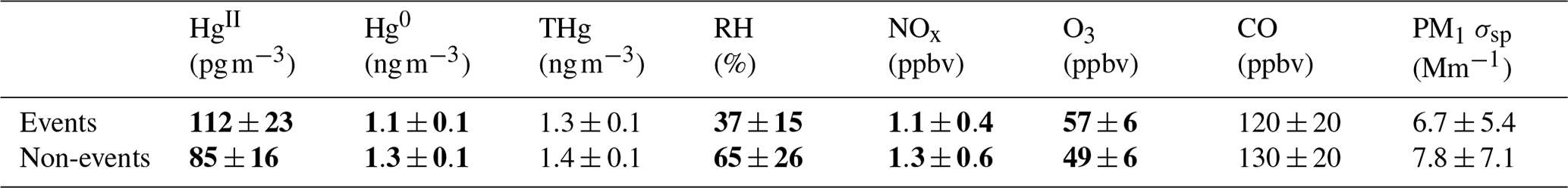
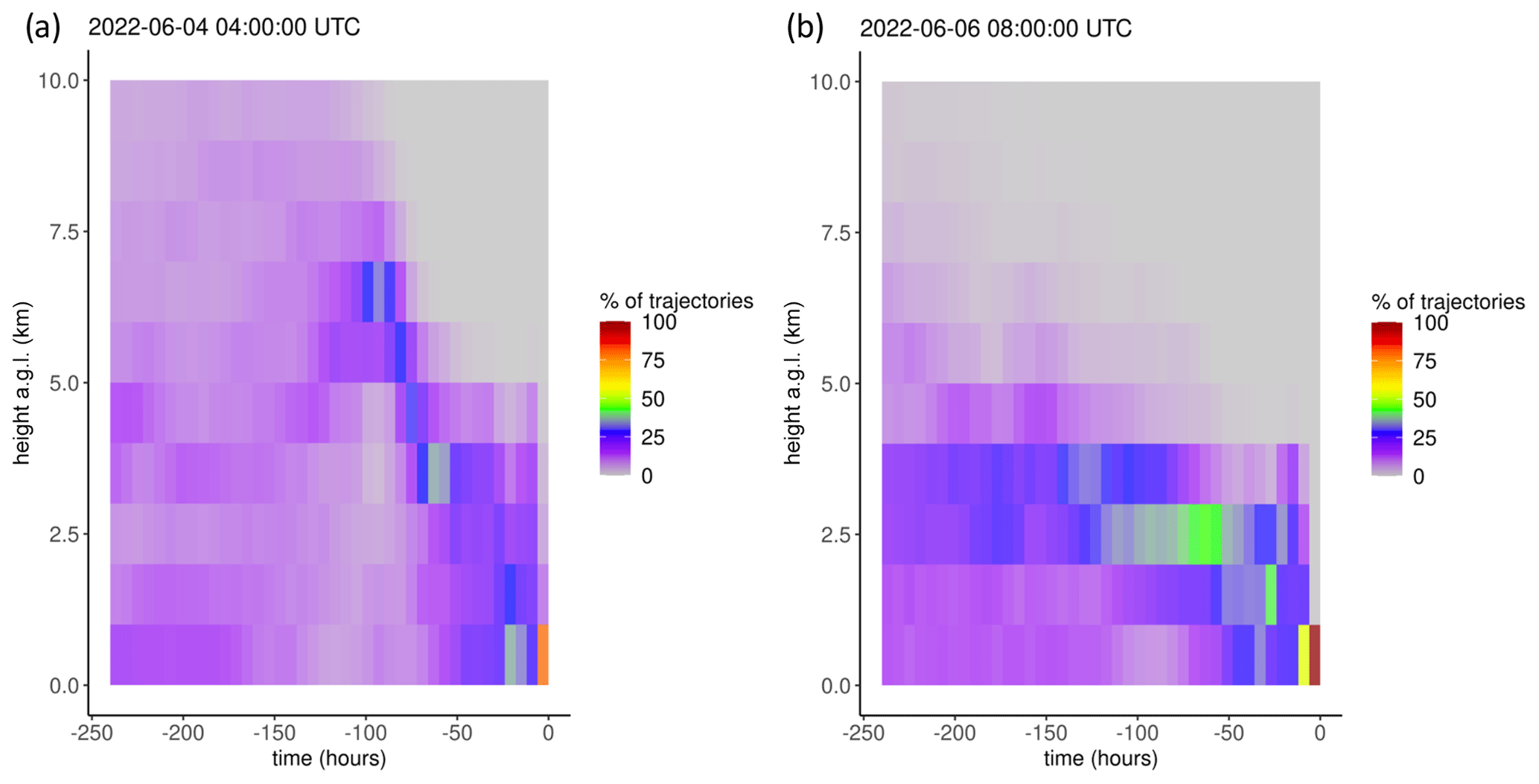
Figure 6Example vertical distributions of air mass trajectories for (a) Event 11 and (b) Non-event 1. Shading reflects the percentage of backward trajectories within a given altitude bin when aggregated to 6 h intervals.
The non-event air masses spent a significantly smaller percentage of transport time in the 3–5 km altitude range (26 ± 4 %) than the event air masses (40 ± 7 %) (p < 0.05) (Fig. A6). Generally, event air masses tended to spend more time at altitudes associated with the low to middle free troposphere, whereas non-event air masses spent more time at lower altitudes and in the PBL (Figs. A6 and A7). June event air masses spent 52 % of transport time above 3 km, whereas non-events spent 44 % of transport time above 3 km. Additionally, the high-HgII events showed significantly higher mean HgII and O3 concentrations and significantly lower mean Hg0, RH, and NOx concentrations than the non-events (Table 4). The ratio of HgII:Hg0 was also significantly higher (p < 0.05) during events (10 ± 1 %) than non-events (6 ± 1 %), and the amount of THg measured as HgII was also significantly (p < 0.001) higher during events (10 ± 1 %) than non-events (7 ± 1 %). Simulated precipitation for the air masses prior to arrival at SPL showed precipitation up to the simulation end time in Non-events 3, 4, and 5. The higher RH during non-event times concurrent with lower HgII concentrations could indicate greater wet deposition or scavenging by clouds of HgII than during event periods. Events 13 and 14 occurred when SPL was influenced by smoke from regional wildfires in Arizona and New Mexico, so both CO and aerosol scattering were elevated (Table 2). Figure 6 shows example transport models for Event 11 (04:00 on 3 June to 04:00 MST on 5 June 2022) and Non-event 1 (05:00 on 5 June to 23:00 MST on 6 June 2022). Event 11 showed higher transport altitudes, lower RH, and no precipitation directly prior to arrival at SPL, whereas Non-event 1 had lower atmospheric transport, higher RH, and more recent precipitation. The differences between event and non-event periods demonstrated that the commonalities in event air mass composition and transport could be attributed to the specific conditions under which Hg oxidation occurred in the upwind atmosphere, as opposed to ambient atmospheric conditions seen locally at SPL.
3.3 Principal component analysis (PCA)
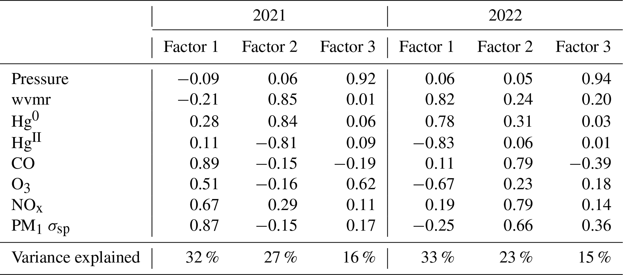
Broadening these event-based analyses to the rest of the hourly measurement data, three factors explaining 60 %–70 % of the total variance were generated in the PCA data reduction technique applied to each of the sampled seasons in 2021 and 2022 (Table B1 and B2) and for the combined 2022 spring–summer period (Table 5). Although differences appeared in the magnitude and sign of variable loadings for each period, there were some notable features that all simulations had in common, as well as some consistent seasonal patterns. For example, all solutions contained two common factors: one representing clean background air with evidence of Hg oxidation (little to no loading of most combustion tracers and inverse loadings of Hg0 and HgII) and another representing anthropogenic and/or biogenic combustion (with some combination of CO, NOx, aerosol scattering, O3, and Hg0 loading having the same sign). In summer 2021 this factor explained the largest percent variance (32 %) and was likely dominated by the aforementioned biomass burning signature, whereas in summer 2022 it explained just 23 % of the variance and likely represented other local regional combustion sources (Tables B1 and B2). The third factor varied in its makeup, but in at least the 2022 applications there were shared loadings of pressure, water vapor mixing ratio, and aerosol scattering and an inverse loading of CO. Another consistent feature was that HgII almost exclusively loaded inversely with Hg0, and on any factor where the two variables did display the same sign, one or both of their loadings were very small (< 0.3). Oxidized Hg was usually but not always inversely related to the water vapor mixing ratio and in some solutions was positively associated with O3 and aerosol scattering but did not load strongly with factors representing combustion sources. These broader features are complementary with the relationships observed during events of high HgII (Sect. 3.2).
Table 5Factor loadings of each variable and the percentage of total variance explained by each factor, as obtained from principal component analysis for the spring–summer 2022 period. wvmr: water vapor mixing ratio.
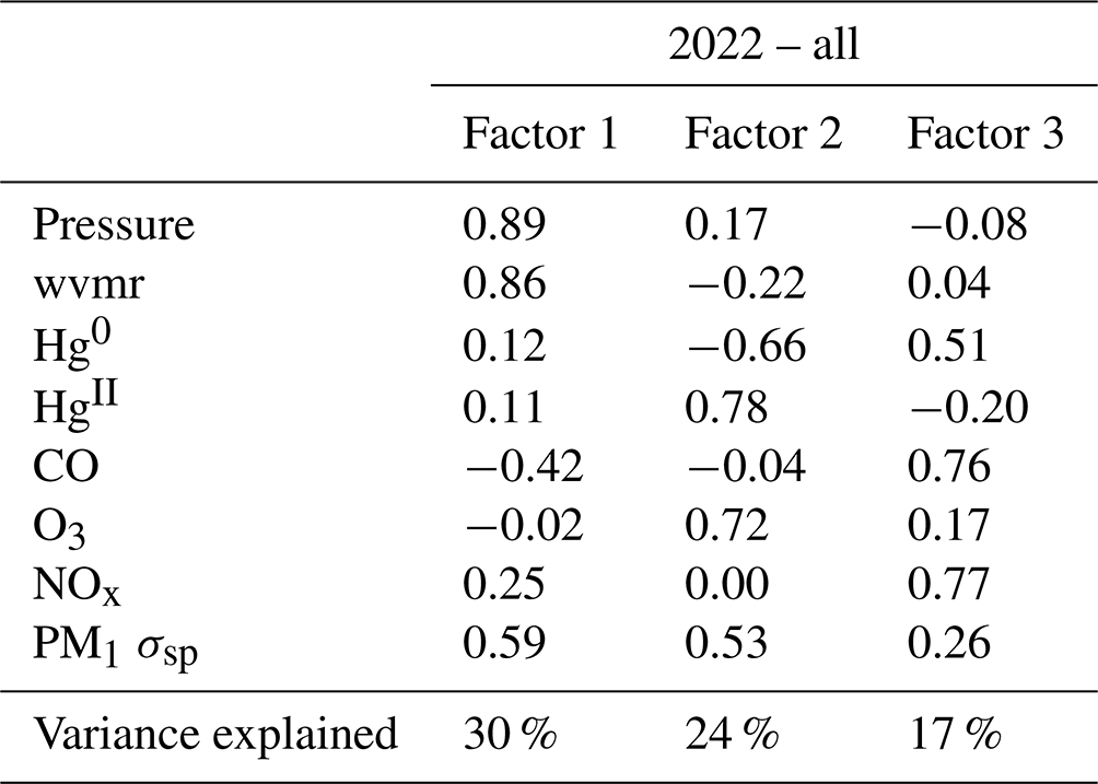
Here we describe the results of PCA application to the combined period of 1 March to 15 September 2022 (Table 5); summaries of the individual spring and summer seasons are provided in Appendix B. Factor 1 (30 %) had strong positive loadings of pressure, water vapor, and aerosol scattering with a moderate negative loading of CO. This factor may represent particle climatology given SPL's history of spending a significant fraction of time in cloud and evidence for new particle formation during particular seasons and times of day (Hallar et al., 2016). Factor 2 (24 % of variance) reflects observations of Hg oxidation within the clean, dry, remote free troposphere. Interestingly, both O3 and aerosol scattering loaded strongly with the same sign as HgII on this factor, a feature that also appeared to some degree in spring 2021 and in the separate analyses of spring 2022 and summer 2022. As shown in Sect. 3.2.2, about one-third of the 18 high-HgII events also had positive correlations for HgII vs. O3 and HgII vs. aerosol scattering. These relationships may point to the potential for Hg oxidation in the presence of O3 but not necessarily in air originating from the UT–LS. This may also suggest the propensity for HgII to be found in the particulate form at SPL in certain instances, but we cannot confirm this due to the current inability of the dual-channel system to distinguish between phases of HgII (e.g., GOM or PBM). Lastly, Factor 3 in 2022 (17 % of variance) represents combustion sources with positive loadings of CO, NOx, and Hg0 with more moderate loadings of O3 and aerosol scattering. It is notable that in the full 2022 analysis, aerosol scattering distributed almost uniformly across all three factors, suggesting multiple drivers for the presence of aerosols at the site that likely vary by season, as evident in the separate spring and summer analyses.
In this study, we examined air mass composition and transport of events of elevated HgII at SPL, a high-elevation mountaintop site, over two 6-month periods in spring and summer 2021 and 2022. Unlike previous studies at mountaintop sites, we employed a dual-channel Hg measurement system, which was calibrated with an SI-traceable calibration system and shown to produce unbiased measurements of HgII (Elgiar et al., 2024). Elemental Hg concentrations and patterns at SPL were similar to those reported in previous work, but mean and maximum HgII concentrations in this study were approximately 3 times higher than earlier measurements at this site, and HgII comprised on average more than 10 % of total atmospheric Hg during high-HgII events. We also demonstrated that Hg concentrations at SPL were not affected by emissions from the three upwind coal-fired power plants, which can likely be attributed to power plant emission controls and lower Hg content in western US coal. Events of elevated HgII showed evidence of upwind Hg0 oxidation, followed by HgII loss during transport in the low to middle free troposphere and no evidence of UT–LS influence. PCA confirmed that HgII measured at SPL was a result of Hg oxidation in the background atmosphere.
Results from this study contribute to the current understanding of Hg oxidation in a remote continental atmosphere. Additionally, the implementation of the dual-channel system provided Hg measurements that were larger in magnitude and more accurate than commercially available instrumentation. Concurrent work related to this project at SPL further elaborates on the methodological improvements for measuring ambient Hg0 and HgII (Elgiar et al., 2024) and the potential contribution of iodine as an emerging Hg oxidant (Lee et al., 2024). Collectively, the results of this campaign will importantly advance the current understanding of ambient Hg origins, cycling, bioavailability, and ultimately ecosystem fate.
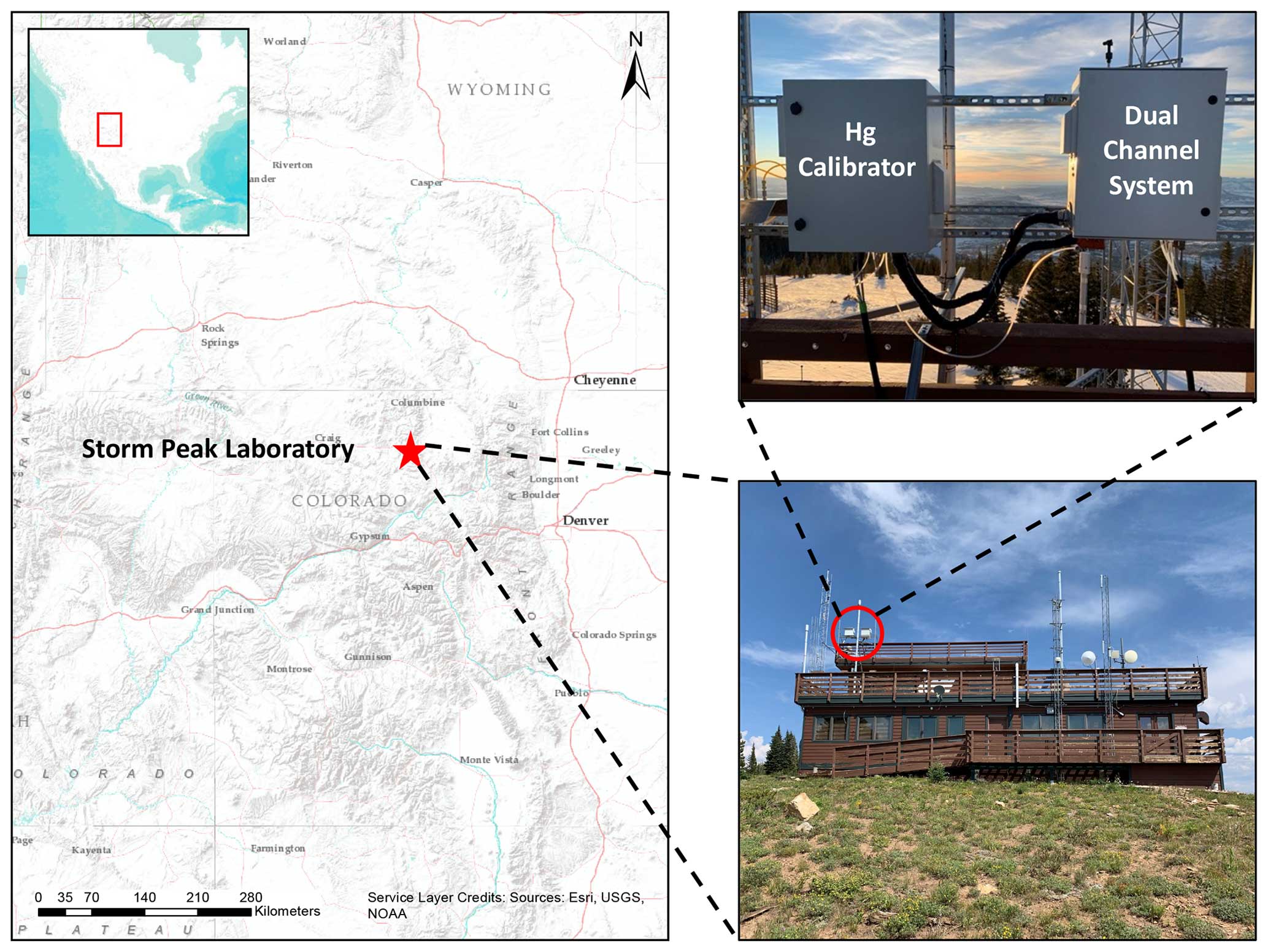
Figure A1Site map of Storm Peak Laboratory and the location of the dual-channel system on the roof of the laboratory (Elgiar et al., 2024).
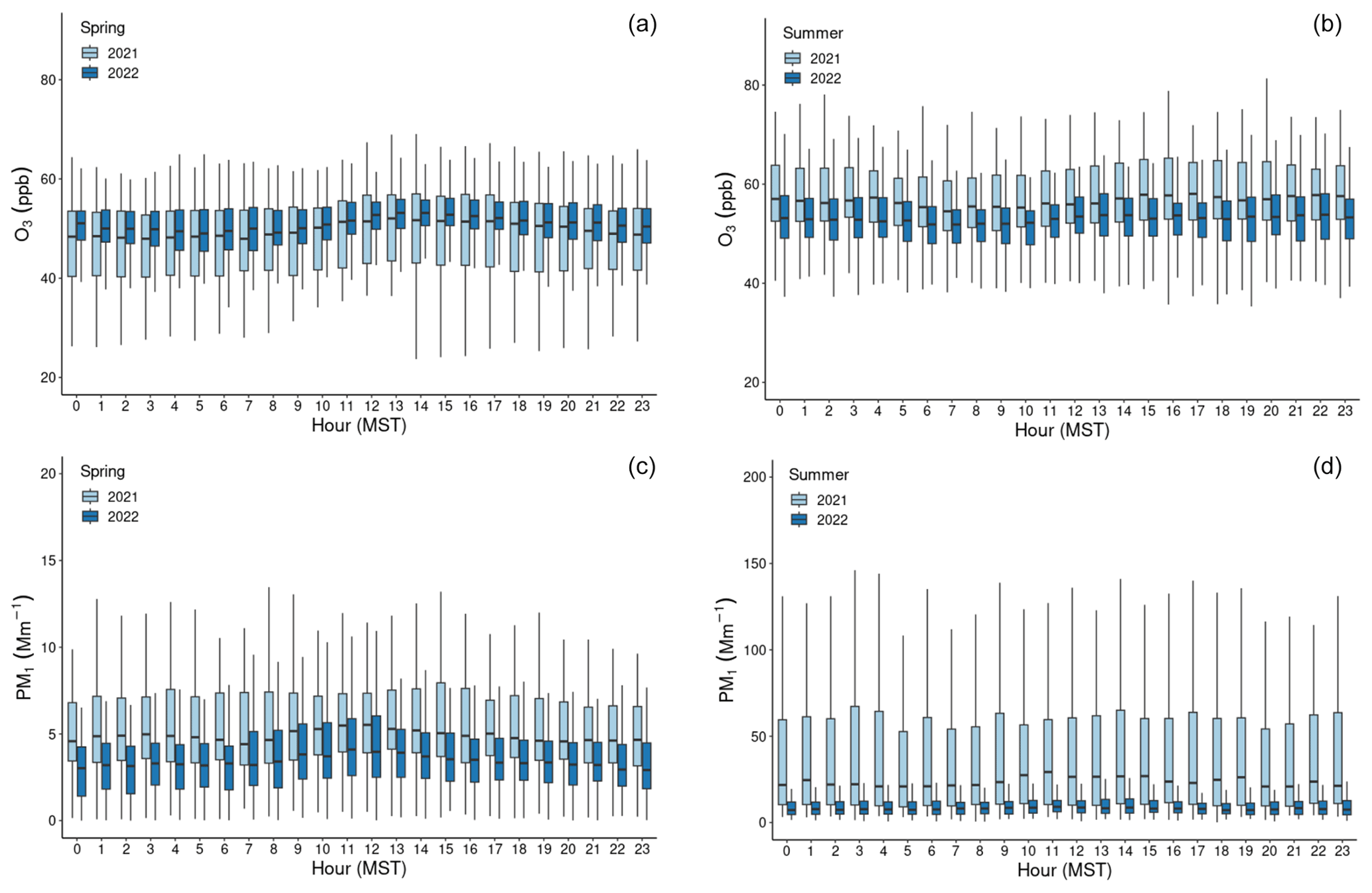
Figure A2Boxplots by hour of the day (MST) for (a, b) O3 and (c, d) PM1 σsp, showing diel variability during the (a, c) spring and (b, d) summer seasons of the study years. The centerline of each boxplot represents the median concentration, the box represents the interquartile range, and upper (lower) whiskers are either the maximum (minimum) value or the upper-quartile (lower-quartile) value plus (minus) 1.5 times the interquartile range. Outliers are not shown.
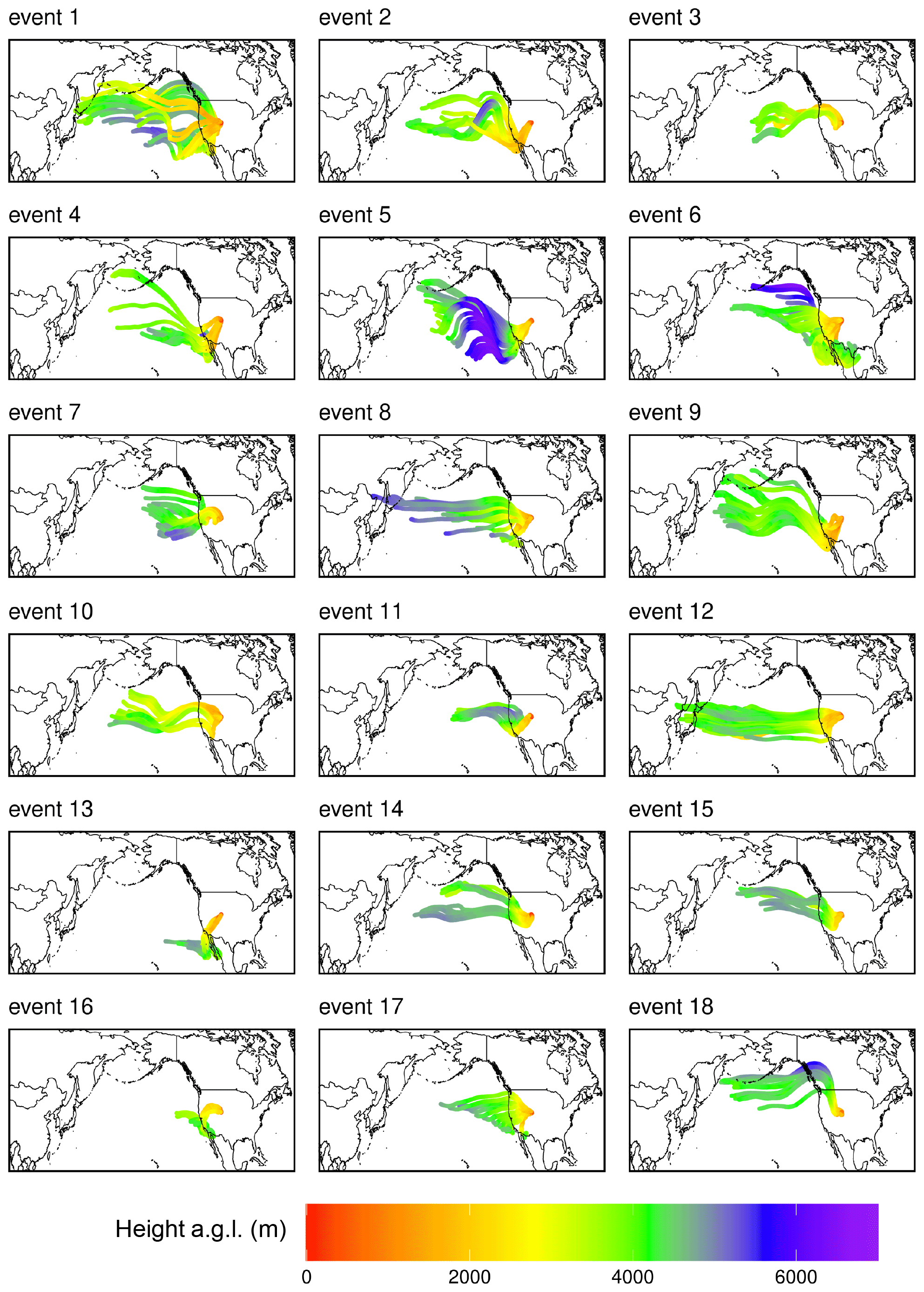
Figure A3Composite maps of averaged HYSPLIT–STILT 10 d back trajectories for all 18 events of elevated HgII, color-coded by altitude above ground level (). Depicted trajectories represent the simulation average transport pathway of 1000 backward trajectories, with simulations initialized at 3 h intervals throughout each event.
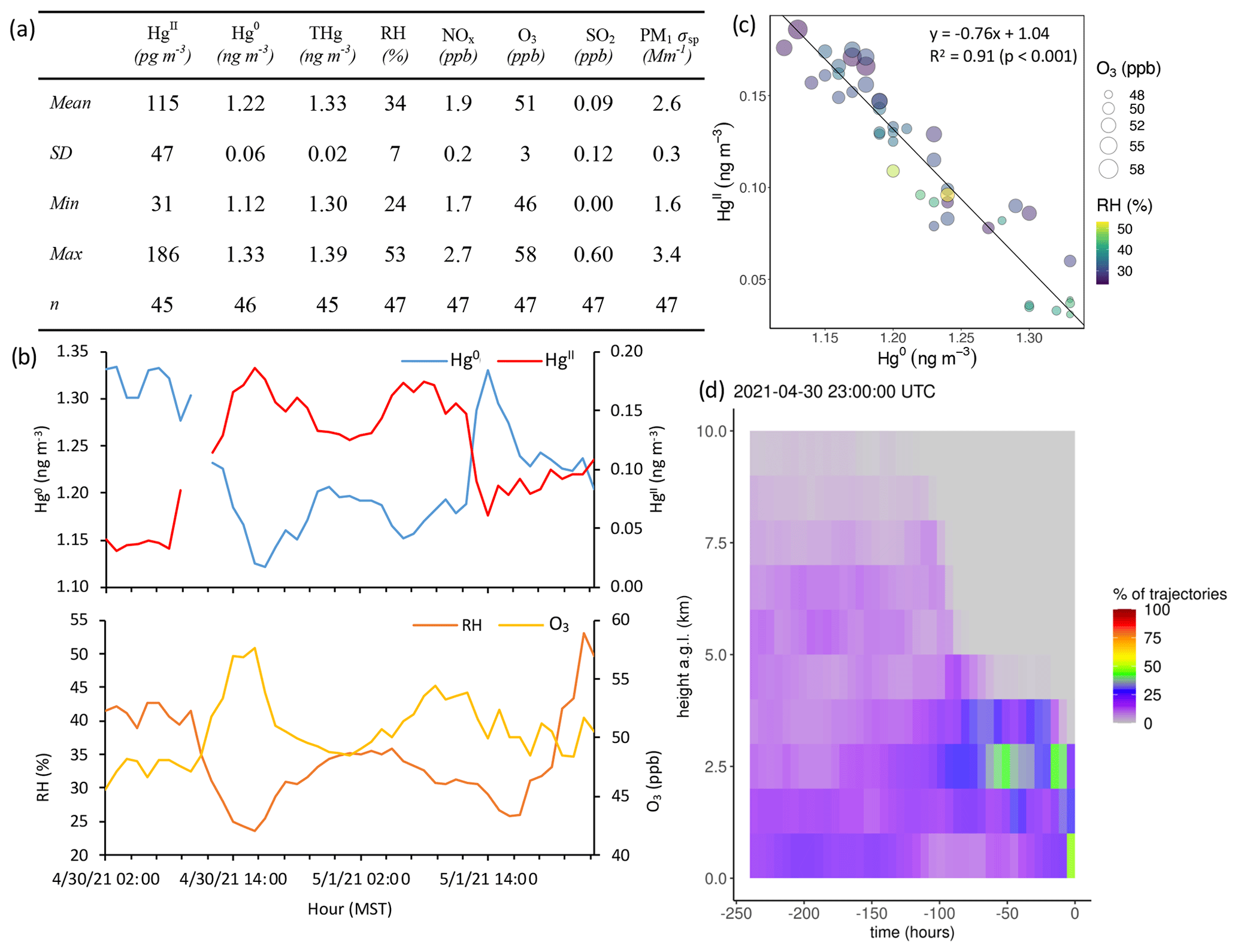
Figure A4Event 3. (a) Descriptive statistics; (b) time series of Hg0, HgII, RH, and O3; (c) scatterplot of HgII vs. Hg0 with RH and O3; and (d) an example vertical profile of HYSPLIT–STILT backward trajectories.
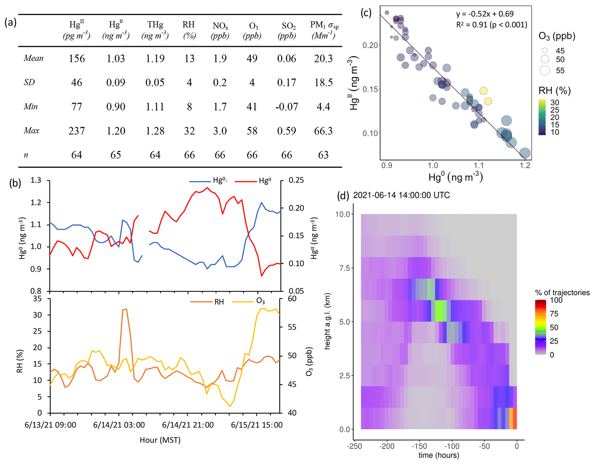
Figure A5Event 5. (a) Descriptive statistics; (b) time series of Hg0, HgII, RH, and O3; (c) scatterplot of HgII vs. Hg0 with RH and O3; and (d) an example vertical profile of HYSPLIT–STILT backward trajectories.
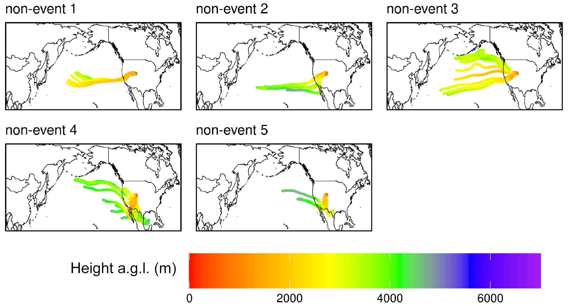
Figure A6Composite maps of averaged HYSPLIT–STILT 10 d back trajectories for the five non-events in the June 2022 case study.
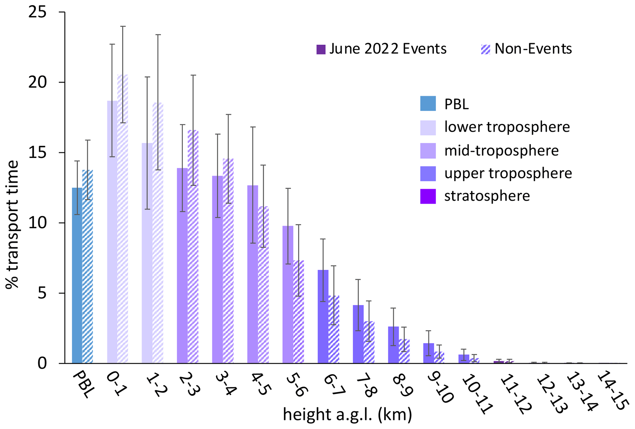
Figure A7The percentage of transport time that high-HgII event air masses spent at each altitude above ground level () averaged for the five June 2022 events and the corresponding June 2022 non-events. Event air masses tended to spend more time at altitudes associated with the low to middle free troposphere, whereas non-event air masses spent more time at lower altitudes and in the PBL. Bars are color-coded by layers of the atmosphere. The PBL was explicitly calculated by the HYSPLIT–STILT model, but the other altitude groupings are general approximations.
Table A1Pearson's correlation coefficients and p values for HgII vs. water vapor mixing ratio (wvmr) for all data in the study period and for all times when relative humidity was below 85 % to limit the analysis to outside of periods when SPL was in cloud. While HgII and wvmr were generally significantly anticorrelated, confirming wvmr as a suitable water vapor metric for PCA, RH had the most robust relationship with HgII, similar to previous studies at SPL (Faïn et al., 2009).
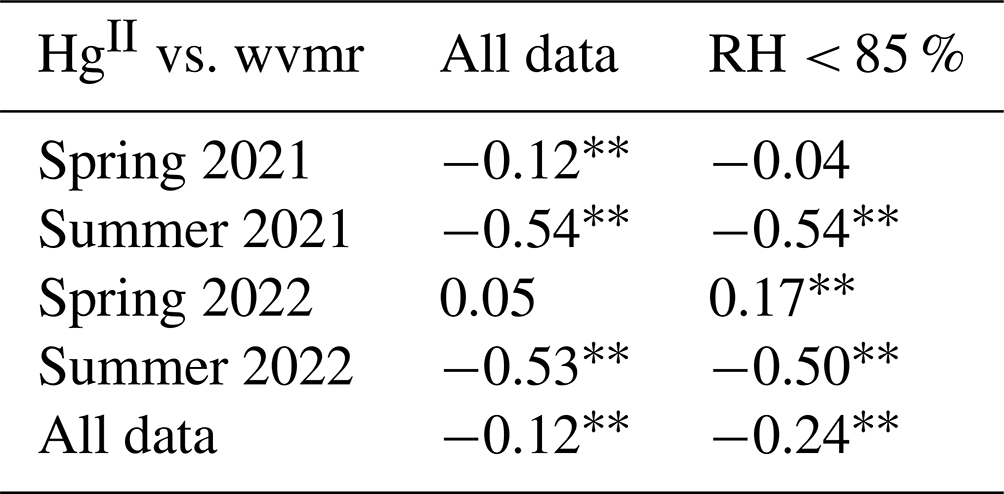
∗ p < 0.05. p < 0.001.
Table A2Pearson correlation coefficients for the five non-events from the June 2022 case study.
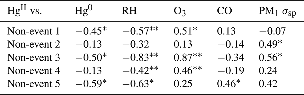
∗ p < 0.05. p < 0.001.
In both spring periods, Factor 1 (27 %–28 % of total variance) was most notably marked by large inverse loadings of Hg0 and HgII. In spring 2021, Factor 1 also had strong loadings of pressure and aerosol scattering of the same sign as HgII, whereas in spring 2022 there were strong loadings of CO and NOx with the opposite sign of HgII. Notably, both Hg0 and HgII distributed strongly on Factors 2 and/or 3 during the spring seasons but always inversely with one another. For HgII, this may be related to the two different temporal patterns driving HgII concentrations in the observations, with a strong diel cycle of high daytime HgII in the early spring (Sect. 3.1), along with the multi-day episodes of high HgII seen throughout the study period (Sect. 3.2). Meanwhile, Hg0 also appeared to be associated with the same sign as combustion tracers such as CO, NOx, and/or O3 as well as with the water vapor mixing ratio (Table B1).
Table B1Factor loadings of each variable and the percentage of total variance explained by each factor, as obtained from principal component analysis for the spring seasons of 2021 and 2022.
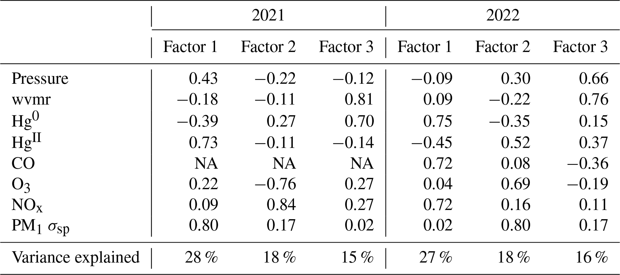
Table B2Factor loadings of each variable and the percentage of total variance explained by each factor, as obtained from principal component analysis for the summer seasons of 2021 and 2022.
The two summer periods showed more consistency between one another in terms of the distributions of variables across different factors. In summer 2021, Factor 1 (32 % of total variance) appeared to represent combustion with strong loadings of the same sign for CO, O3, NOx, and aerosol scattering and a weaker loading of Hg0. A similar factor appeared in summer 2022 but as Factor 2 (23 % of total variance) and with a weaker loading of O3 compared to 2021. The previously mentioned strong influence of local or regional wildfire smoke during at least one-third of the summer 2021 period is likely driving the composition of Factor 1 in summer 2021, while the reduced presence of underlying smoke in summer 2022 but still with the existence of other regional combustion sources likely explains the presence of the combustion fingerprint as Factor 2 in summer 2022. Meanwhile, Factor 2 in 2021 (27 % of variance) and Factor 1 in 2022 (33 % of variance) are consistent with the proposed Hg oxidation in the background dry free troposphere, as indicated by a strong inverse loading of HgII with Hg0 and also a strong inverse loading of HgII with the water vapor mixing ratio, as well as very weak or inverse loadings of combustion tracers such as CO or NOx. Interestingly, in summer 2022 this factor also had a strong loading of O3 and a weak loading of aerosol scattering, both with the same sign as HgII, but this was much less evident in summer 2021 (Table B2).
Ambient air data collected during this project are publicly available at https://doi.org/10.5281/zenodo.10699270 (Gratz et al., 2024).
LEG, SNL, AGH, and RV planned the campaign; TRE, SNL, LEG, AGH, and NSH collected the measurements; SNL and TRE developed and improved the dual-channel Hg measurement system; EJD, LEG, TRE, and NWH analyzed the data; JCL developed and TYW ran the HYSPLIT–STILT model; EJD and LEG wrote the manuscript; and SNL, AGH, RV, TYW, CFL, PWP, NWH, JCL, TRE, and NSH reviewed and edited the manuscript.
The contact author has declared that none of the authors has any competing interests.
Publisher's note: Copernicus Publications remains neutral with regard to jurisdictional claims made in the text, published maps, institutional affiliations, or any other geographical representation in this paper. While Copernicus Publications makes every effort to include appropriate place names, the final responsibility lies with the authors.
Funding for this work was provided by the National Science Foundation (NSF) (award nos. 1951513, 1951514, 1951515, and 1951632). The authors thank Ian McCubbin, Dan Gilchrist, and Maria Garcia for assisting with instrument maintenance and data acquisition; Betsy Andrews of NOAA ESRL GML for providing aerosol data; and Megan Ostlie for working up the trace gas data. Colorado College undergraduate students Brandon Chan and Zoe Zwecker contributed to the preliminary data analyses related to the results presented in this paper.
This research has been supported by the Directorate for Geosciences Division of Atmospheric and Geospace Sciences (grant nos. 1951513, 1951514, 1951515, and 1951632).
This paper was edited by Aurélien Dommergue and reviewed by two anonymous referees.
AirNow-Tech: Navigator, https://www.airnowtech.org/navigator/ (last access: 25 October 2023), 2023.
Andrews, E., Sheridan, P. J., Ogren, J. A., Hageman, D., Jefferson, A., Wendell, J., Alástuey, A., Alados-Arboledas, L., Bergin, M., Ealo, M., Hallar, A. G., Hoffer, A., Kalapov, I., Keywood, M., Kim, J., Kim, S.-W., Kolonjari, F., Labuschagne, C., Lin, N.-H., Macdonald, A., Mayol-Bracero, O. L., McCubbin, I. B., Pandolfi, M., Reisen, F., Sharma, S., Sherman, J. P., Sorribas, M., and Sun, J.: Overview of the NOAA/ESRL Federated Aerosol Network, B. Am. Meteorol. Soc., 100, 123–135, https://doi.org/10.1175/BAMS-D-17-0175.1, 2019.
Ayers, G. P.: Comment on regression analysis of air quality data, Atmos. Environ., 35, 2423–2425, https://doi.org/10.1016/S1352-2310(00)00527-6, 2001.
Benson, S. A.: How does Western coal affect mercury emissions?, EM-Environmental Manager, 32–34, 2003.
Bien, T. and Helmig, D.: Changes in summertime ozone in Colorado during 2000–2015, Elementa: Science of the Anthropocene, 6, 55, https://doi.org/10.1525/elementa.300, 2018.
Bishop, K., Shanley, J. B., Riscassi, A., de Wit, H. A., Eklöf, K., Meng, B., Mitchell, C., Osterwalder, S., Schuster, P. F., Webster, J., and Zhu, W.: Recent advances in understanding and measurement of mercury in the environment: Terrestrial Hg cycling, Sci. Total Environ., 721, 137–647, https://doi.org/10.1016/j.scitotenv.2020.137647, 2020.
Briggs, N. L., Jaffe, D. A., Gao, H., Hee, J. R., Baylon, P. M., Zhang, Q., Zhou, S., Collier, S. C., Sampson, P. D., and Cary, R. A.: Particulate Matter, Ozone, and Nitrogen Species in Aged Wildfire Plumes Observed at the Mount Bachelor Observatory, Aerosol Air Qual. Res., 16, 3075–3087, https://doi.org/10.4209/aaqr.2016.03.0120, 2016.
Brodin, M., Helmig, D., and Oltmans, S.: Seasonal ozone behavior along an elevation gradient in the Colorado Front Range Mountains, Atmos. Environ., 44, 5305–5315, https://doi.org/10.1016/j.atmosenv.2010.06.033, 2010.
Brown, R. J., Brown, A. S., Yardley, R. E., Corns, W. T., Stockwell, P. B.: A practical uncertainty budget for ambient mercury vapour measurement, Atmos. Environ., 42, 2504–2517, https://doi.org/10.1016/j.atmosenv.2007.12.012, 2008.
Castro, P. J., Kellö, V., Cernušák, I., and Dibble, T. S.: Together, Not Separately, OH and O3 Oxidize Hg(0) to Hg(II) in the Atmosphere, J. Phys. Chem. A, 126, 8266–8279, https://doi.org/10.1021/acs.jpca.2c04364, 2022.
Coburn, S., Dix, B., Edgerton, E., Holmes, C. D., Kinnison, D., Liang, Q., ter Schure, A., Wang, S., and Volkamer, R.: Mercury oxidation from bromine chemistry in the free troposphere over the southeastern US, Atmos. Chem. Phys., 16, 3743–3760, https://doi.org/10.5194/acp-16-3743-2016, 2016.
Collaud Coen, M., Andrews, E., Aliaga, D., Andrade, M., Angelov, H., Bukowiecki, N., Ealo, M., Fialho, P., Flentje, H., Hallar, A. G., Hooda, R., Kalapov, I., Krejci, R., Lin, N.-H., Marinoni, A., Ming, J., Nguyen, N. A., Pandolfi, M., Pont, V., Ries, L., Rodríguez, S., Schauer, G., Sellegri, K., Sharma, S., Sun, J., Tunved, P., Velasquez, P., and Ruffieux, D.: Identification of topographic features influencing aerosol observations at high altitude stations, Atmos. Chem. Phys., 18, 12289–12313, https://doi.org/10.5194/acp-18-12289-2018, 2018.
Custódio, D., Pfaffhuber, K. A., Spain, T. G., Pankratov, F. F., Strigunova, I., Molepo, K., Skov, H., Bieser, J., and Ebinghaus, R.: Odds and ends of atmospheric mercury in Europe and over the North Atlantic Ocean: temporal trends of 25 years of measurements, Atmos. Chem. Phys., 22, 3827–3840, https://doi.org/10.5194/acp-22-3827-2022, 2022.
de Krom, I., Bavius, W., Ziel, R., Efremov, E., van Meer, D., van Otterloo, P., van Andel, I., van Osselen, D., Heemskerk, M., van der Veen, A. M. H., Dexter, M. A., Corns, W. T., and Ent, H.: Primary mercury gas standard for the calibration of mercury measurements, Measurement, 169, 108351, https://doi.org/10.1016/j.measurement.2020.108351, 2021.
Dibble, T. S., Tetu, H. L., Jiao, Y., Thackray, C. P., and Jacob, D. J.: Modeling the OH-Initiated Oxidation of Mercury in the Global Atmosphere without Violating Physical Laws, J. Phys. Chem. A, 124, 444–453, https://doi.org/10.1021/acs.jpca.9b10121, 2020.
Dowell, D. C., Alexander, C. R., James, E. P., Weygandt, S. S., Benjamin, S. G., Manikin, G. S., Blake, B. T., Brown, J. M., Olson, J. B., Hu, M., Smirnova, T. G., Ladwig, T., Kenyon, J. S., Ahmadov, R., Turner, D. D., Duda, J. D., and Alcott, T. I.: The High-Resolution Rapid Refresh (HRRR): An Hourly Updating Convection-Allowing Forecast Model. Part I: Motivation and System Description, Weather Forecast., 37, 1371–1395, https://doi.org/10.1175/WAF-D-21-0151.1, 2022.
Driscoll, C. T., Mason, R. P., Chan, H. M., Jacob, D. J., and Pirrone, N.: Mercury as a Global Pollutant: Sources, Pathways, and Effects, Environ. Sci. Technol.,, 47, 4967–4983, https://doi.org/10.1021/es305071v, 2013.
Dunham-Cheatham, S. M., Lyman, S., and Gustin, M. S.: Comparison and calibration of methods for ambient reactive mercury quantification, Sci. Total Environ., 856, 159–219, https://doi.org/10.1016/j.scitotenv.2022.159219, 2023.
Elgiar, T. R., Lyman, S. N., Andron, T. D., Gratz, L. E., Hallar, A. G., Horvat, M., Nair, S. V., O'Neil, T., Volkamer, R., and Živković, I.: Traceable Calibration of Atmospheric Oxidized Mercury Measurements, Environ. Sci. Technol.,, 58, 10706–10716, https://doi.org/10.1021/acs.est.4c02209, 2024.
Faïn, X., Obrist, D., Hallar, A. G., Mccubbin, I., and Rahn, T.: High levels of reactive gaseous mercury observed at a high elevation research laboratory in the Rocky Mountains, Atmos. Chem. Phys., 9, 8049–8060, https://doi.org/10.5194/acp-9-8049-2009, 2009.
Friedli, H. R., Radke, L. F., Lu, J. Y., Banic, C. M., Leaitch, W. R., and MacPherson, J. I.: Mercury emissions from burning of biomass from temperate North American forests: laboratory and airborne measurements, Atmos. Environ., 37, 253–267, https://doi.org/10.1016/S1352-2310(02)00819-1, 2003.
Fu, X., Marusczak, N., Heimbürger, L.-E., Sauvage, B., Gheusi, F., Prestbo, E. M., and Sonke, J. E.: Atmospheric mercury speciation dynamics at the high-altitude Pic du Midi Observatory, southern France, Atmos. Chem. Phys., 16, 5623–5639, https://doi.org/10.5194/acp-16-5623-2016, 2016.
Fu, X., Jiskra, M., Yang, X., Marusczak, N., Enrico, M., Chmeleff, J., Heimbürger-Boavida, L.-E., Gheusi, F., and Sonke. J. E.: Mass-Independent Fractionation of Even and Odd Mercury Isotopes during Atmospheric Mercury Redox Reactions, Environ. Sci. Technol.,, 55, 10164–10174, https://doi.org/10.1021/acs.est.1c02568, 2021.
Gkatzelis, G. I., Coggon, M. M., McDonald, B. C., Peischl, J., Gilman, J. B., Aikin, K. C., Robinson, M. A., Canonaco, F., Prevot, A. S. H., Trainer, M., and Warneke, C.: Observations Confirm that Volatile Chemical Products Are a Major Source of Petrochemical Emissions in U. S. Cities, Environ. Sci. Technol.,, 55, 4332–4343, https://doi.org/10.1021/acs.est.0c05471, 2021.
Gratz, L. E., Ambrose, J. L., Jaffe, D. A., Shah, V., Jaeglé, L., Stutz, J., Festa, J., Spolaor, M., Tsai, C., Selin, N. E., Song, S., Zhou, X., Weinheimer, A. J., Knapp, D. J., Montzka, D. D., Flocke, F. M., Campos, T. L., Apel, E., Hornbrook, R., Blake, N. J., Hall, S., Tyndall, G. S., Reeves, M., Stechman, D., and Stell, M.: Oxidation of mercury by bromine in the subtropical Pacific free troposphere, Geophys. Res. Lett., 42, https://doi.org/10.1002/2015GL066645, 2015.
Gratz, L., Lyman, S., Elgiar, T., and Hallar, A. G.: Measurements of atmospheric mercury, trace gases, aerosols, and meteorology at Storm Peak Laboratory, Colorado, in 2021 and 2022, Zenodo [data set], https://doi.org/10.5281/zenodo.10699270, 2024.
Gustin, M. S., Amos, H. M., Huang, J., Miller, M. B., and Heidecorn, K.: Measuring and modeling mercury in the atmosphere: a critical review, Atmos. Chem. Phys., 15, 5697–5713, https://doi.org/10.5194/acp-15-5697-2015, 2015.
Gustin, M. S., Dunham-Cheatham, S. M., Choma, N., Shoemaker, K. T., and Allen, N.: Determining sources of reactive mercury compounds in Reno, Nevada, United States, Front. Environ. Chem., 4, 1202957, https://doi.org/10.3389/fenvc.2023.1202957, 2023.
Gustin, M. S., Dunham-Cheatham, S. M., Lyman, S., Horvat, M., Gay, D. A., Gačnik, J., Gratz, L., Kempkes, G., Khalizov, A., Lin, C.-J., Lindberg, S., Lown, L., Martin, L., Mason, R., MacSween, K., Nair, S., Nguyen, L. S. P., O'Neil, T., Sommar, J., Weiss-Penzias, P., Zhang, L., and Živković, I.: Measurement of Atmospheric Mercury: Current Limitations and Suggestions for Improvements, Environ. Sci. Technol.,, https://doi.org/10.1021/acs.est.4c06011, 2024.
Hallar, A. G., Petersen, R., McCubbin, I. B., Lowenthal, D., Lee, S., Andrews, E., and Yu, F.: Climatology of New Particle Formation and Corresponding Precursors at Storm Peak Laboratory, Aerosol Air Qual. Res., 16, 816–826, https://doi.org/10.4209/aaqr.2015.05.0341, 2016.
Hopke, P. K. and Jaffe, D. A.: Letter to the Editor: Ending the Use of Obsolete Data Analysis Methods, Aerosol Air Qual. Res., 20, 688–689, https://doi.org/10.4209/aaqr.2020.01.0001, 2020.
Jaffe, D. A., Lyman, S., Amos, H. M., Gustin, M. S., Huang, J., Selin, N. E., Levin, L., Ter Schure, A., Mason, R. P., Talbot, R., Rutter, A., Finley, B., Jaeglé, L., Shah, V., McClure, C., Ambrose, J., Gratz, L., Lindberg, S., Weiss-Penzias, P., Sheu, G.-R., Feddersen, D., Horvat, M., Dastoor, A., Hynes, A. J., Mao, H., Sonke, J. E., Slemr, F., Fisher, J. A., Ebinghaus, R., Zhang, Y., and Edwards, G.: Progress on Understanding Atmospheric Mercury Hampered by Uncertain Measurements, Environ. Sci. Technol., 48, 7204–7206, https://doi.org/10.1021/es5026432, 2014.
Jolliffe, I. T. and Cadima, J.: Principal component analysis: a review and recent developments, Philosophical Transactions of the Royal Society A: Mathematical, Physical and Engineering Sciences, https://doi.org/10.1098/rsta.2015.0202, 2016.
Lee, C. F., Elgiar, T., David, L. M., Wilmot, T. Y., Reza, M., Hirshorn, N., McCubbin, I. B., Shah, V., Lin, J. C., Lyman, S., Hallar, A. G., Gratz, L. E., and Volkamer, R.: Elevated Tropospheric Iodine over the Central Continental United States: Is Iodine a Major Oxidant of Atmospheric Mercury?, Geophysical Research Letters, https://doi.org/10.22541/essoar.171136849.98199430/v1, in press, 2024.
Lin, J. C., Gerbig, C., Wofsy, S. C., Andrews, A. E., Daube, B. C., Davis, K. J., and Grainger, C. A.: A near-field tool for simulating the upstream influence of atmospheric observations: The Stochastic Time-Inverted Lagrangian Transport (STILT) model, Journal of Geophysical Research: Atmospheres, 108, https://doi.org/10.1029/2002JD003161, 2003.
Liu, B., Keeler, G. J., Dvonch, J. T., Barres, J. A., Lynam, M. M., Marsik, F. J., and Morgan, J. T.: Temporal variability of mercury speciation in urban air, Atmos. Environ., 41, 1911–1923, https://doi.org/10.1016/j.atmosenv.2006.10.063, 2007.
Loughner, C. P., Fasoli, B., Stein, A. F., and Lin, J. C.: Incorporating Features from the Stochastic Time-Inverted Lagrangian Transport (STILT) Model into the Hybrid Single-Particle Lagrangian Integrated Trajectory (HYSPLIT) Model: A Unified Dispersion Model for Time-Forward and Time-Reversed Applications, Journal of Applied Meteorology and Climatology, 60, 799–810, https://doi.org/10.1175/JAMC-D-20-0158.1, 2021.
Lyman, S. N. and Jaffe, D. A.: Formation and fate of oxidized mercury in the upper troposphere and lower stratosphere, Nature Geosci, 5, 114–117, https://doi.org/10.1038/ngeo1353, 2012.
Lyman, S. N., Jaffe, D. A., and Gustin, M. S.: Release of mercury halides from KCl denuders in the presence of ozone, Atmos. Chem. Phys., 10, 8197–8204, https://doi.org/10.5194/acp-10-8197-2010, 2010.
Lyman, S. N., Cheng, I., Gratz, L. E., Weiss-Penzias, P., and Zhang, L.: An updated review of atmospheric mercury, Sci. Total Environ., 707, 135–575, https://doi.org/10.1016/j.scitotenv.2019.135575, 2020a.
Lyman, S. N., Gratz, L. E., Dunham-Cheatham, S. M., Gustin, M. S., and Luippold, A.: Improvements to the Accuracy of Atmospheric Oxidized Mercury Measurements, Environ. Sci. Technol., 54, 13379–13388, https://doi.org/10.1021/acs.est.0c02747, 2020b.
Lynam, M. M. and Keeler, G. J.: Source-receptor relationships for atmospheric mercury in urban Detroit, Michigan, Atmos. Environ., 40, 3144–3155, https://doi.org/10.1016/j.atmosenv.2006.01.026, 2006.
Mao, H., Cheng, I., and Zhang, L.: Current understanding of the driving mechanisms for spatiotemporal variations of atmospheric speciated mercury: a review, Atmos. Chem. Phys., 16, 12897–12924, https://doi.org/10.5194/acp-16-12897-2016, 2016.
McLagan, D. S., Stupple, G. W., Darlington, A., Hayden, K., and Steffen, A.: Where there is smoke there is mercury: Assessing boreal forest fire mercury emissions using aircraft and highlighting uncertainties associated with upscaling emissions estimates, Atmos. Chem. Phys., 21, 5635–5653, https://doi.org/10.5194/acp-21-5635-2021, 2021.
Miller, M. B., Dunham-Cheatham, S. M., Gustin, M. S., and Edwards, G. C.: Evaluation of cation exchange membrane performance under exposure to high Hg0 and HgBr2 concentrations, Atmos. Meas. Tech., 12, 1207–1217, https://doi.org/10.5194/amt-12-1207-2019, 2019.
Monks, P., Salisbury, G., Holland, G., Penkett, S. A., and Ayers, G. P.: A seasonal comparison of ozone photochemistry in the remote marine boundary layer, Atmos. Environ., 34, 2547–2561, https://doi.org/10.1016/S1352-2310(99)00504-X, 2000.
Mueller, S. F.: Characterization of Ambient Ozone Levels in the Great Smoky Mountains National Park, J. Appl. Meteorol. Clim., 33, 465–472, https://doi.org/10.1175/1520-0450(1994)033<0465:COAOLI>2.0.CO;2, 1994.
NOAA Air Resources Laboratory: Gridded Meteorological Data Archives, NOAA Air Resources Laboratory, https://www.ready.noaa.gov/archives.php (last access: 20 March 2024), 2024.
Obrist, D., Moosmüller, H., Schürmann. R., Antony Chen, L.-W., and Kreidenweis, S. M.: Particulate-Phase and Gaseous Elemental Mercury Emissions During Biomass Combustion: Controlling Factors and Correlation with Particulate Matter Emissions, Environ. Sci. Technol., 42, 3, 721–727, https://doi.org/10.1021/es071279n, 2007.
Obrist, D., Hallar, A. G., McCubbin, I., Stephens, B. B., and Rahn, T.: Atmospheric mercury concentrations at Storm Peak Laboratory in the Rocky Mountains: Evidence for long-range transport from Asia, boundary layer contributions, and plant mercury uptake, Atmos. Environ., 42, 7579–7589, https://doi.org/10.1016/j.atmosenv.2008.06.051, 2008.
Obrist, D., Kirk, J. L., Zhang, L., Sunderland, E. M., Jiskra, M., and Selin, N. E.: A review of global environmental mercury processes in response to human and natural perturbations: Changes of emissions, climate, and land use, Ambio, 47, 116–140, https://doi.org/10.1007/s13280-017-1004-9, 2018.
Osterwalder, S., Nerentorp, M., Zhu, W., Jiskra, M., Nilsson, E., Nilsson, M. B., Rutgersson, A., Soerensen, A. L., Sommar, J., Wallin, M. B., Wängberg, I., and Bishop, K.: Critical Observations of Gaseous Elemental Mercury Air-Sea Exchange, Global Biogeochem. Cy., 35, e2020GB006742, https://doi.org/10.1029/2020GB006742, 2021.
Peng, Y., Mouat, A. P., Hu, Y., Li, M., McDonald, B. C., and Kaiser, J.: Source appointment of volatile organic compounds and evaluation of anthropogenic monoterpene emission estimates in Atlanta, Georgia, Atmos. Environ., 288, 119324, https://doi.org/10.1016/j.atmosenv.2022.119324, 2022.
Saiz-Lopez, A., Acuña, A. U., Mahajan, A. S., Dávalos, J. Z., Feng, W., Roca-Sanjuán, D., Carmona-García, J., Cuevas, C. A., Kinnison, D. E., Gomez Martín, J. C., Francisco, J. S., and Plane, J. M. C.: The Chemistry of Mercury in the Stratosphere, Geophys. Res. Lett., 49, 12, https://doi.org/10.1029/2022GL097953, 2022.
Selin, N. E.: Global Biogeochemical Cycling of Mercury: A Review, Annu. Rev. Env. Resour., 34, 43–63, https://doi.org/10.1146/annurev.environ.051308.084314, 2009.
Shah, V., Jaeglé, L., Gratz, L. E., Ambrose, J. L., Jaffe, D. A., Selin, N. E., Song, S., Campos, T. L., Flocke, F. M., Reeves, M., Stechman, D., Stell, M., Festa, J., Stutz, J., Weinheimer, A. J., Knapp, D. J., Montzka, D. D., Tyndall, G. S., Apel, E. C., Hornbrook, R. S., Hills, A. J., Riemer, D. D., Blake, N. J., Cantrell, C. A., and Mauldin III, R. L.: Origin of oxidized mercury in the summertime free troposphere over the southeastern US, Atmos. Chem. Phys., 16, 1511–1530, https://doi.org/10.5194/acp-16-1511-2016, 2016.
Shah, V., Jacob, D. J., Thackray, C. P., Wang, X., Sunderland, E. M., Dibble, T. S., Saiz-Lopez, A., Černušák, I., Kellö, V., Castro, P. J., Wu, R., and Wang, C.: Improved Mechanistic Model of the Atmospheric Redox Chemistry of Mercury, Environ. Sci. Technol., 55, 14445–14456, https://doi.org/10.1021/acs.est.1c03160, 2021.
Sheu, G.-R., Lin, N.-H., Wang, J.-L., Lee, C.-T., Ou Yang, C.-F., and Wang, S.-H.: Temporal distribution and potential sources of atmospheric mercury measured at a high-elevation background station in Taiwan, Atmos. Environ., 44, 2393–2400, https://doi.org/10.1016/j.atmosenv.2010.04.009, 2010.
Slemr, F., Brunke, E.-G., Ebinghaus, R., and Kuss, J.: Worldwide trend of atmospheric mercury since 1995, Atmos. Chem. Phys., 11, 4779–4787, https://doi.org/10.5194/acp-11-4779-2011, 2011.
Sonke, J. E., Angot, H., Zhang, Y., Poulain, A., Björn, E., and Schartup, A.: Global change effects on biogeochemical mercury cycling, Ambio, 52, 853–876, https://doi.org/10.1007/s13280-023-01855-y, 2023.
Sprovieri, F., Pirrone, N., Bencardino, M., D'Amore, F., Carbone, F., Cinnirella, S., Mannarino, V., Landis, M., Ebinghaus, R., Weigelt, A., Brunke, E.-G., Labuschagne, C., Martin, L., Munthe, J., Wängberg, I., Artaxo, P., Morais, F., Barbosa, H. D. M. J., Brito, J., Cairns, W., Barbante, C., Diéguez, M. D. C., Garcia, P. E., Dommergue, A., Angot, H., Magand, O., Skov, H., Horvat, M., Kotnik, J., Read, K. A., Neves, L. M., Gawlik, B. M., Sena, F., Mashyanov, N., Obolkin, V., Wip, D., Feng, X. B., Zhang, H., Fu, X., Ramachandran, R., Cossa, D., Knoery, J., Marusczak, N., Nerentorp, M., and Norstrom, C.: Atmospheric mercury concentrations observed at ground-based monitoring sites globally distributed in the framework of the GMOS network, Atmos. Chem. Phys., 16, 11915–11935, https://doi.org/10.5194/acp-16-11915-2016, 2016.
Steffen, A., Douglas, T., Amyot, M., Ariya, P., Aspmo, K., Berg, T., Bottenheim, J., Brooks, S., Cobbett, F., Dastoor, A., Dommergue, A., Ebinghaus, R., Ferrari, C., Gardfeldt, K., Goodsite, M. E., Lean, D., Poulain, A. J., Scherz, C., Skov, H., Sommar, J., and Temme, C.: A synthesis of atmospheric mercury depletion event chemistry in the atmosphere and snow, Atmos. Chem. Phys., 8, 1445–1482, https://doi.org/10.5194/acp-8-1445-2008, 2008.
Swartzendruber, P. C., Jaffe, D. A., Prestbo, E. M., Weiss-Penzias, P., Selin, N. E., Park, R., Jacob, D. J., Strode, S., and Jaeglé, L.: Observations of reactive gaseous mercury in the free troposphere at the Mount Bachelor Observatory, J. Geophys. Res., 111, 2006JD007415, https://doi.org/10.1029/2006JD007415, 2006.
Timonen, H., Ambrose, J. L., and Jaffe, D. A.: Oxidation of elemental Hg in anthropogenic and marine airmasses, Atmos. Chem. Phys., 13, 2827–2836, https://doi.org/10.5194/acp-13-2827-2013, 2013.
Tokarek, T. W., Odame-Ankrah, C. A., Huo, J. A., McLaren, R., Lee, A. K. Y., Adam, M. G., Willis, M. D., Abbatt, J. P. D., Mihele, C., Darlington, A., Mittermeier, R. L., Strawbridge, K., Hayden, K. L., Olfert, J. S., Schnitzler, E. G., Brownsey, D. K., Assad, F. V., Wentworth, G. R., Tevlin, A. G., Worthy, D. E. J., Li, S.-M., Liggio, J., Brook, J. R., and Osthoff, H. D.: Principal component analysis of summertime ground site measurements in the Athabasca oil sands with a focus on analytically unresolved intermediate-volatility organic compounds, Atmos. Chem. Phys., 18, 17819–17841, https://doi.org/10.5194/acp-18-17819-2018, 2018.
Weigelt, A., Ebinghaus, R., Manning, A. J., Derwent, R. G., Simmonds, P. G., Spain, T. G., Jennings, S. G., and Slemr, F.: Analysis and interpretation of 18 years of mercury observations since 1996 at Mace Head, Ireland, Atmos. Environ., 100, 85–93, https://doi.org/10.1016/j.atmosenv.2014.10.050, 2015.
Weiss-Penzias, P., Amos, H. M., Selin, N. E., Gustin, M. S., Jaffe, D. A., Obrist, D., Sheu, G.-R., and Giang, A.: Use of a global model to understand speciated atmospheric mercury observations at five high-elevation sites, Atmos. Chem. Phys., 15, 1161–1173, https://doi.org/10.5194/acp-15-1161-2015, 2015.
Xu, Z., Chen, L., Zhang, Y., Han, G., Chen, Q., Chu, Z., Zhang, Y., Li, C., Yang, Y., and Wang, X.: Meteorological Drivers of Atmospheric Mercury Seasonality in the Temperate Northern Hemisphere, Geophys. Res. Lett., 49, e2022GL100120, https://doi.org/10.1029/2022GL100120, 2022.
- Abstract
- Introduction
- Methods
- Results and discussion
- Conclusions
- Appendix A: Study overview and events of high oxidized mercury
- Appendix B: Principal component analysis
- Data availability
- Author contributions
- Competing interests
- Disclaimer
- Acknowledgements
- Financial support
- Review statement
- References