Investigation of the impact of satellite vertical sensitivity on long-term retrieved lower-tropospheric ozone trends

Ozone is a potent air pollutant in the lower troposphere and an important short-lived climate forcer (SLCF) in the upper troposphere. Studies investigating long-term trends in the tropospheric column ozone (TCO₃) have shown large-scale spatio-temporal inconsistencies. Here, we investigate the long-term trends in lower-tropospheric column ozone (LTCO₃, surface–450 hPa sub-column) by exploiting a synergy of satellite and ozonesonde data sets and an Earth system model (UK's Earth System Model, UKESM) over North America, Europe, and East Asia for the decade 2008–2017. Overall, we typically find small LTCO₃ linear trends with large uncertainty ranges using the Ozone Monitoring Instrument (OMI) and the Infrared Atmospheric Sounding Interferometer (IASI), while model simulations indicate a stable LTCO₃ tendency. The satellite a priori data sets show negligible trends, indicating that any year-to-year changes in the spatio-temporal sampling of these satellite data sets over the period concerned have not artificially influenced their LTCO₃ temporal evolution. The application of the satellite averaging kernels (AKs) to the UKESM simulated ozone profiles, accounting for the satellite vertical sensitivity and allowing for like-for-like comparisons, has a limited impact on the modelled LTCO₃ tendency in most cases. While, in relative terms, this is more substantial (e.g. on the order of 100 %), the absolute magnitudes of the model trends show negligible change. However, as the model has a near-zero tendency, artificial trends were imposed on the model time series (i.e. LTCO₃ values rearranged from smallest to largest) to test the influence of the AKs, but simulated LTCO₃ trends remained small. Therefore, the LTCO₃ tendencies between 2008 and 2017 in northern-hemispheric regions are likely to be small, with large uncertainties, and it is difficult to detect any small underlying linear trends due to interannual variability or other factors which require further investigation (e.g. the radiative transfer scheme (RTS) used and/or the inputs (e.g. meteorological fields) used in the RTS).

1 Introduction

Tropospheric ozone (TO₃) is a short-lived climate forcer (SLCF) and an important greenhouse gas (GHG; Myhre et al., 2013; Forster et al., 2021). TO₃ is also a hazardous air pollutant, with adverse impacts on human health (Doherty et al., 2017; WHO, 2022) and on agricultural and natural vegetation (Sitch et al., 2007; Hollaway et al., 2012). Since the pre-industrial (PI) period, anthropogenic activities have increased the atmospheric loading of ozone (O₃) precursor gases, most notably methane (CH₄) and nitrogen oxides (NO_x), resulting in an increase in TO₃ of 25 %–50 % since 1900 (Gauss et al., 2006; Lamarque et al., 2010; Young et al., 2013). The PI to present-day (PD) radiative forcing (RF) from TO₃ is estimated by the Intergovernmental Panel on Climate Change (IPCC) to be 0.47 Wm⁻² (Forster et al., 2021), with an uncertainty range of 0.24–0.70 Wm⁻².

During the satellite era (i.e. since the mid-1990s), extensive records of TO₃ have been produced, e.g. by the European Space Agency Climate Change Initiative (ESA-CCI; ESA, 2019). However, the large presence of stratospheric O₃, coupled with the different vertical sensitivities and sources of error associated with observations in different wavelength regions (e.g. Eskes and Boersma 2003; Ziemke et al., 2011; Miles et al., 2015), means large-scale inconsistencies in time and space exist between the records of satellite tropospheric column ozone (TCO₃) (as shown by Gaudel et al., 2018).

The work by Gaudel et al. (2018) was part of the Tropospheric Ozone Assessment Report (TOAR), which represented a large global effort to understand spatio-temporal patterns and variability in TO₃. Their investigation of ozonesondes (2003–2012) and products from nadir-viewing satellites in polar orbits (three from the Ozone Monitoring Instrument (OMI) (2005–2015 and 2016) and two from the Infrared Atmospheric Sounding Interferometer (IASI) (2008–2016)) displayed discrepancies in the spatial distribution, magnitude, direction, and significance of the TCO₃ trends. They noted that the records cover slightly different time periods but were unable to provide any definitive reasons for these discrepancies beyond briefly suggesting that differences in measurement techniques and retrieval methods were likely to be causing the observed spatial inconsistencies. The range of potential definitions of the tropopause height used to derive TCO₃ from these nadir-viewing profile products could also lead to differences between the satellite product absolute values and their temporal evolutions. While the five products discussed above use the same definition (i.e. World Meteorological Organization (WMO) 2 K km⁻¹ lapse rate; WMO, 1957), several of the other products analysed by Gaudel et al. (2018) did use other definitions.

The vertical sensitivity of each retrieved product (function of measurement technique and retrieval methodology) used by Gaudel et al. (2018) will have had an impact on which part of the troposphere the O₃ signal is weighted towards. This is potentially one of the drivers behind the different OMI and IASI TCO₃ trends, where OMI showed predominantly positive trends between 60° S and 60° N, while the opposite was the case for IASI. The vertical sensitivity is represented by the averaging kernel (AK), which provides the relationship between perturbations at different levels in the retrieved and true profiles (Eskes and Boersma, 2003). Typically, for the products used by Gaudel et al. (2018), the peak AK sensitivities for TO₃ are in the 0–6 km range for OMI (Miles et al., 2015) and around 11–12 km for IASI (Keim et al., 2009), while there is a secondary peak at approximately 5 km (Boynard et al., 2009). In the case of the Rutherford Appleton Laboratory (RAL) Space OMI data, used in Gaudel et al. (2018), TCO₃ values were derived from retrieved surface–450 hPa layer average mixing ratios; this was also applied to the overlying 450 hPa–tropopause layer using ERA-Interim profiles. As the TO₃ values were derived from different (UV and IR) sensors and methodologies whose vertical sensitivities differ, they were likely to represent O₃ controlled by different contributions of atmospheric processes (e.g. precursor emissions from the surface and stratosphere–troposphere exchanges). Therefore, TCO₃ trends from the different satellite products are not necessarily expected to be similar. The determination of the linear trend in a satellite TCO₃ record(s) can also be difficult as many factors (e.g. chemistry, emissions, deposition, and transport) which control ozone interannual variability, especially for time periods of a decade or less (Barnes et al., 2016; Chang et al., 2020; Fiore et al., 2022).

In this study, we undertake the first assessment of spatio-temporal variability in satellite-derived lower-tropospheric column ozone (LTCO₃, surface–450 hPa) from three satellite products over a consistent decade (2008–2017). In combination with an Earth system model (ESM), we aim to quantify the impact of year-to-year spatio-temporal sampling, the satellite instrument uncertainties, and the instrument vertical sensitivity on long-term LTCO₃ trends. We focus our analysis on North America, Europe, and East Asia given their large emissions of ozone precursor gases and their temporal variability. In our article, Sect. 2 discusses the satellite and ozonesonde data sets and the model used, Sect. 3 presents our results, and our discussion and conclusions are summarized in Sects. 4 and 5.

2 Methodology and data sets

2.1 Satellite data sets

The satellite products (see Table 1) used here are from nadir-viewing polar-orbiting platforms providing ozone sub-column profiles. This includes ozone profile data from the OMI product developed by the RAL Space and the IASI products from the Laboratoire d'Aérologie (IASI-SOFRID) and the Université Libre de Bruxelles, in collaboration with the Laboratoire Atmosphères, Observations Spatiales (ULB-LATMOS) (IASI-FORLI). OMI and IASI are on NASA's Aura and EUMETSAT's Metop-A satellites in sun-synchronous low Earth orbits at 13:30 and 09:30 in local solar overpass time, respectively. OMI and IASI are ultraviolet–visible (UV–Vis) and infrared (IR) sounders with spectral ranges of 270–500 nm (Boersma et al., 2008, 2011) and 645–2760 cm⁻¹ (Illingworth et al., 2011), respectively. OMI has a spatial footprint at nadir of 24 km × 13 km, while IASI measures simultaneously in four fields of view (FOVs, each circular at nadir with a diameter of 12 km) in a 50 km × 50 km square; these are scanned across-track to sample a 2200 km wide swath (Clerbaux et al., 2009).

Table 1 List of the satellite ozone profile data sets.

The OMI retrieval scheme is based on an optimal-estimation (OE) approach, produced by RAL Space, which is described in detail by Miles et al. (2015). The retrieval schemes for IASI-FORLI and IASI-SOFRID O₃ are discussed in detail by Boynard et al. (2018) and Barret et al. (2020). The lowest sub-column in the OMI sub-column profile represents the surface–450 hPa layer (i.e. LTCO₃). For the IASI products, there were several sub-columns spanning the surface–450 hPa range. Therefore, the IASI sub-columns were totalled up between the surface and the layer beneath or equal to the 450 hPa level. Where the 450 hPa level was located within a sub-column (i.e. was located between its bounding upper and lower pressure levels), the sub-column proportion between the lower pressure barrier and the 450 hPa level was determined and added to the sub-columns below (i.e. towards the surface). For the ozone a priori profile, the RAL Space and FORLI schemes use the ozone latitude vs. month of the year climatology of McPeters et al. (2007), while IASI-SOFRID uses the dynamical ozone climatology described in Sofieva et al. (2014). However, the FORLI scheme uses a single ozone profile (Boynard et al., 2018) derived from the McPeters et al. (2007) data set; thus, it has no seasonality or latitude dependence, unlike the other retrieval schemes.

In this work, the OMI data were filtered for good-quality retrievals where the geometric cloud fraction was < 0.2, the sub-column O₃ values were > 0.0, the solar zenith angle was < 80.0°, the retrieval convergence flag was 1.0, and the normalized cost function was < 2.0. The IASI-FORLI data were filtered for a geometric cloud fraction < 0.13 (pre-filtered), degrees of freedom > 2.0, O₃ values > 0.0, a solar zenith angle < 80.0°, and a ratio of LTCO₃ to total column O₃ < 0.085. The IASI-SOFRID data were provided on a 1.0° × 1.0° horizontal grid (i.e. level-3 product but at a daily temporal resolution – we use the daytime data in this study) with filtering already applied, as in Barret et al. (2020). Here, only O₃ values > 0.0 were used. To remove systematic biases between the satellite records while maintaining the long-term interannual variability of each record, ozonesondes were used to generate bias correction offsets (BCOs) (2008–2017) to help harmonize the data sets (i.e. subtraction term in units of Dobson units, DU – as done in Russo et al., 2023; Pope et al., 2024); this is discussed in the Supplement (i.e. Sect. S1 in the Supplement). By applying the BCOs, this improves the robustness of the satellite data sets (in absolute terms). This is important when intercomparing the products but also when using them to evaluate the UK's Earth System Model (UKESM) and when determining the model's skill in simulating LTCO₃ as used in this study (see Sect. S4 in the Supplement).

Here, each ozonesonde profile was co-located with the nearest satellite retrieval within 500 km and 6 h to reduce spatio-temporal sampling biases (e.g. Keppens et al., 2019). The ozonesonde profile was then interpolated in the vertical onto the satellite pressure grid where the sub-columns between pressure levels were determined. The ozonesonde sub-column profiles were then convolved by the satellite averaging kernels (AKs), which represent the sensitivity of the satellite's ability to retrieve ozone as a function of altitude, thus allowing for a robust like-for-like comparison between the ozonesondes and the retrieved LTCO₃. The application of AKs to ozonesonde profiles to evaluate satellite ozone products is discussed in detail by Pope et al. (2023). The application of the AKs to the ozonesondes (and the model) is outlined in Eq. (1):

$$\begin{array}{}\text{(1)}& {\mathbf{sonde}}_{\mathrm{AK}}=\mathbf{AK}({\mathbf{sonde}}_{\mathrm{int}}-\mathbf{apr})+\mathbf{apr},\end{array}$$

where sonde_AK is the modified ozonesonde sub-column profile (Dobson units, DU), AK is the averaging-kernel matrix, sonde_int is the sonde sub-column profile (DU) on the satellite pressure grid, and apr is the a priori (DU). The application of the AKs to the ozonesondes is discussed in more detail in Sect. S1 in the Supplement.

To investigate long-term trends over North America, Europe, and East Asia, the Hemispheric Transport of Air Pollution (HTAP) regional sea–land mask (European Commission, 2016; see Sect. S2 in the Supplement, Fig. S5) is used to sub-sample the gridded satellite data for the respective regions and then generate average monthly time series for each product over each region of interest. For the ozonesonde time series for each HTAP region investigated, only ozonesonde sites which are located within each HTAP region are selected. This results in 15, 13, and 6 ozonesonde sites for North America, Europe, and East Asia, respectively. As ozonesonde data for East Asia are all from Japan, Taiwan, and Hong Kong, trends in ozone LTCO₃ will likely be different to satellite and/or model trends over all of East Asia.

In Sect. 3.2, where we discuss the impact of satellite retrieval errors on derived LTCO₃ linear trends, the OMI and IASI-FORLI retrieval errors are provided in their product files, but these are not available for IASI-SOFRID. Therefore, while it is not a perfect metric to represent the error in the IASI-SOFRID data, we use the standard deviation in the monthly spatial average of the regional time series.

2.2 United Kingdom Earth System Model (UKESM)

The UK's Earth System Model, UKESM1.0, is a state-of-the-art ESM with fully interactive coupled-component models (e.g. atmosphere, ocean, land surface, atmospheric chemistry) which has been developed by the UK Met Office and the Natural Environment Research Council (NERC). The detailed coupling of all the Earth system components is described by Sellar et al. (2019). However, in this study, we run UKESM1.0 in an atmosphere-only configuration (e.g. similarly to Archibald et al., 2020). The aim is to use UKESM1.0 to investigate long-term trends in TO₃ and to help explore inconsistencies between satellite records; thus, it is computationally more time efficient as only the atmospheric dynamics and chemistry components are simulated. Over the 2008–2017 time period (with a 1-year spin-up), the UKESM1.0 model tracers and diagnostics (e.g. ozone, pressure) are output as 3D fields at sub-daily (6-hourly) time steps to allow robust comparisons between the model and satellite data sets (i.e. model–satellite spatio-temporal co-location to reduce representation biases and application of the satellite AKs to map the instrument vertical sensitivity onto the model, yielding like-for-like comparisons). The satellite AKs from OMI and IASI-FORLI are provided in the level-2 files (i.e. an AK matrix per retrieval). However, the IASI-SOFRID AKs are provided from the gridded level-3 data product (i.e. an AK matrix for each 1° × 1° grid box).

Here, the UKESM1.0 land and atmosphere share a regular latitude–longitude grid with a resolution of 1.25° × 1.875°, with 85 vertical levels on a terrain-following hybrid height coordinate and with a model lid at 85 km above sea level (50 levels are below 18 km). All the key inputs to the model from other Earth system components (e.g. sea surface temperature (SST) and land surface vegetation) were prescribed from ancillary files. The ocean and ice forcings are represented by the monthly Reynolds sea ice and SST data from the National Oceanic and Atmospheric Administration (NOAA, https://climatedataguide.ucar.edu/climate-data/, last access: 1 July 2022). Solar forcings are provided by Phase 6 of the Coupled Model Intercomparison Project (CMIP6; Matthes et al., 2017; Eyring et al., 2016), as is the stratospheric aerosol climatology in order to represent contributions from volcanic eruptions (Sellar et al., 2019). The land cover is provided by the output from the land surface component of the ESM (JULES; Wiltshire et al., 2021) from a fully coupled historical simulation. Anthropogenic and biomass burning emissions from Hoesly et al. (2018) and van Marle et al. (2017) are prescribed for the period 2008–2014. After 2014, anthropogenic and biomass burning emissions are from the Shared Socioeconomic Pathway (SSP, Rao et al., 2017) 2–4.5 (i.e. a middle-of-the-road climate and emission scenario).

Biological emissions are a climatology between 2001 and 2010 from the MEGAN-MACC database (Sindelarova et al., 2014), while natural emissions are from the Precursors of Ozone and their Effects in the Troposphere (POET, http://accent.aero.jussieu.fr/database_table_inventories.php, last access: 1 July 2022) based on the year 1990. Dry deposition of O₃ to the land surface is represented by the Wesley scheme, which is applied as in O'Connor et al. (2014). The model is also in a nudged or “specified-dynamics” configuration (i.e. meteorological analyses are used to “nudge” the model's meteorological variables, i.e. u- and v-wind components and potential temperature, towards reality; Telford et al., 2008) using 6-hourly reanalysis data from the European Centre for Medium-Range Weather Forecasts (ECMWF) ERA-Interim product. A similar configuration of UKESM1.0 was used by Archibald et al. (2020), in which a thorough evaluation against multiple observations (e.g. surface, aircraft, and satellite) was carried out.

2.3 Trend approach

LTCO₃ trends are calculated using the linear least-squares fit approach formulated by van der A et al. (2006, 2008) and utilized by Pope et al. (2018), who investigated LTCO₃ trends. Here, the monthly LTCO₃ time series are represented by the following function:

$$\begin{array}{}\text{(2)}& Y_t=C+B{X}_t+A\sin \left(\mathit{\omega }{X}_t+\mathit{\varphi }\right)+N_t,\end{array}$$

where Y_t is the observed monthly LTCO₃ for month t, X_t is the number of months since the start of the record, C is the first monthly mean LTCO₃ value of the record, B is the monthly linear trend, and Asin(ωX_t+ϕ) is the seasonal model component (Weatherhead et al., 1998). A is the amplitude, ω is the frequency (set to 1 year; $\mathit{\omega }=\mathit{\pi }/\mathrm{6}$), and ϕ is the phase shift. C, B, A, and ϕ are the fit parameters from the linear least-squares fit. N_t represents the model errors and/or residuals. The linear trend uncertainty, σ_B, represents the trend precision and is calculated as follows:

$$\begin{array}{}\text{(3)}& {\mathit{\sigma }}_B=\left[{\displaystyle \frac{{\mathit{\sigma }}_N}{n^{\frac{\mathrm{3}}{\mathrm{2}}}}}\sqrt{{\displaystyle \frac{(\mathrm{1}+\mathit{\alpha })}{(\mathrm{1}-\mathit{\alpha })}}}\right],\end{array}$$

where n is the number of years, α is the autocorrelation in the residuals (N_t), and σ_N is the standard deviation in the residuals. As in van der A et al. (2006) and Pope et al. (2018), we calculate the autocorrelation for each time series using a lag of one time step (i.e. 1 month). The autocorrelation in Eq. (2) is not accounted for directly; thus, it is factored into the trend uncertainty (Eq. 3), as used and discussed by van der A et al. (2006) and Weatherhead et al. (1998), respectively.

3 Results

A detailed evaluation of UKESM1.0 LTCO₃ through comparisons with the three satellite products and ozonesondes is presented in Sect. S4 in the Supplement. Overall, UKESM1.0 robustly simulates LTCO₃ spatially and seasonally in comparison to the ozonesondes and satellite instruments (i.e. typically within the ozonesonde variability and satellite uncertainty range).

3.1 UKESM1.0 and satellite LTCO₃ trends

3.1.1 North America

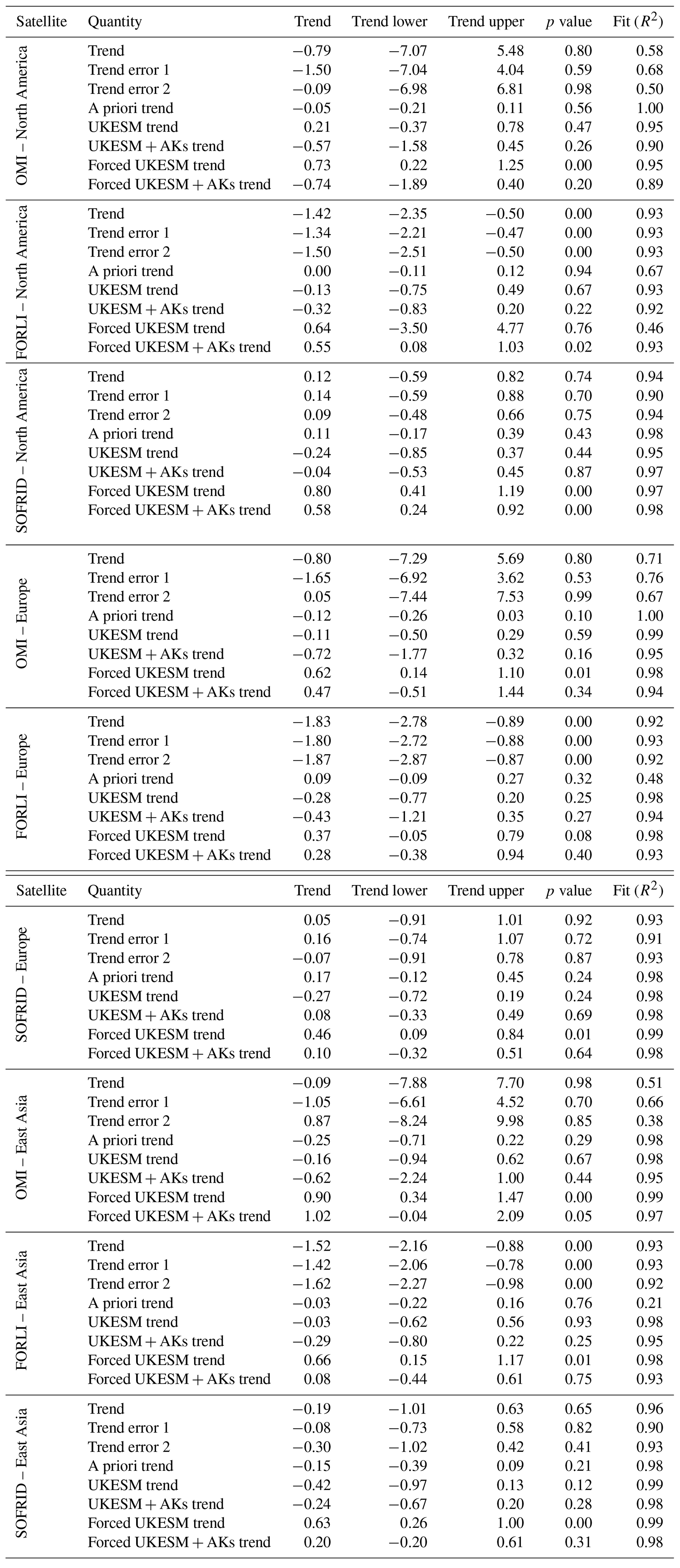
LTCO₃ trends from OMI, IASI-FORLI, IASI-SOFRID, and ozonesondes are derived between 2008 and 2017 (i.e. consistent time record for all instruments) using the linear–seasonal trend model (Eq. 2). For each satellite product, the corresponding UKESM1.0 time series (with and without AKs) are analysed, along with the satellite a priori. For the North America OMI metrics (Fig. 1a, Table 2), there is clear seasonality in the a priori, ranging between approximately 17.0 and 22.0 DU. As this is based on the climatology of McPeters et al. (2007), there is no trend, and there is a very good model fit (i.e. R²=1.0). The key point is that, as a climatology, the a priori will have no trend, but if there are substantial temporal sampling differences between years then an artificial trend could be introduced. OMI LTCO₃ ranges between 20.0 and 27.0 DU, with substantial variability. There is a drop in LTCO₃ to 19.0 DU in 2009 before peaking at 25.0–27.0 DU between 2010 and 2015. Peak LTCO₃ then drops to 22.0–24.0 DU in 2016 and 2017. As a result, the linear–seasonal trend model, which does not account for interannual variations such as this, only has a fit skill of R²=0.59. The corresponding OMI LTCO₃ trend is −0.79[−7.07, 5.48] DU per decade, showing a negligible trend with a large uncertainty range. Here, −0.79 DU per decade is the trend, while [−7.07, 5.48] DU per decade constitute the 95 % confidence interval. The UKESM1.0 LTCO₃ time series ranges between 17.0 and 22.0 DU, with clear seasonality though somewhat less interannual variation than OMI, and the linear–seasonal trend model therefore has a considerably better fit with R²=0.95. The model trend has the opposite sign at 0.21[−0.37, 0.78] DU per decade. Here, the model trend is near-zero, with a relatively large uncertainty range (though not as sizable as OMI). When the AKs are applied to the model, the trend switches sign to −0.57[−1.58, 0.45] DU per decade, and the linear–seasonal trend model fit decreases in skill to R²=0.90. The trend switch in sign, though small, is potentially linked to the application of the AKs, which also increases LTCO₃ by 2.0–3.0 DU in general.

Table 2 LTCO₃ trends (DU per decade) for the satellite trend (trend), the satellite − uncertainty trend (trend error 1), the satellite + uncertainty trend (trend error 2), the satellite a priori trend (a priori trend), the UKESM trend (UKESM trend), the trend of UKESM with AKs applied (UKESM + AKs trend), the forced UKESM trend (forced UKESM trend) and the trend of the forced UKESM with AKs applied (forced UKESM + AKs trend). The “trend lower” and “trend upper” represent the trend 95 % confidence interval based on the trend precision calculated from Eq. (3). R² is the trend fit skill (i.e. correlation squared), and the p value is also shown.

We also investigated the satellite degrees of freedom of signal (DOFS) over the lower troposphere (i.e. surface to 450 hPa), which provides an estimate of the number of independent pieces of information in the LTCO₃. The DOFS are calculated by taking the trace of the AK matrix over the lower-tropospheric levels in the satellite vertical grid. Overall, we found that the products for the three regions had negligible trends in their time series (i.e. within ± 1.0 % yr⁻¹), meaning that the information content of satellite LTCO₃ remained stable with time (see Sect. S3 in the Supplement).

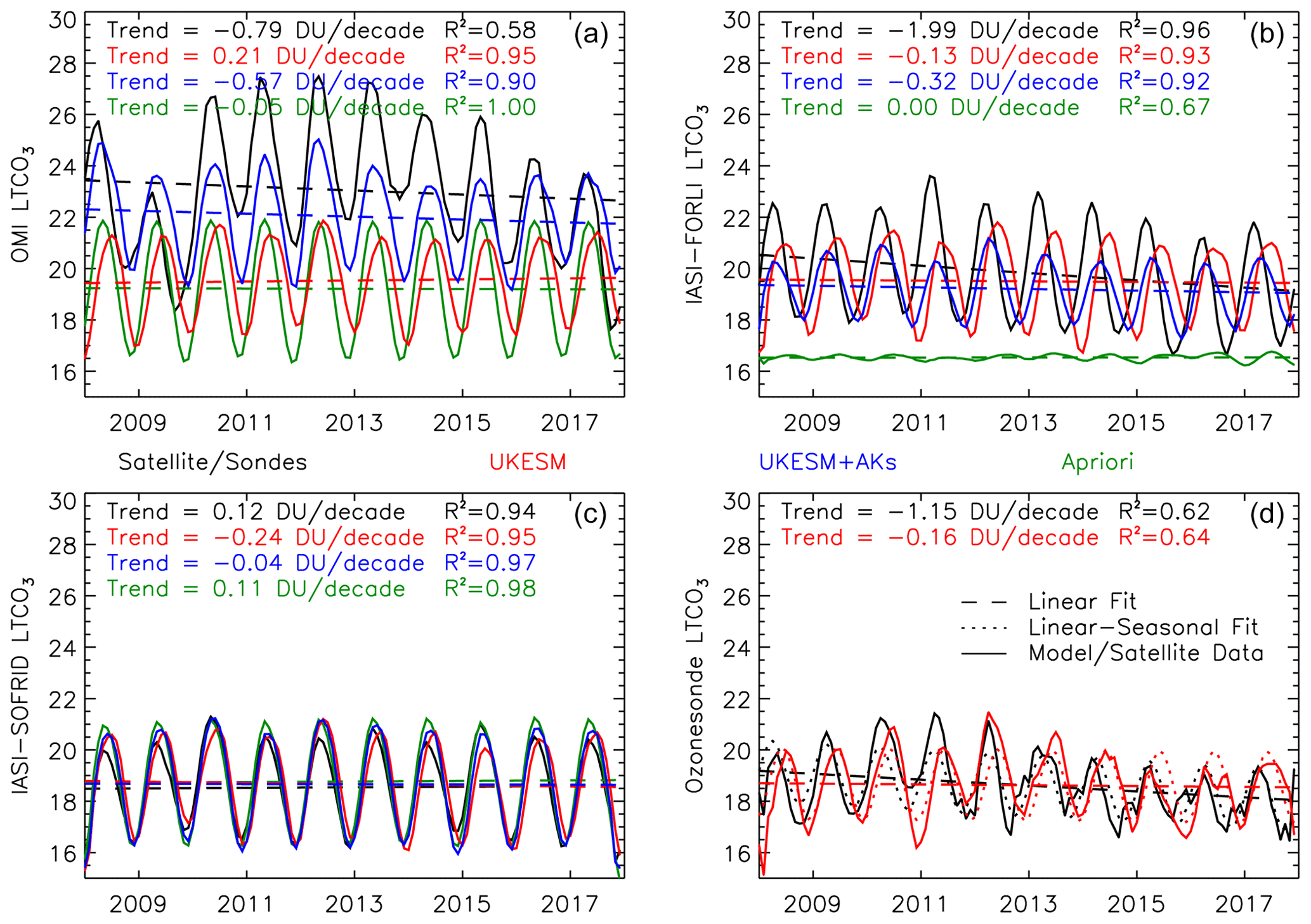
Figure 1 Lower-tropospheric column ozone (LTCO₃, surface to 450 hPa, DU) regional time series for North America, based on the HTAP land mask, from OMI (a), IASI-FORLI (b), IASI-SOFRID (c), and ozonesondes (d), are shown by the black lines in the respective panels. UKESM1.0 simulations without and with satellite averaging kernels (AKs) applied are shown in red and blue lines. Green lines show the satellite a priori. Dashed lines show the LTCO₃ linear trends, which are labelled at the top of each panel. The R²-squared values show the linear–seasonal trend model fit to the corresponding LTCO₃ time series (i.e. correlation squared).

The IASI-FORLI LTCO₃ time series (Fig. 1b) tends to be lower than that of OMI and ranges between 17.0 and 22.0 DU. There is a substantial negative IASI-FORLI trend (−1.42[−2.35, −0.50] DU per decade; Table 2), although, as stated by Boynard et al. (2018) and Wespes et al. (2018), the IASI level-1 data sets input into the FORLI retrieval are not consistent with time; they suffer from a specific discontinuity in September 2010, which degrades the robustness of this trend. While we are aware of the artificial trend in the IASI-FORLI data set, it is still a valuable long-term product, allowing us to quantify multiple factors (e.g. impact of AKs on model tendencies and absolute values and year-to-year spatio-temporal sampling stability – i.e. near-zero trend in the a priori). The a priori has a negligible trend, but there is no clear seasonality in the a priori time series. As a result, the linear–seasonal trend model has a more limited fit skill (i.e. R²=0.67). The impact of the satellite AKs appears to be less for IASI-FORLI as both UKESM1.0 and UKESM1.0 + AKs have time series ranging between approximately 17.0 and 21.0 (though the UKESM1.0 + AKs range is slightly smaller) and linear–seasonal trend model fits of R²=0.93 and R²=0.92, respectively. The corresponding trends are small at −0.13[−0.75, 0.49] DU per decade and −0.32 [−0.82, 0.20] DU per decade, but the introduction of the AKs does move the UKESM1.0 trend slightly towards that of the satellite. Interestingly, while the application of the IASI-FORLI AKs to UKESM marginally pushes the convolved model trend in LTCO₃ towards that of the satellite (which has a substantial negative trend), the IASI-FORLI DOFS have small positive trends (0.37 % yr⁻¹–0.57 % yr⁻¹ – see Sect. S3 in the Supplement). Therefore, there is a minor-scale, yet contrasting, discrepancy in how the vertical sensitivity influences the long-term LTCO₃ trends.

For IASI-SOFRID (Fig. 1c), there is little difference between any of the time series as they all range between 16.0 and 21.0 DU, with corresponding linear–seasonal trend model fits of R²=0.94 to 0.98 and negligible trends. The IASI-SOFRID and a priori trends are 0.12[−0.59, 0.82] DU per decade and 0.11[−0.17, 0.39] DU per decade (Table 2), respectively, with the model showing near-zero trends in both cases. Given the close agreement between the satellite and a priori time series and fit metrics, it is suggestive that IASI-SOFRID TO₃ is more closely confined to the a priori profile than are the other products.

The ozonesondes show a substantial trend of −1.15[−2.0, −0.10] DU per decade, while the model trend sampled as the sondes is −0.16[−1.67, 1.35] DU per decade. The co-located model and ozonesonde linear–seasonal trend model fits are R²=0.62 and 0.64, respectively. The noise and lack of seasonality in the ozonesonde time series are slightly unexpected given the reasonable density of stations across North America, though the spatial coverage and temporal sampling are much less than for the satellite products.

3.1.2 Europe

In Europe, the OMI LTCO₃ values are larger than in North America, ranging between 19.0 and 30.0 DU (Fig. 2a). The same interannual variability exists, peaking between 2010 and 2015, with the minimum in 2009. Hence, the linear–seasonal trend model, which does not represent interannual variation, has moderate skill and R²=0.72. The corresponding trend is −0.80[−7.29, 5.69] DU per decade and so has a similar direction and magnitude to that for North America, though this is not substantial. The a priori ranges between 17.0 and 22.5 DU, with a trend of −0.12[−0.26, 0.03] DU per decade (Table 2). Given the relatively small trend and uncertainty range, unlike for the OMI equivalent, this suggests that there is unlikely to be an artificial trend arising through year-to-year spatio-temporal sampling changes in geographical sampling across the European region. UKESM1.0 LTCO₃ ranges between approximately 19.0 and 22.0 DU, with a good linear–seasonal trend model fit of R²=0.99 and a trend of −0.11[−0.50, 0.29] DU per decade. As for North America, when the OMI AKs are applied, the UKESM LTCO₃ values systematically increase by 2.0–3.0 DU, move further away from the satellite a priori, and more closely follow the variability of OMI (R² decreases slightly to 0.95). The trend tends towards that of OMI at −0.72[−1.77, 0.32] DU per decade.

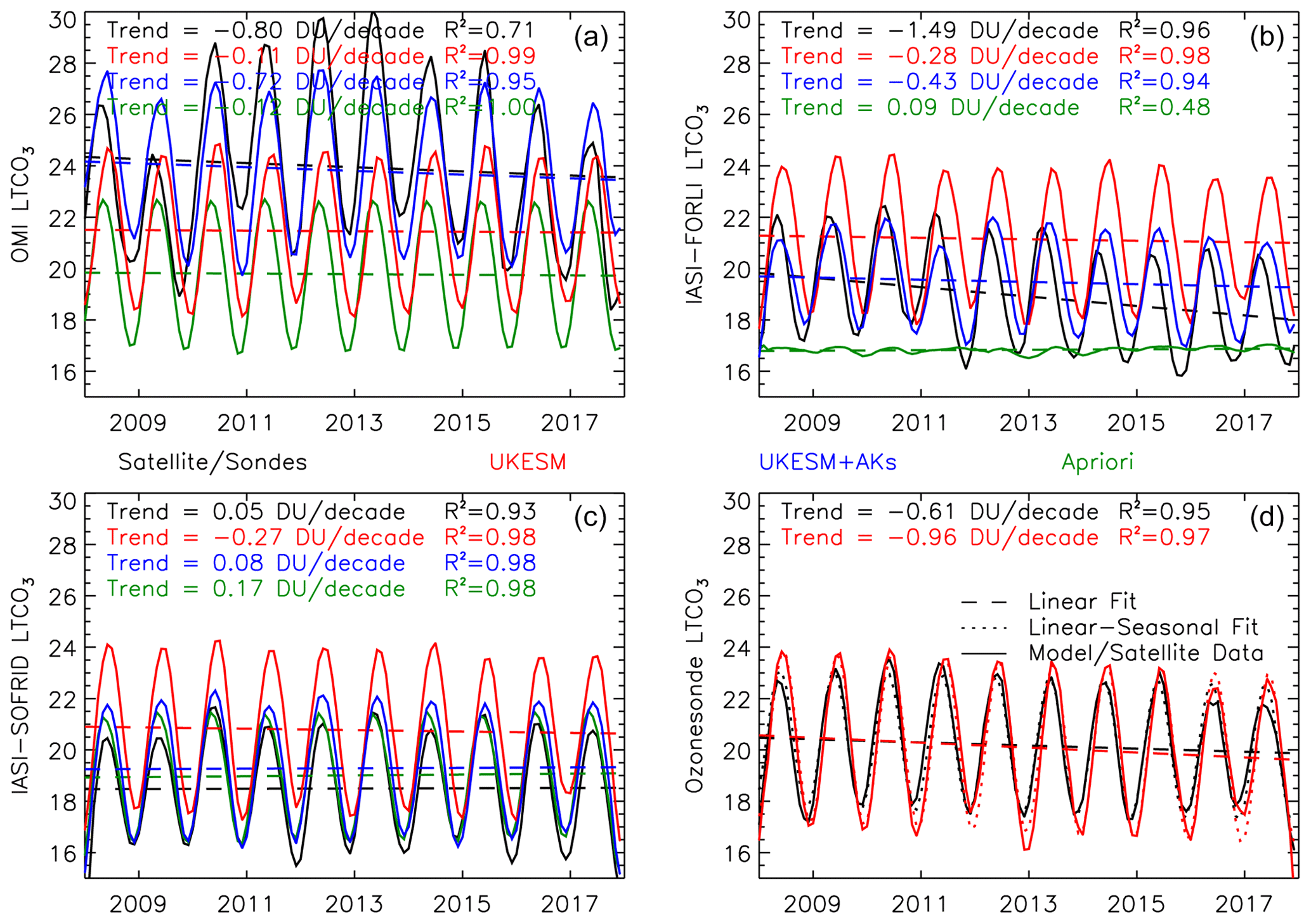
Figure 2 LTCO₃ (DU) regional time series for Europe, based on the HTAP land mask, from OMI (a), IASI-FORLI (b), IASI-SOFRID (c), and ozonesondes (d), are shown by the black lines in the respective panels. UKESM1.0 simulations without and with satellite AKs applied are shown in red and blue lines. Green lines show the satellite a priori. Dashed lines show the LTCO₃ linear trends, which are labelled at the top of each. The R²-squared values show the linear–seasonal trend model fit to the corresponding LTCO₃ time series (i.e. correlation squared).

As in the case of North America, the European IASI-FORLI a priori has no seasonal cycle (and moderate R² of 0.48 in the linear–seasonal trend model fit) with a near-zero trend (0.09[−0.09, 0.27] DU per decade) (Fig. 2b, Table 2). The IASI-FORLI data exhibit a substantial negative trend of −1.83[−2.78, −0.89] DU per decade, again due to step changes in the IASI level-1 processor, with a good linear–seasonal trend model fit of R²=0.92. UKESM1.0 LTCO₃ trends, without and with AKs applied, are −0.28[−0.77, 0.20] DU per decade and −0.43[−1.21, 0.35] DU per decade. Again, though a small change, the application of the AKs introduces a slight perturbation of the model trend compared to IASI-FORLI.

The IASI-SOFRID a priori, ranging between 17.0 and 21.0 DU, has a trend of 0.17[−0.12, 0.45] DU per decade, with a good fit skill of R²=0.98 (Fig. 2c). The IASI-SOFRID and UKESM1.0 metrics, with and without averaging kernels applied, are similar, with LTCO₃ trends of 0.05[−0.91, 1.01] DU per decade, −0.27 [−0.72, 0.19] DU per decade, and 0.08[−0.33, 0.49] DU per decade, respectively, and with R² values between 0.93 and 0.98.

The ozonesonde monthly regional means (Fig. 2d) have a more pronounced time series than for North America, yielding a less noisy time series of LTCO₃. Here, there is clear seasonality ranging between 17.0 and 24.0 DU, with a large R² value of 0.95. The ozonesonde trend is relatively small at −0.6[−1.39, 0.17] DU per decade, while the UKESM1.0 equivalent is more substantial at −0.96[−1.56, 0.35] DU per decade.

3.1.3 East Asia

For East Asia, OMI LTCO₃ again has both a pronounced seasonal cycle and interannual variability (19.0–27.0 DU), which is consistent with the other two regions discussed above (Fig. 3a, Table 2). This yields a moderate skill fit to the linear–seasonal trend model of R²=0.52 and a near-zero trend (−0.09[−7.88, 7.70] DU per decade). The a priori has a trend of −0.25[−0.71, 0.22] DU per decade; thus, year-to-year spatio-temporal sampling changes could be influencing the robustness of OMI retrieved time series in this region. However, both the instrument and a priori trend uncertainties intersect with 0.0. UKESM1.0 LTCO₃ ranges between approximately 16.0 and 22.0 DU, with a good fit of R²=0.98. Like the other regions, the application of the OMI AKs increases the model values systematically by several Dobson units. The UKESM1.0 LTCO₃ trend is −0.16[−0.94, 0.62] DU per decade, which is small, but the AKs increase the trend magnitude to −0.62[−2.24, 1.00] DU per decade, which moves it away from the OMI trend.

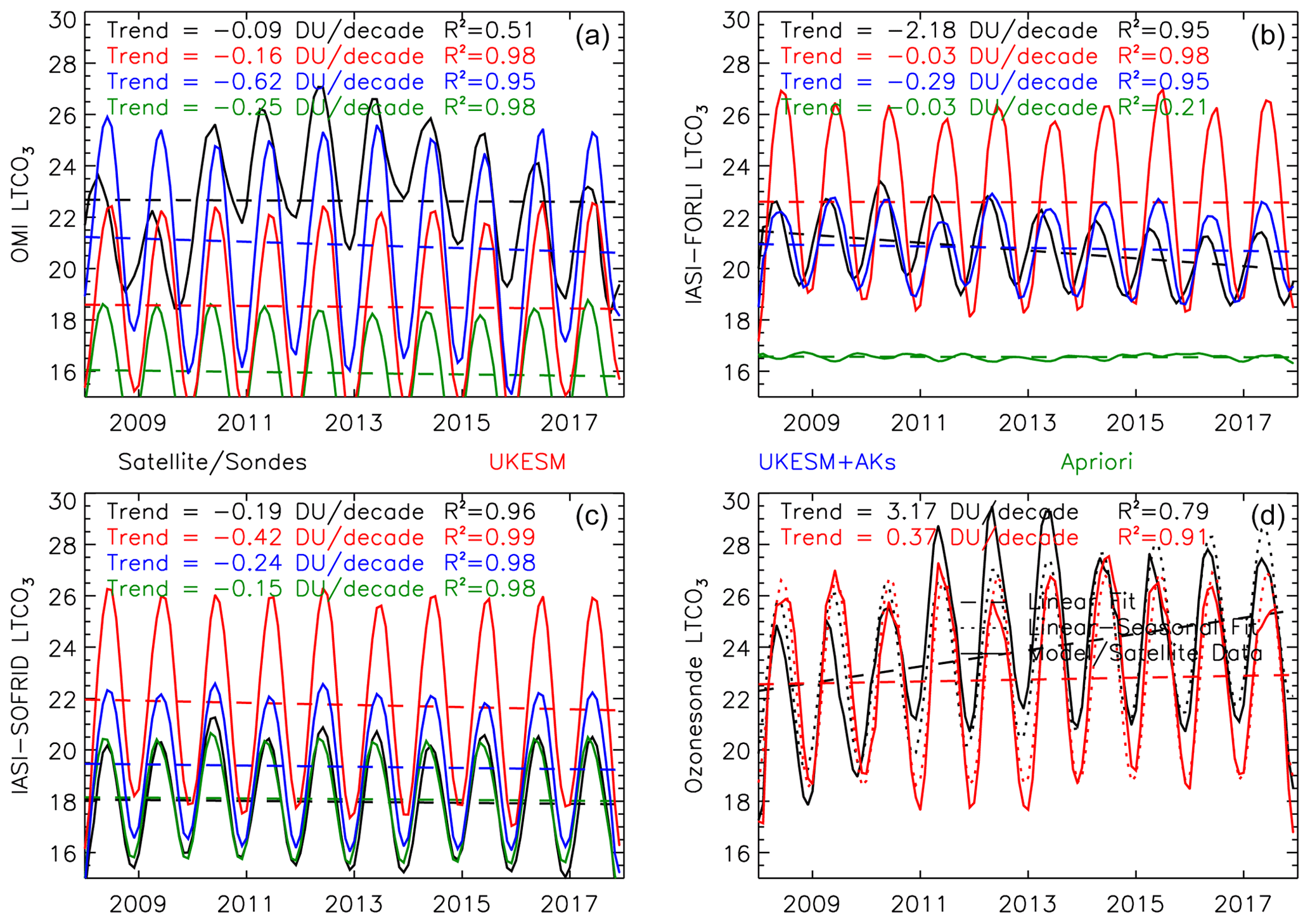
Figure 3 LTCO₃ (DU) regional time series for East Asia, based on the HTAP land mask, from OMI (a), IASI-FORLI (b), IASI-SOFRID (c), and ozonesondes (d), are shown by the black lines in the respective panels. UKESM1.0 simulations without and with satellite AKs applied are shown in red and blue lines. Green lines show the satellite a priori. Dashed lines show the LTCO₃ linear trends, which are labelled at the top of each panel. The R²-squared values show the linear–seasonal trend model fit to the corresponding LTCO₃ time series (i.e. correlation squared).

IASI-FORLI (Fig. 3b, Table 2), like the other two regions, has a substantial negative trend of −1.52[−2.16, −0.88] DU per decade. The a priori again exhibits virtually no seasonal cycle (low fit skill of R²=0.21) and negligible year-to-year spatio-temporal sampling differences yielding a near-zero trend of −0.03[−0.22, 0.16] DU per decade. For UKESM1.0, the East Asian seasonal range is much larger than that of other regions, ranging between 17.0 and 27.0 DU (i.e. seasonal amplitude of approximately ± 5.0 DU). When the AKs are applied, this range shrinks to approximately 19.0 to 23.0 DU, which is more in line with the IASI-FORLI LTCO₃ values. The corresponding model trends are −0.03[−0.62, 0.56] DU per decade and −0.29[−0.80, 0.22] DU per decade; thus, the AKs push the model tendency towards that of the instrument, though the impact is small in absolute terms (large in relative terms).

IASI-SOFRID and its a priori LTCO₃ seasonality are, again, very similar, ranging between 16.0 and 21.0 DU, with very little interannual variability and with linear–seasonal trend model fit skills of R²=0.96 and 0.98 (Fig. 3c, Table 2). The IASI-SOFRID and a priori linear trends are therefore also consistent at −0.19[−1.01, 0.63] DU per decade and −0.15[−0.73, 0.58] DU per decade. The UKESM1.0 seasonal variability is, again, large, between 17.0 and 26.0 DU, and, as in the case of IASI-FORLI, when the instrument AKs are applied to the model, the seasonal range shrinks (i.e. 16.0–22.0 DU) to be much closer to the ranges of the retrieval and its prior. The model trends are −0.42[−0.97, 0.13] DU per decade and −0.24[−0.67, 0.20] DU per decade (with AKs), where there is a minor shift in the model tendency towards that of IASI-SOFRID and its prior.

For the ozonesondes (Fig. 3d), there is a substantial LTCO₃ trend of 3.17[0.16, 6.17] DU per decade, with a fit skill of R²=0.79, which is larger than those for North America and Europe. LTCO₃ increases from 18.0–25.0 in 2008 to 21.0–28.0 in 2011. This remains similar in 2012 and 2013 before dropping by several Dobson units between 2014 and 2017. The UKESM1.0 sampled as the ozonesondes has considerably less interannual variability, with a smaller trend of 0.37[−0.90, 1.64] DU per decade. Therefore, UKESM1.0 and the satellite product trends are generally smaller (in magnitude) than the ozonesonde tendencies. However, it is worth considering that there are only a few sites (e.g. Hong Kong and Taiwan) where ozonesonde data are available in East Asia.

3.2 Influence of satellite averaging kernels on UKESM1.0 LTCO₃

To investigate the impact of applying the satellite averaging kernels to UKESM1.0 – and, thus, to learn something about the influence of vertical sensitivity on retrieved LTCO₃ – three different metrics are considered for the 2008–2017 time-period. These are the absolute LTCO₃ value, the amplitude of the LTCO₃ seasonal cycle, and the linear trend. These metrics are compared for the satellite, the satellite ± the error term, the a priori, UKESM1.0, and UKESM1.0 + AKs for the three regions discussed above.

From Fig. 4, the average OMI LTCO₃ is approximately 22.0, 24.0, and 23.0 DU for North America, Europe, and East Asia, respectively. This represents a substantial deviation from the a priori values of 17.5, 20.0, and 16.0 DU, respectively. However, the average error term for OMI LTCO₃ is sizeable at approximately ± 8.0 to ± 9.0 DU for all regions. The average UKESM1.0 values for each region are approximately 19.5, 21.5, and 19.0 DU, but the application of the AKs increases this by several Dobson units to 22.0, 24.0, and 21.0 DU. In comparison, mean values for both IASI products vary less between the three geographical areas: IASI-FORI (IASI-SOFRID) LTCO₃ values are 20.0 (18.5), 19.0 (18.5), and 22.0 (18.0) DU. The corresponding error ranges, in comparison with OMI, are smaller between 17.0 and 23.0 (16.0 and 21.5), 16.0 and 21.5 (16.0 and 21.0), and 18.0 and 23.5 (14.5 and 21.5) DU for North America, Europe, and East Asia, respectively. With the IASI-FORLI AKs applied to UKESM1.0, LTCO₃ decreases from 19.5–19.25, 21.25–19.5, and 22.75–21.25 DU for the three regions. For IASI-SOFRID, there is a decrease from 21.0–19.5 DU in Europe and a decrease from 22.0–19.5 DU in East Asia, while no change occurs in North America. Overall, OMI has the largest error range, and the application of the AKs to UKESM1.0 systematically increases the model LTCO₃ time series by several Dobson units. The opposite occurs for the IASI products where there is a smaller decrease to UKESM1.0 LTCO₃ of 1.0–2.0 DU. The error ranges are also smaller than that of OMI.

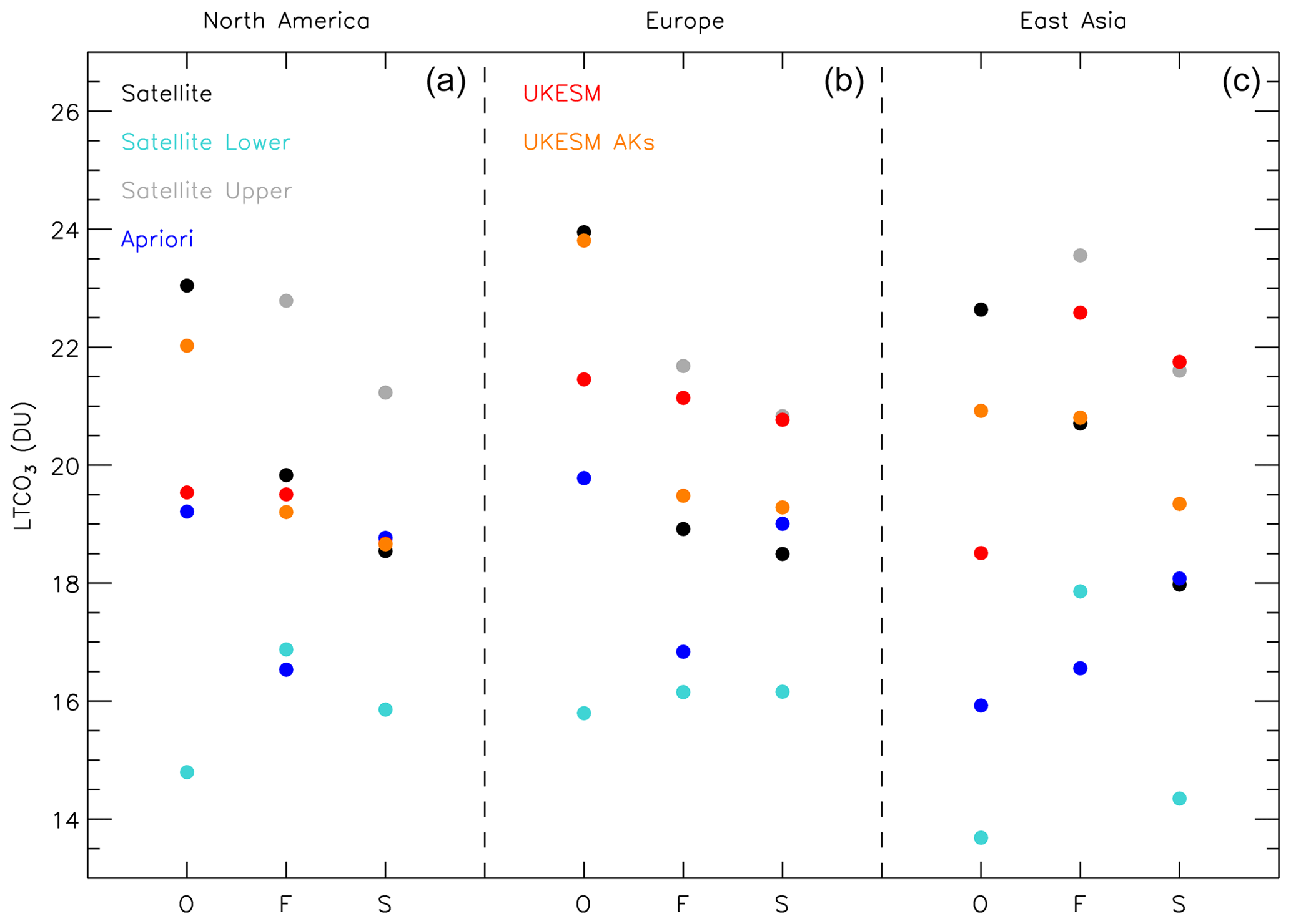
Figure 4 Average LTCO₃ (DU) values across the 2008–2017 time period for the satellite (black), lower satellite (cyan), upper satellite (grey), a priori (blue), UKESM1.0 (red), and UKESM1.0 + AKs (orange). The lower-satellite and upper-satellite values are the average of the satellite ± its error term time series (note: these values do not always fit in the y-axis range). O, F, and S represent OMI, IASI-FORLI, and IASI-SOFRID for North America (a), Europe (b), and East Asia (c).

In terms of the LTCO₃ seasonal amplitude (Fig. 5), OMI (including the error terms) is approximately 2.6 DU (for all), 3.3–3.8, and 2.3–2.6 DU for North America, Europe, and East Asia. The a priori seasonal amplitude ranges from 2.7 to 2.9 DU across the regions. The IASI-FORLI averages (including the error terms) tend to be lower than OMI but have similar seasonal ranges. North America, Europe, and East Asia have amplitudes of 2.3–2.5, 2.3–2.5, and 1.6–1.8 DU, respectively. It is noteworthy that this seasonal cycle occurs despite the IASI-FORLI prior exhibiting virtually no seasonal cycle at all. IASI-SOFRID has a European range of 2.4–2.6 DU and comparable ranges for North America and East Asia at 1.8–2.5 and 2.3–3.0 DU. Therefore, the seasonal amplitude in IASI-SOFRID is more sensitive to the error metric, but as the “error” term is based on the LTCO₃ standard deviation, given the lack of an error term in the product, it is unsurprising that there is more variability in the seasonal amplitude. For the OMI comparisons, the application of the AKs to UKESM1.0 shifts the simulated amplitude slightly upwards from 2.0–2.1, 3.1–3.3, and 4.0–4.4 DU for the respective regions. The IASI-FORLI AK impacts are a decrease from 1.9–1.4, 3.0–2.1, and 4.2–1.9 DU. For IASI-SOFRID, the corresponding impact on UKESM1.0 is 2.2–2.4, 3.3–2.9, and 4.5–3.2 DU. Therefore, the OMI AKs have a minimal impact, increasing the model seasonal amplitude by 0.1–0.3 DU, but the IASI products suppress the simulated amplitude by 1.0–2.0 DU at the most extreme.

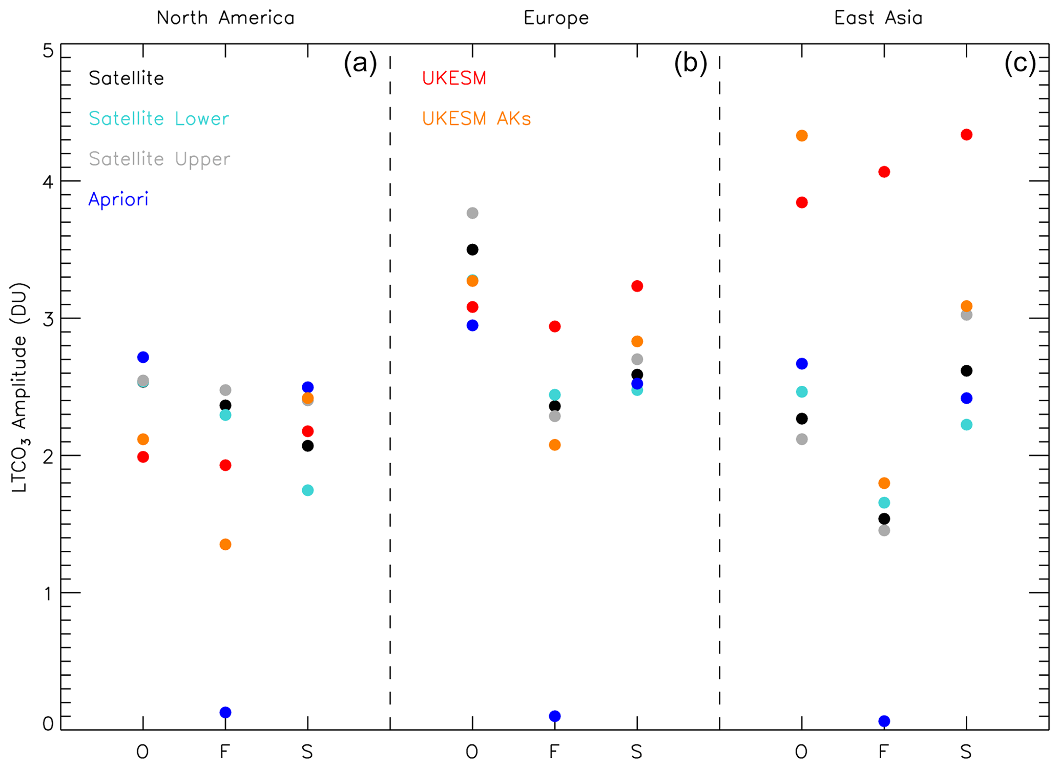
Figure 5 Average LTCO₃ seasonal-cycle amplitude (DU) values across the 2008–2017 time period for the satellite (black), lower satellite (cyan), upper satellite (grey), a priori (blue), UKESM1.0 (red), and UKESM1.0 + AKs (orange). The lower-satellite and upper-satellite values are the average of the satellite ± its error term time series (note: these values do not always fit in the y-axis range). O, F, and S represent OMI, IASI-FORLI, and IASI-SOFRID for North America (a), Europe (b), and East Asia (c).

The impacts of the satellite LCTO₃ error terms on the derived linear trends are shown in Fig. 6. For OMI, the range in trends calculated (i.e. satellite ± error term) is approximately −1.50[−7.04, 4.04] DU per decade to −0.09 [−6.98, 6.81] DU per decade, −1.65[−6.92, 3.62] DU per decade to 0.05[−7.44, 7.53] DU per decade, and −1.05[−6.61, 4.52] DU per decade to 0.87[−8.24, 9.98] DU per decade for North America, Europe, and East Asia, respectively. The IASI-FORLI trends (i.e. satellite ± error term) are substantial, ranging from −1.50[−2.51, −0.50] DU per decade to −1.34[−2.21, −0.47] DU per decade, −1.87[−2.87, −0.87] DU per decade to −1.80[−2.72, −0.88] DU per decade, and −1.62[−2.27, −0.98] DU per decade to −1.42[−2.06, −0.78] DU per decade for the three regions. The corresponding IASI-SOFRID trends were 0.09[−0.48, 0.66] DU per decade to 0.14[−0.59, 0.88] DU per decade, −0.07[−0.91, 0.78] DU per decade to 0.16[−0.74, 1.07] DU per decade, and −0.30[−1.02, 0.42] DU per decade to −0.08[−0.73, 0.58] DU per decade. Therefore, only the IASI-FORLI trends (i.e. satellite ± error term) are substantially different from zero (i.e. p < 0.05). However, that is due in part to discontinuities in the input meteorological data used to generate this version of the product (Boynard et al., 2018).

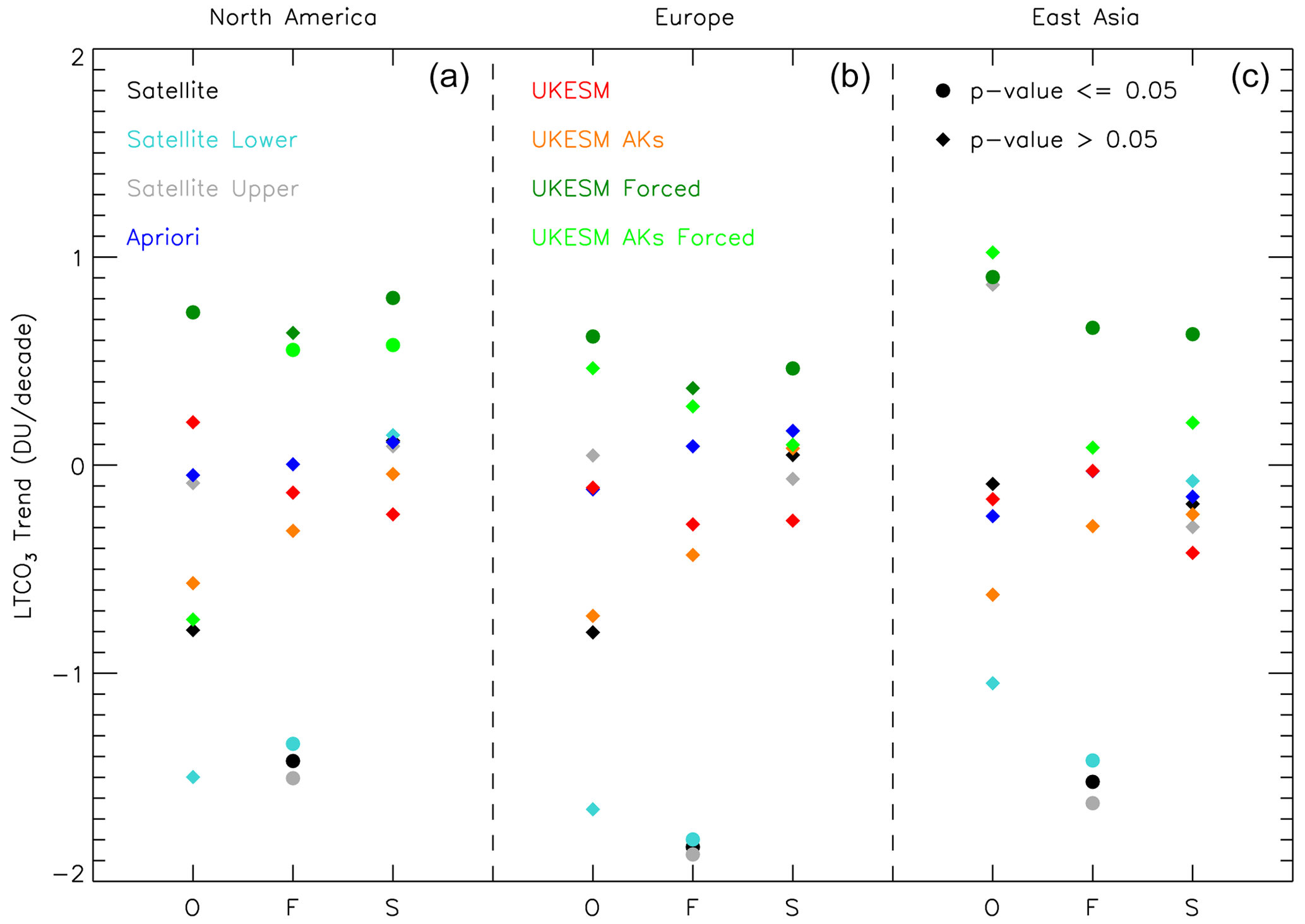
Figure 6 Average LTCO₃ linear trends (DU per decade) across the 2008–2017 time period for the satellite (black), lower satellite (cyan), upper satellite (grey), a priori (blue), UKESM1.0 (red), UKESM1.0 + AKs (orange), forced UKESM1.0 (dark green), and forced UKESM1.0 + AKs (light green). The lower-satellite and upper-satellite values are the average of the satellite ± its error term time series (note: these values do not always fit in the y-axis range). O, F, and S represent OMI, IASI-FORLI, and IASI-SOFRID for North America (a), Europe (b), and East Asia (c). Diamond and circular symbols represent linear trends with p values > 0.05 or p ≤ 0.05, respectively.

The application of the OMI AKs to UKESM1.0 had the largest impacts on the simulated trends, with changes in a negative direction from 0.21[−0.37, 0.78] DU per decade to −0.57[−1.58, 0.45] DU per decade, −0.11[−0.50, 0.29] DU per decade to −0.72[−1.77, 0.32] DU per decade, and −0.16[−0.94, 0.62] DU per decade to −0.62[−2.24, 1.00] DU per decade for the respective regions. IASI-FORLI AKs introduced small decreases from −0.13[−0.75, 0.49] DU per decade to −0.32[−0.82, 0.20] DU per decade, −0.28[−0.77, 0.20] DU per decade to −0.43[−1.21, 0.35] DU per decade, and −0.03[−0.62, 0.56] DU per decade to −0.29[−0.80, 0.22] DU per decade. IASI-SOFRID AKs introduced small increases in the LTCO₃ trend from −0.24[−0.85, 0.37] DU per decade to −0.04[−0.53, 0.45] DU per decade, −0.27[−0.72, 0.19] DU per decade to 0.08[−0.33, 0.49] DU per decade, and −0.42[−0.97, 0.13] DU per decade to −0.24[−0.67, 0.20] DU per decade.

As the absolute model trends are small, it is difficult to determine the impact of the AKs on the simulated trends. In relative terms, it can have impacts of several hundred percent, but the model and model + AK trend ranges (95 % confidence interval) always intersect. Therefore, in an attempt to derive more substantial UKESM1.0 LTCO₃ trends (without and with AKs applied) in order to assess the maximum impact the AKs can have on UKESM LTCO₃ trends, the modelled data were sorted from lowest to highest, and the trend was re-calculated. In North America, this approach forced positive model trends, sub-sampled to OMI, IASI-FORLI, and IASI-SOFRID, of 0.73[0.22, 1.25] DU per decade, 0.64[−3.50, 4.77] DU per decade, and 0.80 (0.41, 1.19) DU per decade. When the AKs were applied, it yielded trends of −0.74[−1.89, 0.40] DU per decade, 0.55[0.08, 1.03] DU per decade, and 0.58[0.24, 0.92] DU per decade. In Europe, this forced positive model trends of 0.62[0.14, 1.10] DU per decade, 0.37[−0.05, 0.79] DU per decade, and 0.46[0.09, 0.84] DU per decade. With the AKs applied, the trends become 0.47[−0.51, 1.44] DU per decade, 0.28[−0.38, 0.94] DU per decade, and 0.10[−0.32, 0.51] DU per decade. Finally, in East Asia, the forced model trends are 0.90[0.34, 1.47] DU per decade, 0.66[0.15, 1.17] DU per decade, and 0.63[0.26, 1.00] DU per decade. The application of the AKs introduced model trends of 1.02[−0.04, 2.09] DU per decade, 0.08[−0.44, 0.61] DU per decade, and 0.20[−0.20, 0.61] DU per decade.

Even with forced trends in the UKESM1.0 regional time series, the trends are relatively small (i.e. typically less than 1.0 DU per decade in magnitude). Therefore, the application of the AKs to the forced UKESM LTCO₃ time series still yields small-scale changes in tendencies, and there is an overlap in the two model trend uncertainty ranges (i.e. 95 % confidence levels). However, in relative terms, the trend changes are larger (e.g. > 100 % in multiple cases), and there is often a shift in the modelled LTCO₃ trend uncertainty range so that it is either intersecting or no longer intersecting with zero (i.e. a shift in the p-value regime from < 0.05 to > 0.05). Therefore, in modelled and satellite data sets with more substantial trends, the impacts of the AKs, and thus of the satellite vertical sensitivity, on LTCO₃ trends would be much greater and could potentially help pinpoint sources of differences between satellite products in terms of their TO₃ temporal evolution.

3.3 Diurnal variability in regional LTCO₃ and temporal evolution

As TO₃ varies diurnally due to meteorological and photochemical processes (e.g. Gaudel et., 2018), the different satellite overpass times (i.e. Aura and Metop-A daytime overpasses are around 13:30 and 09:30 local time, respectively) will likely influence the spatial distributions of TO₃ which OMI and IASI will retrieve. In principle, this could therefore explain some differences between the two sensors and their long-term LTCO₃ trends. Here, the model is a useful tool to help investigate this, and we used the 6-hourly output to derive the UKESM simulated LTCO₃ spatial distributions at the Aura (13:30 LT) and Metop-A (09:30 LT) daytime overpasses. These model fields were then used to calculate regional time series for North America, Europe, and East Asia. For each region and month, between 2008 and 2017, we calculated the regional average absolute difference (i.e. from the selection of model grid cells which fell within the HTAP-2 mask for a specific month) and the standard deviation of the absolute differences between the overpass times. Here, across all months and regions, we found the peak average absolute difference (13:30–09:30 LT) and the standard deviation to be small at 2.03 % and 2.56 %, respectively. For the long-term trends, across all regions and overpass times, all of the UKESM trends were smaller than ± 0.5 DU per decade. Therefore, the model LTCO₃ regional trends are negligibly different between overpass times. This might not be surprising given the negligible model trends in the satellite spatio-temporal trend comparisons (see Sect. 3.1), but the actual absolute differences (average and range) in simulated LTCO₃ are also small, supporting the argument that, on the regional scale, the daytime diurnal-cycle differences between satellite overpass times have a limited influence on the reported satellite trend discrepancies (e.g. in Gaudel et al., 2018).

4 Discussion

This investigation of satellite LTCO₃ focussed on 2008–2017, representing a decade of overlap of the OMI and IASI records. The analysis focussed on North America, Europe, and East Asia as these regions are subject to large emissions of and temporal changes in O₃ precursor gases. LTCO₃ is typically spatially homogeneous, with shallow gradients between background and source-induced O₃ concentrations. Secondly, individual retrievals of LTCO₃ are often associated with large uncertainties (e.g. random and systematic uncertainties). There are multiple contributory factors concerning both instrumental attributes (notably, spectroradiometric noise and calibration accuracy) and variability in geophysical variables which influence radiative transfer and vertical sensitivity (e.g. stratospheric ozone, cloud and aerosol, water vapour, surface spectral reflectivity and/or emissivity, and pressure and temperature profiles) and which can result in LTCO₃ time series with substantial variability and/or noise when derived at a high spatial resolution (e.g. when deriving time series from data gridded at 0.5° or 1.0°). Therefore, we undertake our analysis at the regional (e.g. continental) scale, where more satellite retrievals are included in time series monthly means, yielding a reduction in the random-error component of the sample.

Ideally, this analysis would have utilized several more records (e.g. several UV–Vis and IR products) to quantify long-term trends in LTCO₃ and to investigate the potential reasons for any discrepancies, as shown by Gaudel et al. (2018) for TCO₃. While RAL Space and other providers have generated UV–Vis profile O₃ products for more instruments, e.g. the Global Ozone Monitoring Experiment 1 and 2 (GOME-1 and GOME-2) and the SCanning Imaging Absorption spectroMeter for Atmospheric CHartographY (SCIAMACHY), the GOME-1 and SCIAMACHY records do not overlap with the IASI and OMI records either at all or for a sufficient time period. Secondly, step changes in the GOME-2A level-1 processing scheme used to produce the available LTCO₃ level-2 version mean it is not sufficiently homogeneous (see Pope et al., 2023). For the IR instruments, other potential sensors include the Tropospheric Emissions Spectrometer (TES; Richards et al., 2008) and the RAL Space IASI Extended Infrared Microwave Sounding (IMS; Pimlott et al., 2022) scheme applied to IASI. Unfortunately, the TES record only covers 2005–2013, with decreasing spatial coverage with time, and, at the time of this work, the IASI-IMS product had only been processed on a sub-sampled basis of 1 in 10 d.

In this work, we some find discrepancies in the observed long-term tendencies from the utilized LTCO₃ products in these northern-hemispheric regions. The OMI product is subject to large-scale interannual variability over the 2008–2017 decade, in comparison with which the underlying linear trends are small in absolute terms, with large confidence ranges (i.e. 95 % confidence intervals) intersecting with zero. However, the OMI LTCO₃ product has been shown to be stable over this period relative to ozonesondes by Pope at el. (2023). IASI-FORLI has substantial negative LTCO₃ tendencies, but this is driven by a specific discontinuity in 2010 due to an inhomogeneity in EUMETSAT (water vapour, temperature) data used in IASI-FORLI level-2 processing (Boynard et al., 2018; Wespes et al., 2018). This inhomogeneity induces an artificial drift that explains the substantial negative LTCO₃ trends reported here and in Gaudel et al. (2018). The IASI-SOFRID LTCO₃ and the a priori are very similar, with little interannual variability, which suggests that the IASI-SOFRID O₃ retrieval in this height range is more constrained by the a priori (i.e. less TO₃ sensitivity than the other products – see Sect. S3 in the Supplement). Importantly, analysis of the three products' a priori LTCO₃ records show negligible trends, meaning that year-to-year spatio-temporal sampling differences (i.e. the number of retrievals used in the spatio-monthly regional averages) are not skewing long-term satellite trends. In summary: any underlying linear trend in LTCO₃ occurring during the decade 2008–2017 was masked by interannual variability in the OMI retrieval and by constraint to the a priori in the IASI-SOFRID retrieval; although substantial for IASI-FORLI retrieval, this is due to changing meteorological inputs to the data processing (Boynard et al., 2018; Wespes et al., 2018).

For UKESM1.0, the model exhibits negligible long-term temporal variability in LTCO₃ for all regions and for all the instruments' samplings. Modelled LTCO₃ trends never exceeded 1.0 DU per decade in magnitude and were all deemed to be insignificant due to large associated p values using the linear–seasonal trend model detailed in Sect. 2.3 and Eqs. (2) and (3). The ozonesondes for each region were included to ground-truth the model and satellite trends. The North American sites' LTCO₃ time series were relatively noisy and exhibited considerable interannual variability in their seasonal cycles. The comparatively low level of interannual variability in the European UKESM1.0 record of LTCO₃ was in good agreement with the ozonesondes and so was its low trend, providing confidence in the model over that region. For East Asia, the interannual variability differed substantially between UKESM1.0 and ozonesondes, and the reported ozonesonde trend was significantly much larger than for UKESM1.0. Therefore, when considering UKESM1.0 and the ozonesondes, no consistent LTCO₃ trends can be determined for any of the regions. Overall, taking all data sets into account, LTO₃ appears to have neither increased nor decreased markedly over these three regions between the beginning and end of the study decade (i.e. 2008–2017).

One key aspect of this work was to exploit UKESM1.0 to determine the importance of vertical sensitivity for retrieved LTO₃ and how this influences the reported long-term tendency. In terms of the absolute model trends (with and without the satellite AKs), the impact on LTCO₃ was small, typically with near-zero tendencies and large uncertainty ranges (i.e. the 95 % confidence interval). In relative terms, the changes in model trend values were more substantial on the order of 100 %. To explore this further, the UKESM1.0 LTCO₃ time series (with and without the satellite AKs) were sorted from lowest to highest (based on annual averages) to impose the most substantial trend in the model data. When the trends were re-calculated, the largest model LTCO₃ trends ranged between 0.37 and 0.90 DU per decade. When the AKs were applied, the LTCO₃ trends ranged from −0.74 to 1.02 DU per decade. Again, in relative terms, this represents a large impact of the AKs on simulated LTO₃ tendencies, but in absolute terms, these are small changes. However, it should be noted that many of the 95% confidence intervals shifted between statistical regimes (i.e. a p value ≤ 0.05 vs. a p value > 0.05) once the AKs were applied to the model (i.e. the confidence interval initially did not intersect with zero but then did, or the interval did intersect with zero before shifting to a non-zero range).

Gaudel et al. (2018) suggested two potential reasons for the TCO₃ trend discrepancies in their study:

• time-varying instrument biases or drift

• the impact of satellite vertical sensitivity.

A further two important reasons are as follows:

• Changes over time in latitude–longitude domains sampled by satellite sensors (e.g. GOME-1 has substantial issues after 2003)

• the time period used for the trend analysis.

As stated by Boynard et al. (2018) and Wespes et al. (2018), the IASI-FORLI-v20151001 product has an artificial negative drift with time, explained by a discontinuity found in the level-2 meteorological inputs taken from EUMETSAT. However, in the near-future, a new consistent IASI-FORLI ozone climate data record will be available using homogeneous level-1 and level-2 EUMETSAT meteorological data. The analysis of OMI LTCO₃ by Pope et al. (2023) showed OMI LTCO₃ to be temporally stable against ozonesondes. A similar analysis (not shown here) indicates that IASI-SOFRID LTCO₃ is also temporally stable, with near-zero drift in bias. For the satellite vertical sensitivity, some of our results were unexpected. While the application of the AKs to UKESM1.0 can substantially shift the simulated absolute LTO₃ values and squash or stretch the seasonal amplitude, the impacts on the simulation LTCO₃ tendencies are small in absolute terms. In relative terms, the impacts can be large (e.g. 100 % change in trend rate). However, as the UKESM1.0 simulated LTCO₃ trends are generally near zero, it is difficult to confidently say either way if the vertical sensitivity, when retrieving LTCO₃, is important for influencing long-term tendencies, even when a more substantial trend is forced upon UKESM1.0. Future work on this would probably need to look at artificial model data which already contain substantial TO₃ trends (e.g. 5.0 or 10.0 DU per decade). This will obviously not match reality but would provide some further quantification on how important vertical sensitivity is in relation to different instruments or sounders in LTO₃ trend determination.

As for year-to-year spatio-temporal sampling, our results suggest negligible trends for the product LTCO₃ a priori time series; thus, monthly sampling biases are unlikely to introduce artificial trends as the a priori data sets are trendless. Finally, the time period over which the trend analysis is undertaken is critically important. Gaudel et al. (2018), using the available data at the time, focussed on 2005–2015 and 2016 and 2008–2015 and 2016 for the OMI and IASI products they used. For the IASI products, using a slightly extended time period, the trends show similar tendencies. However, for OMI, 2016 and 2017 represent years of lower TO₃. As a result, this dampens the strong significant positive trends in TCO₃ reported by Gaudel et al. (2018). It is notable that the substantial positive increase in tropical LTO₃ between 1995 and 2017 reported by Pope et al. (2023) from a series of UV–Vis sounders, including the same OMI global data set that is used here, further suggests that the selection of the time period and geographical region is crucial with regard to the role of interannual variability in linear trend detection.

5 Conclusions

Gaudel et al. (2018) undertook a multi-satellite analysis of long-term trends in tropospheric column ozone (TCO₃). They found large-scale differences between these products with no clear consensus on the signs or drivers of these TCO₃ trends. To avoid complications with regard to tropopause definition and to reduce the influence of stratospheric ozone on retrieved values, this study has undertaken a detailed follow-up assessment of decadal trends in LTCO₃ (surface–450 hPa layer) rather than TCO₃, exploiting ozonesonde records and model simulations and accounting carefully for satellite O₃ metrics (e.g. averaging kernels (AKs), a priori information, and satellite uncertainties). We have focussed on LTCO₃ data sets from the Ozone Monitoring Instrument (OMI) produced by the RAL Space scheme and from the Infrared Atmospheric Sounding Interferometer (IASI) produced by the IASI-FORLI and IASI-SOFRID schemes, for which there were consistent records from the period 2008–2017.

The evaluation of satellite LTO₃ from these three products over the North American, European, and East Asian regions resulted in linear trends which varied over a small range close to zero and with confidence intervals intersecting with zero. This was consistent with simulations from the UK Earth System Model (UKESM1.0). There were no large-scale trends in the a priori information; thus, changes in satellite year-to-year spatio-temporal sampling have not been driving inconsistencies between products. When convolving UKESM1.0 with the satellite AKs (i.e. to assess the impact of the satellite vertical sensitivity), it did change the size of the model trend and, in some instances, the direction of the trend, but as the simulated LTO₃ trends were small and insignificant, they had limited influence. Overall, our results show that changes in LTO₃ during the decade 2008–2017 in North America, Europe, and East Asia were dominated by variability in processes which control LTO₃ on shorter timescales.

In the near-future, the new European polar-orbiting mission Metop Second Generation will include IASI Next Generation and Sentinel-5 UV–VIS sounders to provide height-resolved ozone products to extend current missions through to the mid-2040s. This will be supplemented by the new USA Near Earth Orbit Network (NEON) series as a replacement for the Joint Polar Satellite System (JPSS). The Geostationary Environment Monitoring Spectrometer (GEMS) and Tropospheric Emissions: Monitoring of Pollution (TEMPO) have also recently been launched, and there will be new geostationary platforms: the Infrared Sounder (IRS) and Sentinel-4 UV–VIS sounder on Europe's Meteosat Third Generation (MTG-S), again through to the mid-2040s, and the USA Geostationary Extended Observations (GeoXO) series. Overall, these platforms will provide large volumes of data (e.g. diurnal observations) on tropospheric ozone over a long timescale for future regional trend analyses.