the Creative Commons Attribution 4.0 License.
the Creative Commons Attribution 4.0 License.
 | 15 Aug 2024
Quantifying the diurnal variation in atmospheric NO2 from Geostationary Environment Monitoring Spectrometer (GEMS) observations
Sara Martínez-Alonso
Duseong S. Jo
Ivan Ortega
Louisa K. Emmons
John J. Orlando
Helen M. Worden
Jhoon Kim
Hanlim Lee
Junsung Park
Hyunkee Hong
The Geostationary Environment Monitoring Spectrometer (GEMS) over Asia is the first geostationary Earth orbit instrument in the virtual constellation of sensors for atmospheric chemistry and composition air quality research and applications. For the first time, the hourly observations enable studies of diurnal variation in several important trace gas and aerosol pollutants including nitrogen dioxide (NO2), which is the focus of this work. NO2 is a regulated pollutant and an indicator of anthropogenic emissions in addition to being involved in tropospheric ozone chemistry and particulate matter formation. We present new quantitative measures of NO2 tropospheric column diurnal variation which can be greater than 50 % of the column amount, especially in polluted environments. The NO2 distribution is seen to change hourly and can be quite different from what would be seen by a once-a-day low-Earth-orbit satellite observation. We use GEMS data in combination with TROPOspheric Monitoring Instrument (TROPOMI) satellite and Pandora ground-based remote sensing measurements and Multi-Scale Infrastructure for Chemistry and Aerosols (Version 0, MUSICAv0) 3D chemical transport model analysis to examine the NO2 diurnal variation in January and June 2023 over Northeast Asia and Seoul, South Korea, study regions to distinguish the different emissions, chemistry, and meteorological processes that drive the variation. Understanding the relative importance of these processes will be key to including pollutant diurnal variation in models aimed at determining true pollutant exposure levels for air quality studies. The work presented here also provides a path for investigating similar NO2 diurnal cycles in the new Earth Venture Instrument-1 Tropospheric Emissions: Monitoring Pollution (TEMPO) data over North America, and later over Europe with Sentinel-4.
- Article
(13561 KB) - Full-text XML
- BibTeX
- EndNote


Predicting atmospheric air quality (AQ) requires understanding the processes that emit air pollutants, how these are transported in the atmosphere, the chemical and physical transformations that take place, and the potential impact on health and the environment. Satellite observations provide valuable information on these processes; however, until recently, measurements from an individual platform were limited to twice daily at best when relying on observations from low Earth orbit (LEO). This is now changing with daylight hourly observations of atmospheric trace gases and aerosols from the new geostationary Earth orbit (GEO) satellite sensors. The South Korean GEO-KOMPSAT-2/GEMS (Geostationary Korea Multi-Purpose Satellite-2/Geostationary Environment Monitoring Spectrometer) instrument (Kim et al., 2020) has been operational over Asia since February 2020, NASA's EVI-1 TEMPO (Earth Venture Instrument-1 Tropospheric Emissions: Monitoring Pollution) instrument (Zoogman et al., 2017) was launched in April 2023 to monitor North America, and Europe will be covered by ESA/EUMETSAT Sentinel-4 (Bazalgette Courrèges-Lacoste et al., 2017) in 2025. Common objectives for these missions will provide column products for ozone (O3), nitrogen dioxide (NO2), sulfur dioxide (SO2), formaldehyde (HCHO), and aerosol optical depth, among others, several times per day at 5–10 km px−1 spatial scales. Together with LEO sensors such as JPSS/CrIS (Joint Polar Satellite System/Cross-track Infrared Sounder) (Han et al., 2013), MetOp/IASI (Infrared Atmospheric Sounding Interferometer) (Clerbaux et al., 2009), and Sentinel-5P/TROPOMI (TROPOspheric Monitoring Instrument) (Veefkind et al., 2012), the new GEO missions will form an atmospheric composition satellite virtual constellation with nearly continuous Northern Hemisphere coverage and unprecedented capability to meet the needs of AQ research and applications (CEOS, 2019).
The hourly measurement time resolution is the novel perspective provided by the new GEO platforms and enables the following: (1) investigations of the diurnal processes determining atmospheric composition; (2) improvements in retrieval sensitivity gained with possible longer measurement acquisition dwell times; (3) high observation data density; and (4) the increased probability of obtaining at least some daily cloud-free observations at any given location (e.g., Fishman et al., 2012; Zoogman et al., 2017; Kim et al., 2020). An important role for the GEO sensors will be in detailing how the new hourly information improves our understanding of diurnal changes that take place with pollutant emissions and subsequent chemistry and transport and how this leads to diurnal changes in AQ. In urban and polluted regions, where these diurnal changes are large, this will likely lead to revised estimates for emissions, population exposure, and associated health and environmental risks compared with those previously based on LEO measurements. This work investigates the processes that drive the diurnal variation in NO2 over Northeast Asia, particularly over Seoul, South Korea, using GEMS data in combination with other satellite and ground-based remote sensing measurements and 3D atmospheric chemical transport model (CTM) analysis.
Of the trace gas products that are routinely retrieved from satellite sensor shortwave spectral measurements, NO2 is one of the most reliable due to the relatively strong signal. It plays a central role in atmospheric chemistry and tropospheric O3 and aerosol formation and is photochemically linked with nitrogen oxide (NO) as reactive nitrogen () (Brasseur et al., 1999). NOx emissions occur primarily as NO and have anthropogenic sources associated with high-temperature combustion processes in the power, industry, and transport sectors (e.g., Goldberg et al., 2021; de Foy and Schauer, 2022). Natural sources include lightning, biomass burning, and soil emissions, amongst others (e.g., Griffin et al., 2021; Huber et al., 2020). The NO2 minutes-to-hours daytime lifetime in the planetary boundary layer (PBL) also means that it does not become evenly mixed in the atmosphere, and polluted regions, especially urban areas, often show satellite-derived NO2 column enhancements of many times the background level. These products are, therefore, particularly useful for understanding NOx and other emissions, their subsequent chemical and physical transformations, and attributing pollution trends over time due to emission regulations and other factors such as the COVID pandemic lockdowns and economic downturns (e.g., Duncan et al., 2013; Levelt et al., 2022; de Ruyter de Wildt et al., 2012). This has resulted in a wealth of peer-reviewed literature based on LEO satellite observations detailing pollutant research and AQ applications and management (e.g., Curier et al., 2014; Duncan et al., 2016; Liu et al., 2017). The partitioning of NOx between NO and NO2 is in a photochemical steady state that establishes on a timescale of minutes during daylight hours. Details are given in Brasseur et al. (1999), and the NOx ratio can be represented as follows:
where the square brackets denote concentration (), k is a bimolecular rate coefficient (), j is the photolysis rate (s−1), HO2 is the hydroperoxy radical, and RO2 represents all organic peroxy radicals. The main loss of NOx is through oxidation to the nitrogen reservoirs nitric acid (HNO3) and peroxyacetyl nitrate (PAN). The chemical diurnal cycle is discussed further in Sect. 5.3 based on the GEMS NO2 data and modeling.
Following this introduction (Sect. 1), Sect. 2 describes the remote sensing measurements and the model tools that are used in this work. Section 3 presents the NO2 diurnal variation observed by GEMS at different spatial scales for our January and June 2023 study months, and this is compared with ground-based remote sensing measurements over Seoul in Sect. 4. Model analysis and discussion in Sect. 5 considers the various processes (emissions, chemistry, and meteorology) that drive the NO2 diurnal variation. Conclusions are presented in Sect. 6.
2.1 GEMS
South Korea's GEMS is the first satellite instrument in the GEO constellation and is monitoring AQ over Asia. GEMS was launched in February 2020 by Arianespace from the French Guiana Space Center. Like the TEMPO instrument, GEMS was built by Ball Aerospace & Technologies Corp. GEMS retrievals of O3, NO2, SO2, HCHO, glyoxal (CHOCHO), and aerosols are derived from ultraviolet–visible (UV–vis) measurements (Kim et al., 2020), and the cloud fraction necessary for data filtering is also available for each observation (Choi et al., 2020; Kim et al., 2024). Each day, the field of regard (FOR) shifts westward with the Sun; this provides measurements over India at the end of the day at the expense of losing coverage over Japan when the solar zenith angles become too large. Total column (TotC), stratospheric column (StrC), and (for some products) tropospheric column (TrC) values are retrieved in up to 10 hourly observations during daytime according to the season with a spatial resolution at Seoul of near 7 km × 7.7 km for gases and cloud, whereas this resolution is 3.5 km × 7.7 km for aerosol and surface reflectivity.
The main retrieval challenges for NO2 (e.g., Palmer et al., 2001; Bucsela et al., 2013; Lorente et al., 2017; Geddes et al., 2018; Zara et al., 2018; van Geffen et al., 2020) are (1) the conversion of the observed NO2 slant column density to an inferred vertical column density using an air mass factor (AMF) and (2) the separation of the StrC and TrC. These steps can both lead to significant uncertainties and biases as is well-documented in studies comparing the varying results from different NO2 retrieval algorithms using the same OMI (Ozone Monitoring Instrument; Levelt et al., 2018) satellite measurements (Zara et al., 2018). The AMF is primarily a geometric conversion based on the observation angles, but this must also consider other factors including cloud and aerosol information, terrain reflectivity, and vertical gas profile (Lorente et al., 2017). A CTM is used in this AMF calculation and also in the separation of the StrC and TrC (Lee et al., 2020; Geddes et al., 2018). The NO2 a priori profiles in this GEMS data version are provided by the GEOS-Chem model (Bey et al., 2001). Although beyond the scope of this paper, retrieval sensitivity studies and product validation for the new GEO composition measurements will be important to minimize any aliasing of diurnal variation in the retrieval input parameters onto the diurnal variation in the retrieved products themselves (e.g., Yang et al., 2023a; Kim et al., 2023; Szykman and Liu, 2023). This includes, for example, parameters that impact the AMF, a priori assumptions that change by location and time; angular dependences of surface and cloud reflectivities; vertical profiles of trace gases and aerosols; meteorology; and PBL evolution.
This work uses the publicly available Version 2 (V2.0) NO2 Level-2 data obtainable from the Korean National Institute of Environmental Research (NIER) (NIER, 2024). An example of the coverage is shown in Fig. 1. The data quality flags used are those recommended by the algorithm development team (Lee et al., 2022). These are as follows: FinalAlgorithmFlags ≤1; CloudFraction <0.3; and SolarZenithAngle and ViewingZenithAngle ≤70°. The nominal GEMS pre-launch accuracy for the NO2 TrC is 1×10¹⁵ () (Kim et al., 2020). The Level-2 data contain an error term for the NO2 spectral fit, but this does not account for the AMF calculation error and the conversion to vertical column. Analysis for TROPOMI (van Geffen et al., 2022) identified the latter as the main source of product error (around ±25 % over polluted regions). Comparison of the GEMS L2 NO2 with other measurements is further discussed in Sect. 4. Updates and enhancements to the GEMS retrieval algorithms are ongoing and will result in new data versions being released periodically.
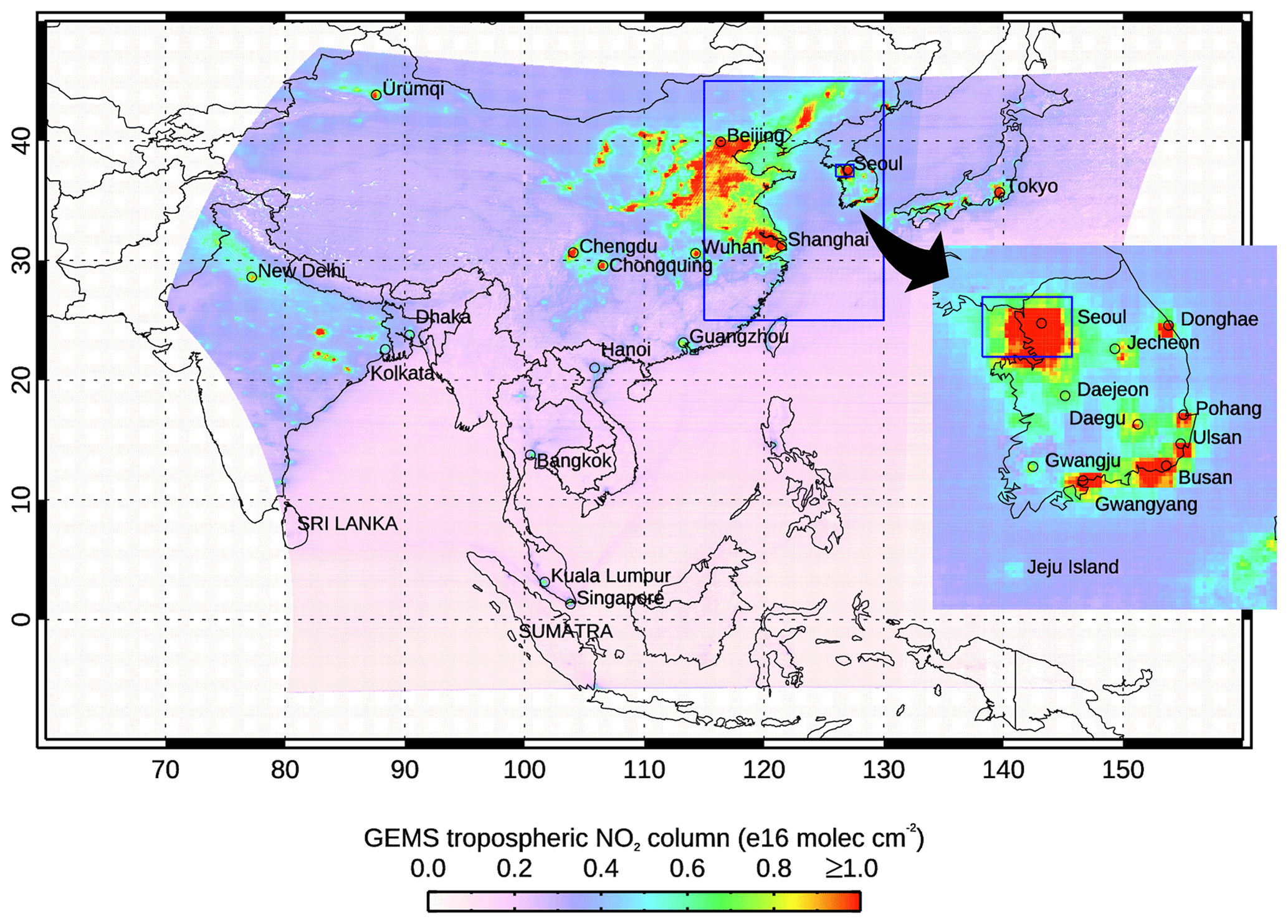
Figure 1Averaged GEMS NO2 TrC for June 2023 showing the full extent of the instrument FOR. Blue boxes indicate the Northeast Asia and Seoul study regions; see the text for details. The color discontinuity near 130° E is due to the lower number (4) of daytime hourly observations towards the east compared with the 10 daytime hourly observations in the center of the domain that result from the FOR shifting westward with the Sun during the day.
2.2 TROPOMI
TROPOMI is a push-broom imaging spectrometer on ESA's Sentinel-5 Precursor satellite in a Sun-synchronous orbit with a 13:30 local standard time Equator crossing (Veefkind et al., 2012). TROPOMI achieves close-to-global daily coverage at resolutions down to 3.5 km×5.5 km, depending on the species. NO2, HCHO, carbon monoxide (CO), SO2, O3, methane (CH4), aerosol, and cloud are retrieved from UV–vis and reflected shortwave infrared measurements. We use the TROPOMI operational Level-2 data from Collection 3 that are publicly available through the NASA Earthdata portal (Earthdata, 2024).
2.3 NASA–ESA Pandonia Global Network (PGN)
To capture time-resolved measurements of highly variable species such as NO2 in a coordinated manner, NASA initiated a large-scale global monitoring network of (quasi-)autonomous stations with the ground-based remote sensing spectrometer system called Pandora (Herman et al., 2009; Spinei et al., 2018). ESA joined this project in 2018 to form the Pandonia Global Network (PGN), which ensures systematic processing and dissemination of the data in support of AQ monitoring and satellite validation. Pandora instruments measure in the UV–vis range and retrieve column amounts of several air pollutants including NO2, HCHO, and O3. Data are publicly available (PGN, 2024).
2.4 Atmospheric chemistry model framework
The Multi-Scale Infrastructure for Chemistry and Aerosols (MUSICA) is a new community CTM for simulations of large-scale atmospheric phenomena in a global modeling framework, while still resolving chemistry at emission- and exposure-relevant scales (Pfister et al., 2020). In this work, we use MUSICA Version 0 (MUSICAv0), which is a configuration of the Community Atmospheric Model with Chemistry (CAM-chem) (Tilmes et al., 2019; Emmons et al., 2020) using a spectral element (SE) grid with regional refinement (RR) (CAM-chem-SE-RR) (e.g., Lauritzen et al., 2018; Schwantes et al., 2022). MUSICAv0 is run with a horizontal resolution of 0.0625° (∼7 km) over refined regions selected to cover the Korean and wider Asian domain (Jo et al., 2023) and allows near matching of the GEMS pixel resolution of 7 km×7.7 km over Seoul (see Fig. S1 of Jo et al., 2023). Chemical processes are all simulated in CAM-chem, which includes chemistry feedback on the meteorology (e.g., aerosol–cloud interactions). To reproduce the dynamics for the January and June 2023 months analyzed, the capability of CAM-chem to nudge the model meteorology to the GEOS-5 0.25° resolution reanalysis outside of the refined domain is used following Jo et al. (2023). Inside of the refined domain, the wind fields are calculated by the model. We stress that this work does not aim for exact model simulations of the GEMS data. Rather, the model is used to investigate the processes driving the observed NO2 diurnal variation.
Date-specific anthropogenic, biomass burning, and biogenic emissions are used in the simulations. The Copernicus Atmospheric Monitoring System version 5.1 (CAMS-GLOB-ANTv5.1) global emission inventory (Soulié et al., 2024) serves as the base anthropogenic emissions inventory along with the NIER/KU-CREATE inventory for East Asia and the Korean Peninsula that was produced for the Korea–United States Air Quality Study (KORUS-AQ) field campaign in May–June 2016 (Jang et al., 2019; Park et al., 2021; Crawford et al., 2021). Global biomass burning emissions are provided as 0.1° resolution daily averages by the Quick Fire Emissions Dataset (QFED) version 2.5_r1 (Koster et al., 2015) and Fire INventory from NCAR (FINN) v1.5 (Wiedinmyer et al., 2011). Biogenic emissions are simulated using the Model of Emissions of Gases and Aerosols from Nature (MEGAN) version 2.1 algorithm (Guenther et al., 2012), which is incorporated in the Community Land Model (CLM) (Lawrence et al., 2019) and calculated at each model time step using the model meteorology. Global inventories of anthropogenic emissions are usually provided as monthly means that are temporally interpolated to a particular day by the model. However, the diurnal variation in emissions also becomes important at the high spatial resolution of the MUSICAv0 refined grid. Diurnal emissions profiles have been derived for different sectors by country in the Emissions Database for Global Atmospheric Research (EDGAR) and can be applied to other inventories (Crippa et al., 2020; Jo et al., 2023).
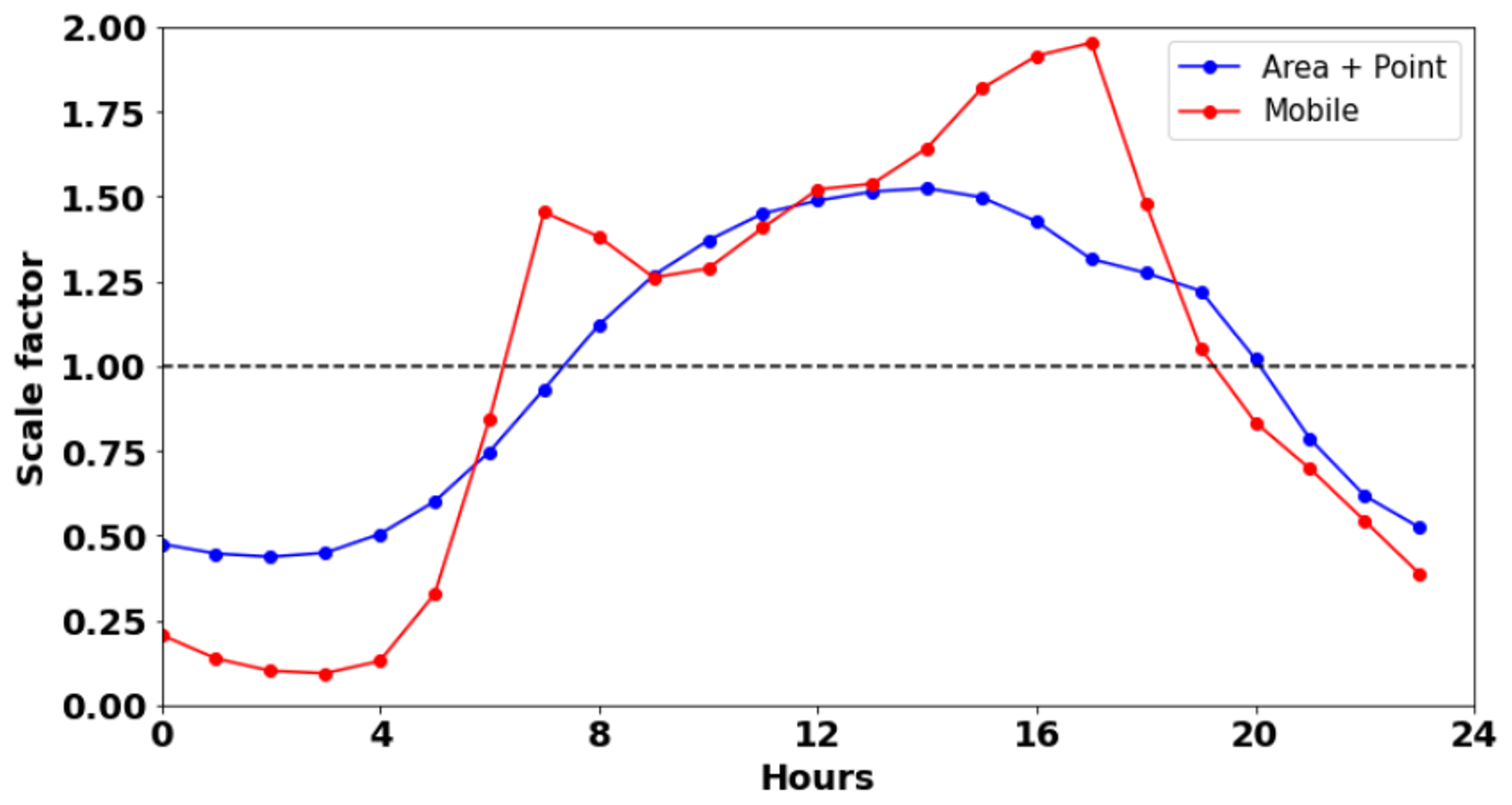
For our simulations over Seoul (presented in Sect. 5.1), we consider the diurnal variation in emissions using profiles based on area–point and mobile sectors developed for KORUS-AQ and described in application to modeling over Seoul by Jo et al. (2023). This is shown in Fig. 2 and predicts a pronounced increase in emissions with daytime activity and rush-hour peaks in the mobile emissions. As is discussed in Sect. 5.1, the assumed diurnal profile of model emissions can make a significant difference to the calculated TrC. Here, we include Fig. 2 showing the shape of the diurnal emissions to help in the interpretation of the results of Sect. 5.1 (particularly Fig. 10).
Quantitative comparison of satellite retrievals and model simulations requires consideration of the measurement sensitivity to the target quantity and the retrieval a priori assumptions. These can be accounted for by applying the retrieval averaging kernels that formally relate the retrieved quantity to the true atmosphere (Rodgers, 2000). For retrieval–model comparisons of trace gas TrC from GEMS-like sensors, the averaging kernels allow a retrieval-consistent TrC to be derived from the model trace gas profile or, alternatively, a model-consistent TrC to be calculated from the retrieval by substituting the retrieval a priori trace gas profile used in the AMF calculation for the model profile (e.g., Boersma et al., 2016). However, there are known issues with the GEMS V2.0 processing of the NO2 averaging kernels and the values reported in the operational data files, such that these should not be used as per guidance from NIER. The intention of the GEMS project is to remedy this issue with the next GEMS Version 3 release. Any independent or alternative reprocessing of the GEMS data to calculate averaging kernels is beyond the scope of this work. As a result, we are unable to perform quantitative model comparisons of the GEMS V2.0 products at this time, and the comparisons with MUSICAv0 presented in Sect. 5 should be considered mainly qualitative for now.
3.1 Hourly measurements
An example of the 10 GEMS daytime retrievals of NO2 TrC over Northeast Asia (25–45° N, 115–130° E) for the relatively clear day of 15 June 2023 is shown in Fig. 3. High NO2 is seen over the Beijing region and the industrial areas of the North China Plain. Pollution is also high over Shanghai and the Yangtze Delta with another hotspot over Seoul in South Korea. The most striking first impression of this GEO perspective on atmospheric composition is how large the temporal variation in the pollution is with respect to magnitude as well as how much the spatial distribution shifts on an hour-by-hour basis. In certain locations, changing cloud fields do not permit for all 10 possible retrievals to pass the data filters. However, the hourly observations do provide at least some measurements, thereby demonstrating an advantage of the GEO perspective. During the winter months when the Sun is low in the sky, there are fewer GEMS hourly retrievals. An example is shown in Fig. 4 for 30 January 2023 NO2 TrC over Northeast Asia. Compared with Fig. 3 (which uses the same color scale), the NO2 burden is considerably higher because of reduced NOx photochemical loss and NO2 TrC buildup during the day. This results in less diurnal variation compared with the summer months and is discussed in Sect. 5. The east–west data stripes evident in Fig. 3 exist in this data version across the domain, similar to the spurious across-track variability issue for OMI. Zhang et al. (2023) comment that this is likely associated with the specific scan modes of GEMS as well as periodically occurring bad pixels.
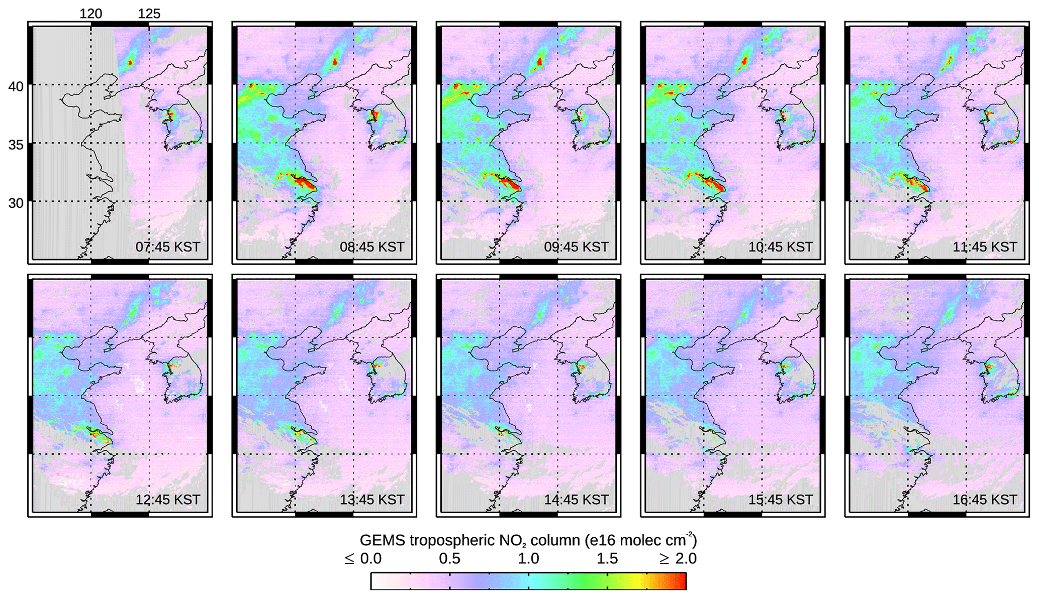
Figure 3Northeast Asia NO2 TrC hourly values for 15 June 2023. Observation times are Korean standard time (KST), i.e., coordinated universal time (UTC) plus 9 h. Gray indicates that no data were taken during nighttime or missing data due to clouds.
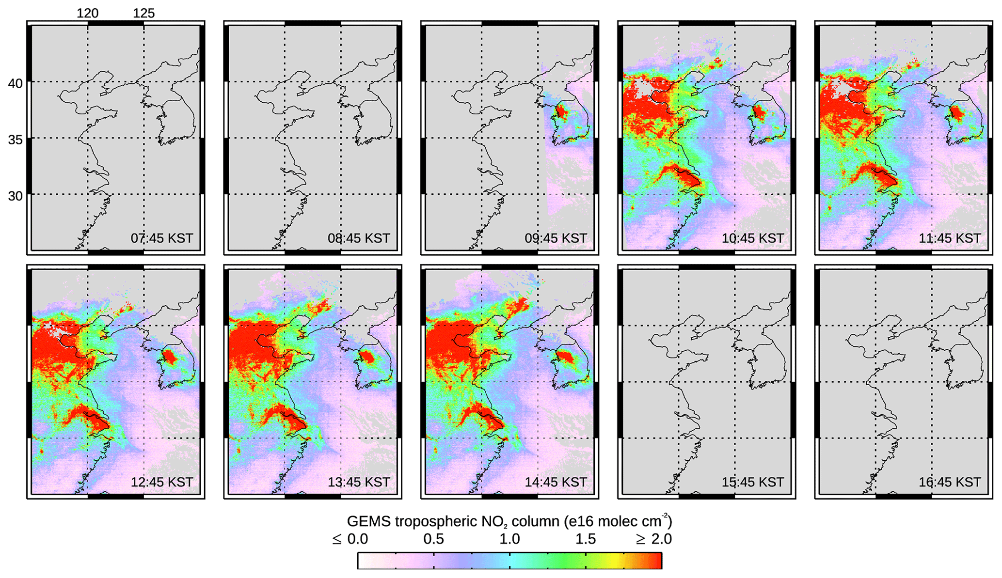
Figure 4Same as Fig. 3 but for 30 January 2023 NO2 TrC.
3.2 Quantifying GEMS NO2 diurnal variation
We have developed quantitative measures of the magnitude of the GEMS NO2 TrC daily absolute and relative variation. The first of these – ADV (absolute daily variation) – represents the absolute change in NO2 TrC for a given day and pixel location as sampled by multiple hourly GEMS observations:
where the pixel longitude and latitude are indexed by i and j, respectively, and k is the index of the GEMS hourly observation from 1 to n, with n being the number of useful cloud-free observations during the day. ADV is calculated for adjacent hourly observations, regardless of gaps due to missing data (gaps along a slope would have no effect on the resulting ADV value, although gaps where the slope changes sign may result in an underestimation). Figure 5 shows the monthly average of ADV for June 2023. Because this quantity depends on the number of useful cloud-free retrievals during the day, it is only calculated for days and locations for which there are at least five hourly observations; thus, it represents a lower bound on the total TrC change. No values are mapped east of ∼130° E, as there are too few daytime hourly observations at these locations. High variation usually coincides with locations of high TrC, such as industrial regions and cities, and illustrates the importance that time-resolved observations will have for characterizing changing NOx emissions and population pollution exposure. Chinese and Korean cities and Indian power facilities are particularly noticeable. Ship tracks between Hong Kong and Singapore as well as between Sri Lanka and the northern tip of Sumatra have been previously identified in GOME, SCIAMACHY, OMI, and TROPOMI NO2 data, among others (Beirle et al., 2004; Richter et al., 2004; Franke et al., 2009; Georgoulias et al., 2020). The ship tracks in Fig. 5 show diurnal variation, most likely because of horizontal dispersion with the increasing afternoon marine boundary layer. Averaging data temporally in this way at a given location reduces the contribution of transient emission or transport events that can produce significant day-to-day variation in the NO2 TrC. The averaged diurnal variation is then primarily dependent on emission and chemistry processes that occur on most days and, thus, indicates polluted urban regions in particular.
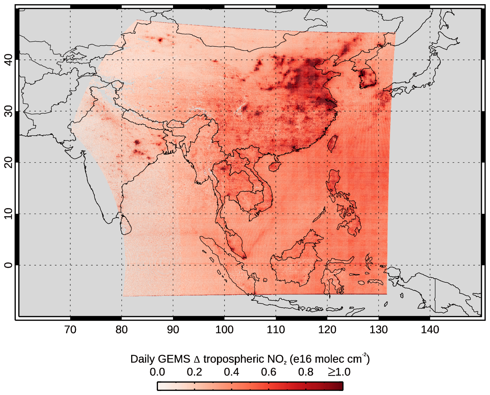
Figure 5Monthly average of the absolute daily variation (ADV) in the GEMS NO2 TrC for June 2023. The region east of ∼ 130° E is not mapped because only data points with five or more observations per day were included in this analysis.
A second measure that we consider relates the magnitude of the GEMS NO2 TrC relative daily variation (RDV) over multiple hourly observations with respect to the value of the single observation that would be obtained from a LEO instrument such as TROPOMI. For a particular day and pixel location, the absolute deviation in the day's hourly observed NO2 TrC relative to the observation at t=13:45 LT (closest to the TROPOMI overpass time) is calculated and normalized by the t = 13:45 value:
where t is the reference time (13:45 local standard time) and n is the number of observations at pixel location i,j excluding the observation acquired at the reference time. The daily RDV can then be averaged over the month, as shown for June 2023 in Fig. 6. The monthly averaged RDV is seen to be large, often > 50 % of the 13:45 LT value. The spatial distribution of RDV is similar to that of ADV shown in Fig. 5; however, in this case, it illustrates the diurnal uncertainties in emissions or exposure that might be expected from assuming estimates based on LEO observations. As for the absolute diurnal variation, because this quantity depends on the number of useful cloud-free retrievals during the day, it again represents a lower bound on the TrC variation. There are also no values at locations such as Japan and India where there is no 13:45 LT observation. The apparent high variation over the Pacific Ocean is a result of normalizing by the relatively low NO2 TrC values in this region.
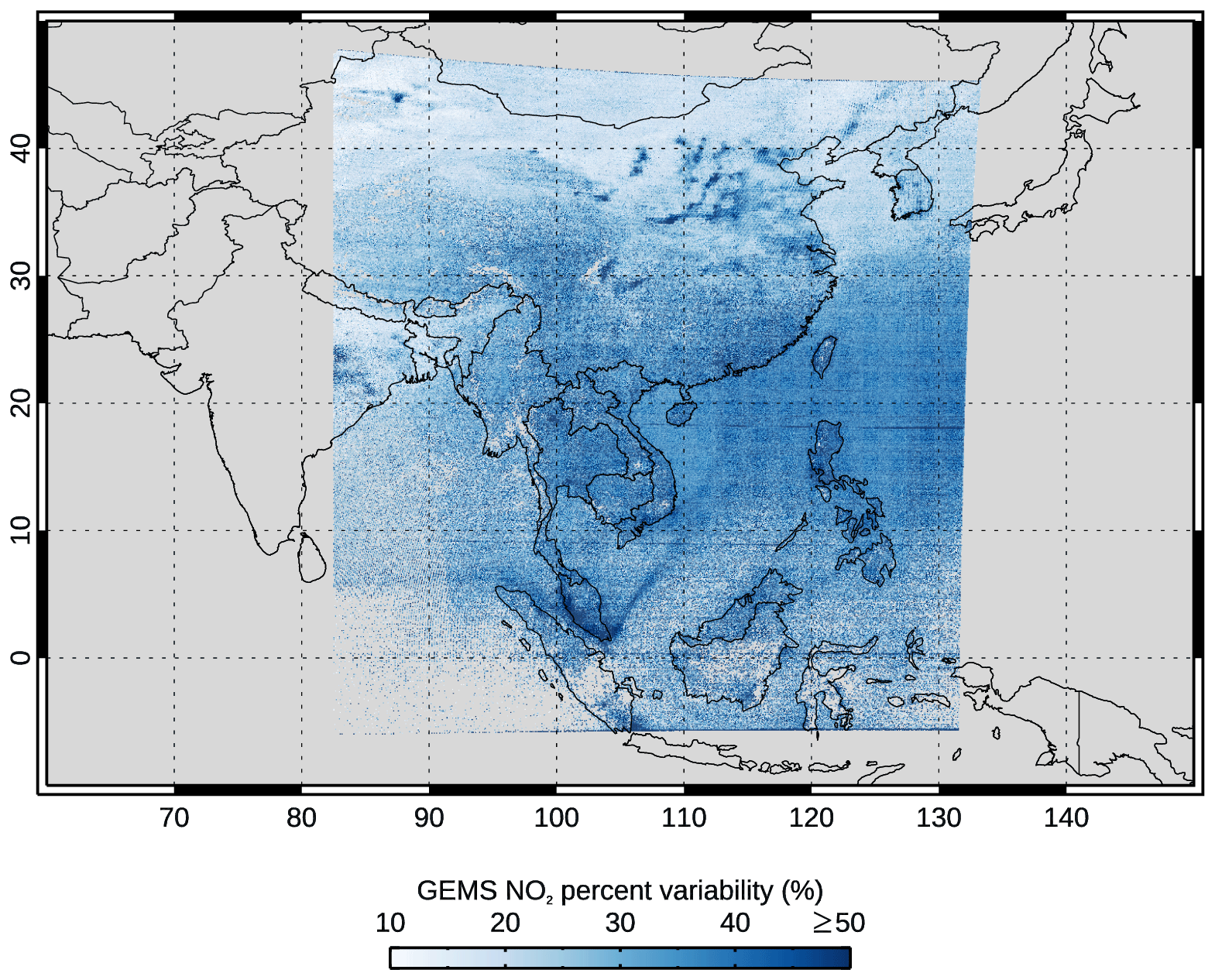
Figure 6The June 2023 monthly average of the GEMS NO2 TrC relative daily variation (RDV) with respect to the 13:45 LT observed value at each location. Regions west of 90° E and east of ∼ 130° E not mapped because there is no observation at 13:45 LT.
The January 2023 monthly average of the GEMS NO2 TrC ADV and RDV over the Northeast Asia region are shown in Figs. A1 and A2, respectively. In general, reduced winter photochemistry results in a smaller diurnal variation in January compared with June. However, over polluted regions, the ADV in NO2 TrC has similar values due to the higher January TrC. A noticeable region of high absolute daily change is also seen in Cambodia which requires further investigation but may be explained by fires. The Fig. A2 RDV map coverage is limited because the 13:45 LT observation is only available between longitudes 113 and 132° E.
3.3 GEMS regional- and local-scale NO2 diurnal variation time series
We have examined the time series of the GEMS NO2 TrC for various regions and seasons. Figure 7a shows the June 2023 time series spatially averaged over Northeast Asia (see Fig. 1 for the regional context). At this time of year, there are a maximum of 10 daylight hourly data points at the center of the GEMS FOR, with fewer points at the eastern and western edges. The number of hourly data points is further reduced by cloud filtering. On a day-to-day basis, the calculated average TrC appears noisy because of the changing amount and nonuniformity of cloud-free coverage, especially when polluted urban areas might be included in the spatial average on one day but not on the next. Because of this, the monthly time-averaged diurnal variation (Fig. 7b) is the quantity often considered. However, it is important to show the individual daily TrC after filtering for cloudy data to indicate the information that will usually be available for AQ applications. It should also be noted that cloudy missing points in the daily data tend to “flatten out” the apparent diurnal variation shown in the monthly time average; this suggests that this quantity be treated with care, as it may not capture the full dynamic range of the diurnal variation of individual days. Despite these considerations, a consistent diurnal cycle is seen on those days with multiple data points. This shows NO2 TrC decreasing through the morning hours, reaching a minimum in the early afternoon, and then increasing again late in the afternoon. Little difference is seen between weekdays and weekends at this spatial scale. As discussed in Sect. 5, we attribute this summer cycle primarily to photochemistry being the dominant driver of diurnal variation, as diurnal variation due to different local-scale emissions and meteorology is averaged out at this regional scale. This photochemical diurnal cycle is even more apparent when averaging over larger geographical regions, although different local times, solar zenith angles, and photolysis rates then complicate interpretation. A similar diurnal cycle is also seen in clean regions away from local sources or transported pollution plumes.
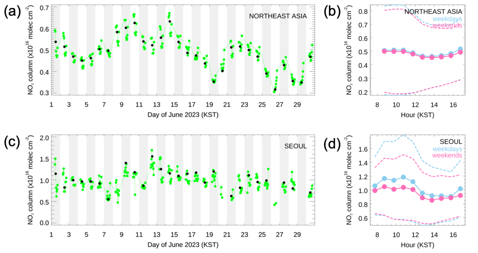
Figure 7The June 2023 diurnal NO2 TrC values spatially averaged over (a) the Northeast Asia region and (c) Seoul (see Fig. 1 for the regional context). Depending on cloud cover, there are up to 10 data points each day and no data at night. The black dot each day indicates the value closest to local noon. The monthly average weekday and weekend daily NO2 variation is also shown for (b) the Northeast Asia region and (d) Seoul. Note the high standard deviation (dashed lines).
The NO2 diurnal variation is less consistent at the local scale where, in addition to photochemistry, changing emissions and, more importantly, meteorology determine day-to-day variability. Figure 7c shows the time series spatially averaged over Seoul, South Korea (37–38° N, 126–127.5° E; see Fig. 1 for the regional context). Prior to the launch of GEMS, stagnation events over Seoul had been seen to cause a buildup of pollution during the day, leading to an afternoon maximum in NO2 TrC. This was observed by the Geostationary Trace gas and Aerosol Sensor Optimization (GeoTASO) aircraft spectrometer (Leitch et al., 2014) during the KORUS-AQ field campaign (Judd et al., 2018; Crawford et al., 2021). GEMS observations sometimes show this same diurnal pattern; however, as discussed in Sect. 5, they more often show a photochemical 10:00–11:00 LT morning maximum in NO2 contributed by urban emissions, followed by a decrease, and then a small late-afternoon increase, as shown in the monthly time-averaged diurnal variation in Fig. 7d. The weekend values indicate a similar diurnal cycle to weekdays with smaller TrC. We note that other work has shown large differences in the NO2 diurnal variation seen by GEMS between weekdays and weekends for different Asian cities (J. Park et al., 2022).
Reduced diurnal variation is shown in the January 2023 GEMS time series spatially averaged over the Northeast Asia and Seoul regions, as shown in Fig. 8. As noted above, the apparent large day-to-day differences in TrC result primarily from the varying number of cloud-free data that enter the spatial average, especially for the large-scale Northeast Asia region. Over both regions, an increase in TrC is usually observed during the day because of reduced winter photochemistry, as discussed in Sect. 5. This is the case for both weekdays and weekends, although the weekday TrC values are now clearly greater, indicating the persistence of NO2 resulting from higher weekday NOx emissions.
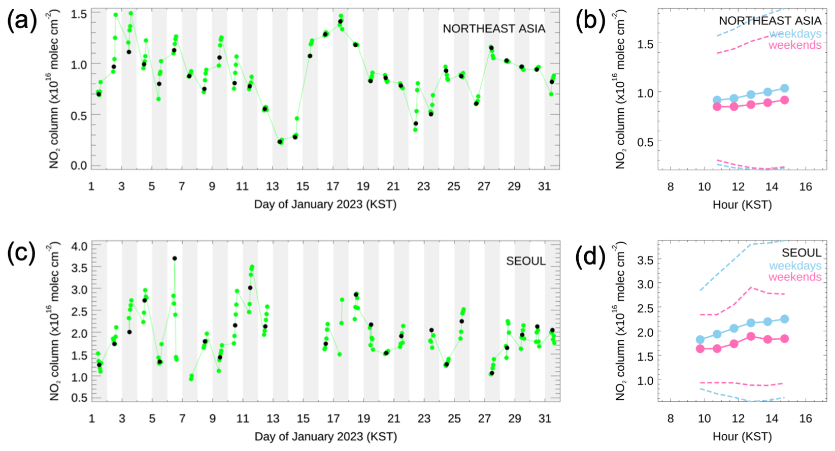
Figure 8Same as Fig. 7 but for January 2023 diurnal NO2 TrC. Depending on cloud cover, there are up to six data points each day and no data at night.
The Pandora instruments have emerged as the primary source of ground-based measurements for validation of GEMS NO2 and are also used extensively in TROPOMI validation (Kim et al., 2023). The advantage of these Sun photometers is that they provide column retrievals using the same spectral bands as GEMS and have similar measurement vertical sensitivities. The number of Pandora stations across Asia has been rising rapidly, and there are now 34 instruments contributing to the PGN. Here, we use Pandora measurements in Seoul as an independent indication of the diurnal variation.
For our study months, there were two PGN Pandora instruments making measurements within Seoul, at Seoul National University (Seoul-SNU, Pandora no. 149) close to Gwanaksan, and about 12 km to the north across the city and closer to the center at Yonsei University (Seoul-YN, Pandora no. 54). A comparison of the monthly time-averaged diurnal variation in the NO2 TotC measurements from GEMS and the Pandora instruments is shown in Fig. 9 for weekdays in June and January 2023. Figure 9 also indicates the monthly mean TROPOMI TotC NO2 at the local overpass time. We show Pandora NO2 TotC retrievals that use direct Sun measurements, rather than the multi-axis differential optical absorption spectroscopy (MAX-DOAS) measurements used for the TrC estimate. We also note that our model studies with the Whole Atmosphere Community Climate Model (WACCM) indicate that, over relatively polluted regions such as Seoul, the stratosphere contributes only a few percent NO2 to the total column. The GEMS and TROPOMI TotC values are calculated using a mean of retrievals within 5 km of the Pandora sites. For the Pandora–satellite measurement comparisons, we follow previous work (e.g., Judd et al., 2020; Lambert et al., 2023).
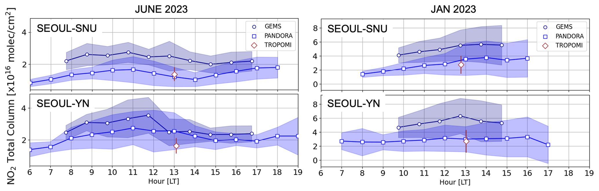
Figure 9GEMS, TROPOMI, and Pandora NO2 TotC values at Seoul-SNU and Seoul-YN, South Korea, for weekdays in June and January 2023. The GEMS and TROPOMI TotC are calculated using a mean of retrievals within 5 km of the Pandora sites.
The GEMS NO2 TotC values are larger overall than their Pandora counterparts with a higher bias in January than June. This positive bias has also been identified in comparisons with ground-based DOAS measurements with a median relative difference of +64 % and a correlation coefficient of 0.75 (Lange et al., 2024). This is contrary to what is usually found when comparing pixel-averaged satellite retrievals to local measurements that might capture small-scale high values (e.g., Herman et al., 2019). Tang et al. (2021) show that this representativeness error can account for a single Pandora measurement in Seoul being as much as ∼25 % higher than the GEMS retrieval for the corresponding pixel. Indeed Kim et al. (2023) found that GEMS V1.0 NO2 TotC measurements tend to be lower than their Pandora counterparts at less-polluted sites south of Seoul. Our own analysis at other Korean Pandora sites shows a much lower GEMS–Pandora bias in clean regions along with a small or flat diurnal variation that was also reported by Lange et al. (2024). We find that the GEMS V2.0 data positive bias is less than that of the previous V1.0 data but may still indicate retrieval issues to be addressed in future GEMS data releases. (A limited preview of the upcoming GEMS V3.0 NO2 data release with improved AMF calculation and StrC–TrC separation shows closer agreement with TROPOMI in summer but still an overestimation in winter.) The agreement between Pandora and TROPOMI is good at both sites and for both months, even though large negative (0 % to −50 %) biases in TROPOMI NO2 TotC have previously been reported (Verhoelst et al., 2021). We note here that we find no obvious measurement local time dependence in the GEMS–Pandora bias for Seoul or for the other Korean sites that we have examined.
Despite the positive GEMS bias, the agreement in the pattern of NO2 TotC diurnal variation captured by the Pandora instruments and the corresponding GEMS observations is reasonable at both Seoul sites in both months. The column amounts are lower in June than in January and indicate a morning NO2 maximum followed by a decrease through early afternoon and then a slight increase in the late afternoon. A clear rush-hour peak is not seen in these TotC measurements and is discussed further in Sect. 5.2. The sharp gradient in GEMS data over Seoul-YN in June between 12:00 and 13:00 LT is due to the value at 13:00 LT being anomalously low. This occurs because of the limited number of measurements (two or three per day) that meet the coincidence criteria with Pandora as well as the low number of cloud-free days in this month. The weekend values (not shown) have a flatter diurnal profile and less variation within each hour, although the average magnitude is only slightly smaller than weekdays. In January, both sites show a flat or increasing TrC during the day.
The Pandora NO2 TotC values are generally higher at Seoul-YN in June under the prevailing wind from the south at this time of year that blows more pollution from the city center toward this Pandora site. The opposite occurs during January when the prevailing wind is from the northeast. The same finding for Pandora–TROPOMI comparisons was previously reported by J.-U. Park et al. (2022). The GEMS satellite data capture some of this difference between the two sites and suggest that more work is needed to assess the capability the of GEMS to resolve pixel-scale urban variability for AQ applications.
5.1 Model NO2 diurnal variation
We have used the MUSICAv0 model to simulate the NO2 TrC for the same Northeast Asia and Seoul regions discussed above for June and January of 2023, and the model setup is as described in Sect. 2.4. For each case, we performed two simulations as a sensitivity test of the assumed anthropogenic diurnal emissions profile: the first assumes constant anthropogenic emissions during the day (labeled “Base”), whereas the second uses the KORUS-AQ area–point and mobile sector diurnal emissions profiles described in Sect. 2.4 and shown in Fig. 2 (labeled “Diurnal”). The average daily NO2 TrC diurnal variation for weekdays is shown in Fig. 10. The time windows corresponding to the periods during which GEMS retrievals are shown in Figs. 7 and 8 are indicated by the unshaded hours. As is noted in Sect. 2.4, there is an issue with the GEMS V2.0 NO2 averaging kernels which should not be used following the guidance of NIER. As a result, the discussion here comparing MUSICAv0 simulations to the GEMS retrievals presented in Sect. 3.3 should be considered to be mainly qualitative. However, we believe that the model is still able to provide insights into the drivers of the NO2 TrC diurnal variation and that presentation of these results is worthwhile as it sets the stage for more quantitative analysis with the next GEMS data version.
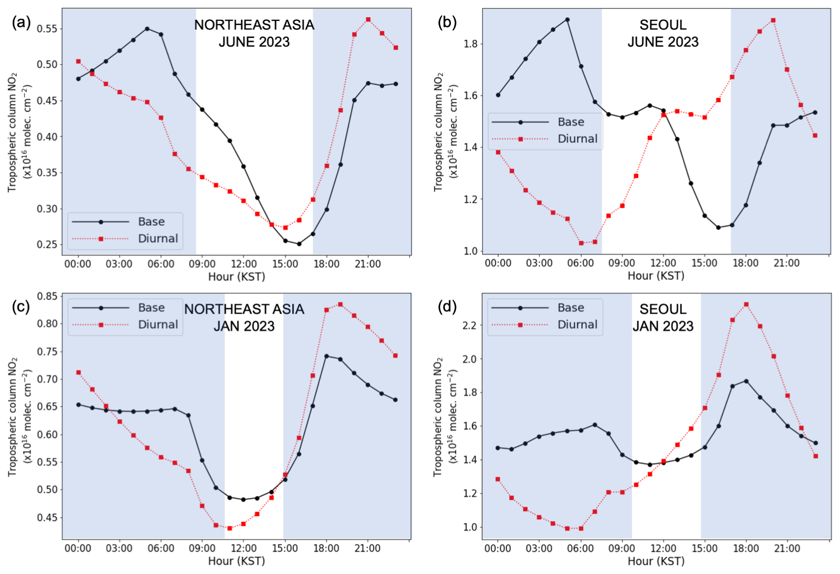
Figure 10MUSICAv0 NO2 TrC diurnal variation averaged over the Northeast Asia region (a, c) and Seoul (b, d) for weekdays in June 2023 (a, b) and January 2023 (c, d). The time windows corresponding to the periods during which GEMS retrievals are shown in Figs. 7 and 8 are indicated by the unshaded hours. The Base simulation assumes a constant diurnal emissions profile, whereas the Diurnal simulation uses the diurnal emissions profile discussed in Sect. 2.4 and shown in Fig. 2.
5.2 The role of emissions
We first consider the model results spatially averaged over the Northeast Asia study region and temporally averaged for weekdays in the months of June and January 2023 (Fig. 10a and c, respectively). The model patterns for the NO2 TrC diurnal variation are generally similar to the corresponding GEMS (Figs. 7b and 8b). However, as the model does not include cloud cover and reproduces a consistent daily pattern, the dynamic range of the diurnal variation is greater than the averaged GEMS data. The GEMS data are biased high relative to the model in both months with the difference being largest in January. This may be a GEMS V2.0 retrieval issue, as noted above, and/or an underestimation of NOx emissions in MUSICAv0. At this regional scale, the diurnal variation is similar for both the Base and Diurnal simulations, despite the very different anthropogenic diurnal emissions profiles, and suggests that photochemistry is the main driver. However, the magnitude of the diurnal variation during the GEMS retrieval window does depend on the emissions profile, ranging from 25 %–50 % in June to 6 %–17 % in January. We note that the GEMS NO2 TrC daily relative variation over Northeast Asia for June and January 2023 (Figs. 6 and A2, respectively) falls at the bottom of these ranges, suggesting that further work is needed to understand the greater model variation. The emissions profile also affects the local hour of the minimum NO2 TrC and is about 1 h earlier in the Diurnal case, which matches better with GEMS.
Over the Seoul region, the difference in NO2 diurnal variation between the Base and Diurnal simulations is large, especially in June (Fig. 10b). For the Base simulation in June, the shape of the diurnal variation shows a similar photochemical cycle to that described above for the Northeast Asia region. A difference is seen in that there is a NO2 morning peak around 10:00–11:00 LT, a decrease through midday, and then an afternoon minimum, like the diurnal variation seen in the corresponding GEMS data (Fig. 7d). This is discussed further in the next section. In contrast, the Diurnal simulation shows a very different NO2 buildup throughout the day and reflects the shape of the NOx diurnal emissions profile used in the model; however, the pronounced rush-hour peaks seen in Fig. 2 are not evident in the NO2 TrC average, even though they do clearly show up in the calculated surface concentration (not shown). Nevertheless, the fact that the average GEMS NO2 diurnal variation shown in Fig. 7d more closely resembles the constant NOx emissions of the Base simulation suggests that the hourly changes in the emissions profile may not actually be as large as indicated in Fig. 2. In January, both simulations show increasing TrC during the GEMS retrieval window, in agreement with the GEMS data in Fig. 8d. These simulations indicate that the modeled diurnal variation at the city scale will be very dependent on the diurnal profile of the assumed emissions, and the accurate characterization of the assumed emissions will be an important part of effectively using the hourly observations from GEO.
5.3 The role of chemistry
The underlying photochemical cycle is explained by considering the June 2023 Base simulation TrC NOx budget analysis shown in Fig. 11a for Seoul. After a buildup of NO2 during nighttime, photolysis begins with sunrise at 05:00 LT, and the morning decrease is mirrored by the increase in NO with the rise in the NO2 photolysis rate () curve with increasing solar elevation. Although the NOx ratio is in a photochemical steady state on timescales of minutes, the diurnal change in solar irradiance drives a continual change in the ratio through the day. It should also be remembered that this calculation is for the TrC relevant to the GEMS retrieval and is, therefore, representative of a vertically weighted average, rather than surface values. After 10:00 LT, NO loss with the buildup of O3 pushes the NOx ratio toward NO2 at the same time that NOx is lost to the nitrogen reservoirs HNO3, and to a lesser extent, PAN. This balance results in a slight peak in NO2 around 11:00 LT; a continued decline due to NOx loss is then seen until the minimum at 16:00 LT. Decreasing photolysis results in a subsequent NO2 increase into nighttime with continuing NOx emissions. The underlying chemistry is similar for the corresponding June Diurnal simulation (not shown) only in this case, as the increasing NOx emissions during the day result in the replacement of most of the atmospheric NOx that is lost to the nitrogen reservoirs with a consequent gradual buildup of NO2.
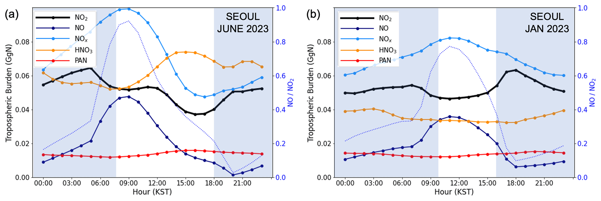
Figure 11MUSICAv0 (a) June and (b) January 2023 average daily NOx TrC budget analysis over Seoul assuming constant anthropogenic emissions during the day (Base simulation). The time windows corresponding to the periods during which GEMS retrievals are shown in Figs. 7 and 8 are indicated by the unshaded hours.
In the January 2023 Base simulation shown in Fig. 11b, atmospheric NOx shows less variation under conditions of lower photolysis, lower O3, and less daytime conversion to HNO3. The NOx ratio depends mainly on the change in the curve under conditions of limited photochemical activity, resulting in a 11:00 LT NO maximum and NO2 minimum (as shown in Fig. 10d). In the January Diurnal simulation (not shown), NO2 again builds up during the day following the increasing NOx emissions.
5.4 The role of meteorology
The MUSICAv0 monthly averaged daily NO2 TrC diurnal variation over Seoul (shown in Fig. 10b and d) results from averaging the diurnal variation during each day of June and January 2023. As noted before, the Base simulation usually shows an afternoon minimum, whereas the Diurnal simulation shows a buildup of pollution during the day and produces a late-afternoon NO2 peak. Both simulations indicate that day-to-day changes in the NO2 TrC magnitude depend primarily on meteorology. This is illustrated in Fig. 12, which shows the correlation of the average model NO2 TrC during the day with the model surface-layer wind (usually around ∼ 120 m) and also indicates the average wind direction over the city. This is shown separately in plots for June and January calculations for the 2 years of 2022 and 2023 together. For both months, there is a clear anticorrelation (R about −0.7) of NO2 TrC and wind speed. In June, the prevailing wind over Seoul is usually from the south. Shifts to winds from the west result in a lower wind speed and stagnant conditions over the city that permit a buildup of pollution, and this is reflected in the TrC value. Similar anticorrelation is seen in January, although the winds over Seoul during winter are mostly from the northwest and an occasional change to a weak anticyclonic pattern results in a low wind speed and NO2 TrC buildup.
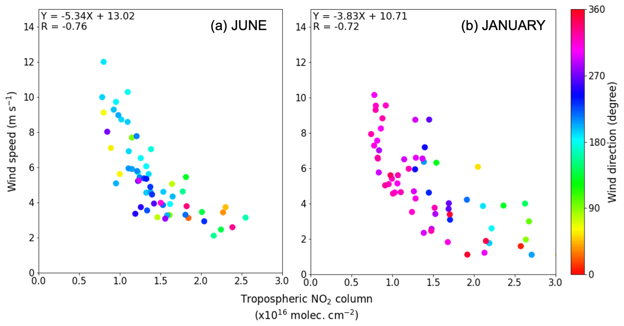
Figure 12Scatter plot of the MUSICAv0 average daily NO2 TrC compared to the magnitude and direction of the prevailing model surface-layer wind (usually around ∼120 m) over Seoul for June and January combined data for the 2 years of 2022 and 2023 assuming constant anthropogenic emissions during the day (Base case).
A similar analysis for the modeled diurnal variation absolute daily change in NO2 TrC discussed in Sect. 3.2 does not show clear correlation (R of about −0.35) with wind speed in either month over Seoul. This suggests that the emission and chemistry processes discussed above are most important in determining the local diurnal variation and do not necessarily require stagnant meteorological conditions. We note that Yang et al. (2023b) did see correspondence between a low model wind speed and higher winter NO2 diurnal variation; therefore, further investigation using wind measurements would be useful. We have also examined the contribution of incoming transport to the NO2 TrC, although Seoul is unlikely to be a generally representative city in this respect, as it is large, fairly isolated, and has very high local NOx emissions. Upwind GEMS NO2 TrC values are usually about 3–4 times lower than the values retrieved over the city and have relatively flat diurnal variation, suggesting that incoming transport contributions to the Seoul NO2 TrC diurnal or day-to-day variations will be small. This might not be the case for longer-lived pollutants or when considering concentrations at a specific altitude, such as in the free troposphere (Jordan et al., 2020). In cleaner regions downwind of Seoul, the GEMS NO2 TrC measurements do show higher values because of plumes following a high-pollution day over the city. Understanding the role of meteorology is going to be important for our next step of relating the satellite retrievals of TrC to surface concentrations. Results from KORUS-AQ showed that meteorology and PBL dynamics play a large role in determining the extent to which the satellite and ground-based in situ views of pollutant diurnal variation can be reconciled (Crawford et al., 2021).
Over the last 20 years, LEO observations have provided satellite measurements of pollutants in the atmosphere with increasing scientific utility, mainly at continental to global and weekly to seasonal scales. New-generation LEO instruments (e.g., IASI, CrIS, and TROPOMI) have allowed for refinements in both the spatial and temporal resolutions, to city and daily scales. The GEO satellite perspective, with hourly high-spatial-resolution measurements, represents another major step forward, especially with respect to the capability to understand how AQ processes change diurnally at the local scale. The main conclusions of this work are as follows:
-
GEMS observations show that NO2 TrC diurnal variation can be large (>50 % of the TrC) and varies by location, being higher in polluted environments. The NO2 distribution is seen to change hourly and can be quite different from what would be seen in a once-a-day LEO observation. This is demonstrated by the quantitative measures of diurnal variation that we have presented, such as the monthly average of the absolute daily change in TrC or the diurnal relative variation in TrC. Along with enabling one or more observations within a day under changing cloud conditions, this demonstrates the advantages of the GEO perspective.
-
Regionally averaging GEMS NO2 TrC data emphasizes the diurnal variation due to chemistry, as local-scale variability due to emissions and meteorology is minimized. Temporally averaging the data for a particular hour over several days or weeks emphasizes persistent chemistry and emissions patterns while minimizing meteorological variability.
-
In June, NO2 photochemistry is an important driver of diurnal variation, especially at the regional scale. At the local scale, the NO2 magnitude and diurnal variation patterns change on a day-to-day basis, showing the impact of emissions and meteorology. In January, NO2 columns are higher and diurnal variation is lower because of reduced photochemistry.
-
Initial comparisons with Pandora measurements over Seoul show a reduction in the GEMS V2.0 positive bias with respect to GEMS V1.0 and reasonable agreement with respect to the shape of diurnal variation. The GEMS differences between the two Pandora sites suggest the possibility of resolving pixel-scale urban variation for AQ applications.
-
Model simulations show high sensitivity to the assumed diurnal emissions profile, especially at the local scale. This will have consequences ranging from the assumed NO2 vertical profile used in retrieval AMF calculations to the background model field used for GEMS data assimilation.
-
The model indicates an anticorrelation between the surface-layer wind speed and the daily mean NO2 TrC, the latter of which can build up under stagnant conditions.
This work has concentrated on understanding the diurnal variation in the GEMS NO2 TrC retrievals with a CTM. In combination with ground-based remote sensing and in situ measurements, the next step will be to connect the GEO and LEO satellite-derived columns (not only of NO2 but also other trace gas species, particularly O3 and HCHO) to the surface-level concentrations. This will allow the derivation of top-down diurnal emissions profiles that can be applied to the standard bottom-up emissions inventories. Including this diurnal variation is going to be important for determining true pollutant exposure levels for AQ studies. The work presented here also provides a path for investigating similar NO2 diurnal cycles in the new TEMPO data over North America, and later over Europe with Sentinel-4.
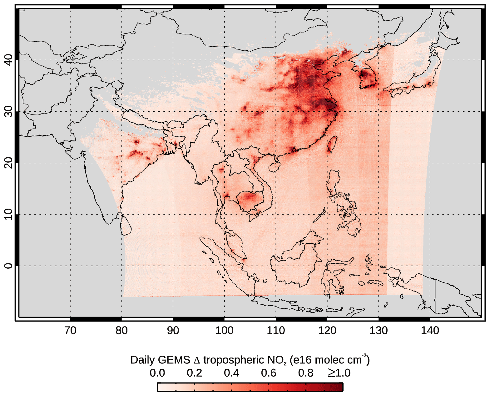
Figure A1Monthly average of the absolute daily variation (ADV) in the GEMS NO2 TrC for January 2023. Data points with three or more observations per day were included in this analysis.
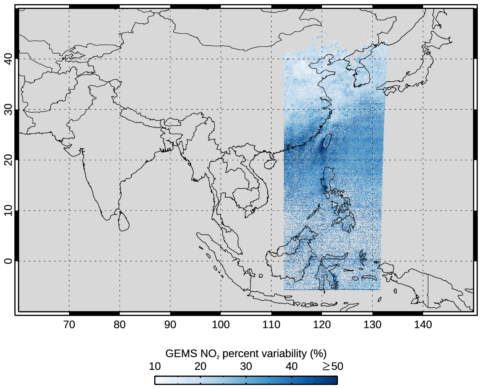
Figure A2The January 2023 monthly average of the GEMS NO2 TrC relative daily variation (RDV) with respect to the 13:45 LT observed value at each location. Regions west of about 113° E and east of about 132° E are not mapped due to the lack of observations at 13:45 LT.
MUSICAv0 (Pfister, 2020) is a configuration of CESM2.2, which is an open-source community model available from https://github.com/ESCOMP/CESM (last access: 14 February 2024). The code version used for this work and the modifications to include the diurnal cycle of anthropogenic emissions, grid information files, and simulation results are available at https://doi.org/10.5281/zenodo.8044736 (Jo, 2023).
The GEMS L2 NO2 V2.0 data (NIER, 2024) can be obtained via application to NIER (https://nesc.nier.go.kr/en/html/cntnts/91/static/page.do). The Pandora NO2 data are available from the Pandonia Global Network data archive (http://data.pandonia-global-network.org/; PGN, 2024). The TROPOMI NO2 data are publicly available from the NASA Earthdata portal (https://search.earthdata.nasa.gov/; Earthdata, 2024).
DPE: conceptualization; DPE, SMA, DSJ, and IO: methodology; DPE, SMA, DSJ, and IO: formal analysis; SMA, DSJ, IO, HL, JP, and HH: data curation; SMA, IO, JK, HL, JP, and HH: validation; SMA, DSJ, and IO: visualization; DPE, HMW, and LKE: supervision; DPE and SMA: writing – original draft preparation; SMA, DSJ, IO, LKE, JJO, HMW, JK, HL, JP, and HH: writing – review and editing.
At least one of the (co-)authors is a member of the editorial board of Atmospheric Chemistry and Physics. The peer-review process was guided by an independent editor, and the authors also have no other competing interests to declare.
Publisher's note: Copernicus Publications remains neutral with regard to jurisdictional claims made in the text, published maps, institutional affiliations, or any other geographical representation in this paper. While Copernicus Publications makes every effort to include appropriate place names, the final responsibility lies with the authors. Regarding the maps used in this paper, please note that Figs. 1, 5, 6, A1, and A2 contain disputed territories.
This article is part of the special issue “GEMS: first year in operation (AMT/ACP inter-journal SI)”. It is not associated with a conference.
This material is based upon work supported by the National Center for Atmospheric Research, which is a major facility sponsored by the National Science Foundation (under cooperative agreement no. 1852977). Duseong S. Jo was supported by the New Faculty Startup Fund from Seoul National University. The authors would like to acknowledge high-performance computing support from Cheyenne (https://doi.org/10.5065/D6RX99HX; Computational and Information Systems Laboratory, 2019), provided by NSF NCAR's Computational and Information Systems Laboratory, sponsored by the National Science Foundation. We are also grateful to Doug Kinnison (NCAR/ACOM) for providing the WACCM simulations and discussing stratospheric NO2. Finally, we wish to thank the TROPOMI and PGN teams for observational data.
This research has been supported by the Smithsonian Astrophysical Observatory (grant no. SV3-83021).
This paper was edited by Bryan N. Duncan and reviewed by two anonymous referees.
Bazalgette Courrèges-Lacoste, G., Sallusti, M., Bulsa, G., Bagnasco, G., Veihelmann, B., Riedl, S., Smith, D. J., and Maurer, R.: The Copernicus Sentinel 4 mission: A geostationary imaging UVN spectrometer for air quality monitoring, Proc. SPIE 10423, Sensors, Systems, and Next-Generation Satellites XXI, 10423, https://doi.org/10.1117/12.2282158, 2017.
Beirle, S., Platt, U., von Glasow, R., Wenig, T., and Wagner, T.: Estimate of nitrogen oxide emissions from shipping by satellite remote sensing, Geophys. Res. Lett., 31, L18102, https://doi.org/10.1029/2004GL020312, 2004.
Bey, I., Jacob, D. J., Yantosca, R. M., Logan, J. A., Field, B., Fiore, A. M., Li, Q., Liu, H., Mickley, L. J., and Schultz, M.: Global modeling of tropospheric chemistry with assimilated meteorology: Model description and evaluation, J. Geophys. Res., 106, 23073–23096, 2001.
Boersma, K. F., Vinken, G. C. M., and Eskes, H. J.: Representativeness errors in comparing chemistry transport and chemistry climate models with satellite UV–Vis tropospheric column retrievals, Geosci. Model Dev., 9, 875–898, https://doi.org/10.5194/gmd-9-875-2016, 2016.
Brasseur, G., Orlando, J. J., and Tyndall, G. S. (Eds.): Atmospheric chemistry and global change, Oxford University Press, New York, ISBN: 9780195105216, 1999.
Bucsela, E. J., Krotkov, N. A., Celarier, E. A., Lamsal, L. N., Swartz, W. H., Bhartia, P. K., Boersma, K. F., Veefkind, J. P., Gleason, J. F., and Pickering, K. E.: A new stratospheric and tropospheric NO2 retrieval algorithm for nadir-viewing satellite instruments: applications to OMI, Atmos. Meas. Tech., 6, 2607–2626, https://doi.org/10.5194/amt-6-2607-2013, 2013.
CEOS: A geostationary satellite constellation for observing global air quality: An international path forward, CEOS atmospheric composition constellation executive summary, https://ceos.org/observations/documents/AC-VC_Geostationary-Cx-for-Global-AQ-final_Apr2011.pdf (last access: 2 August 2024), 2019.
Choi, Y., Kim, G., Kim, B., and Kwon, M.: Geostationary Environment Monitoring Spectrometer (GEMS) algorithm theoretical basis document cloud retrieval algorithm, Ministry of Environment, https://nesc.nier.go.kr/en/html/satellite/doc/doc.do (last access: 2 August 2024), 2020.
Clerbaux, C., Boynard, A., Clarisse, L., George, M., Hadji-Lazaro, J., Herbin, H., Hurtmans, D., Pommier, M., Razavi, A., Turquety, S., Wespes, C., and Coheur, P.-F.: Monitoring of atmospheric composition using the thermal infrared IASI/MetOp sounder, Atmos. Chem. Phys., 9, 6041–6054, https://doi.org/10.5194/acp-9-6041-2009, 2009.
Computational and Information Systems Laboratory: Cheyenne: HPE/SGI ICE XA System (University Community Computing), National Center for Atmospheric Research, Boulder, CO, https://doi.org/10.5065/D6RX99HX, 2019.
Crawford, J. H., Ahn, J.-Y., Al-Saadi, J., Chang, L., Emmons, L. K., Kim, J., Lee, G., Park, J.-H., Park, R. J., Woo, J. H., Song, C.-K., Hong, J.-H., Hong, Y.-D., Lefer, B. L., Lee, M., Lee, T., Kim, S., Min, K.-E., Yum, S. S., and Shin, H. J.: The Korea–United States Air Quality (KORUS-AQ) field study, Elementa: Science of the Anthropocene, 9, 00163, https://doi.org/10.1525/elementa.2020.00163, 2021.
Crippa, M., Solazzo, E., Huang, G., Guizzardi, D., Koffi, E., Muntean, M., Schieberle, C., Friedrich, R., and Janssens-Maenhout, G.: High resolution temporal profiles in the Emissions Database for Global Atmospheric Research, Scientific Data, 7, 121, https://doi.org/10.1038/s41597-020-0462-2, 2020.
Curier, R. L., Kranenburg, R., Segers, A. J. S., Timmermans, R. M. A., and Schaap, M.: Synergistic use of OMI NO2 tropospheric columns and LOTOS–EUROS to evaluate the NOx emission trends across Europe, Remote Sens. Environ., 149, 58–69, https://doi.org/10.1016/j.rse.2014.03.032, 2014.
de Foy, B. and Schauer, J. J.: An improved understanding of NOx emissions in South Asian megacities using TROPOMI NO2 retrievals, Environ. Res. Lett., 17, 024006, https://doi.org/10.1088/1748-9326/ac48b4, 2022.
de Ruyter de Wildt, M., Eskes, H., and Boersma, K. F.: The global economic cycle and satellite-derived NO2 trends over shipping lanes, Geophys. Res. Lett., 39, L01802, https://doi.org/10.1029/2011GL049541, 2012.
Duncan, B., Yoshida, Y., de Foy, B., Lamsal, L., Streets, D., Lu, Z., Pickering, K., and Krotkov, N.: The observed response of Ozone Monitoring Instrument (OMI) NO2 columns to NOx emission controls on power plants in the United States: 2005–2011, Atmos. Environ., 81, 102–111, https://doi.org/10.1016/j.atmosenv.2013.08.068, 2013.
Duncan, B. N., Lamsal, L. N., Thompson, A. M., Yoshida, Y., Lu, Z., Streets, D. G., Hurwitz, M. M., and Pickering, K. R.: A space-based, high-resolution view of notable changes in urban NOx pollution around the world (2005–2014), J. Geophys. Res.-Atmos., 121, 976–996, https://doi.org/10.1002/2015JD024121, 2016.
Earthdata: NASA portal, https://search.earthdata.nasa.gov/, last access: 14 February 2024.
Emmons, L. K., Schwantes, R. H., Orlando, J. J., Tyndall, G., Kinnison, D., Lamarque, J., Marsh, D., Mills, M. J., Tilmes, S., Bardeen, C., Buchholz, R. R., Conley, A., Gettelman, A., García, R., Simpson, I., Blake, D. R., Meinardi, S., and Pétron, G.: The Chemistry Mechanism in the Community Earth System Model Version 2 (CESM2), J. Adv. Model. Earth Sy., 12, e2019MS001882, https://doi.org/10.1029/2019ms001882, 2020.
Fishman, J., Iraci, L. T., Al-Saadi, J., Chance, K., Chavez, F., Chin, M., Coble, P., Davis, C., DiGiacomo, P. M., Edwards, D., Eldering, A., Goes, J., Herman, J., Hu, C., Jacob, D. J., Jordan, C., Kawa, S. R., Key, R., Liu, X., and Lohrenz, S.: The United States' next generation of atmospheric composition and coastal ecosystem measurements: NASA's GEOstationary Coastal and Air Pollution Events (GEO-CAPE) mission, B. Am. Meteorol. Soc., 93, 1547–1566, https://doi.org/10.1175/BAMS-D-11-00201.1, 2012.
Franke, K., Richter, A., Bovensmann, H., Eyring, V., Jöckel, P., Hoor, P., and Burrows, J. P.: Ship emitted NO2 in the Indian Ocean: comparison of model results with satellite data, Atmos. Chem. Phys., 9, 7289–7301, https://doi.org/10.5194/acp-9-7289-2009, 2009.
Geddes, J. A., Martin, R. V., Bucsela, E. J., McLinden, C. A., and Cunningham, D. J. M.: Stratosphere–troposphere separation of nitrogen dioxide columns from the TEMPO geostationary satellite instrument, Atmos. Meas. Tech., 11, 6271–6287, https://doi.org/10.5194/amt-11-6271-2018, 2018.
Georgoulias, A. K., Boersma K. F., van Vliet, J., Zhang, X., van der A, R., Zanis, P., and de Laat, J.: Detection of NO2 pollution plumes from individual ships with the TROPOMI/S5P satellite sensor, Environ. Res. Lett., 15, 124037–124037, https://doi.org/10.1088/1748-9326/abc445, 2020.
Goldberg, D. L., Anenberg, S. C., Kerr, G. H., Mohegh, A., Lu, Z., and Streets, D. G.: TROPOMI NO2 in the United States: A detailed look at the annual averages, weekly cycles, effects of temperature, and correlation with surface NO2 concentrations, Earths Future, 9, e2020EF001665, https://doi.org/10.1029/2020ef001665, 2021.
Griffin, D., McLinden, C. A., Dammers, E., Adams, C., Stockwell, C. E., Warneke, C., Bourgeois, I., Peischl, J., Ryerson, T. B., Zarzana, K. J., Rowe, J. P., Volkamer, R., Knote, C., Kille, N., Koenig, T. K., Lee, C. F., Rollins, D., Rickly, P. S., Chen, J., Fehr, L., Bourassa, A., Degenstein, D., Hayden, K., Mihele, C., Wren, S. N., Liggio, J., Akingunola, A., and Makar, P.: Biomass burning nitrogen dioxide emissions derived from space with TROPOMI: methodology and validation, Atmos. Meas. Tech., 14, 7929–7957, https://doi.org/10.5194/amt-14-7929-2021, 2021.
Guenther, A. B., Jiang, X., Heald, C. L., Sakulyanontvittaya, T., Duhl, T., Emmons, L. K., and Wang, X.: The Model of Emissions of Gases and Aerosols from Nature version 2.1 (MEGAN2.1): an extended and updated framework for modeling biogenic emissions, Geosci. Model Dev., 5, 1471–1492, https://doi.org/10.5194/gmd-5-1471-2012, 2012.
Han, Y., Revercomb, H., Cromp, M., Gu, D., Johnson, D., Mooney, D., Scott, D., Strow, L., Bingham, G., Borg, L., Chen, Y., DeSlover, D., Esplin, M., Hagan, D., Jin, X., Knuteson, R., Motteler, H., Predina, J., Suwinski, L., and Taylor, J.: Suomi NPP CrIS measurements, sensor data record algorithm, calibration and validation activities, and record data quality, J. Geophys. Res.-Atmos., 118, 12734–12748, https://doi.org/10.1002/2013jd020344, 2013.
Herman, J., Abuhassan, N., Kim, J., Kim, J., Dubey, M., Raponi, M., and Tzortziou, M.: Underestimation of column NO2 amounts from the OMI satellite compared to diurnally varying ground-based retrievals from multiple PANDORA spectrometer instruments, Atmos. Meas. Tech., 12, 5593–5612, https://doi.org/10.5194/amt-12-5593-2019, 2019.
Herman, J. R., Cede, A., Spinei, E., Mount, G. H., Tzortziou, M., and Abuhassan, N.: NO2 column amounts from ground-based Pandora and MFDOAS spectrometers using the direct-sun DOAS technique: Intercomparisons and application to OMI validation, J. Geophys. Res., 114, D13307, https://doi.org/10.1029/2009jd011848, 2009.
Huber, D. E., Steiner, A. L., and Kort, E. A.: Daily cropland soil NOx emissions identified by TROPOMI and SMAP, Geophys. Res. Lett., 47, e2020GL089949, https://doi.org/10.1029/2020gl089949, 2020.
Jang, Y., Lee, Y., Kim, J., Kim, Y. H., and Woo, J.: Improvement China point source for improving bottom-up emission inventory, Asia-Pac. J. Atmos. Sci., 56, 107–118, https://doi.org/10.1007/s13143-019-00115-y, 2019.
Jo, D.: MUSICAv0 results for Jo et al. (2023) in JAMES, Version v1, Zenodo [data set], https://doi.org/10.5281/zenodo.8044736, 2023.
Jo, D. S., Emmons, L. K., Callaghan, P., Tilmes, S., Woo, J., Kim, Y. H., Kim, J., Granier, C., Soulié, A., Doumbia, T., Darras, S., Buchholz, R. R., Simpson, I. J., Blake, D. R., Wisthaler, A., Schroeder, J., Fried, A., and Kanaya, Y.: Comparison of urban air quality simulations during the KORUS-AQ campaign with regionally refined versus global uniform grids in the MUlti-Scale Infrastructure for Chemistry and Aerosols (MUSICA) Version 0, J. Adv. Model. Earth Sy., 15, e2022MS003458, https://doi.org/10.1029/2022ms003458, 2023.
Jordan, C. E., Crawford, J. H., Beyersdorf, A. J., Eck, T. F., Halliday, H. S., Nault, B. A., Chang, L.-S., Park, J., Park, R., Lee, G., Kim, H., Ahn, J.-Y., Cho, S., Shin, H. J., Lee, J. H., Jung, J., Kim, D.-S., Lee, M., Lee, T., Whitehill, A., Szykman, J., Schueneman, M. K., Campuzano-Jost, P., Jimenez, J. L., DiGangi, J. P., Diskin, G. S., Anderson, B. E., Moore, R. H., Ziemba, L. D., Fenn, M. A., Hair, J. W., Kuehn, R. E., Holz, R. E., Chen, G., Travis, K., Shook, M., Peterson, D. A., Lamb, K. D., and Schwarz, J. P.: Investigation of factors controlling PM2.5 variability across the South Korean Peninsula during KORUS-AQ, Elementa: Science of the Anthropocene, 8, 28, https://doi.org/10.1525/elementa.424, 2020.
Judd, L. M., Al-Saadi, J. A., Valin, L., Pierce, R. B., Yang, K., Janz, S. J., Kowalewski, M. G., Szykman, J., Tiefengraber, M., and Müller, M.: The dawn of geostationary air quality monitoring: Case studies from Seoul and Los Angeles, Front. Environ. Sci., 6, 85, https://doi.org/10.3389/fenvs.2018.00085, 2018.
Judd, L. M., Al-Saadi, J. A., Szykman, J. J., Valin, L. C., Janz, S. J., Kowalewski, M. G., Eskes, H. J., Veefkind, J. P., Cede, A., Mueller, M., Gebetsberger, M., Swap, R., Pierce, R. B., Nowlan, C. R., Abad, G. G., Nehrir, A., and Williams, D.: Evaluating Sentinel-5P TROPOMI tropospheric NO2 column densities with airborne and Pandora spectrometers near New York City and Long Island Sound, Atmos. Meas. Tech., 13, 6113–6140, https://doi.org/10.5194/amt-13-6113-2020, 2020.
Kim, B.-R., Kim, G., Cho, M., Choi, Y.-S., and Kim, J.: First results of cloud retrieval from the Geostationary Environmental Monitoring Spectrometer, Atmos. Meas. Tech., 17, 453–470, https://doi.org/10.5194/amt-17-453-2024, 2024.
Kim, J., Jeong, U., Ahn, M.-H., Kim, J. H., Park, R. J., Lee, H., Song, C. H., Choi, Y.-S., Lee, K.-H., Yoo, J.-M., Jeong, M.-J., Park, S. K., Lee, K.-M., Song, C.-K., Kim, S.-W., Kim, Y. J., Kim, S.-W., Kim, M., Go, S., and Liu, X.: New era of air quality monitoring from space: Geostationary Environment Monitoring Spectrometer (GEMS), B. Am. Meteorol. Soc., 101, E1–E22, https://doi.org/10.1175/bams-d-18-0013.1, 2020.
Kim, S., Kim, D., Hong, H., Chang, L.-S., Lee, H., Kim, D.-R., Kim, D., Yu, J.-A., Lee, D., Jeong, U., Song, C.-K., Kim, S.-W., Park, S. S., Kim, J., Hanisco, T. F., Park, J., Choi, W., and Lee, K.: First-time comparison between NO2 vertical columns from Geostationary Environmental Monitoring Spectrometer (GEMS) and Pandora measurements, Atmos. Meas. Tech., 16, 3959–3972, https://doi.org/10.5194/amt-16-3959-2023, 2023.
Koster, R. D., Darmenov, A. S., and da Silva, A. M.: The Quick Fire Emissions Dataset (QFED): Documentation of Versions 2.1, 2.2 and 2.4, https://ntrs.nasa.gov/citations/20180005253 (last access: 2 August 2024), 2015.
Lambert, J.-C., Keppens, A., Compernolle, S., Eichmann, K.-U., de Graaf, M., Hubert, D., Langerock, B., Ludewig, A., Sha, M. K., Verhoelst, T., Wagner, T., Ahn, C., Argyrouli, A., Balis, D., Chan, K. L., Coldewey-Egbers, M., De Smedt, I., Eskes, H., Fjæraa, A. M., Garane, K., Gleason, J. F., Goutail, F., Granville, J., Hedelt, P., Heue, K.-P., Jaross, G., Kleipool, Q., Koukouli, M. L., Lorente Delgado, A., Lutz, R., Michailidis, K., Nanda, S., Niemeijer, S., Pazmiño, A., Pinardi, G., Pommereau, J.-P., Richter, A., Rozemeijer, N., Sneep, M., Stein Zweers, D., Theys,, N., Tilstra, G., Torres, O., Valks, P., van Geffen, J., Vigouroux, C., Wang, P., and Weber, M.: Quarterly Validation Report of the Copernicus Sentinel-5 Precursor Operational Data Products #18: April 2018–February 2023, Version 18.01.00, S5P-MPC-IASB-ROCVR-18.01.00-20230403, 196, https://mpc-vdaf.tropomi.eu/ProjectDir/reports//pdf/S5P-MPC-IASB-ROCVR-18.01.00-FINAL.pdf (last access: 2 August 2024), 2023.
Lange, K., Richter, A., Bösch, T., Zilker, B., Latsch, M., Behrens, L. K., Okafor, C. M., Bösch, H., Burrows, J. P., Merlaud, A., Pinardi, G., Fayt, C., Friedrich, M. M., Dimitropoulou, E., Van Roozendael, M., Ziegler, S., Ripperger-Lukosiunaite, S., Kuhn, L., Lauster, B., Wagner, T., Hong, H., Kim, D., Chang, L.-S., Bae, K., Song, C.-K., and Lee, H.: Validation of GEMS tropospheric NO2 columns and their diurnal variation with ground-based DOAS measurements, EGUsphere [preprint], https://doi.org/10.5194/egusphere-2024-617, 2024.
Lauritzen, P. H., Nair, R. D., Herrington, A., Callaghan, P., Goldhaber, S., Dennis, J. M., Bacmeister, J. T., Eaton, B., Zarzycki, C. M., Taylor, M. A., Ullrich, P. A., Dubos, T., Gettelman, A., Neale, R., Dobbins, B., Reed, K. A., Hannay, C., Medeiros, B., Benedict, J. J., and Tribbia, J.: NCAR Release of CAM-SE in CESM2.0: A reformulation of the spectral element dynamical core in dry-mass vertical coordinates with comprehensive treatment of condensates and energy, J. Adv. Model. Earth Sy., 10, 1537–1570, https://doi.org/10.1029/2017ms001257, 2018.
Lawrence, D. M., Fisher, R. A., Koven, C. D., Oleson, K. W., Swenson, S. C., Bonan, G., Collier, N., Ghimire, B., Kampenhout, L., Kennedy, D., Kluzek, E., Lawrence, P. J., Li, F., Li, H., Lombardozzi, D., Riley, W. J., Sacks, W. J., Shi, M., Vertenstein, M., and Wieder, W. R.: The community land model version 5: Description of new features, benchmarking, and impact of forcing uncertainty, J. Adv. Model. Earth Sy., 11, 4245–4287, https://doi.org/10.1029/2018ms001583, 2019.
Lee, H., Park, J., and Hong, H.: Geostationary Environment Monitoring Spectrometer (GEMS) algorithm theoretical basis document, NO2 retrieval algorithm, Ministry of Environment, https://nesc.nier.go.kr/en/html/satellite/doc/doc.do (last access: 2 August 2024), 2020.
Lee, H., Park, J., and Hong, H.: Geostationary Environment Monitoring Spectrometer (GEMS), User's Guide, Nitrogen Dioxide (NO2), National Institute of Environmental Research (NIER), Republic of Korea, December 2022.
Leitch, J., Delker, T., Good, W., Ruppert, L., Murcray, F. J., Chance, K., Liu, X., Nowlan, C. R., Janz, S. J., Krotkov, N. A., Pickering, K. E., Kowalewski, M. G., and Wang, J.: The GeoTASO airborne spectrometer project, Proc. SPIE 9218, Earth Observing Systems XIX, 92181H, https://doi.org/10.1117/12.2063763, 2014.
Levelt, P. F., Joiner, J., Tamminen, J., Veefkind, J. P., Bhartia, P. K., Stein Zweers, D. C., Duncan, B. N., Streets, D. G., Eskes, H., van der A, R., McLinden, C., Fioletov, V., Carn, S., de Laat, J., DeLand, M., Marchenko, S., McPeters, R., Ziemke, J., Fu, D., Liu, X., Pickering, K., Apituley, A., González Abad, G., Arola, A., Boersma, F., Chan Miller, C., Chance, K., de Graaf, M., Hakkarainen, J., Hassinen, S., Ialongo, I., Kleipool, Q., Krotkov, N., Li, C., Lamsal, L., Newman, P., Nowlan, C., Suleiman, R., Tilstra, L. G., Torres, O., Wang, H., and Wargan, K.: The Ozone Monitoring Instrument: overview of 14 years in space, Atmos. Chem. Phys., 18, 5699–5745, https://doi.org/10.5194/acp-18-5699-2018, 2018.
Levelt, P. F., Stein Zweers, D. C., Aben, I., Bauwens, M., Borsdorff, T., De Smedt, I., Eskes, H. J., Lerot, C., Loyola, D. G., Romahn, F., Stavrakou, T., Theys, N., Van Roozendael, M., Veefkind, J. P., and Verhoelst, T.: Air quality impacts of COVID-19 lockdown measures detected from space using high spatial resolution observations of multiple trace gases from Sentinel-5P/TROPOMI, Atmos. Chem. Phys., 22, 10319–10351, https://doi.org/10.5194/acp-22-10319-2022, 2022.
Liu, F., Beirle, S., Zhang, Q., van der A, R. J., Zheng, B., Tong, D., and He, K.: NOx emission trends over Chinese cities estimated from OMI observations during 2005 to 2015, Atmos. Chem. Phys., 17, 9261–9275, https://doi.org/10.5194/acp-17-9261-2017, 2017.
Lorente, A., Folkert Boersma, K., Yu, H., Dörner, S., Hilboll, A., Richter, A., Liu, M., Lamsal, L. N., Barkley, M., De Smedt, I., Van Roozendael, M., Wang, Y., Wagner, T., Beirle, S., Lin, J.-T., Krotkov, N., Stammes, P., Wang, P., Eskes, H. J., and Krol, M.: Structural uncertainty in air mass factor calculation for NO2 and HCHO satellite retrievals, Atmos. Meas. Tech., 10, 759–782, https://doi.org/10.5194/amt-10-759-2017, 2017.
National Institute of Environmental Research (NIER), Republic of Korea, https://nesc.nier.go.kr/en/html/cntnts/91/static/page.do, last access: 2 August 2024.
Palmer, P. I., Jacob, D. J., Chance, K., Martin, R. V., Spurr, R. J. D., Kurosu, T. P., Bey, I., Yantosca, R., Fiore, A., and Li, Q.: Air mass factor formulation for spectroscopic measurements from satellites: Application to formaldehyde retrievals from the Global Ozone Monitoring Experiment, J. Geophys. Res.-Atmos., 106, 14539–14550, https://doi.org/10.1029/2000JD900772, 2001.
Park., J., Lee, H., Hong, H., Van Roozendael, M., Park, R., and Lee, W.-J.: Diurnal Characteristics of the total and tropospheric Nitrogen Dioxide Column over Asia as Observed from GEMS, The 13th GEMS Workshop, Seoul, South Korea, 9–11 November 2022.
Park, J.-U., Park, J.-S., Santana Diaz, D., Gebetsberger, M., Müller, M., Shalaby, L., Tiefengraber, M., Kim, H.-J., Park, S. S., Song, C.-K., and Kim, S.-W.: Spatiotemporal inhomogeneity of total column NO2 in a polluted urban area inferred from TROPOMI and Pandora intercomparisons, GISci. Remote Sens., 59, 354–373, https://doi.org/10.1080/15481603.2022.2026640, 2022.
Park, R. J., Oak, Y. J., Emmons, L. K., Kim, C.-H., Pfister, G., Carmichael, G. R., Saide, P. E., Cho, S. Y., Kim, S., Woo, J. H., Crawford, J. H., Gaubert, B., Lee, H., Park, S. Y., Jo, Y. J., Gao, M., Tang, B., Stanier, C. O., Shin, S. S., Park, H. Y., Bae, C., and Kim, E.: Multi-model intercomparisons of air quality simulations for the KORUS-AQ campaign, Elementa, 9, 00139, https://doi.org/10.1525/elementa.2021.00139, 2021.
Pfister, G., Eastham, S. D., Arellano, A. F., Aumont, B., Barsanti, K. C., Barth, M. C., Conley, A., Davis, N. D., Emmons, L. K., Fast, J. D., Fiore, A. M., Gaubert, B., Goldhaber, S., Granier, C., Grell, G., Guevara, M., Henze, D. K., Hodžić, A., Liu, X., and Marsh, D. R.: The MUlti-Scale Infrastructure for Chemistry and Aerosols (MUSICA), B. Am. Meteorol. Soc., 101, E1743–E1760, https://doi.org/10.1175/bams-d-19-0331.1, 2020 (code available at: https://github.com/ESCOMP/CESM, last access: 14 February 2024).
PGN (Pandonia Global Network): Pandonia data archive, http://data.pandonia-global-network.org/, last access: 14 February 2024.
Richter, A., Eyring, V., Burrows, J. P., Bovensmann, H., Lauer, A., Sierk, B., and Crutzen, P. J.: Satellite measurements of NO2 from international shipping emissions, Geophys. Res. Lett., 31, L23110, https://doi.org/10.1029/2004GL020822, 2004.
Rodgers, C. D.: Inverse Methods For Atmospheric Sounding: Theory and Practice, Series on Atmospheric, Oceanic and Planetary Physics, Vol. 2, World Scientific, Singapore, ISBN-13: 978-9810227401, 2000.
Schwantes, R. H., Lacey, F. G., Tilmes, S., Emmons, L. K., Lauritzen, P. H., Walters, S., Callaghan, P., Zarzycki, C. M., Barth, M. C., Jo, D. S., Bacmeister, J. T., Neale, R. B., Vitt, F., Kluzek, E., Roozitalab, B., Hall, S. R., Ullmann, K., Warneke, C., Peischl, J., Pollack, I. B., Flocke, F., Wolfe, G. M., Hanisco, T. F., Keutsch, F. N., Kaiser, J., Bui, T. P. V., Jiménez, J. L., Campuzano-Jost, P., Apel, E. C., Hornbrook, R. S., Hills, A. J., Yuan, B., and Wisthaler, A.: Evaluating the impact of chemical complexity and horizontal resolution on tropospheric ozone over the conterminous US with a global variable resolution chemistry model, J. Adv. Model. Earth Sy., 14, e2021MS002889, https://doi.org/10.1029/2021MS002889, 2022.
Soulie, A., Granier, C., Darras, S., Zilbermann, N., Doumbia, T., Guevara, M., Jalkanen, J.-P., Keita, S., Liousse, C., Crippa, M., Guizzardi, D., Hoesly, R., and Smith, S. J.: Global anthropogenic emissions (CAMS-GLOB-ANT) for the Copernicus Atmosphere Monitoring Service simulations of air quality forecasts and reanalyses, Earth Syst. Sci. Data, 16, 2261–2279, https://doi.org/10.5194/essd-16-2261-2024, 2024.
Spinei, E., Whitehill, A., Fried, A., Tiefengraber, M., Knepp, T. N., Herndon, S., Herman, J. R., Müller, M., Abuhassan, N., Cede, A., Richter, D., Walega, J., Crawford, J., Szykman, J., Valin, L., Williams, D. J., Long, R., Swap, R. J., Lee, Y., Nowak, N., and Poche, B.: The first evaluation of formaldehyde column observations by improved Pandora spectrometers during the KORUS-AQ field study, Atmos. Meas. Tech., 11, 4943–4961, https://doi.org/10.5194/amt-11-4943-2018, 2018.
Szykman, J. J. and Liu, X.: Tropospheric emissions: Monitoring of pollution (TEMPO) project level 2 science data product validation plan, https://tempo.si.edu/documents/SAO-DRD-11_TEMPO%20Science%20Validation_Plan_Baseline.pdf (last access: 2 August 2024), 2023.
Tang, W., Edwards, D. P., Emmons, L. K., Worden, H. M., Judd, L. M., Lamsal, L. N., Al-Saadi, J. A., Janz, S. J., Crawford, J. H., Deeter, M. N., Pfister, G., Buchholz, R. R., Gaubert, B., and Nowlan, C. R.: Assessing sub-grid variability within satellite pixels over urban regions using airborne mapping spectrometer measurements, Atmos. Meas. Tech., 14, 4639–4655, https://doi.org/10.5194/amt-14-4639-2021, 2021.
Tilmes, S., Hodzic, A., Emmons, L. K., Mills, M. J., Gettelman, A., Kinnison, D. E., Park, M., Lamarque, J.-F., Vitt, F., Shrivastava, M., Campuzano-Jost, P., Jiménez, J. L., and Liu, X.: Climate forcing and trends of organic aerosols in the Community Earth System Model (CESM2), J. Adv. Model. Earth Sy., 11, 4323–4351, https://doi.org/10.1029/2019ms001827, 2019.
van Geffen, J., Boersma, K. F., Eskes, H., Sneep, M., ter Linden, M., Zara, M., and Veefkind, J. P.: S5P TROPOMI NO2 slant column retrieval: method, stability, uncertainties and comparisons with OMI, Atmos. Meas. Tech., 13, 1315–1335, https://doi.org/10.5194/amt-13-1315-2020, 2020.
van Geffen, J., Eskes, H., Boersma, K., and Veefkind, J.: TROPOMI ATBD of the total and tropospheric NO2 data products, Doc.#:5P-KNMI-L2-0005-RP, https://sentinel.esa.int/documents/247904/2476257/sentinel-5p-tropomi-atbd-no2-data-products (last access: 15 May 2024), 2022.
Veefkind, J. P., Aben, I., McMullan, K., Förster, H., de Vries, J., Otter, G., Claas, J., Eskes, H. J., de Haan, J. F., Kleipool, Q., van Weele, M., Hasekamp, O., Hoogeveen, R., Landgraf, J., Snel, R., Tol, P., Ingmann, P., Voors, R., Kruizinga, B., and Vink, R.: TROPOMI on the ESA Sentinel-5 Precursor: A GMES mission for global observations of the atmospheric composition for climate, air quality and ozone layer applications, Remote Sens. Environ., 120, 70–83, https://doi.org/10.1016/j.rse.2011.09.027, 2012.
Verhoelst, T., Compernolle, S., Pinardi, G., Lambert, J.-C., Eskes, H. J., Eichmann, K.-U., Fjæraa, A. M., Granville, J., Niemeijer, S., Cede, A., Tiefengraber, M., Hendrick, F., Pazmiño, A., Bais, A., Bazureau, A., Boersma, K. F., Bognar, K., Dehn, A., Donner, S., Elokhov, A., Gebetsberger, M., Goutail, F., Grutter de la Mora, M., Gruzdev, A., Gratsea, M., Hansen, G. H., Irie, H., Jepsen, N., Kanaya, Y., Karagkiozidis, D., Kivi, R., Kreher, K., Levelt, P. F., Liu, C., Müller, M., Navarro Comas, M., Piters, A. J. M., Pommereau, J.-P., Portafaix, T., Prados-Roman, C., Puentedura, O., Querel, R., Remmers, J., Richter, A., Rimmer, J., Rivera Cárdenas, C., Saavedra de Miguel, L., Sinyakov, V. P., Stremme, W., Strong, K., Van Roozendael, M., Veefkind, J. P., Wagner, T., Wittrock, F., Yela González, M., and Zehner, C.: Ground-based validation of the Copernicus Sentinel-5P TROPOMI NO2 measurements with the NDACC ZSL-DOAS, MAX-DOAS and Pandonia global networks, Atmos. Meas. Tech., 14, 481–510, https://doi.org/10.5194/amt-14-481-2021, 2021.
Wiedinmyer, C., Akagi, S. K., Yokelson, R. J., Emmons, L. K., Al-Saadi, J. A., Orlando, J. J., and Soja, A. J.: The Fire INventory from NCAR (FINN): a high resolution global model to estimate the emissions from open burning, Geosci. Model Dev., 4, 625–641, https://doi.org/10.5194/gmd-4-625-2011, 2011.
Yang, L. H., Jacob, D. J., Colombi, N. K., Zhai, S., Bates, K. H., Shah, V., Beaudry, E., Yantosca, R. M., Lin, H., Brewer, J. F., Chong, H., Travis, K. R., Crawford, J. H., Lamsal, L. N., Koo, J.-H., and Kim, J.: Tropospheric NO2 vertical profiles over South Korea and their relation to oxidant chemistry: implications for geostationary satellite retrievals and the observation of NO2 diurnal variation from space, Atmos. Chem. Phys., 23, 2465–2481, https://doi.org/10.5194/acp-23-2465-2023, 2023a.
Yang, L. H., Jacob, D. J., Dang, R., Oak, Y. J., Lin, H., Kim, J., Zhai, S., Colombi, N. K., Pendergrass, D. C., Beaudry, E., Shah, V., Feng, X., Yantosca, R. M., Chong, H., Park, J., Lee, H., Lee, W.-J., Kim, S., Kim, E., Travis, K. R., Crawford, J. H., and Liao, H.: Interpreting GEMS geostationary satellite observations of the diurnal variation of nitrogen dioxide (NO2) over East Asia, EGUsphere [preprint], https://doi.org/10.5194/egusphere-2023-2979, 2023b.
Zara, M., Boersma, K. F., De Smedt, I., Richter, A., Peters, E., van Geffen, J. H. G. M., Beirle, S., Wagner, T., Van Roozendael, M., Marchenko, S., Lamsal, L. N., and Eskes, H. J.: Improved slant column density retrieval of nitrogen dioxide and formaldehyde for OMI and GOME-2A from QA4ECV: intercomparison, uncertainty characterisation, and trends, Atmos. Meas. Tech., 11, 4033–4058, https://doi.org/10.5194/amt-11-4033-2018, 2018.
Zhang, Y., Lin, J., Kim, J., Lee, H., Park, J., Hong, H., Van Roozendael, M., Hendrick, F., Wang, T., Wang, P., He, Q., Qin, K., Choi, Y., Kanaya, Y., Xu, J., Xie, P., Tian, X., Zhang, S., Wang, S., Cheng, S., Cheng, X., Ma, J., Wagner, T., Spurr, R., Chen, L., Kong, H., and Liu, M.: A research product for tropospheric NO2 columns from Geostationary Environment Monitoring Spectrometer based on Peking University OMI NO2 algorithm, Atmos. Meas. Tech., 16, 4643–4665, https://doi.org/10.5194/amt-16-4643-2023, 2023.
Zoogman, P., Liu, X., Suleiman, R. M., Pennington, W. F., Flittner, D. E., Al-Saadi, J. A., Hilton, B. B., Nicks, D. K., Newchurch, M. J., Carr, J. L., Janz, S. J., Andraschko, M. R., Arola, A., Baker, B. D., Canova, B. P., Chan Miller, C., Cohen, R. C., Davis, J. E., Dussault, M. E., and Edwards, D. P.: Tropospheric emissions: Monitoring of pollution (TEMPO), J. Quant. Spectrosc. Ra., 186, 17–39, https://doi.org/10.1016/j.jqsrt.2016.05.008, 2017.
- Abstract
- Introduction
- Observations and modeling tools
- GEMS-observed NO2 diurnal variation
- Pandora measurements in Seoul
- Model studies and discussion
- Conclusion
- Appendix A
- Code availability
- Data availability
- Author contributions
- Competing interests
- Disclaimer
- Special issue statement
- Acknowledgement
- Financial support
- Review statement
- References