The role of oceanic ventilation and terrestrial outflow in atmospheric non-methane hydrocarbons over the Chinese marginal seas

Non-methane hydrocarbons (NMHCs) in the marine atmosphere have been studied extensively due to their important roles in regulating atmospheric chemistry and climate. However, very little is known about the distribution and sources of NMHCs in the lower atmosphere over the marginal seas of China. Herein, we characterized the atmospheric NMHCs (C2–C5) in both the coastal cities and the marginal seas of China in the spring of 2021, with a focus on identifying the sources of NMHCs in the coastal atmosphere. The NMHCs in urban atmospheres, especially alkanes, were significantly higher compared to those in the marine atmosphere, suggesting that terrestrial NMHCs may be an important reservoir/source in the marine atmosphere. A significant correlation was observed between the alkane concentrations and the distances from sampling sites to the nearest land or retention of air mass over land, indicating that alkanes in the marine atmosphere are largely influenced by terrestrial inputs through air mass transport. For alkenes, a greater impact from oceanic emissions was determined due to the lower terrestrial concentrations, short atmospheric lifetime, and substantial sea-to-air fluxes of alkenes compared to alkanes (489 ± 454 vs. 129 ± 106 nmol m⁻² d⁻¹). As suggested by the positive matrix factorization, terrestrial inputs contributed to 89 % of alkanes and 69.6 % of alkenes in Chinese marginal seas, subsequently contributing to 84 % of the ozone formation potential associated with C2–C5 NMHCs. These findings underscore the significance of terrestrial outflow in controlling the distribution and composition of atmospheric NMHCs in the marginal seas of China.

1 Introduction

Non-methane hydrocarbons (NMHCs), a significant subset of volatile organic compounds (VOCs), are acknowledged as key precursors to tropospheric ozone formation (Houweling et al., 1998; Solomon et al., 2005) and organic aerosol generation (Hallquist et al., 2009; Wu and Xie, 2018), playing a pivotal role in atmospheric chemistry. The presence and activity of NMHCs in the troposphere have far-reaching implications, not only influencing the dynamics of ozone and organic aerosol formation but also significantly impacting air quality. These compounds are intricately linked to heightened human health risks and have indirect yet profound effects on the broader climate system through their interactions with various atmospheric processes (Yuan et al., 2018).

The emission of NMHCs into the atmosphere stems from an array of natural and anthropogenic processes. Oceanic sources of NMHCs predominantly entail the biogenic production of phytoplankton and photochemical degradation of dissolved organic matter (DOM) (Bonsang et al., 1992; Li et al., 2019; Riemer et al., 2000; Sahu et al., 2010). However, they are minimal when compared to terrestrial inputs. Despite the uncertainties in the global flux of VOCs, substantial evidence indicates a significant discrepancy between terrestrial emissions (660–1146 Tg C yr⁻¹) (Guenther et al., 1995, 2012; Messina et al., 2016; Sindelarova et al., 2014; Singh and Zimmerman, 1992) and marine emissions (5–36 Tg C yr⁻¹) (Guenther et al., 1995; Singh and Zimmerman, 1992). A substantial amount of NMHCs originating from terrestrial sources (e.g., vehicular emissions, biomass combustion, industrial activities, and continental vegetation emissions) can be transported into the offshore atmosphere via air mass conveyance (Wang et al., 2005; Kato et al., 2007; Song et al., 2020). Subsequently, these supplementary terrestrial NMHCs will play a pivotal role in shaping the chemical composition of the offshore atmosphere and influencing local environmental dynamics. Hence, to further understand the characteristics, variation, and origins of NMHCs in the offshore atmosphere, it is imperative to scrutinize oceanic emissions, and it is simultaneously necessary to ascertain the effect of terrestrial outflow on nearshore NMHCs.

The Yellow Sea and the East China Sea are important parts of Chinese marginal seas, situated along the densely populated and industrialized eastern coast of China. The rapid pace of Chinese development has seen a notable escalation of anthropogenic NMHC emissions over recent decades (He et al., 2019). Presently, excessive NMHC emissions and severe ozone pollution have emerged as urgent environmental challenges in China, particularly in highly urbanized and industrialized areas along the eastern coast (Liu et al., 2016; Zhang et al., 2018). The seasonal cycle of the Asian monsoon and diurnal fluctuations in sea–land breezes can facilitate the transport of terrestrial pollution to the marine atmosphere (Ding et al., 2004; Wang et al., 2003; Talbot et al., 2003; Russo et al., 2003). Additionally, eutrophication in coastal regions fosters the proliferation of phytoplankton, potentially augmenting the natural emissions of NMHCs. Consequently, conducting atmospheric investigations in the coastal region of eastern China is effective in revealing the potential effects of land–sea interactions on offshore atmospheric NMHCs.

In the spring of 2021, atmospheric samples were systematically collected from both coastal cities and marginal seas of China, providing representative insights into the characteristics of NMHCs (C2–C5) and facilitating discussion on the interplay between ocean emissions and terrestrial outflow concerning atmospheric NMHCs. Ultimately, the contributions of diverse sources to NMHCs were quantified using the positive matrix factorization (PMF) model, with assistance from indications provided by other typical gases, mainly dimethyl sulfur (DMS), volatile halogenated compounds (VHCs), and monocyclic aromatics.

2 Methods

2.1 Sample collection

Urban samples were collected from eight coastal cities in China from 27 March to 1 April 2021 (Fig. 1). Air samples were collected using fused silica-lined canisters (2.5 L), which were cleaned three times via a canister cleaning system (2101DS, Nutech), and pumped into a negative pressure state before sampling. The sampling sites were selected at the top of high buildings to minimize contamination of particular point sources. Air samples were collected at 09:00 and 21:00 local time (UTC+8) to represent the urban atmospheric conditions during the day and night, respectively. Note that nighttime samples in Xiamen and Qinzhou were missing.

Oceanic air samples were collected aboard R/V Dong Fang Hong 3 during the voyage in the Yellow Sea and the East China Sea from 17 April to 2 May 2021. A total of 19 oceanic air samples were collected on the top deck facing the wind when the ship was about to arrive at the station and started to slow down. Seawater samples were collected via prewashed Niskin bottles (12 L) incorporated into a conductivity–temperature–depth rosette sensor (Seabird 911). Sampling details for urban (Table S4) and marine samples (Table S5) are shown in the tables in the Supplement.

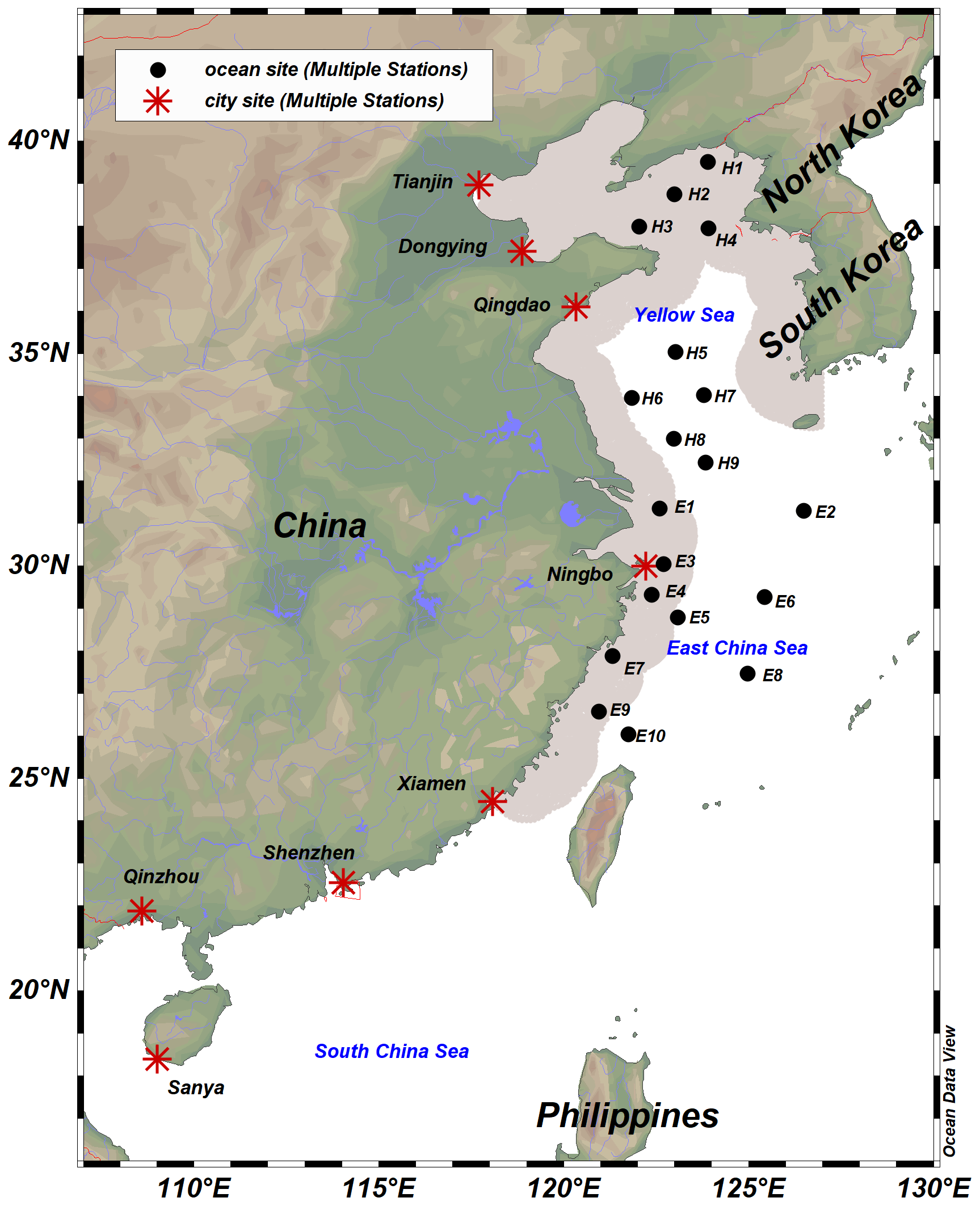
Figure 1 Map showing the sampling stations in the coastal cities (red asterisks) and marginal seas (black dots) of China from March to May 2021. The gray-shaded area represents the inshore region within 100 km from the coastline (Schlitzer, 2023).

2.2 Analysis of air samples

For the measurement of most types of gases, air samples were processed immediately after being brought back to the laboratory, using an atmospheric pre-concentrator system (8900DS, Nutech) coupled with a gas chromatograph–mass selective detector (GC-MSD) system (GC-7890A, MSD-5975, Agilent). The pretreatments of air samples were as follows. First, the atmospheric pre-concentrator system was baked for 10 min to clean the interior instrument. Then, trap 1 was cooled to −170 °C using liquid N₂, and a 300 mL air sample was pumped from the canister into trap 1 for the initial concentration of the target compounds, while N₂ and O₂ escaped due to their lower boiling points. After trap 2 was cooled to −50 °C, trap 1 was heated to 30 °C to transfer the target compounds from trap 1 to trap 2. Moisture and CO₂ were removed in the second concentration. Then, trap 2 was warmed up to transfer the target compounds into the last trap for cryofocusing (−175 °C). Finally, the last trap was instantaneously heated to 200 °C via gas bath heating, and the target compounds were delivered into the GC-MSD system by ultra-pure He.

For the parameter settings of GC-MSD, the temperature of the inlet, quadrupole, and ionization source was 150, 150, and 230 °C, respectively. The inlet was set to split mode with a ratio of 10:1. The flow rate of the carrier gas (He) was set to 1.5 mL min⁻¹ in the instant-flow mode. Specific columns were selected to separate the NMHCs (Rt-Alumina BOND/KCl, Restek), monocyclic aromatics (DB-624, Agilent), DMS (CP7529, Agilent), and VHCs (DB-624, Agilent). Gas standards of NMHCs in N₂ (Linde Gas, Germany) were diluted to 0.1–1 ppb for identification and calibration. Details of temperature programming and detector parameters can be seen in Zou et al. (2021) and Li et al. (2019). The precision and detection limits for the trace gases in the present study were 1 %–7 % and 0.03–20.0 ppt, respectively (Table S1 in the Supplement). Specifically, carbon monoxide (CO) was analyzed on site using a trace gas analyzer (TA3000R, Ametek) with a lower detection limit of 10 ppb; more details can be found in Xu et al. (2023). Note that data on DMS, CO, and VHCs from marine atmospheric samples were graciously provided by colleagues in the same laboratory. These data were used only as supporting information in the interpretation of our core dataset in this paper (e.g., correlation analysis).

2.3 Analysis of seawater samples

C2–C5 NMHCs in seawater were measured immediately on board using a purge and trap system coupled with the gas chromatography equipped with a flame ionization detector (GC-FID; 7890B, Agilent). The purge and trap system was improved based on a previously self-designed device described by Li et al. (2019). Briefly, seawater was collected using a customized glass sampler (500 mL) and connected to the inlet of the system. Then, seawater was transformed into the extraction cell under the pressure of pure N₂ and purged with pure-N₂ bubble flow (250 mL min⁻¹). The moisture of the carrier gas condensed in a thin glass tube that was placed in a cold chamber (4–6°), and the carbon dioxide was absorbed by a glass tube filled with Ascarite II (Merck). The targets were concentrated in a passivated stainless-steel tube immersed in liquid nitrogen for 26 min. Then, the steel tube was heated by boiling water, and the six-way valve was turned immediately for the inlet situation. The concentrated target compounds were transferred into the Rt-Alumina BOND/KCl capillary column for separation and were determined by FID. The parameters of the inlet, oven, and detector are shown in Table S2. The gas standard (Linde Gas, Germany) was diluted with ultra-pure N₂ to 10 ppb for identification and quantification. The instrumental blank was made to guarantee data reliability. The precision and detection limits were 3 %–6 % and 0.5–1.0 pmol L⁻¹ (Table S3).

2.4 Calculation of sea-to-air flux

The sea-to-air flux of each NMHC (F, nmol m⁻² d⁻¹) was calculated using Eq. (1):

$$\begin{array}{}\text{(1)}& F=k\times \left(C_{\mathrm{w}}-C_{\mathrm{a}}\times H\right),\end{array}$$

where k (m s⁻¹) is the gas transfer velocity described by Eq. (2); H is Henry's law constant; and C_w (pmol L⁻¹) and C_a (ppb) are concentrations of each NMHC in the surface seawater (5 m depth) and atmosphere, respectively.

$$\begin{array}{}\text{(2)}& k=\mathrm{0.31}\times u^{\mathrm{2}}\times {\left({\displaystyle \frac{Sc}{\mathrm{660}}}\right)}^{-\mathrm{0.5}}\end{array}$$

Here, u (m s⁻¹) is the wind velocity at 10 m. Sc is the Schmidt number, defined as Sc $=v/D$, and v is the kinematic viscosity of seawater calculated by Eq. (3) (Wanninkhof, 1992). D is the gas diffusion coefficient related to temperature and described by Eq. (4) (Wilke and Chang, 1955).

$$\begin{array}{}\text{(3)}& \begin{array}{rl}v& =\mathrm{1.052}+\mathrm{1.300}\times {\mathrm{10}}^{-\mathrm{3}}\times t+\mathrm{5.000}\times {\mathrm{10}}^{-\mathrm{6}}\times t^{\mathrm{2}}\\ & +\mathrm{5.000}\times {\mathrm{10}}^{-\mathrm{7}}\times t^{\mathrm{3}}\end{array}\end{array}$$

$$\begin{array}{}\text{(4)}& D={\displaystyle \frac{\mathrm{7.4}\times {\mathrm{10}}^{-\mathrm{8}}{\left(q\times M_{\mathrm{b}}\right)}^{\mathrm{0.5}}\times T}{n_{\mathrm{b}}\times V_{\mathrm{a}}^{\mathrm{0.6}}}}\end{array}$$

Here, t (°) is the degree Celsius of seawater, q is the association factor of water, M_b (g mol⁻¹) is the molar weight of water, T (K) is the degree Kelvin of seawater, n_b is the dynamic viscosity of seawater, and V_a is the molar volume at the boiling point.

2.5 Calculation of OFP and P_SOAP of NMHCs

To assess the environmental implications of NMHCs, the ozone formation potential (OFP; µg m⁻³) and secondary organic aerosol (SOA) formation potential (P_SOAP; µg m⁻³) are calculated using Eqs. (5) and (6), respectively (Carter, 1994):

$$\begin{array}{}\text{(5)}& {\displaystyle }{\mathrm{OFP}}_i={\mathrm{MIR}}_i\times C_i,\text{(6)}& {\displaystyle }{P}_{\mathrm{SOAPi}}=\sum C_i\times {\mathrm{SOAP}}_i\times {\mathrm{FAC}}_{\mathrm{toluene}}/\mathrm{100},\end{array}$$

where C_i represents the concentration of NMHCs; MIR_i (g O₃/g VOCs) and SOAP_i (relative to toluene = 100) are constants that represent the maximum incremental reactivity and SOA potential of i, respectively (Carter, 2010); and FAC_toluene is the fractional aerosol coefficient of toluene, which has a value of 5.4 % (Grosjean and Seinfeld, 1989). Specific data are listed in Table S11.

2.6 Normalized concentrations and lifetime-weighted concentrations of NMHCs

To effectively compare the NMHC variation with respect to the distance from the sampling sites to land (see Fig. 2d, f), we calculated the normalized concentration for each NMHC (C_Nor−i) using Eq. (7):

$$\begin{array}{}\text{(7)}& C_{\mathrm{Nor}\text{-}i}={\displaystyle \frac{C_i}{C_{\max \text{-}i}}},\end{array}$$

where C_i is the concentration of gas i, and C_max-i is the maximum of gas i.

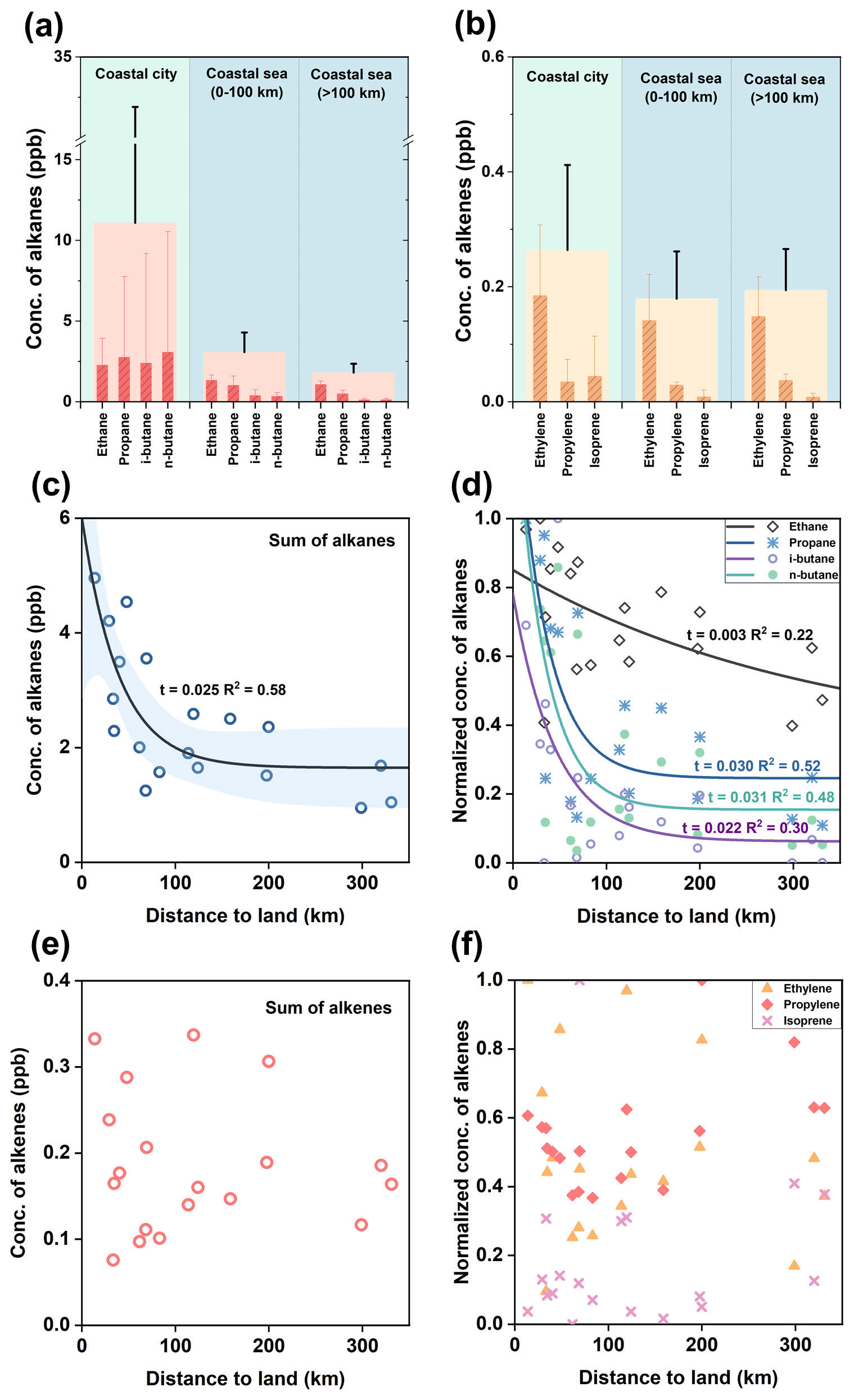
Figure 2 Means of the concentrations of alkanes (a) and alkenes (b) in the atmosphere over coastal cities (n=14) as well as nearshore (0–100 km, n=10) and offshore (> 100 km, n=9) coastal seas of China. The wider columns in panels (a) and (b) represent the sums of individual alkanes and alkenes, respectively, with error bars depicting the propagated errors from each NMHC. Summed alkane (c) and alkene (e) and normalized concentrations of specific alkane (d) and alkene (f) plotted as a function ($y=A{e}^{-tx}+y_{\mathrm{0}}$) of the distance from the sampling sites to the nearest land.

A novel approach was employed to analyze the correlation between the concentrations of various NMHCs and their sea-to-air fluxes. Concentrations were weighted according to the respective atmospheric •OH lifetime of each NMHC. This was achieved by dividing the concentration of each NMHC by its corresponding atmospheric •OH lifetime, yielding a “lifetime-weighted concentration” for each NMHC (C_life−i) (Eq. 8). This method provides a more nuanced understanding of the impact of oceanic emissions on NMHCs, taking into account not only their abundance but also their residence in the atmosphere.

$$\begin{array}{}\text{(8)}& C_{\mathrm{life}\text{-}i}={\displaystyle \frac{C_i}{{\mathit{\tau }}_i}}\end{array}$$

Here, C_i is the atmospheric concentration of gas i, and τ_i is the •OH lifetime of gas i. The approximate atmospheric lifetime of each NMHC was calculated assuming an average [•OH] of 6×10⁵ molec. cm⁻³ within 24 h at 288 K (Jobson et al., 1999), with specific data listed in Table 1.

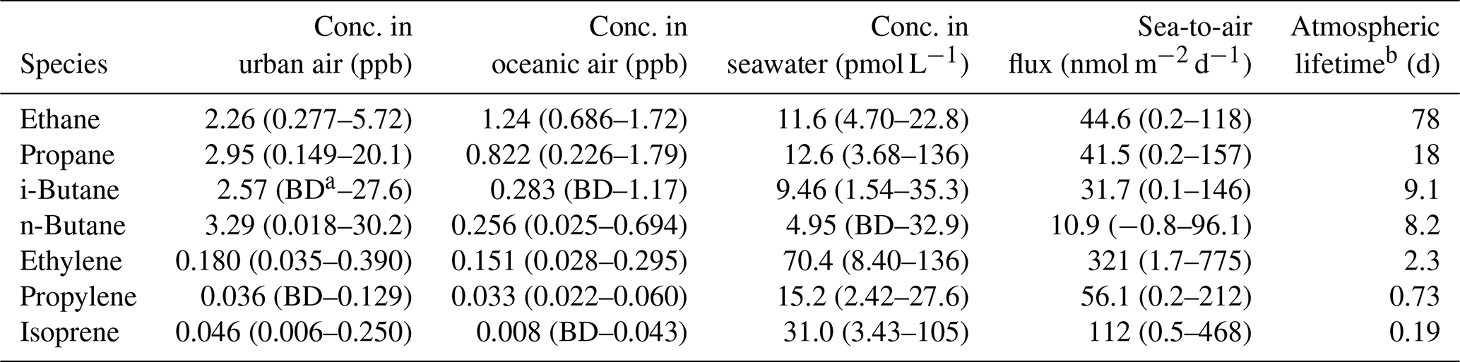
Table 1 Atmospheric and seawater concentrations, sea-to-air fluxes, and the calculated atmospheric lifetime of each NMHC based on the reaction with hydroxyl radicals (•OH).

^a Below the detection limit. ^b Assuming an average [•OH] of 6×10⁵ molec. cm⁻³ within 24 h (Jobson et al., 1999) and using the rate constant with •OH at 288 K taken from Atkinson et al. (1997).

2.7 Calculation of the shortest distance from the sampling station to land

Coastline latitude and longitude data near the study area (20–45° N, 110–130° E) were extracted from the World Vector Shoreline (Wessel and Smith, 1996). Subsequently, distances from the maritime sampling stations to all coastal locations were computed. The minimum value among these distances was selected as the shortest distance to land (listed in Table S9).

2.8 Calculation of retention of air mass over land

To identify whether an air mass was mainly from terrestrial or oceanic regions, the retention ratio of the air mass over land (R_L) was calculated by Eq. (9):

$$\begin{array}{}\text{(9)}& R_{\mathrm{L}}={\displaystyle \frac{{\sum }_{n=\mathrm{1}}^{N_{\mathrm{land}}}{e}^{-\frac{t_n}{\mathrm{48}}}}{{\sum }_{n=\mathrm{1}}^{N_{\mathrm{total}}}{e}^{-\frac{t_n}{\mathrm{48}}}}},\end{array}$$

where N_total is the total number of trajectory endpoints (Stein et al., 2015). N_land is the total number of trajectory endpoints located over land, while t_n is the backward tracking time in units of hours, and $e^{-\frac{t_n}{\mathrm{48}}}$ is the weighting factor related to tracking time as the diffusion of air mass takes place along the transport path rather than in the nearby regions. As a result, the larger R_L value indicates that the air mass is more influenced by terrestrial transport, and its source is more likely to be on land. Similar methods have been used to calculate the average residence time of sampled air masses in the Arctic (Willis et al., 2017) and identify the percentage of time spent by trajectories over different surface types in the Antarctic (Decesari et al., 2020). R_L values were calculated by three different timescale trajectories (48, 72, and 96 h) (listed in Table S9). The mean R_L (n=3) was finally applied to analyze the terrestrial influence on oceanic NMHCs, mitigating the uncertainty caused by the trajectory with different timescales.

2.9 Application of the PMF model

The PMF model, introduced in detail in the study of Paatero and Tapper (1994), was applied to analyze the data of atmospheric NMHCs in the Yellow Sea and the East China Sea. Based on a matrix consisting of the concentrations of diverse chemical species, the objective of PMF is to determine the number of NMHC source factors, the chemical composition profile of each factor, and the contribution of each factor to species. The matrix representation of this model is (Eq. 10)

$$\begin{array}{}\text{(10)}& x_{ij}=\sum _{k=\mathrm{1}}^p{g}_{ik}{f}_{kj}+e_{ij},\end{array}$$

where x_ij represents the concentration of species j measured on sample i, and p denotes the number of factors facilitating the samples. f_kj represents the concentration of species j in factor profile k, g_ik denotes the relative contribution of factor k to sample i, and e_ij represents the PMF model error of species j measured on sample i. The factors resolved by PMF are typically interpreted as sources. The objective of this algorithm is to find the values of f_kj, g_ik, and p that best reproduce x_ij, continuously adjusting f_kj and g_ik until the minimum Q value for a given p is attained. Q is defined as Eq. (11):

$$\begin{array}{}\text{(11)}& Q=\sum _{i=\mathrm{1}}^n\sum _{j=\mathrm{1}}^m{\left({\displaystyle \frac{e_{ij}}{{\mathit{\sigma }}_{ij}}}\right)}^{\mathrm{2}},\end{array}$$

where σ_ij represents the uncertainty in the concentration of species j in sample i, n is the number of samples, and m is the number of species. In applying the PMF model, the significance of missing data in the matrix was decreased by using the species median. The uncertainty for normal data was estimated as 20 % of the NMHC concentrations because the analytical uncertainty was not available (Buzcu and Fraser, 2006). The model was run 20 times, and we selected the result with the minimum Q value. Additionally, scaled residuals are instrumental in assessing the fit of the PMF model to the observed data. They represent the difference between the observed and modeled data, scaled by the uncertainty in the observed data. In this PMF analysis, approximately 94 % of the scaled residuals ranged from −3 to 3 (Fig. S1), suggesting a reasonable fit of the model result.

3 Results and discussion

3.1 Atmospheric concentrations of NMHCs in coastal cities and marginal seas of China

To clarify, NMHCs determined in this study were separated into two groups for further discussion based on their distinctly different atmospheric reactivity and lifetimes: alkanes (long lifetime, 8.2–78 d) and alkenes (short lifetime, 0.19–2.3 d). In the urban atmosphere (n=14), the mean (range) concentration of ethane, propane, i-butane, and n-butane was 2.26±1.66 (0.277–5.72), 2.95 ± 5.12 (0.149–20.1), 2.57 ± 6.99 (BD–27.6), and 3.29 ± 7.68 (0.018–30.2) ppb, respectively (Table 1). Alkanes combined accounted for ∼ 76 %–99 % of total NMHCs measured in this study, which agrees with previous studies reporting alkanes as the dominant NMHCs in the urban atmosphere of China, e.g., 43.7 % (Song et al., 2007) and > 50 % (Li et al., 2015). For alkene species in the urban atmosphere (n=14), the mean (range) of ethylene, propylene, and isoprene was 0.180 ± 0.126 (0.035–0.390), 0.036 ± 0.040 (BD–0.129), and 0.046 ± 0.072 (0.006–0.250) ppb, respectively.

Similarly, alkanes were also dominant components in the marine atmosphere, accounting for ∼ 86 %–95 % of NMHCs. In the marine atmosphere (n=19), the mean (range) concentration of ethane, propane, i-butane, n-butane, ethylene, propylene, and isoprene was 1.24 ± 0.298 (0.686–1.72), 0.822 ± 0.518 (0.226–1.79), 0.283 ± 0.302 (BD–1.17), 0.256 ± 0.214 (0.025–0.694), 0.151 ± 0.077 (0.028–0.295), 0.033 ± 0.009 (0.022–0.060), and 0.008 ± 0.010 (BD–0.043) ppb, respectively. These values were comparable to those reported in the Bay of Bengal (Sahu et al., 2011) and the northwestern Pacific Ocean (Li et al., 2019) (Table S6). Alkanes in the urban atmosphere were on average more than 4 times higher than those in the marine atmosphere, while no significant difference was observed for concentrations of alkenes between urban and marine air (t=2.224, p=0.156) (Fig. 2a, b). In spatial terms, multiple NMHCs (e.g. ethane, propane, i-butane, n-butane, and ethylene) showed higher atmospheric concentrations in regions closer to land. The elevated concentrations were primarily concentrated along the coastal regions of the East China Sea and the north Yellow Sea (Fig. S3). The disparity in NMHC concentrations between land and ocean, as well as the distribution pattern of NMHCs in the marine atmosphere, suggested a potential influence of terrestrial sources on the oceanic NMHCs.

3.2 Atmospheric NMHC variability vs. estimated lifetime

The standard deviation of the natural logarithm of the NMHC mixing ratios (S_lnx) was established to correlate to their •OH lifetime (τ) in the atmosphere following an exponential function of $S_{\ln x}=A{\mathit{\tau }}^{-b}$ (Jobson et al., 1998), where A and b are fitting parameters. A b value approaching 0 suggests that the NMHC variability is primarily controlled by local emission fluctuations, while a b value of 1 indicates the minimal impact of local emissions, with the variability predominantly controlled by the extent of photochemical reactions.

Employing the analytical framework in Jobson et al. (1998), we analyzed our atmospheric NMHC data from urban areas and the Chinese marginal seas. The derived b value for urban areas was 0.05 (Fig. 3a), suggesting that atmospheric NMHCs in coastal cities were mainly controlled by local emissions. In the marine atmosphere, the b value was 0.26 (Fig. 3b), which was comparable to values reported for Gosan (0.30) (Wong et al., 2007) and continental outflow from southern China (0.31) (Wang et al., 2005), but it was significantly lower than the values for Ogasawara (0.43) (Kato et al., 2004), the northwestern Indian Ocean (0.40) (Warneke and de Gouw, 2001), and the South China Sea (0.42) (Wang et al., 2005). The b value of 0.26 in the atmosphere over the Chinese marginal seas suggests that the NMHC composition in the nearshore atmosphere is influenced by both the local oceanic emissions and the remote sources from the continent. As sites closer to the source position tend to have lower b values, the Yellow Sea and the East China Sea experience a more pronounced influence from terrestrial pollution sources compared to Ogasawara, the South China Sea, and the northwestern Indian Ocean.

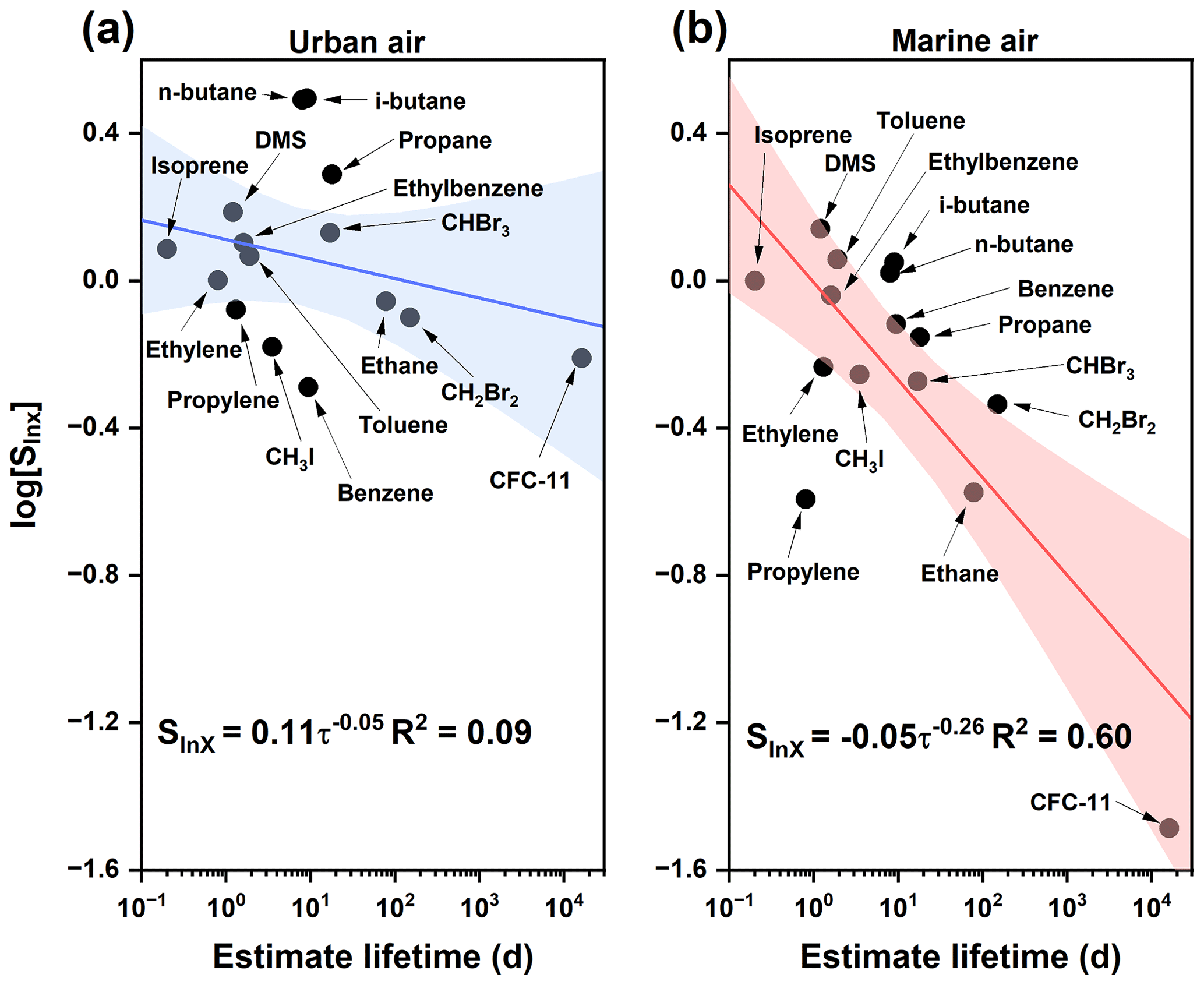
Figure 3 Atmospheric variability (log[S_lnx]) plotted as a function of the estimated •OH lifetime for each NMHC from the coastal cities (a) and marginal seas of China (b). The blue and red lines are the best linear fit. The shadowed area represents the confidence band at a 95 % confidence level.

3.3 Terrestrial influence on marine atmospheric NMHC variation

Given the discernible impact of terrestrial input on the spatial distributions and variabilities of marine atmospheric NMHCs, we further elucidated the role of terrestrial outflow in shaping marine atmospheric NMHC levels. This examination focused on three key factors: distance from the sampling site to land, retention of air mass over land, and transport time of air mass.

3.3.1 Distance from the sampling site to land

The distances from the oceanic sampling sites to the nearest land spanned 13.9 to 331 km, with an average of 123 km (Table S9). Significant correlations were observed between the distances and concentrations of ethane ($r=-\mathrm{0.553}$, n=19, p=0.014), propane ($r=-\mathrm{0.605}$, n=19, p=0.006), i-butane ($r=-\mathrm{0.513}$, n=19, p=0.025), and n-butane ($r=-\mathrm{0.573}$, n=19, p=0.010). When plotted against the distances, the concentrations of alkanes combined decreased with increasing distance (Fig. 2c), and different species exhibited distinctly specific decreasing rates (Fig. 2d). Since the concentrations between different NMHC species varied considerably, the normalized concentrations were employed to fit an attenuation equation ($y=A{e}^{-tx}+y_{\mathrm{0}}$) for each species. As shown in Fig. 2d, the attenuation coefficients for ethane, propane, i-butane, and n-butane are 0.003, 0.030, 0.031, and 0.022, respectively. These coefficients were correlated with their atmospheric reactivities. Species with lower reactivity and longer lifetimes, such as ethane (with a lifetime of 78 d), have the lowest attenuation coefficient. This implies that long-lifetime species could be affected by the terrestrial input even at a more remote marine site. Terrestrial influences on propane, i-butane, and n-butane were discernible only in areas much closer to land, as their concentrations stabilized at low values beyond a distance of around 100 km (Fig. 2d).

3.3.2 Retention of air mass over land

A larger retention of air mass over land (R_L) has previously been suggested to serve as an indicator of a greater terrestrial influence (Zhou et al., 2021). To mitigate the uncertainty derived from varying timescale trajectories, we calculated R_L−mean based on 48, 72, and 96 h backward trajectories. R_L−mean ranged from 0.10 to 0.96 (Table S9). When plotted against R_L−mean, a linear relationship was observed between the concentrations of NMHCs combined and R_L−mean, with a slope of 2.51 (Fig. 4a). A statistically significant correlation (r=0.599, n=19, p=0.007) was observed when only plotting alkanes with R_L−mean. However, the correlation between alkenes and R_L−mean was statistically insignificant (r=0.248, n=19, p=0.306).

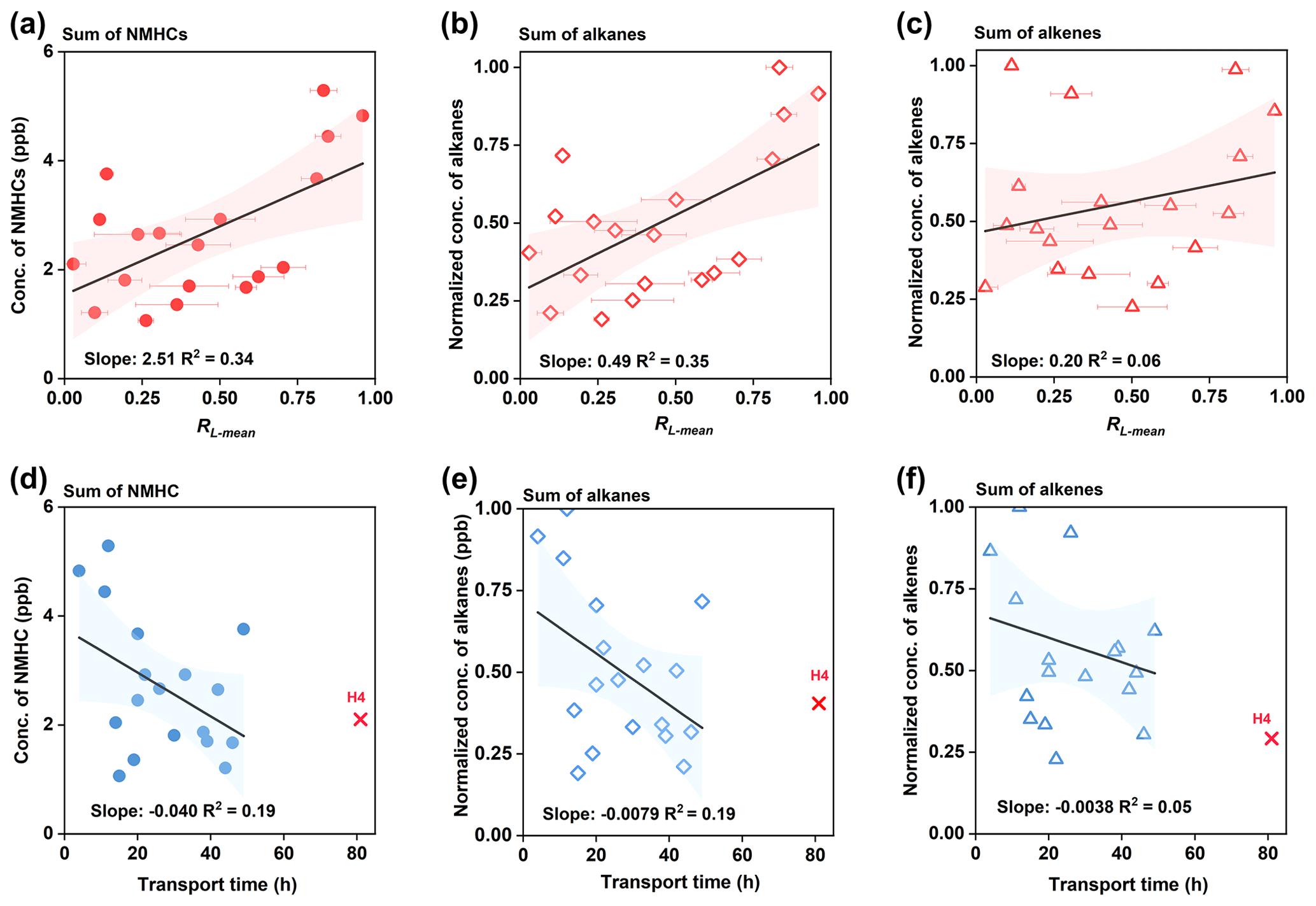
Figure 4 Concentrations of NMHCs combined (a, d), alkanes (b, e), and alkenes (c, f) at each site plotted against the mean retentions of air mass over land (R_L−mean, n=3) and the transport time of air mass, respectively. The error bars for R_L−mean indicate the standard deviation from three different timescale trajectories (48, 72, and 96 h). The black line is the best fit of the liner function, and the shadowed area represents the confidence band at a 95 % confidence level. H4 (marked with red “×”) is treated as an outlier since it is the only value that deviates from the main dataset.

3.3.3 Transport time of air mass

The transport time of air mass was estimated as the interval from the last point of the trajectory contacting the continent to the moment when the air mass reached the sampling location, as detailed by Kato et al. (2001). These times ranged from 4 to 81 h, with an average of 30 h (Table S9). A shorter air mass transport time signifies a stronger terrestrial influence, as NMHCs within the air mass undergo further oxidation and dispersion over time. Total NMHC concentrations exhibited a significant decrease with an increase in air mass transport time, characterized by a slope of −0.04 (Fig. 4d). Alkanes displayed a steeper decline, indicated by a slope of −0.0079 (Fig. 4e), compared to alkenes (−0.0038, Fig. 4f). Notably, elevated alkane concentrations were affected by air masses with larger R_L−mean (> 0.8) and shorter transport time (< 20 h) (Fig. S4). This emphasized the terrestrial influence on alkanes in the marine atmosphere since both R_L and transport time serve as indicators of air mass terrestrial characteristics. However, similar to the analysis of R_L, the correlation between the air mass transport time and alkenes was statistically insignificant (r=0.248, n=19, p=0.306).

Overall, the analysis above suggests that the terrestrial input plays an important role in driving the variability observed for the atmospheric NMHCs over the marginal seas of China. In particular, a stronger terrestrial impact was determined for the alkanes based on the larger slopes from linear regression analysis and the significant correlations with terrestrial indicators. In contrast, no discernible trend was found for alkenes when plotting their concentrations against the distance from sampling sites to the coastline (Fig. 2e, f). There was no significant correlation between alkenes and R_L or air mass transport time. Therefore, the variability of alkenes in the coastal atmosphere seems to be weakly impacted by the terrestrial sources when compared to alkanes. We attribute this to two main factors. First, the mean concentration of alkenes in the urban air was only 1.4 times higher than in the marine air, whereas it was 5.4 times higher for alkanes. Alkenes undergo more rapid oxidation due to their higher reactivities compared to alkanes during air mass transport. Secondly, oceanic ventilation may play a more substantial role in affecting marine alkenes (discussed in Sect. 3.4).

3.4 Oceanic impact on marine atmospheric NMHC composition

3.4.1 Sea-to-air fluxes of NMHCs

The mean (range) of sea-to-air fluxes of ethane, propane, i-butane, n-butane, ethylene, propylene, and isoprene was 44.6 ± 35.0 (0.2–118), 41.5 ± 39.9 (0.2–157), 31.7 ± 38.2 (0.1–146), 10.9 ± 25.4 (−0.8–96.1), 321 ± 294 (1.7–775), 56.1 ± 55.2 (0.2–212), and 112±134 (0.5–468) nmol m⁻² d⁻¹, respectively, in the Yellow Sea and the East China Sea (Table 1). These values were comparable to those reported in Chinese marginal seas (Wu et al., 2021; Li et al., 2021) and the 23–38° N Atlantic Ocean (Tran et al., 2013), but they were larger than the reported values in the North Sea (Broadgate et al., 1997) and the northwestern Pacific Ocean (Li et al., 2019; Wu et al., 2023) (Table S10).

The averaged sea-to-air fluxes of alkanes and alkenes within 100 km from the coastline were 147 ± 116 and 551 ± 497 nmol m⁻² d⁻¹, respectively, which were relatively higher than those beyond 100 km (Fig. 5a, b). Since there were no significant differences in surface seawater temperature and 10 m wind speed between regions within and beyond 100 km from the coastline (Fig. S5), the discrepancy in fluxes might not be driven by physical processes. These elevated fluxes in the sea areas closer to land could be attributed to the influence of phytoplankton biomass and chromophoric dissolved organic matter (CDOM). Seawater NMHCs are not only directly synthesized by phytoplankton (Ratte et al., 1995), but they can also be emitted through the photochemical degradation of CDOM (Ratte et al., 1993; Lee and Baker, 1992). To substantiate our findings, we analyzed the monthly Chl-a concentration and the absorption coefficient at 443 nm of seawater in April 2021 from the remote sensing dataset from the NASA Ocean Color data service (NASA Ocean Biology Processing Group, 2022a, b) (Fig. S2). The mean (± SD) of Chl-a concentrations was 2.83±1.17 and 1.68±1.44 µg L⁻¹ in the areas within and beyond 100 km from the coastline, respectively. Correspondingly, the mean (± SD) of seawater absorption coefficients at 443 nm was 0.124±0.060 and 0.069±0.040 m⁻¹, respectively. Hence, the heightened phytoplankton biomass and enriched photoreaction substrate collectively enhanced both the biological production of NMHCs and the abiotic formation of NMHCs, consequently resulting in a pronounced NMHC emission in nearshore regions.

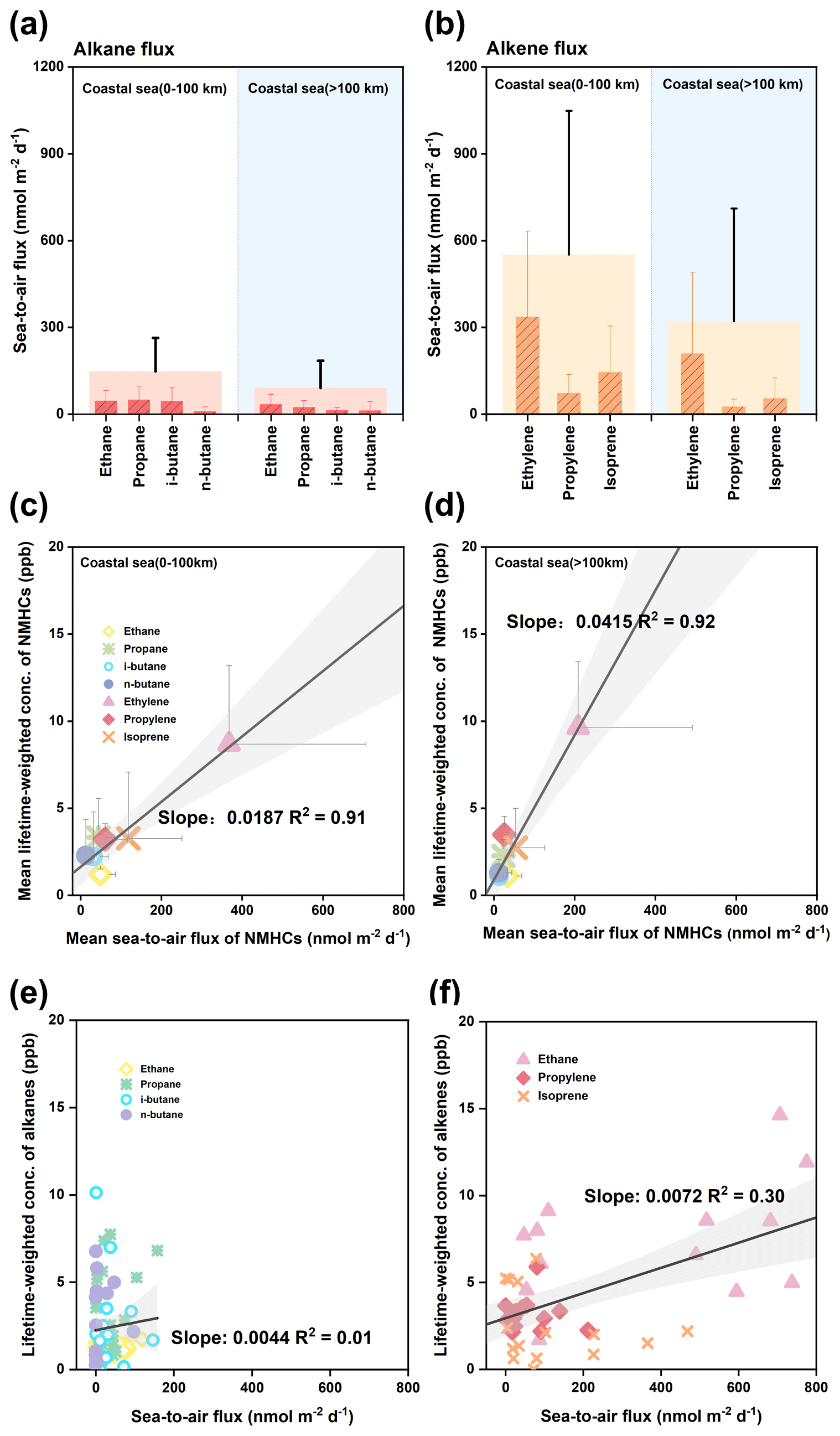
Figure 5 Means of sea-to-air fluxes of alkanes (a) and alkenes (b) in sea areas within 100 km (n=10) and beyond 100 km (n=9) from the nearshore land. The wider columns represent the sum of alkanes and alkenes. Panels (c) and (d) show the means of lifetime-weighted concentrations of NMHCs plotted against their mean sea-to-air fluxes in the area within 100 km or beyond 100 km from the coastline. Specific lifetime-weighted concentrations of alkanes (e) and alkenes (f) plotted against sea-to-air fluxes in the whole coastal sea region. The black lines are the best linear fit for each dataset, and the shadowed area represents the confidence band at a 95 % confidence level.

3.4.2 Assessing the effect of oceanic emission on NMHCs

Prior to delving into the correlation between oceanic emissions and NMHC concentrations, it is imperative to acknowledge the influence of different gases' reactivity on this relationship. For instance, ethane possesses an atmospheric lifetime of approximately 78 d at 24 h [•OH] concentration of 6×10⁵ molec. cm⁻³ (Jobson et al., 1999), using the rate constant with •OH at 288 K taken from Atkinson et al. (1997). The relatively long atmospheric residence time of ethane facilitates its accumulation in the atmosphere. Conversely, isoprene, with a much shorter lifetime of only 0.2 d, emitted within a very brief window can impact its atmospheric level. Thus, to mitigate the impact of varying reactivity among the different gas species, we calculated the lifetime-weighted concentrations of each NMHC according to its atmospheric lifetime (introduced in Sect. 2.5). This novel method is more nuanced in assessing the impact of oceanic emission on atmospheric NMHCs, as it acknowledges not only their abundance but also their residence in the atmosphere.

Despite the elevated oceanic emission of NMHCs within 100 km from land, its impact on atmospheric NMHC composition was comparatively weak, displaying a slope of 0.0187 (Fig. 5c), which was lower than the fitted result of the dataset in areas beyond 100 km from land with a slope of 0.0415 (Fig. 5d). This could be attributed to the disturbance of terrestrial outflow in nearshore areas, mitigating the direct impact of oceanic emission on NMHCs. As it extended further from land, the terrestrial influence diminished. This, in turn, strengthens the regulatory impact of oceanic emission on atmospheric NMHC levels.

In addition, the average flux of total alkenes across the entire region was 163 ± 221 nmol m⁻² d⁻¹, which was approximately 5 times higher than that of alkanes (32.2 ± 37.5 nmol m⁻² d⁻¹). This substantial discrepancy indicates that alkanes and alkenes are certainly influenced differently by oceanic emissions. The correlation between the lifetime-weighted concentrations of alkenes and their fluxes was statistically significant (r=0.548, n=57, p<0.001), while it was insignificant for alkanes (r=0.113, n=76, p=0.329). When specific species of alkanes (Fig. 5e) and alkenes (Fig. 5f) were separately plotted against their sea-to-air fluxes, alkenes exhibited a steeper slope of 0.0072 compared to the slope of 0.0044 for alkanes. This signifies that oceanic emission has a more significant impact on atmospheric alkenes compared to alkanes, which verifies our hypothesis as stated at the end of Sect. 3.3.

3.5 Identification and apportionment of the sources of marine atmospheric NMHCs

3.5.1 Source identification

Since the chemical compositions are largely controlled by the sources of emissions, specific ratios of hydrocarbons have been widely employed to identify the sources of NMHCs (Gilman et al., 2013; Rossabi and Helmig, 2018). For instance, elevated isopentane$/$n-pentane ratios are indicative of the large influence of vehicular emissions (2.2–3.8) and gasoline fuel evaporation (1.8–4.6) (Gentner et al., 2009; Jobson et al., 2004; Liu et al., 2008; Russo et al., 2010). Conversely, the lower ratios indicate the importance of tropical forest fires (0.43–0.57) (Andreae and Merlet, 2001; Rossabi and Helmig, 2018), natural and oil gas operations (0.81–1.1) (Gilman et al., 2013; Swarthout et al., 2013), and marine vessel exhaust (1.59–1.71) (Bourtsoukidis et al., 2019) in controlling the chemical composition of NMHCs. In this study, a significant correlation was observed between i-pentane and n-pentane (r=0.67, p<0.01) (Fig. 6), and the i-pentane$/$n-pentane ratio spans a wider range from 0.89 to 2.46, suggesting that the composition of NMHCs in the marginal seas of China is controlled by multiple sources, e.g., natural and oil gas operations, marine vessel exhaust, vehicular emissions, and gasoline evaporation.

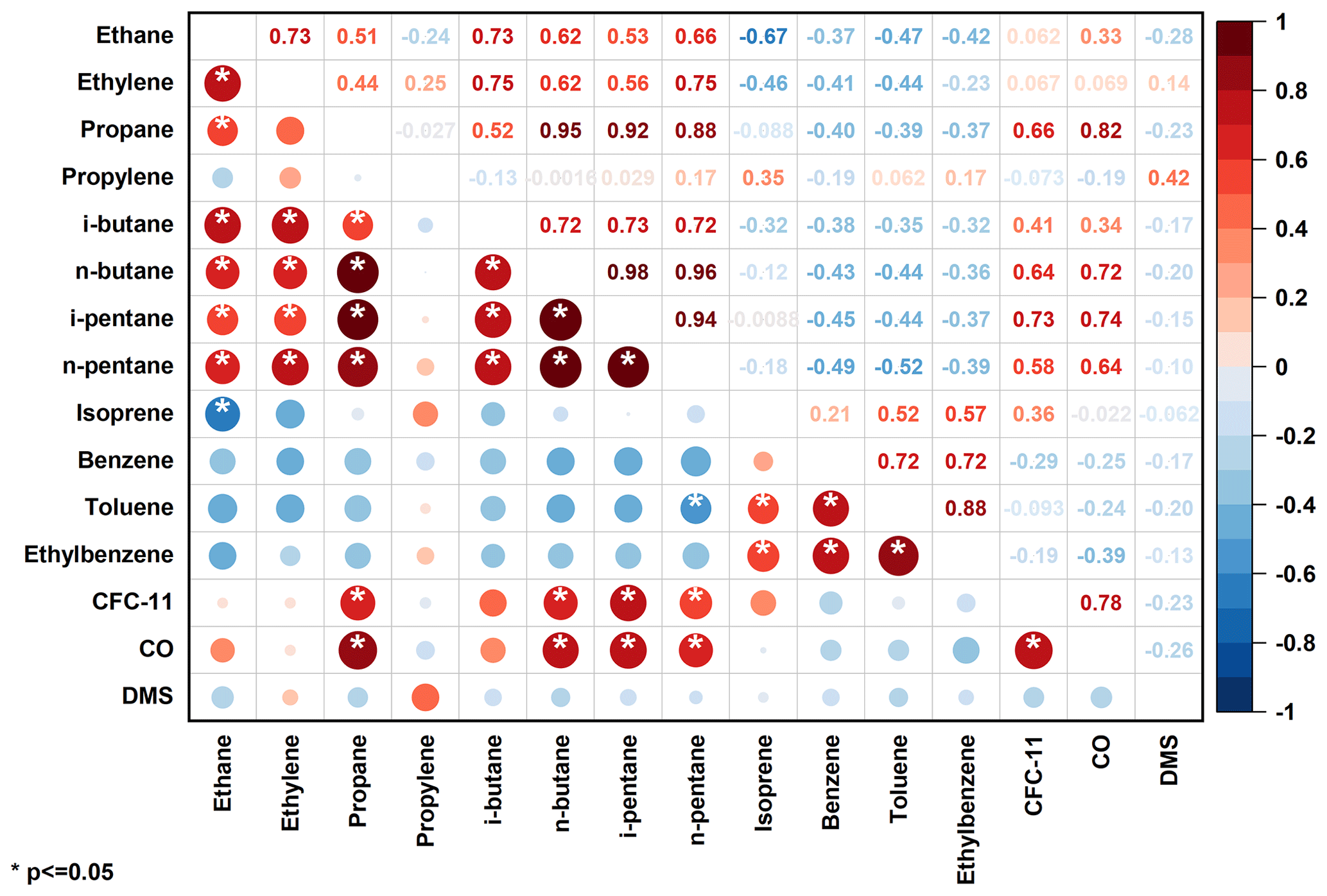
Figure 6 Correlation coefficients (r) between the various trace gases determined in the atmosphere over the Yellow Sea and the East China Sea. The white asterisk means the correlation is significant at p<0.05. The color of the dots, red and blue, indicates the positive and negative correlation, and the size of the dots indicates the absolute value of r.

Furthermore, propane, i-butane, and n-butane exhibited strong intercorrelations (r=0.52–0.95, p<0.05). They also displayed strong correlations with ethane, i-pentane, and n-pentane (r=0.55–0.98, p<0.05). These alkanes have been recognized as the primary components of liquid petroleum gases (Blake and Rowland, 1995), extensively utilized as fuel in taxis, private cars, and public buses in China (Guo et al., 2017; Zhang et al., 2015). Notably, C3–C5 alkanes also exhibited significant correlations with ethane (r=0.55–0.72, p<0.05) and carbon monoxide (r=0.59–0.81, p<0.05), while ethane and carbon monoxide are acknowledged tracers of fossil fuel or biomass/biofuel combustion and incomplete combustion, respectively (Lai et al., 2010; Tang et al., 2009; Parrish et al., 2009). This indicated the contribution of vehicular emissions of liquid petroleum gases and combustion of fossil fuel or biomass to light alkanes. Additionally, strong correlations were observed among monocyclic aromatics (benzene, toluene, ethylbenzene) (r=0.67–0.83, p<0.05). This finding was consistent with recent emission inventory research identifying monocyclic aromatics as significant constituents of ship exhaust (Xiao et al., 2018b; Wu et al., 2019). As for oceanic emissions, we present the sea-to-air fluxes of NMHCs and discuss the significant effect of oceanic emissions on NMHCs in Sect. 3.4. Multiple studies have highlighted that the ocean is one of the most important sources of these gases (Kato et al., 2007; Li et al., 2019; Mallik et al., 2013; Sahu et al., 2010; Rudolph and Johnen, 1990).

3.5.2 Source apportionment

The potential sources of atmospheric NMHCs and their respective contributions to each category were determined using the PMF model. Four isolate factors were extracted according to their composition profiles depicted in Fig. 7a. These factors, including industrial production, exhaust emission, terrestrial vegetation, and oceanic ventilation, were identified based on chemical profiles in the literature.

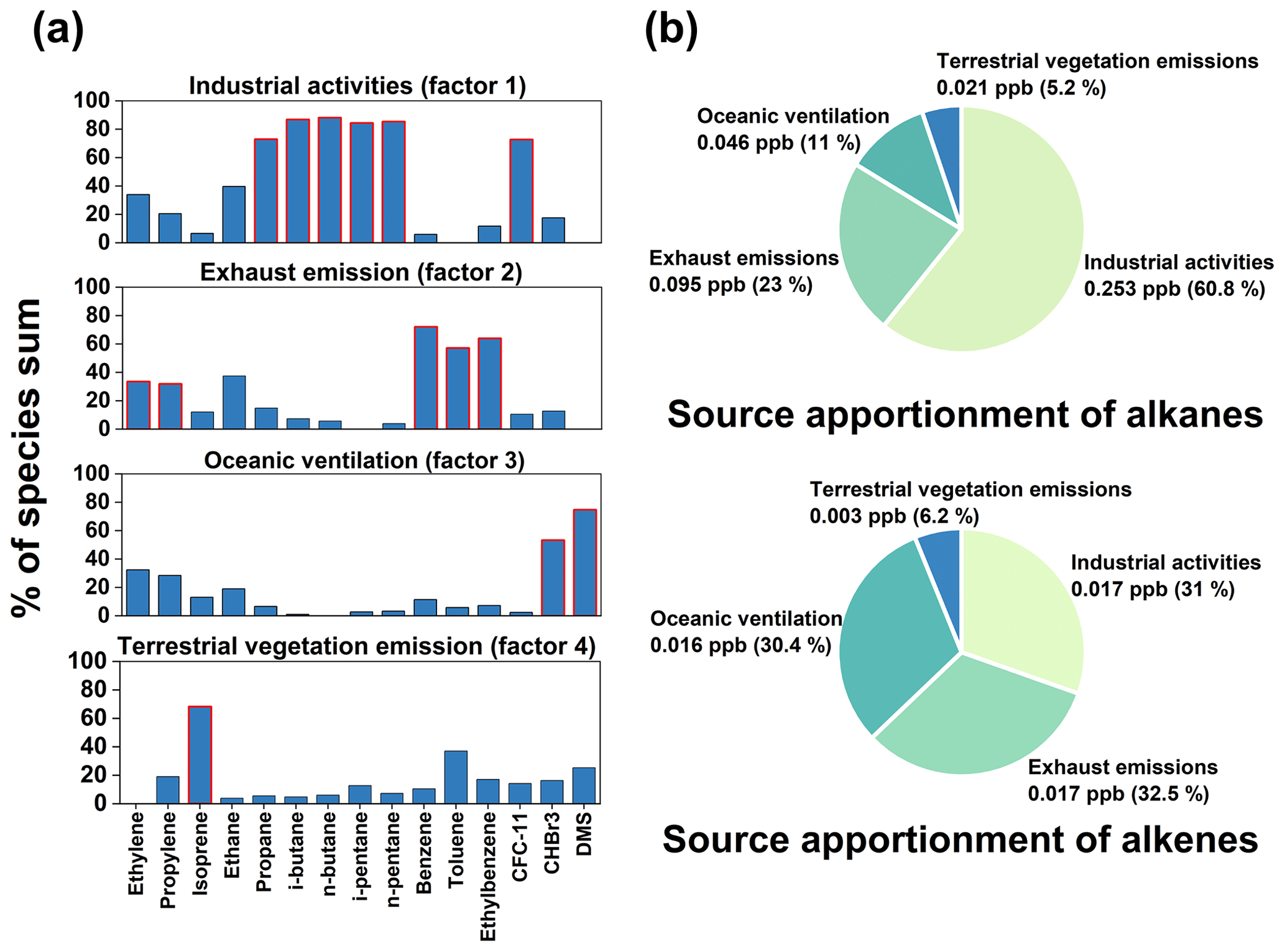
Figure 7 Representative factor profiles from the PMF model (a) and relative contributions of different factors/sources to the alkanes and alkenes in the oceanic atmosphere (b). NMHCs in panel a marked with red rim are selected as indicators for the specific factors.

Propane, i-butane, n-butane, i-pentane, n-pentane, and CFC-11 showed strong loadings (> 70 %) on factor 1. The presence of propane, butanes, and pentanes suggests an influence of refinery activities (Buzcu and Fraser, 2006). Additionally, propane has been recognized as a characteristic NMHC derived from natural gas emissions, and butane is indicative of liquefied petroleum gas (LPG) (Guo et al., 2011; Tsai et al., 2006; Hui et al., 2018; Ho et al., 2009). Moreover, CFC-11 is a typical artificial industrial product. Subsequently, factor 1 was identified as a factor relating to industrial activities.

The profile of factor 2 showed strong loadings of benzene (72 %), toluene (57 %), and ethylbenzene (64 %), along with moderate impacts of ethylene (34 %) and propylene (32 %). Benzene emissions are notably associated with vehicle exhaust (Zhang et al., 2013, 2016), and considerable fractions of aromatics can be emitted from ship exhaust during both berthing and cruising (Cooper, 2005; Xiao et al., 2018a). C2–C4 alkenes could stem from ship emissions in the open ocean (Eyring et al., 2005). Therefore, factor 2 can be assigned as a potential source of exhaust emissions of vehicles and ships.

Factor 3 was assigned as oceanic ventilation due to elevated percentages of DMS (74 %) and CHBr₃ (53 %), considering the dominant contributions of ocean emission to DMS (Lana et al., 2011; Lee and Brimblecombe, 2016) and CHBr₃ (Quack and Wallace, 2003; Ashfold et al., 2014). Factor 4 was mainly characterized by a high percentage of isoprene (68 %), an indicator of biogenic emission from terrestrial vegetation (Guenther et al., 2006; Wu et al., 2016). However, given isoprene's high reactivity, this factor should be treated cautiously and regarded as a lower limit (Fujita, 2001). Although its short atmospheric lifetime hinders long-range transport, the minimum air mass transport time from land to the oceanic station was 4 h in this study, implying the potential for terrestrial isoprene to reach the nearshore atmosphere.

According to the results of the PMF model analysis, the dominant source of atmospheric alkanes in the Chinese marginal seas was industrial activities (0.253 ppb, 60.8 %), followed by exhaust emissions (0.095 ppb, 23 %). Contributions from terrestrial vegetation emission (0.049 ppb, 11 %) and oceanic ventilation (0.021 ppb, 5.2 %) were relatively smaller. Furthermore, exhaust emissions (0.017 ppb, 32.5 %), industrial activities (0.017 ppb, 31 %), and ocean ventilation (0.016 ppb, 30.4 %) contribute almost equally to atmospheric alkenes. Collectively, these three factors constitute the main sources of alkenes (93.8 %), whereas the contribution from terrestrial vegetation is minimal, at merely 6.2 %. Particularly, the contribution of terrestrial sources to alkanes (89 %) is greater than that to alkenes (69.6 %), while the contribution of ocean emission to alkenes (30.4 %) is greater than that to alkanes (5.2 %). This is consistent with the conclusions in Sect. 3.3 and 3.4.

It must be acknowledged that the classification and quantification results derived from the PMF model inevitably involve uncertainties that are challenging to ascertain precisely. These uncertainties are primarily attributed to factors such as the number of gas species, the number of samples, and the temporal and spatial resolutions of sampling. However, it is noteworthy that the PMF analysis results are relatively consistent with the phenomena described in Sect. 3.3 and 3.4. This consistency to some extent validates the accuracy of the PMF analysis and underscores the significant contribution and impact of terrestrial inputs on the atmospheric NMHCs in the marginal seas of China.

3.5.3 Contributions of terrestrial/oceanic NMHCs to SOA and ozone

P_SOAP of the C2–C5 NMHCs in the atmosphere over the Chinese marginal seas was 0.41 ± 0.18 µg m⁻³, with terrestrial sources contributing the majority (0.32 ± 0.14 µg m⁻³), accounting for approximately 78 % (Fig. 8a). Specifically, P_SOAP from terrestrial alkanes and alkenes was 0.17 ± 0.07 and 0.15 ± 0.06 µg m⁻³, respectively, while marine sources contributed 0.02±0.01 and 0.07 ± 0.03 µg m⁻³ for alkanes and alkenes, respectively. Additionally, troposphere aerosol concentrations over the Chinese marginal seas during the investigation period were calculated using data from the NASA Goddard Earth Sciences Data and Information Services Center (GES DISC), ranging from 0.77 to 3.98 µg m⁻³, with an average of 1.80 ± 0.71 µg m⁻³. The aerosol concentrations decreased from the coastal areas towards the open sea (Fig. 8b), suggesting an obvious influence of terrestrial inputs on the aerosol levels in the coastal atmosphere. Based on the remote sensing data, it is roughly estimated that terrestrial C2–C5 NMHCs contribute ∼ 18 % to the total aerosol concentration, indicating their non-negligible role in influencing the atmospheric aerosol levels over the marginal seas.

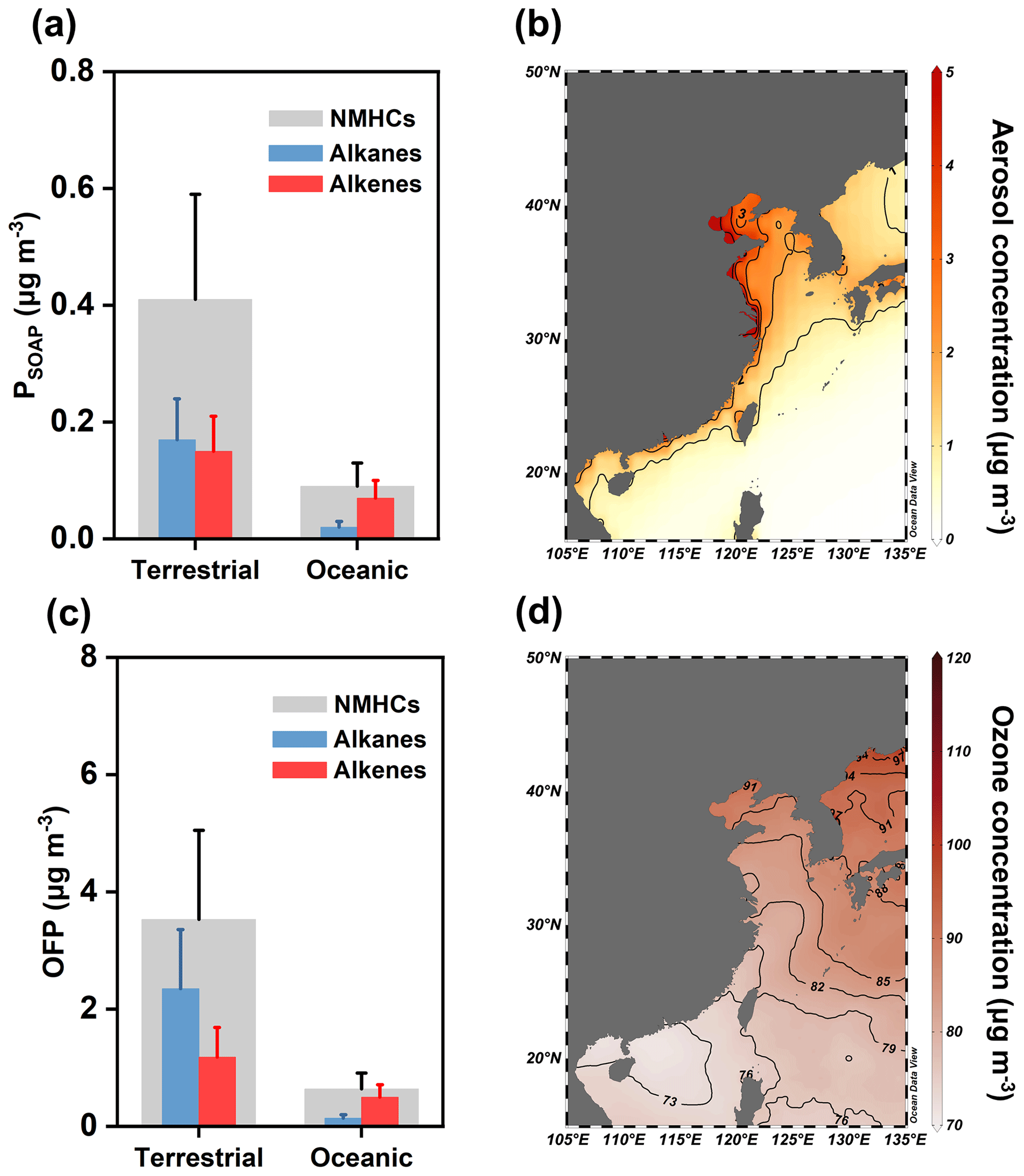
Figure 8 P_SOAP (a) and OFP (c) of NMHCs and averaged concentration of troposphere aerosol (b) and ozone (d) during the investigation period over the Chinese marginal seas. Data of aerosol (Global Modeling and Assimilation Office and Pawson, 2015) and ozone (Miyazaki, 2024) were downloaded from GES DISC (Schlitzer, 2023).

Similarly, the OFP of alkanes and alkenes from terrestrial sources was 2.35±1.01 and 1.18 ± 0.51 µg m⁻³, respectively, significantly higher than that from marine sources (0.14 ± 0.06 µg m⁻³ for alkanes and 0.50 ± 0.21 µg m⁻³ for alkenes) (Fig. 8c). However, the ozone distribution in the offshore atmosphere of China showed a decreasing trend from north to south (Fig. 8d). The marine atmosphere generally acts as a net ozone sink with ozone being primarily removed by photochemical degradation (Monks et al., 1998; Conley et al., 2011). The increasing solar radiation intensity from north to south enhances ozone degradation rates, likely dominating the ozone distribution in China's offshore atmosphere. Notably, satellite observations (GES DISC) during this investigation period indicated that the tropospheric ozone was approximately 82.6 ± 3.08 µg m⁻³ over the Chinese marginal seas. Among this, terrestrial C2–C5 NMHCs contributed around 4 % to total ozone concentration, suggesting a certain impact of terrestrial outflow on the tropospheric ozone in these regions.

4 Conclusions

Our study characterized the atmospheric NMHCs in both coastal cities and Chinese marginal seas and determined that both oceanic ventilation and terrestrial inputs play important roles in controlling the distribution and chemical composition of NMHCs in the coastal atmosphere of China.

Alkanes were the dominant NMHCs in both urban and nearshore atmospheres, and the atmospheric concentrations of alkanes were significantly higher in coastal cities compared to coastal seas, showing the potential of terrestrial alkanes as a source of alkanes in the marine atmosphere through transport. Generally, alkane concentrations tended to be higher in cases where the sampling sites were closer to land, there was a longer retention of air mass over land, and there was a shorter air mass transport time from land to the sampling site. However, these effects could not apply to alkenes due to their higher reactivities and the substantial sea-to-air fluxes. Additionally, the impact of oceanic emissions on NMHC composition was more pronounced in areas beyond 100 km from land compared to areas within 100 km because the terrestrial input gradually diminishes along the direction towards the open ocean.

Combining the outcomes of the PMF model and chemical profiles of diverse sources in the literature, we extracted four isolated sources of NMHCs in the nearshore atmosphere. Terrestrial sources (including industrial activities, vehicular exhaust, and vegetation emission) primarily constitute the NMHCs in the nearshore atmospheres, and they partially influence atmospheric SOA and ozone levels. This indicates the potential importance of terrestrial outflow in shaping the air quality and regulating climate dynamics in the marginal seas.