the Creative Commons Attribution 4.0 License.
the Creative Commons Attribution 4.0 License.
 | 01 Aug 2024
Environmental controls on isolated convection during the Amazonian wet season
Leandro Alex Moreira Viscardi
Giuseppe Torri
David K. Adams
Henrique de Melo Jorge Barbosa
The Amazon rainforest is a vital component of the global climate system, influencing the hydrological cycle and tropical circulation. However, understanding and modeling the evolution of convection in this region remain a scientific challenge. Here, we assess the environmental conditions associated with shallow, congestus, and isolated deep convection days during the wet season (December to April), employing measurements from the Green Ocean Amazon 2014–2015 (GoAmazon2014/5) experiment and large-scale wind fields from the constrained variational analysis. Composites of deep days show moister than average conditions below 3 km early in the morning. Analyzing the water budget at the surface through observations only, we estimated the water vapor convergence term as a residual of the water balance closure. Convergence remains nearly zero during the deep days until early afternoon (13:00 LST), when it becomes a dominant factor in the water budget. At 14:00 LST, the deep days experience a robust upward large-scale vertical velocity, especially above 4 km, which supports the shallow-to-deep convective transition occurring around 16:00–17:00 LST. In contrast, shallow and congestus days exhibit drier pre-convective conditions, along with diurnal water vapor divergence and large-scale subsidence that extend from the surface to the lower free troposphere. Moreover, afternoon precipitation exhibits the strongest linear correlation (0.6) with large-scale vertical velocity, nearly double the magnitude observed for other environmental factors, even moisture, at different levels and periods of the day. Precipitation also exhibits a moderate increase with low-level wind shear, while upper-level shear has a relatively minor negative impact on convection.
- Article
(6200 KB) - Full-text XML
- BibTeX
- EndNote


In the tropics, deep convection dominates the weather and climate. The formation of cumulus clouds and their evolution into cumulonimbus and often into mesoscale convective systems (MCSs) covers a wide range of spatial and temporal scales. Similarly, complex physical processes from cloud microphysics to gravity wave generation are intrinsically tied to deep convection (Mapes et al., 2006; Mapes and Neale, 2011; Jewtoukoff et al., 2013; Gupta et al., 2023). Representing these convective cloud processes in general circulation models (GCMs) is recognized as a source of bias and uncertainty (Sherwood et al., 2014; Stevens and Bony, 2013; Itterly et al., 2018; Maher et al., 2018; Freitas et al., 2020). In particular, the shallow-to-deep (STD) convective transition, whose physical mechanisms are still debated (Kuang and Bretherton, 2006; Khairoutdinov and Randall, 2006; Wu et al., 2009; Waite and Khouider, 2010; Schlemmer and Hohenegger, 2015; Morrison et al., 2022; Barber et al., 2022), has long been problematic for convective parameterizations (Betts, 2002; Betts and Jakob, 2002; Bechtold et al., 2004; Grabowski et al., 2006).
To evaluate model performance and to limit the uncertainty associated with the representation of deep convection that is either parameterized or resolved at the cloud scale, metrics derived from observations are required (Adams et al., 2013, 2017; Schiro et al., 2018; Barber et al., 2022). However, within the deep tropics, data are typically lacking at the resolution needed to evaluate parameterized convection in both GCMs and cloud-resolving models (CRMs), as well as to investigate the physical processes that drive mesoscale convective evolution. Intensive field campaigns such as the Green Ocean Amazon 2014–2015 (GoAmazon2014/5) experiment (Martin et al., 2016, 2017) have provided comprehensive measurements from the surface to the clouds, finally providing critical measurements of microphysical-scale to large-scale thermodynamic properties critical for studying convection (Giangrande et al., 2016, 2017, 2020; Barber et al., 2022).
Convective processes in the Amazon manifest themselves in two primary precipitation modes: isolated convection, which peaks in the late afternoon (around 16:00–17:00 LST), and organized convection associated with MCSs, which often peaks during the night into the early morning hours around 03:00–04:00 LST. This distinct cycle is pronounced in the southern (Tota et al., 2000; Machado, 2002; Silva Dias, 2002) and central (Greco et al., 1990; Adams et al., 2013; Ghate and Kollias, 2016; Giangrande et al., 2020) regions. In particular, isolated convection is tied to the diurnal cycle of thermodynamic and dynamical properties (Ghate and Kollias, 2016; Itterly et al., 2018; Zhuang et al., 2017; Tian et al., 2021). For example, using 3.5 years of water vapor fields from the Amazon Dense Global Navigation Satellite System (GNSS) Meteorological Network, Adams et al. (2013) observed a 4 h timescale of robust water vapor convergence associated with the STD transition regardless of convective strength, seasonal variations, or whether convection occurs during day or night. For the vertical moisture distribution, Ghate and Kollias (2016) noted that precipitating days in the dry season start the diurnal cycle by exhibiting a moister layer around 2–5 km. However, this contrasts with later studies, which observed that deep convection days are associated with a moister layer from the surface to the middle levels (∼ 5 km) (Zhuang et al., 2017; Tian et al., 2021).
Itterly et al. (2016) highlighted that convection in the Amazon region has a greater sensitivity to column water vapor, while convective available potential energy (CAPE) turns out to be an inadequate indicator of convection intensity. Further support for these findings comes from the work of Schiro et al. (2016, 2018), who demonstrated the necessity of incorporating deep-inflow mixing to accurately represent the entrainment of dry air in the parcel, which is essential for assessing the sensitivity of convection to instability. Itterly et al. (2018) reaffirmed the importance of the vertical distribution of humidity for the evolution of convection, but they showed that the relationship between convection and humidity is represented very differently in reanalysis data products. Previous studies have not provided conclusive evidence for the importance of vertical wind shear. For example, Zhuang et al. (2017) proposed that stronger lower- and upper-level bulk wind shear predominantly supports the STD transition but specifically during the dry season (June–September). In contrast, Chakraborty et al. (2018) proposed that increased low-level shear could hinder deep convection, particularly from August to November, especially if it leads to greater entrainment of dry air.
Although the above studies have used a combination of observational and reanalysis data to investigate different aspects of convection, they have not reached a consensus on which variables are most strongly associated with convective triggering or intensity in tropical regions. Here, we investigate the STD transition, employing data from the GoAmazon2014/5 rainy season observations. We analyze the diurnal cycle of days designated as shallow, congestus, and deep convection in terms of moisture, instability, and large-scale wind properties to assess the correlations of isolated convection in the Amazon with different environmental factors. In addition, we assess the correlation between conditionally averaged precipitation and these environmental factors to further determine their influence on convective intensity.
This paper is organized as follows: Sect. 2 presents an overview of the GoAmazon2014/5 data, followed by the derivation of the water budget and the procedures for convective regime classification. A comparison of cloud and precipitation properties among the shallow, congestus, and deep days is given in Sect. 3. Section 4 describes the diurnal cycle of the cloud regimes, while Sect. 5 presents the analysis of conditionally averaged precipitation based on different environmental controls. A discussion is provided in Sect. 6, and the conclusions are given in Sect. 7.
From January 2014 to December 2015, the GoAmazon2014/5 (Martin et al., 2016, 2017) experiment conducted the first long-term measurements of aerosols, clouds, and atmospheric thermodynamics in the central Amazon region. Nine ground sites and two aircraft were used to examine the environment in and around Manaus, a city that borders the Rio Negro and is surrounded by tropical rainforest. A detailed description of all sites can be found in Martin et al. (2016). This study focuses on the region around the most instrumented site, T3, located 70 km downwind of Manaus in Manacapuru (3.21° S, 60.60° W), where the ARM (Atmospheric Radiation Measurement) Mobile Aerosol Observing System (MAOS) and the ARM Mobile Facility 1 (AMF1) were deployed.
2.1 Experimental and large-scale data
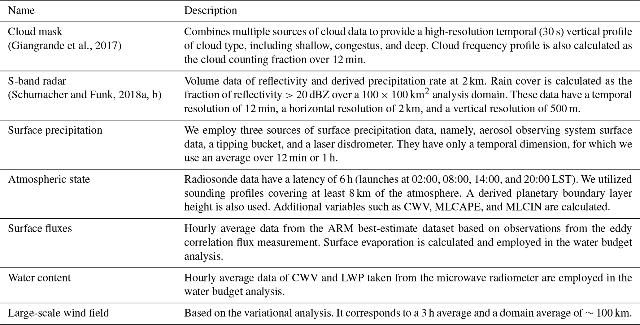
To begin our convective regime classification, described in the next section, we employed a cloud mask based on time–height profiles of the cloud location derived from the merged RWP-WACR-ARSCL cloud mask dataset, which combines the Radar Wind Profiler (RWP) data with the original W-band Cloud Radar (WACR) Active Remote Sensing of Cloud (ARSCL) value-added product (VAP), both located at T3 (Giangrande et al., 2017; Feng and Giangrande, 2018). This cloud mask identifies seven types of clouds, three of which correspond to convective clouds: shallow cumulus, with a base and cloud top below 3 km; congestus, with a base below 3 km and a top between 3–8 km; and deep convection, with a base below 3 km and a top > 8 km. From the cloud mask, available every 30 s, we also compute the cloud frequency profile in 12 min windows to match the S-band radar data described in the following.
The Amazon Protection System in Brazil (Sistema de Proteção da Amazônia, SIPAM) located at the T1 site (3.15° S, 59.99° W) operates an S-band (10 cm) Doppler single-polarization scanning radar south of downtown Manaus. We used the 12 min gridded reflectivity product with a horizontal resolution of 2 km and a vertical resolution of 500 m (Schumacher and Funk, 2018a). The S-band domain covers an area with a radius of 202 km. We use reflectivity profiles to assess rain coverage in our analysis domain, 100 × 100 km2 centered at the T3 site, calculated using a reflectivity threshold of 20 dBZ as in Zhuang et al. (2017). The surface precipitation rate is derived from the reflectivity of a constant altitude plan position indicator (CAPPI) at 2.5 km, calibrated with surface measurements from a Joss–Waldvogel disdrometer at the T3 site during the wet season of early 2014 (Schumacher and Funk, 2018b). In examining conditionally averaged precipitation (Sect. 5), the precipitation rate is averaged over the analysis domain along with an additional time average from 14:00 to 20:00 LST.
Figure 1 shows the map of S-band precipitation averaged over the wet season (December to April), 2014–2015. The precipitation statistics indicate that some radar beams are partially blocked. We used a threshold of 4 mm d−1 to roughly identify these problematic regions. Beam blockage affects only 7 out of 2601 pixels in our analysis domain, corresponding to only 0.3 %, with no relevant sensitivity to the chosen threshold. Although this contribution is negligible, we removed these blocked pixels from our analysis.
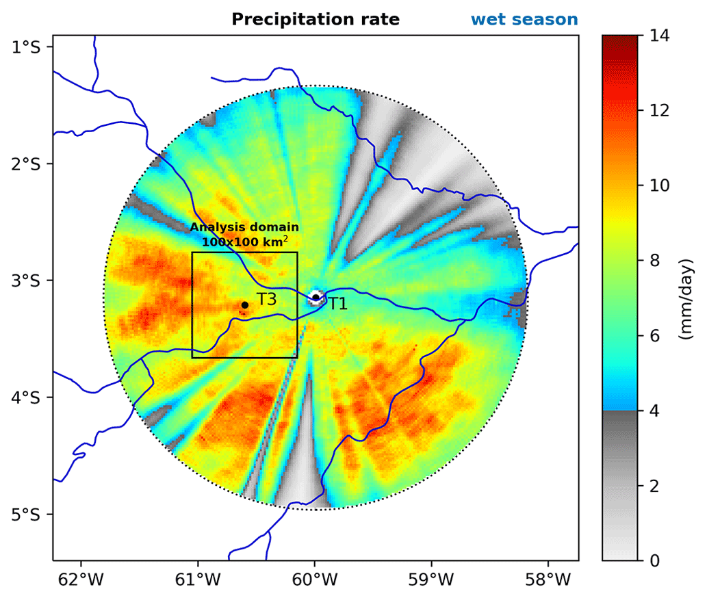
Figure 1Map of precipitation rate at 2.5 km in height averaged over the wet season (December to April), 2014–2015. The square box represents the analysis domain covering an area of 100 × 100 km2 centered at the T3 site. The dotted circle (radius of 202 km) centered over the T1 site indicates the domain covered by S-band radar measurements.
In addition to rain cover, the analysis of cloud and precipitation properties (Sect. 3) also uses the Aerosol Observing System Surface Meteorology (AOSMET) measured by the acoustic gauge of a Vaisala WXT520 station (ARM, 2013). A 12 min average is also applied to match the cloud frequency and S-band radar data.
The balloon-borne sounding system (SONDE) provides the vertical profiles of thermodynamic properties four times per day at 02:00, 08:00, 14:00, and 20:00 local standard time (LST; ARM, 2014f) during the wet season (December–April). For consistency, we analyze the atmospheric profile (potential temperature and humidity) only for soundings that extend from the surface to at least 8 km, and we linearly interpolate the profiles to a fixed 50 m vertical grid. The planetary boundary layer (PBL) height is derived from the profile of the bulk Richardson number using a critical threshold of 0.25 (ARM, 2014e). We also calculate additional variables from the thermodynamic profiles. The total column water vapor (CWV) is determined by integrating the water vapor mixing ratio from the surface to 350 hPa. For consistency, here we only analyze soundings that extend from the surface to at least 350 hPa (approximately 8.5 km). Similarly, the partially integrated CWV is calculated for the layers 1000–850 hPa (∼ 0–1.5 km; CWVlower), 850–700 hPa (∼ 1.5–3 km; CWVmid), and 700–350 hPa (∼ 3–8 km; CWVupper), which are representative of the convective boundary layer, lower free troposphere, and upper levels, respectively. Convective inhibition (CIN) and CAPE are also calculated. For these, a hypothetical air parcel is lifted dry adiabatically to the lifting condensation level (LCL) then pseudo-adiabatically from there. A mixed-layer parcel immediately above the surface, extending to a depth of 100 hPa, is used as the initial state for the parcel's ascent (Stull, 2017).
We used a combination of instruments to characterize the surface water budget. The latent heat flux is taken from the ARM best-estimate dataset (ARM, 2014a) based on observations from the Eddy Correlation Flux Measurement System (ECOR) (ARM, 2014b). Instead of using the S-band radar precipitation, the water balance analysis utilizes a combination of rain-gauge source measurements to provide a more robust estimation of the mean surface precipitation and its uncertainties. Specifically, we use the surface AOSMET precipitation (ARM, 2013), a tipping bucket (ARM, 2014g), and a laser disdrometer (ARM, 2014c). Here, CWV and liquid water path (LWP) are taken from the microwave radiometer (MWR; ARM, 2014d). Similarly to Schiro et al. (2016), we exclude data in cases where the brightness temperature surpasses 100 K and when water accumulates on the MWR lens surface during rainy periods. Hourly averages are applied for the data utilized in the water budget analysis, and the mathematical derivation is provided in the next section.
Large-scale wind properties and bulk vertical wind shear are analyzed by way of constrained variational analysis (VARANAL) data developed for the GoAmazon2014/5 experiment (Tang et al., 2016). This large-scale forcing dataset is derived from the European Centre for Medium-Range Weather Forecasts (ECMWF) analysis that is further constrained by S-band radar precipitation, surface fluxes, and Geostationary Operational Environmental Satellite (GOES-13) radiances. The VARANAL large-scale fields represent an average across an analysis domain centered at the S-band radar location, with a radius of 110 km.
Finally, a table summarizing the data is also provided in the Appendix (Table A1).
2.2 Derivation of the water budget
The integral form of the continuity equation for the total water rt can be written as
where p is pressure, g is gravity acceleration, V is the horizontal wind vector, and E and P correspond to the water mass fluxes associated with surface evaporation and precipitation. The total water rt is the sum of the three different phased-based mixing ratios, i.e., water vapor (rv), liquid (rl), and ice (ri). The second integral is the water mass flux divergence, which is mostly associated with the divergence of water vapor.
For the sake of this analysis, we neglect ice and express all terms in units of mm h−1. As we show later (Sect. 4.3), the results indicate a minor contribution of the liquid water term to the water budget, which supports ignoring the ice water term. Note that ice water paths are not necessarily smaller than the liquid water paths; however, they still encompass values of comparable orders of magnitude. Thus, the equation can be rewritten in a simplified form,
where EVAP corresponds to the evaporation rate, PREC corresponds to the precipitation rate, and CONV represents the water vapor convergence. Note that we intentionally rearranged the order of the equation to emphasize terms based on placing GoAmazon2014/5 observations on the left-hand side and placing the residuals, which can only be estimated, on the right-hand side. For this analysis, we consider only the hourly average of observed variables. Specifically, CWV and LWP are based on the MWR. ECOR latent heat flux data are utilized for estimating the evaporation term. Precipitation is obtained utilizing different sources, namely, aerosol observing system data, the tipping bucket, and the laser disdrometer (Sect. 2.1). We determine the mean of these sources and calculate the standard deviation from this sample mean. The water vapor convergence term is estimated using the mean composites for ∂tCWV (notation is used for convenience), ∂tLWP, EVAP, and PREC. The standard deviation of mean convergence is estimated from the standard deviation of the mean ∂tCWV, ∂tLWP, EVAP, and PREC, i.e., . Although this formula involves implicit assumptions, such as a lack of correlation among the variables in the square root, the uncertainty in the water budget is primarily attributed to ∂tCWV (see Fig. 9). Consequently, the uncertainty in the convergence term can also be roughly approximated by this term, with other terms contributing minimally.
Note that we only employed local surface measurements and applied hourly averages for the water budget datasets. Hence, the water balance is consistent over a temporal scale of an hour and a spatial scale on the order of meters. However, surface fluxes depend primarily on surface properties, which are approximately uniform around the experimental site, at least up to a distance of a few kilometers. Measurements of precipitation, CWV, and LWP are influenced by the cloud cover around the instrumentation location. Given that shallow-to-deep convection typically spans a spatial scale of approximately 1–10 km, our analysis is likely to generalize well across a spatiotemporal scale of 1 h and a few kilometers.
2.3 Convective regime classification
We define the wet season as the period from December to April, following previous studies in the central Amazon (Machado et al., 2004; Marengo et al., 2013). To contrast the different atmospheric conditions that lead to different convective regimes, we apply a classification criterion that identifies shallow, congestus, or deep days. Given our interest in convection that develops in response to the diurnal cycle, days with propagating mesoscale convective systems (MCSs) were excluded from our analysis. This regime classification follows the criteria proposed by Zhuang et al. (2017) and Tian et al. (2021). We first consider the diurnal period between 10:00–20:00 LST. Then, we define three categories of convective regimes: shallow cumulus, congestus, and deep, based on the maximum development of convective clouds during the diurnal cycle. The cloud mask from the RWP-WACR-ARSCL is used to identify cloud development throughout each day. In addition, we also employ rain coverage data from the S-band radar to estimate the vertical cloud development based on the echo cloud top. The rain coverage is calculated as the fraction of reflectivity pixels > 20 dBZ, regardless of whether the phase is ice or liquid (see Sect. 2.1). The echo top is defined as the highest level where rain coverage is greater than 2 %. The quantitative criteria are listed below.
- i.
Shallow convective days (ShCu). (1) The cloud mask does not show any congestus or deep clouds during the diurnal cycle (10:00–20:00 LST). (2) Rain cover above 3 km in altitude must be < 2 % in the analysis domain (100 × 100 km2, centered at T3).
- ii.
Congestus convective days (Cong). (1) The cloud mask indicates congestus clouds during the diurnal cycle, but none of them develop into deep clouds. (2) Rain cover above 8 km (between 3 to 8 km) in altitude must be < 2 % (> 2 %) in the analysis domain.
- iii.
Deep convective days (Deep). (1) The cloud mask indicates deep convection during the diurnal cycle. (2) Rain cover is above 8 km > 2 % in the analysis domain.
- iv.
Early-morning perturbation. For the 06:00–10:00 LST period, we require that no congestus or deep clouds be observed.
- v.
Local convection. No convective system with a contiguous area of precipitation > 10 000 km2 reaches the analysis domain between 06:00 and 20:00 LST.
Figures 2 and 3 illustrate the diurnal evolution of the occurrence of the different cloud types and rain coverage for the three regimes. The classification essentially depends on the cloud evolution during the diurnal cycle. The threshold of 2 % used to calculate rain cover is based on Zhuang et al. (2017), who manually tested several parameters. Their results indicated that shallow rain cover never exceeds 2 %, a criterion we adopted in our definition of minimum rain cover for identifying congestus or deep clouds. The exclusion of any relevant early-morning disturbance (06:00–10:00 LST) associated with important pre-convective activity guarantees that nighttime MCSs do not cause significant preconditioning.
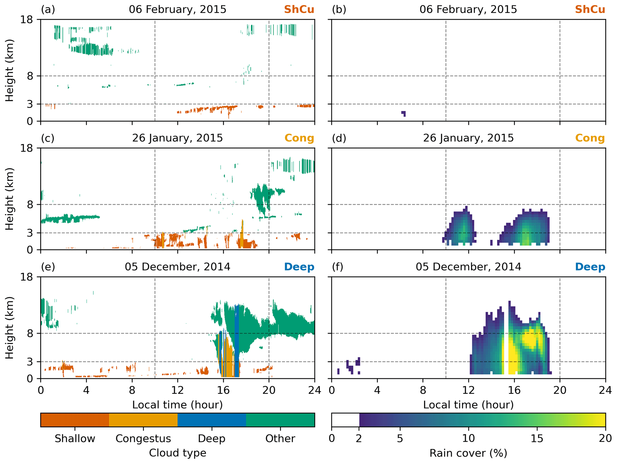
Figure 2Cloud mask (a, c, e) and rain coverage (b, d, f) for examples of days classified as shallow (ShCu; a–b), congestus (Cong; c–d), and deep (Deep; e–f).
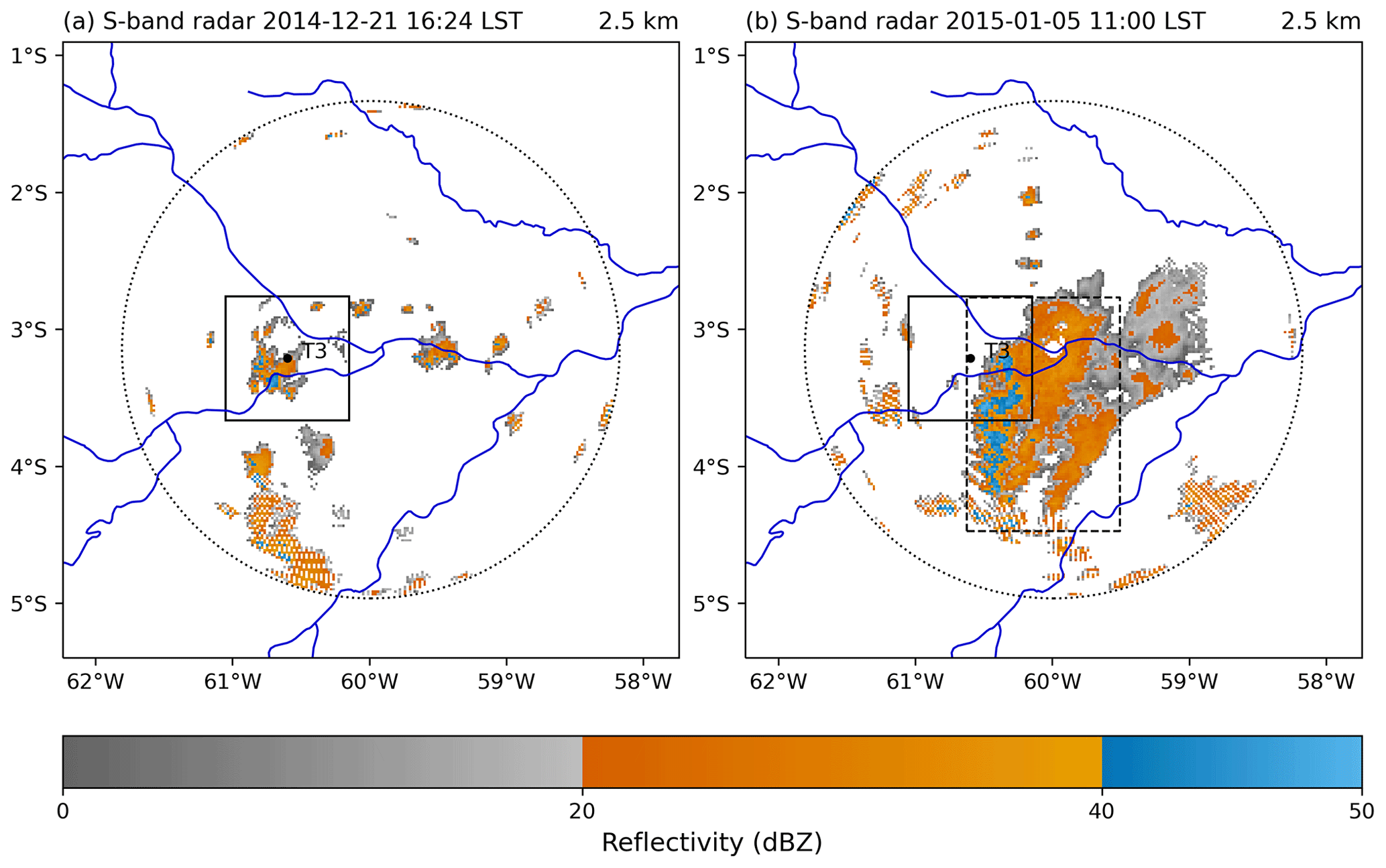
Figure 3Convective systems. (a) Scattered local system. (b) Non-local propagating system. The dashed black box illustrates the region with a contiguous area of precipitation (> 20 dBZ) not fulfilling the local convection requirement.
The number of days categorized according to the above criteria for the wet season (blue) and dry season (red) is shown in Fig. 4. Deep convection appears to be the dominant category in both seasons, although the propagating-convection category occurs more frequently during the wet season. Specifically, we identified 16 d for the ShCu regime, 27 d for the Cong regime, 60 d for the Deep regime, and 111 d for non-local (organized) deep convection. Given our focus on the local shallow-to-deep transition mechanism during the wet season, the results presented in the next section refer only to those 103 d.
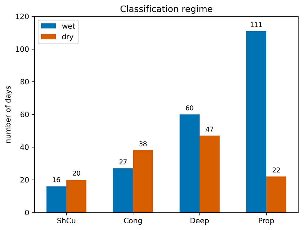
Figure 4Number of days classified in each convective regime during the wet (December–April) and the dry (June–August) seasons from 2014 to 2015. Propagating (prop) days refer to non-local deep convection, with the early-morning perturbation condition being ignored.
The composite diurnal cycles of the vertical cloud frequency profiles, local surface precipitation rate, and rain coverage for the different convective regimes are shown in Fig. 5. For all convective regimes, daytime convection is usually preceded by some nighttime cloud cover at all levels.
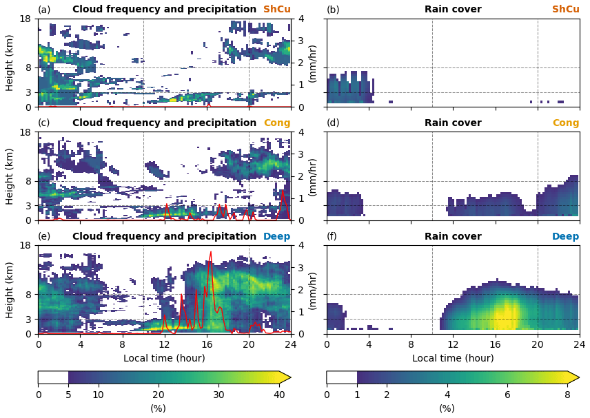
Figure 5(a, c, e) Cloud frequency (cloud counting fraction in %, color map) as a function of height calculated over a 12 min window based on the cloud mask and surface precipitation rate (mm h−1, red line) measured locally by the aerosol observing system at the T3 site. (b, d, f) Rain cover (%) over the analysis domain (100 × 100 km2, centered at T3) based on the S-band radar. The mean composites distinguish days classified as shallow (a–b; N=16), congestus (c–d; N=27), and deep (e–f; N=60) during the wet season.
The ShCu regime has a more scattered cloud frequency during the daytime. Low-level clouds dominate the diurnal cycle, with a peak reaching 54 % at 1.43 km around 13:00 LST. After 17:00 LST, cirrus clouds also contribute to the cloud frequency composite, likely transported from afar. The local surface precipitation rate remains below 0.13 mm h−1 throughout the diurnal cycle, while the rain cover has only a minor contribution of approximately 1 % at the end of the day.
The Cong regime also shows a higher cloud frequency below 3 km during the diurnal cycle. The maximum cloud cover is 50 % at 1.04 km around 12:00 LST, earlier and lower than that observed for the ShCu regime. Between 3 and 8 km, the cloud frequency composite has values below 5 %. Surface precipitation occurs around 12:00 LST, corresponding temporally to the period of maximum cloud cover. Nonetheless, the magnitude remains modest, with precipitation values at less than 0.75 mm h−1 throughout the diurnal cycle. Contrary to the local cloud frequency assessed at the T3 site, the domain rain coverage exhibits a distinct pattern at the middle levels, indicating values of 1 %–2 %. After the diurnal cycle, the rain coverage composite indicates that congestus clouds may evolve into a deeper phase. We identified seven cases (26 %) in which congestus days fulfilled the Deep criteria (echo top above 8 km) after the diurnal cycle.
The Deep regime reveals a more coherent cloud frequency profile associated with more extensive and longer-lived convective clouds during daylight hours. The maximum Deep cloud frequency is also associated with shallow clouds: 49 % at 0.92 km around 11:30 LST. As we discuss next, this is associated with the boundary layer height and the lifting condensation level both being lower in the Deep regime. As the day progresses, the Deep cloud frequency also increases throughout the troposphere, with the cloud top reaching up to 16 km. After cumulonimbus dissipation (around 18:00 LST), its anvil structure remains and may become a cirrus cloud that may contribute to the cloud cover of the next day. Surface precipitation typically occurs around noon and in the afternoon as clouds develop. Notably, substantial rain coverage emerges between 16:00 and 17:00 LST, with a maximum surface precipitation of 3.72 mm h−1 peaking at 16:24 LST. This occurrence is consistent with the late afternoon STD transition in the Amazonian wet season.
In this section, we specifically evaluate the environmental conditions associated with the STD convective transition. We analyze the local atmospheric conditions, convective properties, surface water balance, and large-scale wind properties associated with shallow, congestus, and deep convective days. To account for the small sample size associated with the classification of the convective regime (Fig. 4), we employed the bootstrap method, utilizing 50 000 samples to estimate the mean and standard deviation for each composite. These are represented by the line and error bars in each figure in this section.
4.1 Atmospheric conditions
Figure 6 shows the average vertical profiles of potential temperature (Fig. 6a), θ, and water vapor mixing ratio (Fig. 6b), rv, for each convective regime at 08:00 LST. The differences between the Deep and the other convective regimes, Δθ and Δrv, are shown in panels (c)–(d).
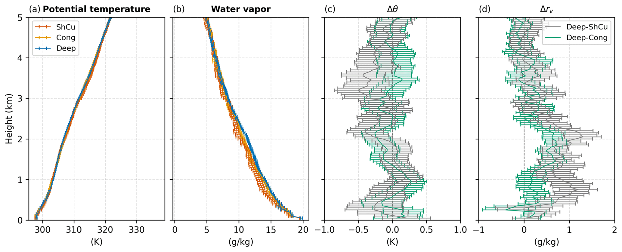
Figure 6Atmospheric conditions. (a) Potential temperature (K) and (b) water vapor mixing ratio (g kg−1) from 08:00 LST radiosonde observations. The corresponding convective regime differences (Deep − ShCu and Deep − Cong) for potential temperature (Δθ; c) and mixing ratio (Δrv; d) are also included. The error bars in (c) and (d) are obtained from the bootstrap standard error in the convective regimes, i.e., .
The potential temperature differences between the convective regimes are frequently less than 0.5 K below the 8 km level, suggesting that there is no relevant relationship between daytime cloud development and the morning temperature profile. The Deep regime experiences higher moisture content, especially below 3 km. The most remarkable difference occurs around the 2 km level, with Δrv reaching 1.30 and 0.74 g kg−1 for Deep − ShCu and Deep − Cong, respectively. Above 3 km, the differences in moisture profile for all regimes are minimal.
These results suggest that the importance of early morning excess humidity to the STD transition in the Amazon is primarily limited to the lower levels, a finding supported by Zhuang et al. (2017) and Tian et al. (2021). However, it differs from Ghate and Kollias (2016), who noted an excess of humidity solely above 2 km during precipitating days in the dry season. Moreover, these results contrast with studies over tropical oceans, where free-tropospheric humidity has been shown to play a more significant role in convective activity, while boundary layer humidity demonstrates minor variability (Bretherton et al., 2004; Holloway and Neelin, 2009).
The column water vapor (CWV) for each radiosonde time is presented in Fig. 7a, while panels (b)–(d) show the partial contribution from lower, middle, and upper levels (see Sect. 2.1). The ShCu regime shows smaller CWV throughout the day. The difference between Deep and ShCu ranges from 2.3 mm at night to 5.1 mm at 14:00 LST. The differences in CWV between the Cong and Deep regimes are minimal from nighttime to early morning, while their difference is at a maximum at 14:00 LST, when it reaches 2.1 mm.
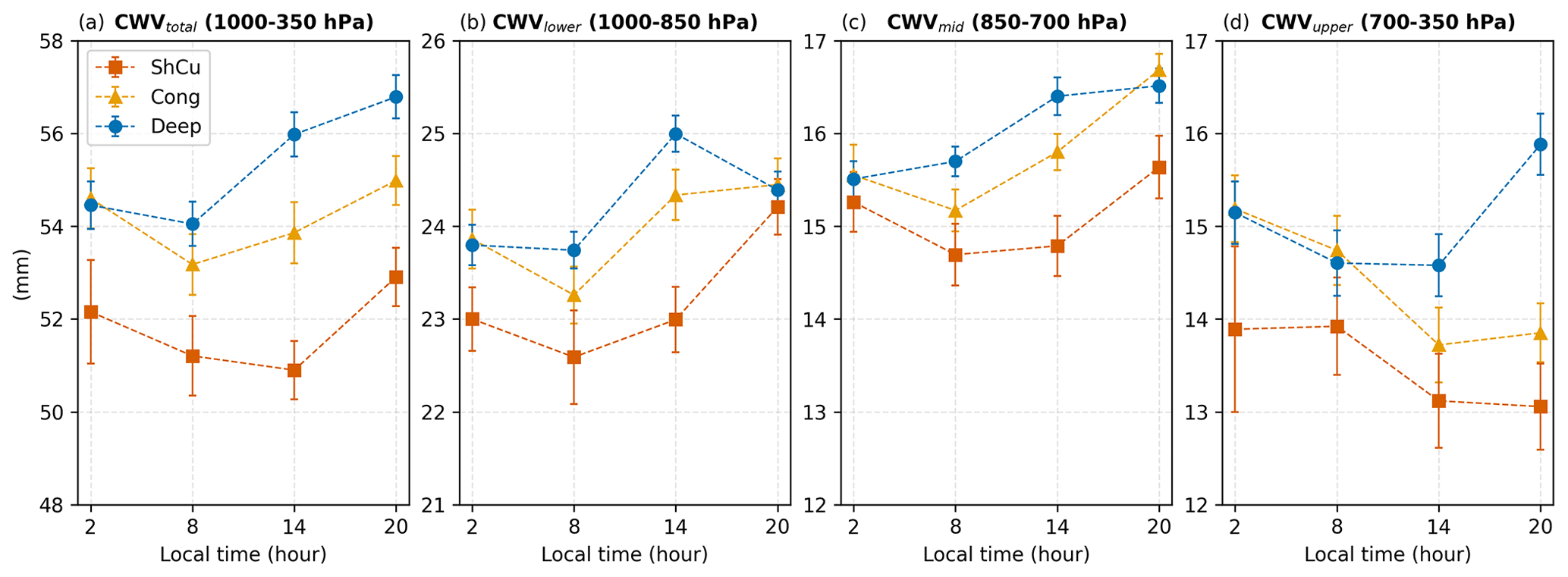
Figure 7Column water vapor (CWV; mm) at the radiosonde launch times (02:00, 08:00, 14:00, and 20:00 LST). (a) Total CWV and its partial contribution to the (b) 1000–850 hPa, (c) 850–700 hPa, and (d) 700–350 hPa layers.
CWVlower increases from 08:00 to 14:00 LST for all convective regimes. This increase is possibly due to evapotranspiration, which appears to be the dominant moisture factor during this period (water budget analysis, Sect. 4.3). A similar, albeit less pronounced, diurnal moistening is also observed in CWVmid for all regimes. However, the upper-level CWV is essentially constant for the Deep regime in the 08:00–14:00 LST period, while the ShCu and Cong regimes show a decrease of 0.80 and 1.02 mm, respectively. This indicates that the ShCu and Cong regimes might be associated with large-scale subsidence (see Sect. 4.4), which would explain the drying of the middle levels. Moreover, we note that Deep days show a significant increase in CWVupper from 14:00 to 20:00 LST, with a simultaneous decrease in CWVlower. This is likely due to a combination of water vapor convergence (Sect. 4.3) preceding the late afternoon STD transition and the vertical transport of moisture by deep clouds.
4.2 Convective properties
Figure 8 shows the PBL height, the mixed-layer convective inhibition (MLCIN), and mixed-layer convective available potential energy (MLCAPE). The PBL height among the convective regimes differs the most at 14:00 LST, when the convective boundary layer roughly coincides with the LCL or cloud base height (not shown), being about 500 m lower for the Deep (1535 m) than for the ShCu (1998 m) regime. The most developed convective regimes show a combination of higher MLCAPE and lower MLCIN in the early morning, providing more buoyancy and a lower barrier for convection to develop. At 14:00 LST, MLCAPE for the Deep regime (1074 J kg−1) and Cong regime (986 J kg−1) significantly exceeds the value for the ShCu regime (558 J kg−1). The change in MLCAPE from afternoon to early evening (MLCAPE(20:00 LST) − MLCAPE(14:00 LST)) is negative for the Deep regime (−138 J kg−1) and positive for the Cong (139 J kg−1) and ShCu (644 J kg−1) regimes. As expected, convection in more advanced stages consumes MLCAPE more effectively, reducing atmospheric instability.
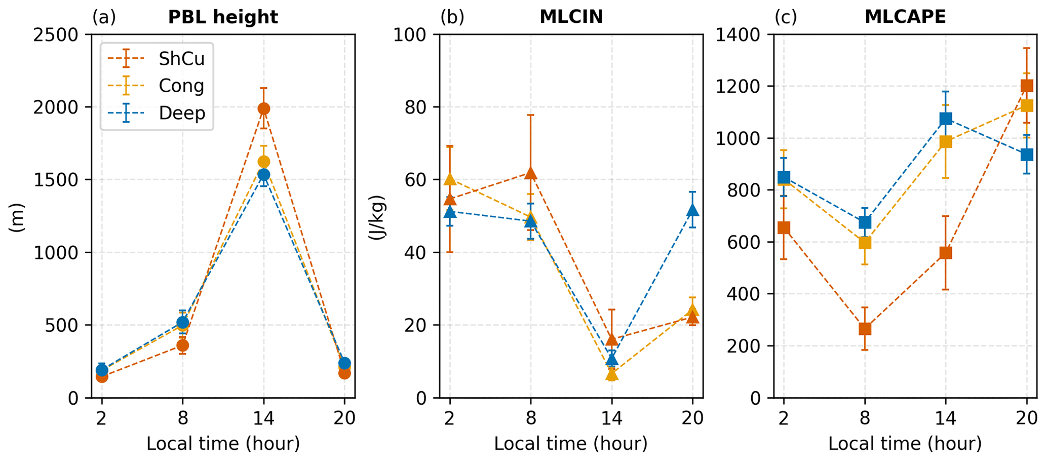
Figure 8(a) Planetary boundary layer (PBL) height (m), (b) 100 hPa mixed-layer convective inhibition (MLCIN; in J kg−1), and (c) 100 hPa mixed-layer convective available potential energy (MLCAPE; in J kg−1) at the radiosonde launch times (02:00, 08:00, 14:00, and 20:00 LST).
4.3 Surface water balance
To understand how the differences in the surface fluxes change CWV, affecting the STD transition and the accumulated surface precipitation, we analyzed the surface water balance (see Sect. 2.2).
The water balance results are shown in Fig. 9, with panels (a)–(c) showing the hourly average rate values (mm d−1) and panels (d)–(f) showing the corresponding accumulated values (mm). The separate precipitation and convergence associated with each rain gauge used to estimate the mean surface precipitation and the uncertainty in the water budget results are provided in Fig. A1 in the Appendix. First, we notice that the ∂tLWP appears negligible, and it does not contribute significantly to the water budget. The daytime of ShCu and Cong days shows mostly water vapor divergence. This is primarily due to more significant negative changes in ∂tCWV and low precipitation rates, as evaporation shows smaller differences among the convective regimes, and changes in ∂tLWP exert a minor influence on the water budget. On the other hand, the Deep regime exhibits relatively neutral conditions from night to early afternoon. However, the water budget closure requires convergence in the period from 14:00 to 18:00 LST. This coincides with the STD transition and is thus primarily attributed to strong water vapor convergence preceding the late afternoon STD transition (Adams et al., 2013, 2017). At the end of the day, the ShCu regime is estimated to lose 3.4 mm of water vapor due to divergence, while the Cong regime loses 0.9 mm. In contrast, the Deep regime gains 5.2 mm of water vapor due to convergence.
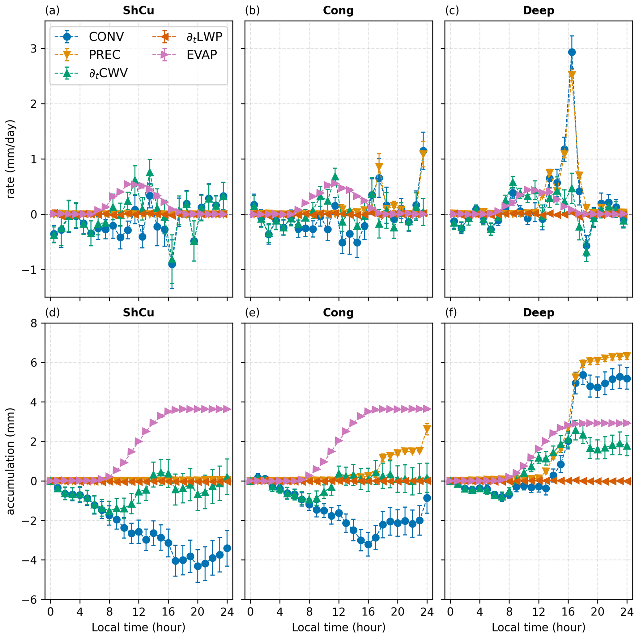
Figure 9Surface water balance for the (a, d) ShCu regime, (b, e) Cong regime, and (c, f) Deep regime. Panels (a–c) represent the rates of change (mm d−1) for water vapor convergence (CONV), evaporation (EVAP), precipitation (PREC), and the time derivatives of column water vapor (∂tCWV, where ) and the liquid water path (∂tLWP). Panels (d–f) display the accumulated water amount for each term in the water budget during the day (mm). Note that CWV and LWP changes rely on microwave radiometer observations, evaporation on eddy correlation flux measurements, and precipitation on estimations utilizing different sources, namely the aerosol observing system surface data, a tipping bucket, and a laser disdrometer. The water vapor convergence term is estimated as a residual in the water budget equation (Eq. 2).
For ShCu days, relatively high surface evaporation and the absence of precipitation require a strong divergence for water balance closure. The Cong regime shows a significant divergence but is relatively weaker compared to the ShCu regime, as their surface evaporation fluxes are relatively similar, and congestus precipitation exhibits modest values. For ShCu days, the ∂tCWV tends to be small and negative from nighttime to early morning. Then, it increases and balances around noon. By the end of the day, the accumulation of water vapor (Fig. 9d) in the column is negligible. This term is also nearly zero during Cong days. Conversely, the convergence of vapor and evaporation exceeds the precipitation term on Deep days, resulting in a net accumulation of 1.8 mm of column water vapor, which might act as positive feedback for the continuation of nocturnal deep convection into the following day after Deep regime conditions. This particular finding had not been previously addressed in studies utilizing the GoAmazon2014/5 observations.
4.4 Large-scale wind properties
Figure 10 displays the wind speed at 08:00, 11:00, and 14:00 LST for all convective regimes. The wind profiles for all regimes peak between the 900 and 800 hPa layer, characteristic of the low-level jet also reported by Anselmo et al. (2020), which they observed 10 %–40 % of the time during GoAmazon2014/5 between March and May 2014–2015. During the morning, the ShCu regime reveals a lower and slightly stronger jet. However, the PBL grows during the day to a height of 1–2 km (see Fig. 8), reaching higher altitudes for ShCu days, and the mixing of free-tropospheric and PBL momentum potentially reduces the wind speed. As a result, the lower jet in the ShCu regime is likely influenced more by the PBL growth compared to other regimes. Thus, at 14:00 LST, the ShCu regime reveals a less prominent low-level wind peak but at a slightly higher altitude compared to Deep days. For the middle and upper levels between the 600 and 350 hPa layers, the ShCu regime shows an additional upper-level maxima, while the Cong and Deep regimes exhibit weaker and comparable wind speeds, respectively.
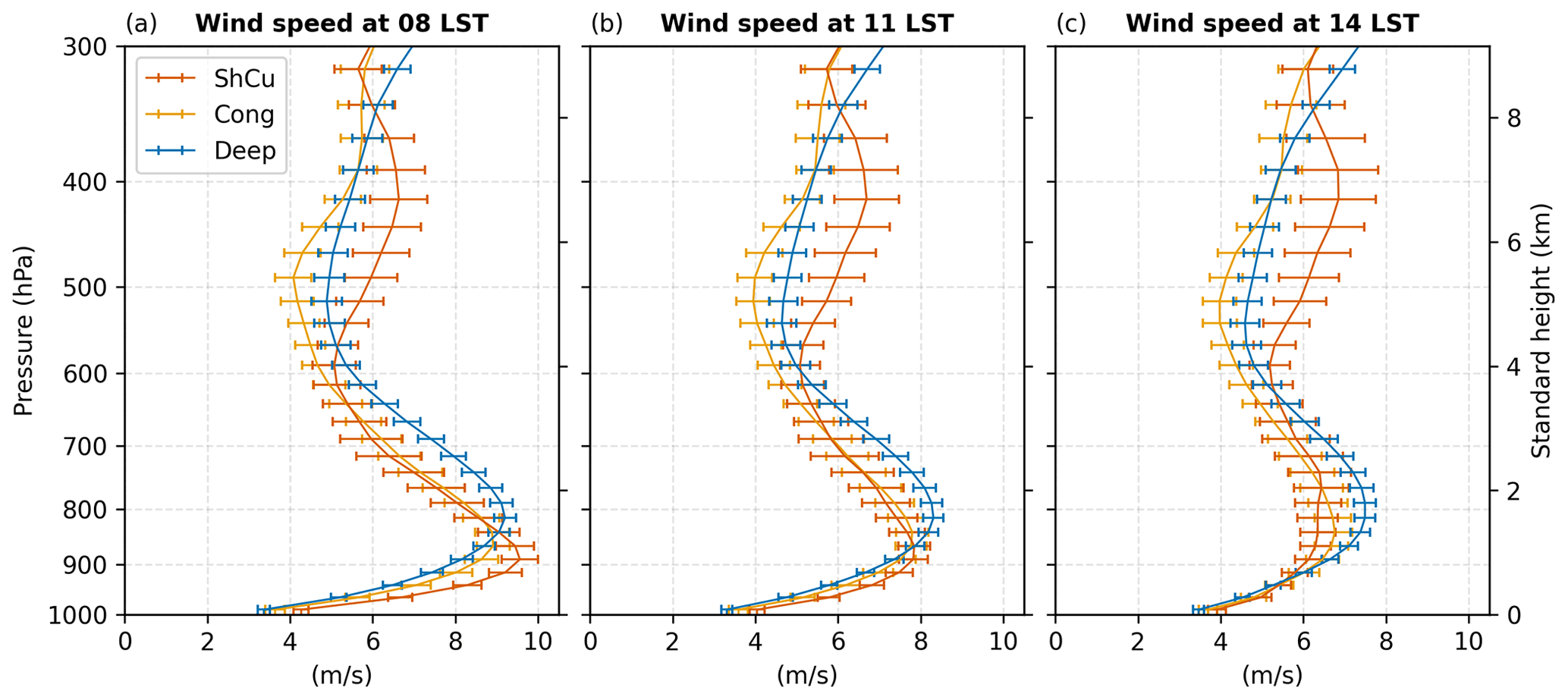
Figure 10Large-scale horizontal wind speed (m s−1) at (a) 08:00 local standard time (LST), (b) 11:00 LST, and (c) 14:00 LST for the ShCu, Cong, and Deep regimes.
A hodograph at 14:00 LST is displayed in Fig. 11. The wind turns clockwise with increasing height: northeasterly winds dominate in the boundary layer, approximately below 800 hPa, while easterly winds dominate in the ∼ 700–500 hPa layer. The most notable difference in wind direction occurs in the upper troposphere above 400 hPa. On the Deep days in particular, the wind stops veering, demonstrating a consistent southeasterly direction. Since the wind profiles at lower and middle levels are comparable among the convective regimes, the veering of the wind alone only hints at a possible control mechanism for the development from the congestus to the deep phase.
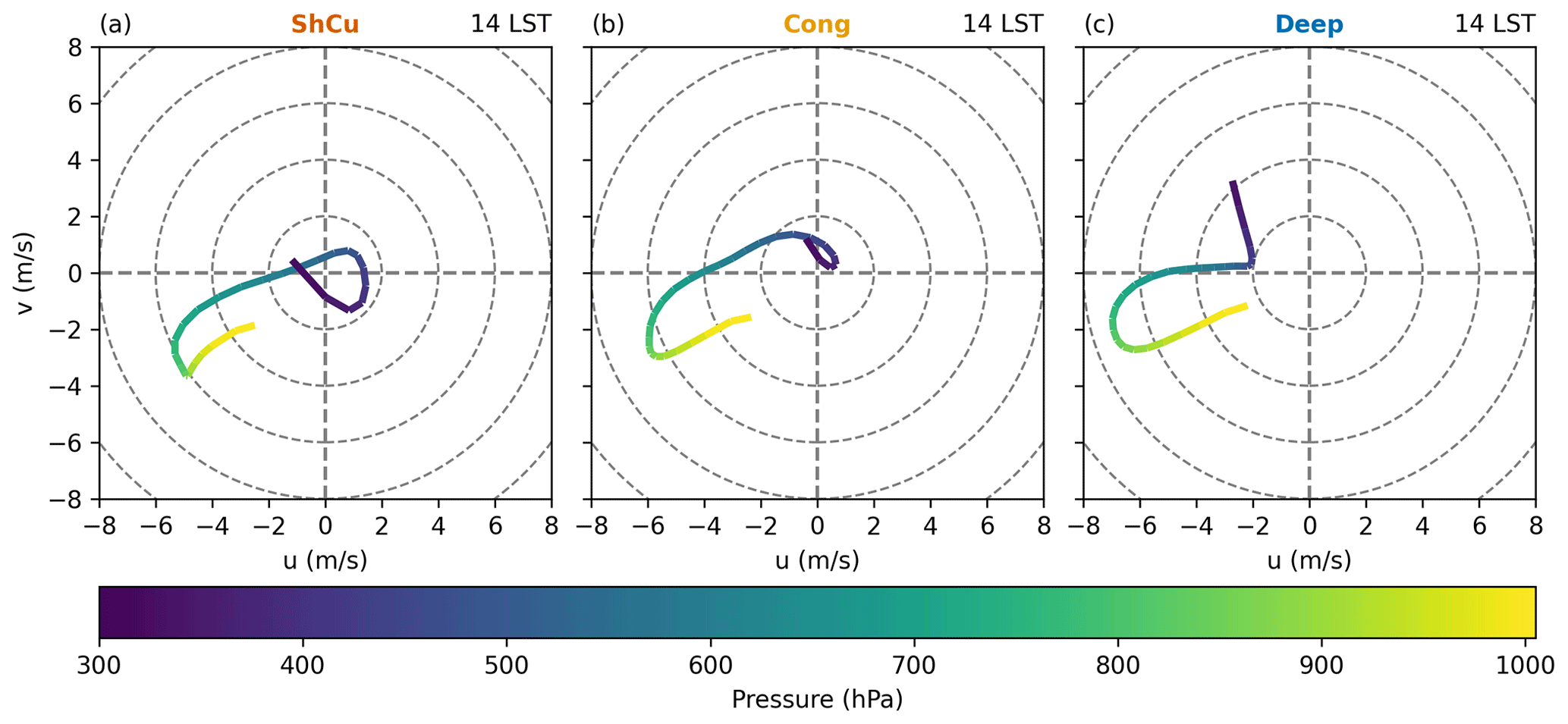
Figure 11Hodograph representing the u (m s−1) and v (m s−1) large-scale wind components as a function of pressure at 14:00 LST for the (a) ShCu regime, (b) Cong regime, and (c) Deep regime.
Figure 12 contains the large-scale vertical velocity (ω in hPa h−1) from the variational analysis at 08:00, 11:00, and 14:00 LST. In the early morning, the Deep regime shows moderate upward large-scale vertical velocity below 700 hPa, relatively greater than the velocities associated with the ShCu and Cong regimes. Above 700 hPa, ω becomes positive (subsidence) and exhibits comparable values among the convective regimes. Around noon (11:00 LST), the Deep regime is dominated by upward large-scale vertical velocity below 600 hPa, while the ShCu and Cong regimes exhibit similar ω profiles, with subsidence dominating above the surface. In the afternoon, significant differences are observed between the convective regimes. The Deep regime is dominated by upward large-scale vertical velocity, especially above the 800 hPa level. The ShCu and Cong regimes exhibit important subsidence in the lower levels, particularly below 700 hPa, with ShCu subsidence assuming higher magnitudes. Tian et al. (2021) also reported a significant disparity in the large-scale vertical velocity between Deep and ShCu days, especially in the afternoon and early evening.
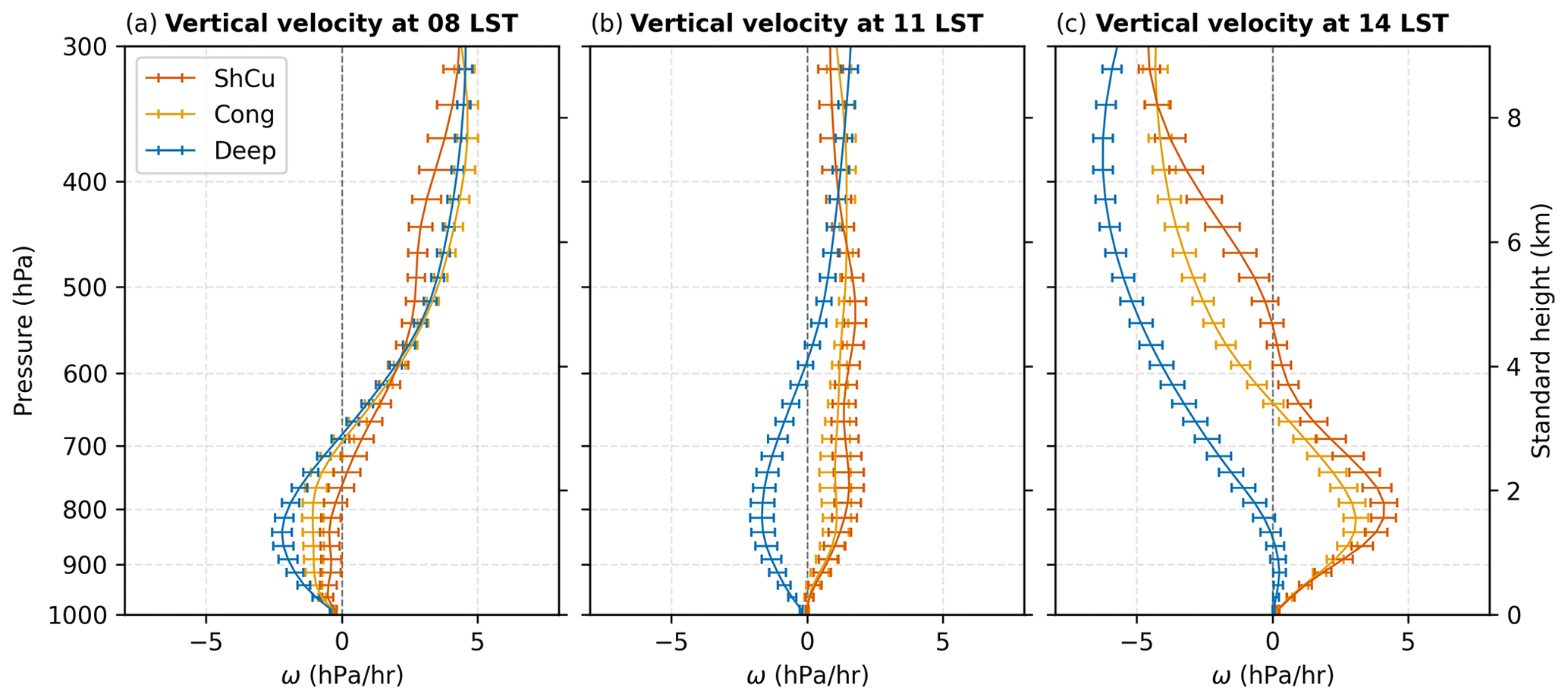
Figure 12Large-scale vertical velocity (ω in hPa h−1) at (a) 08:00 LST, (b) 11:00 LST, and (c) 14:00 LST for the ShCu, Cong, and Deep regimes.
To evaluate the vertical wind shear, we used the bulk wind shear, which is defined as the magnitude of the vector difference in the wind at two levels. Figure 13 shows the vertical bulk wind shear for the layers 0–2, 0–4, and 0–6 km. Additionally, the bulk shear from the level of maximum wind speed below 4 km and the associated pressure level are provided in Fig. A2. The 0–2 km layer exhibits a greater dependence on the diurnal cycle, with the Deep days (followed by Cong days) showing the most substantial wind shear at any time. Moreover, the Deep regime shows the largest difference between the maximum wind speed below 4 km and the surface wind. These results suggest that low-level vertical wind shear is related to convection development. For the 0–4 km layer, the wind shear is more similar between the convective regimes. For the 0–6 km layer, the Cong and Deep regimes exhibit similar patterns, while ShCu days are characterized by larger wind shear values and greater variability.
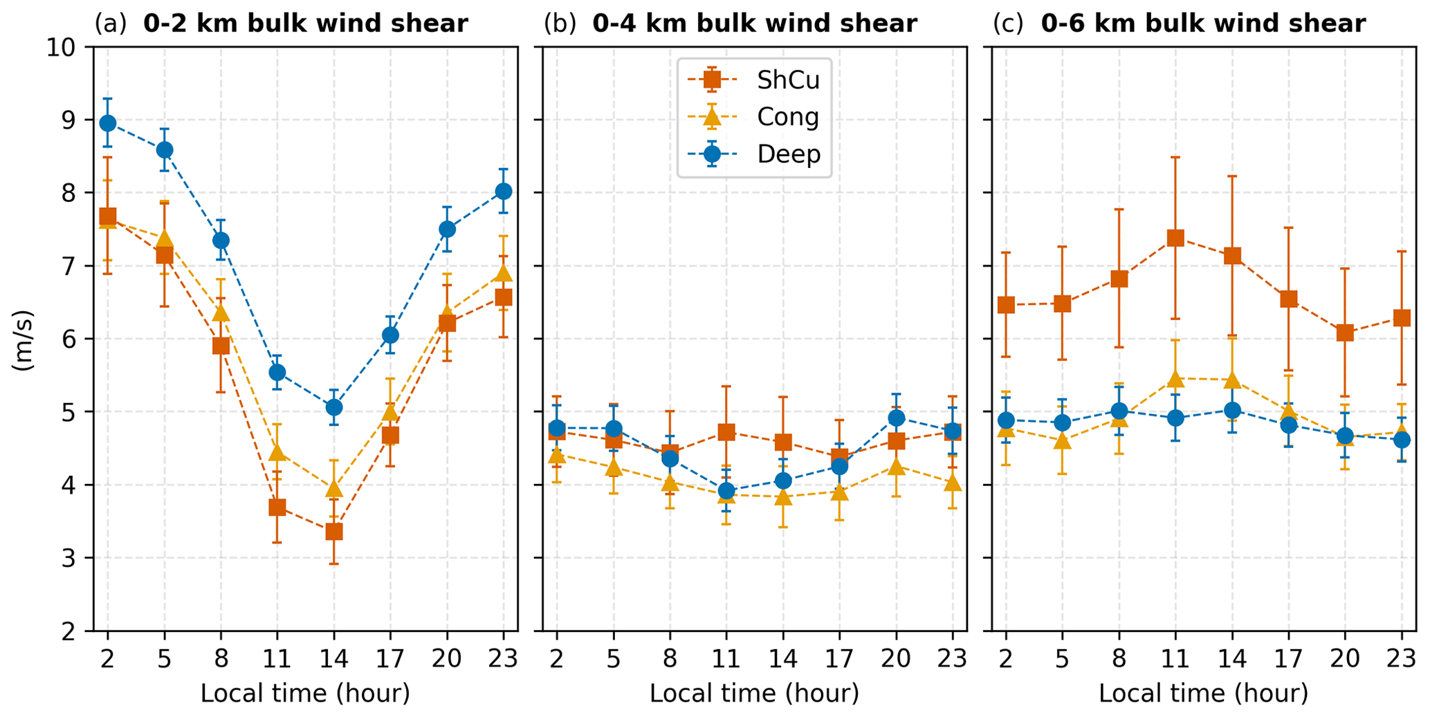
Figure 13Vertical bulk wind shear (m s−1) for the layers (a) 0–2 km (surface–790 hPa), (b) 0–4 km (surface–615 hPa), and (c) 0–6 km (surface–465 hPa).
In this section, the conditionally averaged precipitation is evaluated as a function of the main variables presumed to control the STD transition. From the previous section, we observed that convective development is primarily associated with humidity at lower levels in the early morning, while in the afternoon, it is more strongly related to upper-level moisture, instability, large-scale vertical velocity, and vertical wind shear.
Here, we explore the precipitation response to moisture using low-level and lower-free-troposphere CWV at 08:00 LST, upper-level CWV at 14:00 LST, MLCAPE at 14:00 LST, mean vertical velocity in the 1000–700 and 700–300 hPa layers at 14:00 LST, and bulk shear magnitude for the 0–2 and 0–6 km layers at 14:00 LST as surrogates for vertical wind shear. Precipitation from S-band radar is averaged over the analysis domain (100 × 100 km2 centered at T3) and from 14:00 to 20:00 LST. The conditionally averaged precipitation corresponds to the average precipitation observed within distinct bins for each variable, which were defined as 1 mm for CWV, 2.5 J g−1 (2500 J kg−1) for MLCAPE, 1 hPa h−1 for vertical velocity, and 2 m s−1 for bulk shear magnitude. In this analysis, it is important to highlight that we group the ShCu, Cong, and Deep regimes together and consider them collectively as local convective days.
Figure 14 consists of the conditionally averaged precipitation analysis. Large-scale afternoon vertical velocity exhibits the strongest correlation with precipitation: −0.596 in the 700–300 hPa layer and −0.570 in the 1000–700 hPa layer. Above 3 km (700–300 hPa), precipitation increases significantly, from nearly zero to approximately 0.8 mm h−1 as vertical motion rises from nearly zero to about −9 hPa h−1. These correspond to the heaviest conditionally averaged precipitation rates. Interestingly, vertical wind shear, especially the low-level (0–2 km) bulk shear magnitude, exhibits the second-strongest correlation with precipitation, although it has a modest value (0.348).
The lower-free-troposphere CWV at 08:00 LST demonstrates a similar correlation (0.311) with precipitation. The correlations for low-level CWV at 08:00 LST (0.274) and upper-level CWV at 14:00 LST (0.254) are also comparable. Vertical wind shear at higher levels (0–6 km layer) exhibits a weak negative correlation (−0.099) with precipitation. On the other hand, bulk shear in the 0–4 km layer (0.016) and MLCAPE (0.055) exhibit the smallest correlation values, which increase only weakly with precipitation. These results suggest that CAPE is not a good indicator of precipitation in the Amazon, which is consistent with the findings of Itterly et al. (2016) and Schiro et al. (2018). Thus, days starting with excess water vapor in the lowest 3 km of the troposphere and exhibiting relatively stronger large-scale vertical velocity and low-level wind shear in the afternoon have the highest probability of developing deep afternoon convection accompanied by heavy precipitation.
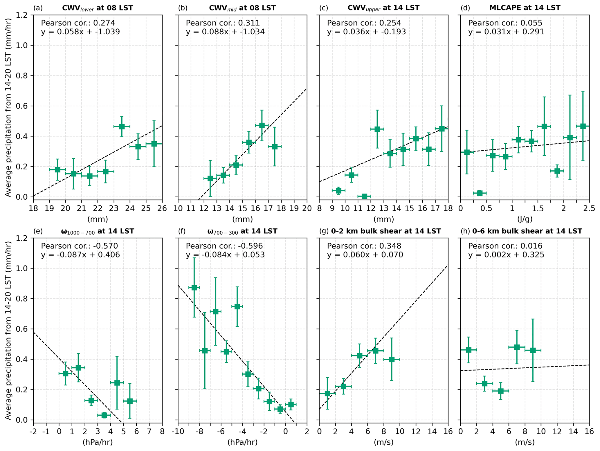
Figure 14Conditionally averaged precipitation (mm h−1) to (a) low-level column water vapor (CWV; in mm) at 08:00 LST, (b) lower-free-troposphere CWV at 08:00 LST, and (c) upper-level CWV at 14:00 LST. The (d) 100 hPa mixed-layer convective available potential energy (MLCAPE; in J g−1) at 14:00 LST. Mean large-scale vertical velocity (ω; in hPa h−1) in the (e) 1000–700 hPa and (f) 700–300 hPa layers at 14:00 LST and bulk wind shear magnitude (m s−1) in the (g) 0–2 km layer and (h) 0–6 km layer at 14:00 LST. Precipitation corresponds to the mean S-band radar precipitation from 14:00 to 20:00 LST. The bins for averaging each variable are indicated by horizontal bars, which represent 1 mm for CWV, 2.5 J g−1 (2500 J kg−1) for MLCAPE, 1 hPa h−1 for vertical velocity, and 2 m s−1 for wind shear. The conditional averaging analysis is conducted for local convective days (ShCu, Cong, and Deep regimes) indicated by green square markers. Additionally, linear least-squares regressions and Pearson correlations are included for each analysis.
The previous section presented the wet-season composites of ShCu, Cong, and local Deep convection days for both environmental and cloud properties measured during the GoAmazon2014/5 campaign. Cumulonimbus clouds can extend up to 16 km in altitude, and precipitation peaks around 16:00–17:00 LST, associated with the STD transition. This is consistent with previous studies in the southern Amazon. For example, Tota et al. (2000) and Machado (2002) analyzed data from the Wet Season Atmospheric Mesoscale Campaign (WETAMC) from January to February 1999 and reported two main precipitation modes: isolated convection, which peaks in the afternoon around 16:00 LST, and organized convection associated with mesoscale convective systems, with a maximum during the night around 04:00 LST. The diurnal peak associated with deep convection has also been documented more recently in Ghate and Kollias (2016) and Tian et al. (2021), who also used the GoAmazon2014/5 observations but did not focus on the wet season as in our study.
Our results show that deep days are associated with moister conditions in the early morning but only in the lower troposphere, particularly below 3 km. This contrasts with the results from Itterly et al. (2016). They also noted significant differences between morning atmospheric conditions and convective intensity but indicated that humidity in the upper troposphere also exhibits a strong relationship to convective intensity. The work by Ghate and Kollias (2016) focused on GoAmazon2014/5 observations during the dry season and observed the presence of an early morning moist layer (but elevated) between 2 and 5 km. In contrast, Zhuang et al. (2017) and Tian et al. (2021) found that days with deep convection exhibited increased moisture levels extending from the surface to the middle levels, regardless of the season. The discrepancies in the anomaly of the early morning moisture layer with convective intensity among these studies are likely attributed to the data and procedures used to identify convective days. Only Ghate and Kollias (2016), Zhuang et al. (2017), and Tian et al. (2021) specifically utilized the GoAmazon2014/5 observations. While Ghate and Kollias (2016) differentiated between days with no precipitation (cumulus days) and those with surface precipitation rates exceeding 0.05 mm h−1 (precipitating days), both Zhuang et al. (2017) and Tian et al. (2021) relied on cloud boundaries, albeit with different definitions for identifying convective cloud regimes. Furthermore, all these studies relied on visual inspection to identify and eliminate cases linked to MCSs. Here, we have specifically developed a consistent systematic criterion (item v, Sect. 2.3) based on the contiguous area of the S-band radar precipitation to identify these days and remove them from our analysis. These differences in methods contribute to differences in the selection of convective days. Particularly in Ghate and Kollias (2016), identification of convective days based on a single surface precipitation threshold might not distinguish the varying levels of convective intensity observed in the Amazon. Additionally, relying solely on site measurements ignores the surrounding areas, which could be important for gaining a broader perspective on the convective intensity of a given day. This could explain why only Ghate and Kollias (2016) observed a moist layer extending from 2 km rather than from the surface.
Based on the water vapor convergence derived from the surface water balance, we observed that during ShCu and Cong days, there is a predominant water vapor divergence. In contrast, the Deep regime days are neutral until early afternoon and show a significant water vapor convergence between 14:00 and 18:00 LST, coinciding with the STD transition. This aligns well with the convergence timescale preceding the STD transition reported by Adams et al. (2013), based solely on CWV observations. More recently, Zhuang et al. (2017) assessed the accumulated water for the convergence term through diagnostic data derived from ECMWF model runs designed for the GoAmazon2014/5 experiment. During the wet season, they found neutral divergence during shallow days, while water vapor increased roughly linearly throughout the deep convective days. Although Zhuang et al. (2017) and our findings indicate the dominance of water vapor convergence on Deep days, the behavior differs significantly in our analysis, as we observed a relevant divergence during the daytime of ShCu days, and the convergence dominates Deep days only in the afternoon. These differences suggest that the ECMWF model runs may not have accurately captured the diurnal cycle of convection, misrepresenting advection and convergence. This is a well-known problem of models that rely on convective parameterizations (Betts, 2002; Betts and Jakob, 2002; Grabowski et al., 2006) and that is why the variational analysis dataset assimilated the S-band radar precipitation and surface fluxes from the GoAmazon2014/5 experiment (Tang et al., 2016).
We observed that mixed-layer CAPE is lower on ShCu days and higher on Deep days, with the difference increasing from nighttime (02:00 LST) to early afternoon (14:00 LST). However, when the conditionally averaged precipitation is considered, we found that MLCAPE is only weakly correlated with afternoon precipitation. Itterly et al. (2016) also found that CAPE is an unreliable indicator of convective activity in the Amazon. Moreover, Schiro et al. (2018) investigated the relationship between buoyancy and precipitation and showed that CAPE is weakly related to precipitation when deep-inflow mixing that represents the entrainment of dry air in the parcel is not included.
For the large-scale wind, we observed that precipitation increases significantly with afternoon upward vertical velocity, especially above 3 km, and moderately with increasing low-level wind shear (0–2 km). At upper levels, vertical wind shear has a negative impact on convection, although its correlation with precipitation is relatively weak compared to low-level shear. Using GoAmazon2014/5 observations, Zhuang et al. (2017) reported a similar pattern of bulk wind shear during the wet season. They suggested that strong wind shear would favor convection. However, during the wet and transition seasons, Deep days are associated with weaker upper-level shear. Thus, they suggested that wind shear may have no impact or could even hinder convection. Here, our results support strong wind shear at lower levels favoring convection, while weaker shear at upper levels plays a minor role in convection. Therefore, low-level wind shear may facilitate the development of convection during the wet season. On the other hand, Chakraborty et al. (2018) suggested that shallow convection is associated with stronger low-level and weaker upper-level shear intensity during the transition season, which is the opposite of what was shown by Zhuang et al. (2017) and observed in our study focused on the wet season. This difference could be attributed to variations in the data employed, procedures for identifying convective clouds, and Chakraborty et al. (2018) not evaluating the diurnal cycle. Instead, they considered radiosonde wind measurements within 2 h before the development of shallow convection in scenarios where it did or did not evolve into deep convection. On the other hand, Zhuang et al. (2017) used radar wind profiler data to specifically assess low-level wind shear. Moreover, our findings generally agree with Tian et al. (2021), in that mid-tropospheric vertical wind shear could significantly suppress the vertical development of convection, although to a lesser extent compared to low-level wind shear.
We analyzed measurements from the GoAmazon2014/5 field campaign in the central Amazon with the goal of assessing possible controlling mechanisms of the shallow-to-deep convective transition. We classified wet-season days into shallow (ShCu), congestus (Cong), and Deep regimes, purposely excluding mesoscale systems to focus on locally driven deep convection. Unlike previous studies, we used an objective and reproducible method to identify and exclude days dominated by organized convection. Additionally, the bootstrap resampling method was employed in analyzing the environmental controls of each convective regime, permitting a robust assessment of the statistical significance of the results despite the relatively small sample size. The Deep regime is characterized by moister early-morning conditions extending from the surface to the lower free troposphere. This agrees with some previous studies (Zhuang et al., 2017; Tian et al., 2021) but differs from others (Ghate and Kollias, 2016). We also found that ShCu and Cong days are characterized by water vapor divergence, while Deep days start neutrally (from 08:00 to 13:00 LST) and develop strong water vapor convergence in the afternoon (from 13:00 to 17:00 LST), the peaks of which coincide with the STD transition (Adams et al., 2013). This is the first analysis of the moisture convergence using GoAmazon2014/5 observations, as previous studies relied on models that use parameterized convection (Zhuang et al., 2017).
In contrast to several previous studies that emphasized the role of humidity in convective activity in the Amazon region (Itterly et al., 2016; Ghate and Kollias, 2016; Schiro et al., 2016), our results indicate that precipitation may exhibit an even stronger correlation with large-scale vertical velocity than with the moisture content at any level or at any time of the day. Nevertheless, it should be noted that vertical velocity is challenging to assess through observations. Furthermore, we have found that precipitation increases with low-level wind shear, displaying a correlation comparable to that observed for moisture content. This correlation has not been evaluated by previous works, which even diverged in their interpretation of the role of wind shear in the STD transition (e.g., Zhuang et al., 2017, and Chakraborty et al., 2018).
Finally, our results suggest that pre-convective humidity in the lower troposphere and diurnal large-scale vertical velocity, water vapor convergence, and low-level wind shear represent the primary environmental factors influencing convective intensity. This indicates that dynamic factors may play a more prominent role in convection during the Amazon wet season than during other times. To further disentangle the roles of these environmental controls, we recommend conducting numerical experiments using cloud-resolving models that could, for instance, examine the sensitivity of the STD transition to changes in moisture or wind shear at different atmospheric levels. While numerous studies have explored these recent observations over the Amazon, only a few have utilized high-resolution simulations to investigate the environmental controls of convection (e.g., Cecchini et al., 2022). The VARANAL large-scale dataset could be used to force cloud-resolving models or even directly evaluate the water budget (but note that it operates on a different spatial and temporal scale than the one analyzed in this study). Likewise, longer-term, high-density observational networks in the Amazon, such as that of Adams et al. (2015), would be of great value for constraining or evaluating numerical model results.
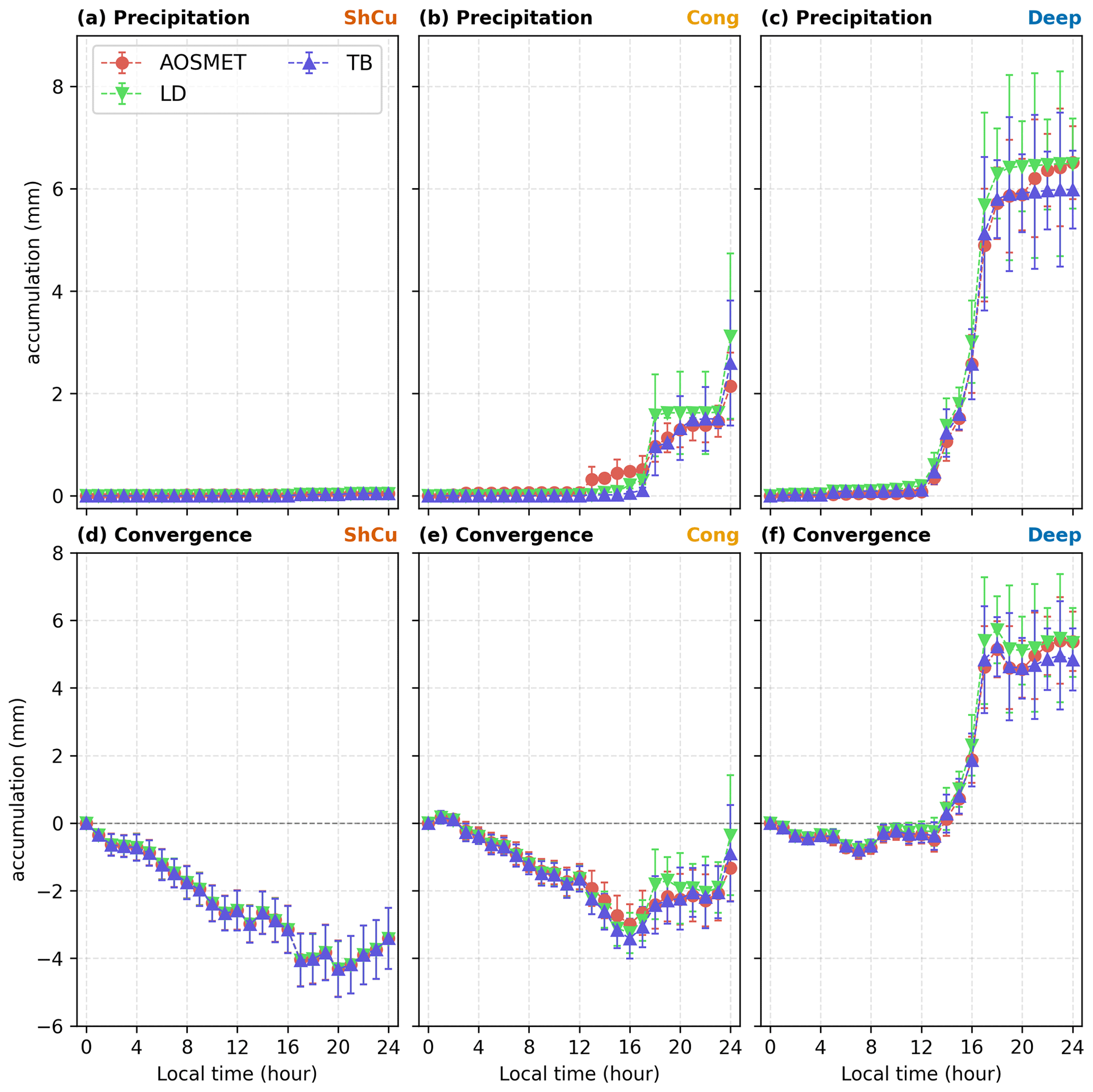
Figure A1Accumulated surface precipitation (mm) for the aerosol observing system surface data, the tipping bucket, and the laser disdrometer is shown in panels (a–c). The corresponding convergence (mm) term for each instrument is displayed in panels (d–f). (a, d) ShCu, (b, e) Cong, and (c, f) Deep regime results.
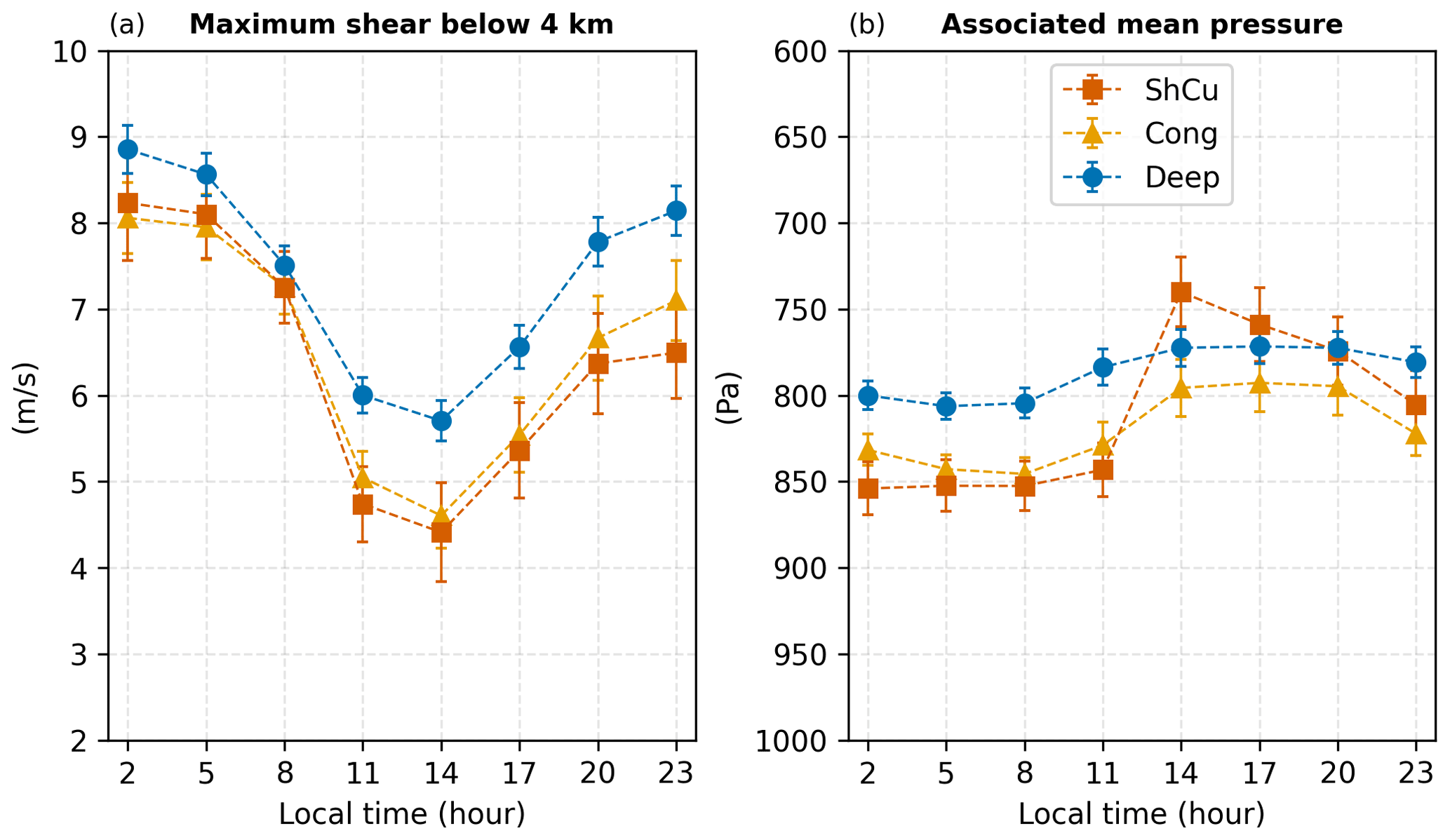
Figure A2(a) Vertical bulk wind shear from the level of maximum wind speed below 4 km and (b) the associated pressure levels.
The observational data used in this research are publicly available at https://www.arm.gov/research/campaigns/amf2014goamazon (last access: 19 November 2023; Giangrande et al., 2017; Feng and Giangrande, 2018; Schumacher and Funk, 2018a, b; ARM, 2013, 2014a, c, d, e, f, g). The variational analysis large-scale forcing data for the GoAmazon2014/5 experiment (Tang et al., 2016) are available at the ARM Archive at http://iop.archive.arm.gov/arm-iop/0eval-data/xie/scm-forcing/iop_at_mao/.
LAMV: investigation, methodology, data curation, formal analysis, visualization, and writing – original draft preparation. GT: investigation, validation, resources, and writing – review and editing. DKA: investigation and writing – review and editing. HdMJB: conceptualization, investigation, resources, supervision, and writing – review and editing.
The contact author has declared that none of the authors has any competing interests.
Publisher’s note: Copernicus Publications remains neutral with regard to jurisdictional claims made in the text, published maps, institutional affiliations, or any other geographical representation in this paper. While Copernicus Publications makes every effort to include appropriate place names, the final responsibility lies with the authors.
We acknowledge the data from the Atmospheric Radiation Measurement (ARM) Program sponsored by the US Department of Energy, Office of Science, Office of Biological and Environmental Research, Climate and Environmental Sciences Division.
Leandro Alex Moreira Viscardi was funded by the Brazilian National Council for Scientific and Technological Development (CNPq) graduate fellowship (grant no. 148652/2019-0), which supported his doctoral studies at the University of São Paulo, Brazil. Additionally, Leandro Alex Moreira Viscardi received a Coordination for the Improvement of Higher Education Personnel (CAPES) fellowship (grant no. 88887.571091/2020-00) to support 6 months of a visiting graduate student program at the University of Hawai′i at Mānoa, United States, during his doctoral journey. Henrique de Melo Jorge Barbosa was supported by the US Department of Energy, Office of Science, Biological and Environmental Research program under grant no. DE-SC-0023058.
This paper was edited by Martina Krämer and reviewed by Kyle F. Itterly and one anonymous referee.
Adams, D. K., Gutman, S. I., Holub, K. L., and Pereira, D. S.: GNSS observations of deep convective time scales in the Amazon, Geophys. Res. Lett., 40, 2818–2823, https://doi.org/10.1002/grl.50573, 2013. a, b, c, d, e, f
Adams, D. K., Barbosa, H. M. J., and Gaitán De Los Ríos, K. P.: A Spatiotemporal Water Vapor–Deep Convection Correlation Metric Derived from the Amazon Dense GNSS Meteorological Network, Mon. Weather Rev., 145, 279–288, https://doi.org/10.1175/MWR-D-16-0140.1, 2017. a, b
Adams, D. K., Fernandes, R. M. S., Holub, K. L., Gutman, S. I., Barbosa, H. M. J., Machado, L. A. T., Calhlheiros, A. J. P., Bennett, R. A., Kursinski, E. R., Sapucci, L. F., DeMets, C., Chagas, G. F. B., Arellano, A., Filizola, N., Rocha, A. A. A., Silva, R. A., Assuncao, L. M. F., Cirino, G. G., Pauliquevis, T., Portela, B. T. T., Sa, A., De Sousa, J. M., and Tanaka, L. M. S.: THE AMAZON DENSE GNSS METEOROLOGICAL NETWORK A New Approach for Examining Water Vapor and Deep Convection Interactions in the Tropics, B. Am. Meteorol. Soc., 96, 2151–2165, https://doi.org/10.1175/BAMS-D-13-00171.1, 2015. a
Anselmo, E. M., Schumacher, C., and Machado, L. A. T.: The Amazonian Low-Level Jet and Its Connection to Convective Cloud Propagation and Evolution, Mon. Weather Rev., 148, 4083–4099, https://doi.org/10.1175/MWR-D-19-0414.1, 2020. a
ARM (Atmospheric Radiation Measurement): Meteorological Measurements associated with the Aerosol Observing System (AOSMET). 2013-12-12 to 2015-12-01, ARM Mobile Facility (MAO) Manacapuru, Amazonas, Brazil, MAOS (S1), https://doi.org/10.5439/1984920, 2013. a, b, c
ARM, (Atmospheric Radiation Measurement): ARM Best Estimate Data Products (ARMBEATM). 2014-01-01 to 2015-12-31, ARM Mobile Facility (MAO) Manacapuru, Amazonas, Brazil, AMF1 (M1), https://doi.org/10.5439/1333748, 2014a. a, b
ARM (Atmospheric Radiation Measurement): Eddy Correlation Flux Measurement System (30ECOR). 2014-04-03 to 2015-12-01, ARM Mobile Facility (MAO) Manacapuru, Amazonas, Brazil, AMF1 (M1), https://doi.org/10.5439/1025039, 2014b. a
ARM (Atmospheric Radiation Measurement): Laser Disdrometer (LD). 2014-09-24 to 2015-08-13, ARM Mobile Facility (MAO) Manacapuru, Amazonas, Brazil, Supplemental Site (S10), https://doi.org/10.5439/1973058, 2014c. a, b
ARM (Atmospheric Radiation Measurement): Atmospheric Radiation Measurement (ARM) user facility. 2014. Microwave Radiometer (MWRLOS). 2014-01-06 to 2015-12-01, ARM Mobile Facility (MAO) Manacapuru, Amazonas, Brazil, AMF1 (M1), https://doi.org/10.5439/1046211, 2014d. a, b
ARM (Atmospheric Radiation Measurement): Planetary Boundary Layer Height (PBLHTSONDE1MCFARL). 2014-01-01 to 2015-12-01, ARM Mobile Facility (MAO) Manacapuru, Amazonas, Brazil, AMF1 (M1), https://doi.org/10.5439/1150253, 2014e. a, b
ARM (Atmospheric Radiation Measurement): Balloon-Borne Sounding System (SONDEWNPN). 2014-01-01 to 2015-12-01, ARM Mobile Facility (MAO) Manacapuru, Amazonas, Brazil, AMF1 (M1), https://doi.org/10.5439/1595321, 2014f. a, b
ARM (Atmospheric Radiation Measurement): Rain Gauge (RAINTB). 2014-10-14 to 2015-07-03, ARM Mobile Facility (MAO) Manacapuru, Amazonas, Brazil, Supplemental Site (S10), https://doi.org/10.5439/1224827, 2014g. a, b
Barber, K. A., Burleyson, C. D., Feng, Z., and Hagos, S. M.: The Influence of Shallow Cloud Populations on Transitions to Deep Convection in the Amazon, J. Atmos. Sci., 79, 723–743, https://doi.org/10.1175/jas-d-21-0141.1, 2022. a, b, c
Bechtold, P., Chaboureau, J.-P., Beljaars, A., Betts, A. K., Köhler, M., Miller, M., and Redelsperger, J.-L.: The simulation of the diurnal cycle of convective precipitation over land in a global model, Q. J. Roy. Meteor. Soc., 130, 3119–3137, https://doi.org/10.1256/qj.03.103, 2004. a
Betts, A. K.: Evaluation of the diurnal cycle of precipitation, surface thermodynamics, and surface fluxes in the ECMWF model using LBA data, J. Geophys. Res., 107, LBA 12-1–LBA 12-8, https://doi.org/10.1029/2001jd000427, 2002. a, b
Betts, A. K. and Jakob, C.: Study of diurnal cycle of convective precipitation over Amazonia using a single column model, J. Geophys. Res.-Atmos., 107, ACL 25-1–ACL 25-13, https://doi.org/10.1029/2002jd002264, 2002. a, b
Bretherton, C. S., Peters, M. E., and Back, L. E.: Relationships between Water Vapor Path and Precipitation over the Tropical Oceans, J. Climate, 17, 1517–1528, https://doi.org/10.1175/1520-0442(2004)017<1517:RBWVPA>2.0.CO;2, 2004. a
Cecchini, M. A., de Bruine, M., Vilà-Guerau de Arellano, J., and Artaxo, P.: Quantifying vertical wind shear effects in shallow cumulus clouds over Amazonia, Atmos. Chem. Phys., 22, 11867–11888, https://doi.org/10.5194/acp-22-11867-2022, 2022. a
Chakraborty, S., Schiro, K. A., Fu, R., and Neelin, J. D.: On the role of aerosols, humidity, and vertical wind shear in the transition of shallow-to-deep convection at the Green Ocean Amazon 2014/5 site, Atmos. Chem. Phys., 18, 11135–11148, https://doi.org/10.5194/acp-18-11135-2018, 2018. a, b, c, d
Feng, Z. and Giangrande, S.: Merged RWP-WACR-ARSCL Cloud Mask and Cloud Type, ARM [data set], https://doi.org/10.5439/1462693, 2018. a, b
Freitas, S. R., Putman, W. M., Arnold, N. P., Adams, D. K., and Grell, G. A.: Cascading Toward a Kilometer-Scale GCM: Impacts of a Scale-Aware Convection Parameterization in the Goddard Earth Observing System GCM, Geophys. Res. Lett., 47, e2020GL087682, https://doi.org/10.1029/2020gl087682, 2020. a
Ghate, V. P. and Kollias, P.: On the Controls of Daytime Precipitation in the Amazonian Dry Season, J. Hydrometeorol., 17, 3079–3097, https://doi.org/10.1175/jhm-d-16-0101.1, 2016. a, b, c, d, e, f, g, h, i, j, k, l
Giangrande, S. E., Toto, T., Jensen, M. P., Bartholomew, M. J., Feng, Z., Protat, A., Williams, C. R., Schumacher, C., and Machado, L.: Convective cloud vertical velocity and mass‐flux characteristics from radar wind profiler observations during GoAmazon2014/5, J. Geophys. Res., 121, 12891–12913, 2016. a
Giangrande, S. E., Feng, Z., Jensen, M. P., Comstock, J. M., Johnson, K. L., Toto, T., Wang, M., Burleyson, C., Bharadwaj, N., Mei, F., Machado, L. A. T., Manzi, A. O., Xie, S., Tang, S., Silva Dias, M. A. F., de Souza, R. A. F., Schumacher, C., and Martin, S. T.: Cloud characteristics, thermodynamic controls and radiative impacts during the Observations and Modeling of the Green Ocean Amazon (GoAmazon2014/5) experiment, Atmos. Chem. Phys., 17, 14519–14541, https://doi.org/10.5194/acp-17-14519-2017, 2017. a, b, c, d
Giangrande, S. E., Wang, D., and Mechem, D. B.: Cloud regimes over the Amazon Basin: perspectives from the GoAmazon2014/5 campaign, Atmos. Chem. Phys., 20, 7489–7507, https://doi.org/10.5194/acp-20-7489-2020, 2020. a, b
Grabowski, W. W., Bechtold, P., Cheng, A., Forbes, R., Halliwell, C., Khairoutdinov, M., Lang, S., Nasuno, T., Petch, J., Tao, W.-K., Wong, R., Wu, X., and Xu, K.-M.: Daytime convective development over land: A model intercomparison based on LBA observations, Q. J. Roy. Meteorol. Soc., 132, 317–344, https://doi.org/10.1256/qj.04.147, 2006. a, b
Greco, S., Swap, R., Garstang, M., Ulanski, S., Shipham, M., Harriss, R., Talbot, R., Andreae, M., and Artaxo, P.: Rainfall and surface kinematic conditions over central Amazonia during ABLE 2B, J. Geophys. Res.-Atmos., 95, 17001–17014, https://doi.org/10.1029/JD095iD10p17001, 1990. a
Gupta, A. K., Deshmukh, A., Waman, D., Patade, S., Jadav, A., Phillips, V. T. J., Bansemer, A., Martins, J. A., and Gonçalves, F. L. T.: The microphysics of the warm-rain and ice crystal processes of precipitation in simulated continental convective storms, Commun. Earth Environ., 4, 226, https://doi.org/10.1038/s43247-023-00884-5, 2023. a
Holloway, C. E. and Neelin, J. D.: Moisture Vertical Structure, Column Water Vapor, and Tropical Deep Convection, J. Atmos. Sci., 66, 1665–1683, https://doi.org/10.1175/2008JAS2806.1, 2009. a
Itterly, K. F., Taylor, P. C., Dodson, J. B., and Tawfik, A. B.: On the sensitivity of the diurnal cycle in the Amazon to convective intensity, J. Geophys. Res.-Atmos., 121, 8186–8208, https://doi.org/10.1002/2016jd025039, 2016. a, b, c, d, e
Itterly, K. F., Taylor, P. C., and Dodson, J. B.: Sensitivity of the Amazonian Convective Diurnal Cycle to Its Environment in Observations and Reanalysis, J. Geophys. Res.-Atmos., 123, 12621–12646, https://doi.org/10.1029/2018jd029251, 2018. a, b, c
Jewtoukoff, V., Plougonven, R., and Hertzog, A.: Gravity waves generated by deep tropical convection: Estimates from balloon observations and mesoscale simulations, J. Geophys. Res.-Atmos., 118, 9690–9707, https://doi.org/10.1002/jgrd.50781, 2013. a
Khairoutdinov, M. and Randall, D.: High-Resolution Simulation of Shallow-to-Deep Convection Transition over Land, J. Atmos. Sci., 63, 3421–3436, https://doi.org/10.1175/jas3810.1, 2006. a
Kuang, Z. and Bretherton, C. S.: A Mass-Flux Scheme View of a High-Resolution Simulation of a Transition from Shallow to Deep Cumulus Convection, J. Atmos. Sci., 63, 1895–1909, https://doi.org/10.1175/jas3723.1, 2006. a
Machado, L., Laurent, H., Dessay, N., and Miranda, I.: Seasonal and diurnal variability of convection over the Amazonia: A comparison of different vegetation types and large scale forcing, Theor. Appl. Climatol., 78, 61–77, https://doi.org/10.1007/s00704-004-0044-9, 2004. a
Machado, L. A. T.: Diurnal march of the convection observed during TRMM-WETAMC/LBA, J. Geophys. Res., 107, LBA 31-1–LBA 31-15, https://doi.org/10.1029/2001jd000338, 2002. a, b
Maher, P., Vallis, G. K., Sherwood, S. C., Webb, M. J., and Sansom, P. G.: The Impact of Parameterized Convection on Climatological Precipitation in Atmospheric Global Climate Models, Geophys. Res. Lett., 45, 3728–3736, https://doi.org/10.1002/2017gl076826, 2018. a
Mapes, B. and Neale, R.: Parameterizing Convective Organization to Escape the Entrainment Dilemma, J. Adv. Model. Earth Sy., 3, M06004, https://doi.org/10.1029/2011MS000042, 2011. a
Mapes, B., Tulich, S., Lin, J., and Zuidema, P.: The mesoscale convection life cycle: Building block or prototype for large-scale tropical waves?, Dynam. Atmos. Oceans, 42, 3–29, https://doi.org/10.1016/j.dynatmoce.2006.03.003, 2006. a
Marengo, J. A., Alves, L. M., Soares, W. R., Rodriguez, D. A., Camargo, H., Riveros, M. P., and Pabló, A. D.: Two Contrasting Severe Seasonal Extremes in Tropical South America in 2012: Flood in Amazonia and Drought in Northeast Brazil, J. Climate, 26, 9137–9154, https://doi.org/10.1175/jcli-d-12-00642.1, 2013. a
Martin, S. T., Artaxo, P., Machado, L. A. T., Manzi, A. O., Souza, R. A. F., Schumacher, C., Wang, J., Andreae, M. O., Barbosa, H. M. J., Fan, J., Fisch, G., Goldstein, A. H., Guenther, A., Jimenez, J. L., Pöschl, U., Silva Dias, M. A., Smith, J. N., and Wendisch, M.: Introduction: Observations and Modeling of the Green Ocean Amazon (GoAmazon2014/5), Atmos. Chem. Phys., 16, 4785–4797, https://doi.org/10.5194/acp-16-4785-2016, 2016. a, b, c
Martin, S. T., Artaxo, P., Machado, L., Manzi, A. O., Souza, R. A. F., Schumacher, C., Wang, J., Biscaro, T., Brito, J., Calheiros, A., Jardine, K., Medeiros, A., Portela, B., de Sá, S. S., Adachi, K., Aiken, A. C., Albrecht, R., Alexander, L., Andreae, M. O., Barbosa, H. M. J., Buseck, P., Chand, D., Comstock, J. M., Day, D. A., Dubey, M., Fan, J., Fast, J., Fisch, G., Fortner, E., Giangrande, S., Gilles, M., Goldstein, A. H., Guenther, A., Hubbe, J., Jensen, M., Jimenez, J. L., Keutsch, F. N., Kim, S., Kuang, C., Laskin, A., McKinney, K., Mei, F., Miller, M., Nascimento, R., Pauliquevis, T., Pekour, M., Peres, J., Petäjä, T., Pöhlker, C., Pöschl, U., Rizzo, L., Schmid, B., Shilling, J. E., Dias, M. A. S., Smith, J. N., Tomlinson, J. M., Tóta, J., and Wendisch, M.: The Green Ocean Amazon Experiment (GoAmazon2014/5) Observes Pollution Affecting Gases, Aerosols, Clouds, and Rainfall over the Rain Forest, B. Am. Meteorol. Soc., 98, 981–997, https://doi.org/10.1175/bams-d-15-00221.1, 2017. a, b
Morrison, H., Peters, J. M., Chandrakar, K. K., and Sherwood, S. C.: Influences of Environmental Relative Humidity and Horizontal Scale of Subcloud Ascent on Deep Convective Initiation, J. Atmos. Sci., 79, 337–359, https://doi.org/10.1175/jas-d-21-0056.1, 2022. a
Schiro, K. A., Neelin, J. D., Adams, D. K., and Lintner, B. R.: Deep Convection and Column Water Vapor over Tropical Land versus Tropical Ocean: A Comparison between the Amazon and the Tropical Western Pacific, J. Atmos. Sci., 73, 4043–4063, https://doi.org/10.1175/jas-d-16-0119.1, 2016. a, b, c
Schiro, K. A., Ahmed, F., Giangrande, S. E., and Neelin, J. D.: GoAmazon2014/5 campaign points to deep-inflow approach to deep convection across scales, P. Natl. Acad. Sci. USA, 115, 4577–4582, https://doi.org/10.1073/pnas.1719842115, 2018. a, b, c, d
Schlemmer, L. and Hohenegger, C.: Modifications of the atmospheric moisture field as a result of cold-pool dynamics, Q. J. Roy. Meteor. Soc., 142, 30–42, https://doi.org/10.1002/qj.2625, 2015. a
Schumacher, C. and Funk, A.: GoAmazon2014/5 Three-dimensional Gridded S-band Reflectivity and Radial Velocity from the SIPAM Manaus S-band Radar, ARM-IOP, https://doi.org/10.5439/1459573, 2018a. a, b, c
Schumacher, C. and Funk, A.: GoAmazon2014/5 Rain Rates from the SIPAM Manaus S-band Radar, ARM-IOP, https://doi.org/10.5439/1459578, 2018b. a, b, c
Sherwood, S. C., Bony, S., and Dufresne, J.-L.: Spread in model climate sensitivity traced to atmospheric convective mixing, Nature, 505, 37–42, https://doi.org/10.1038/nature12829, 2014. a
Silva Dias, M. A. F.: Cloud and rain processes in a biosphere-atmosphere interaction context in the Amazon Region, J. Geophys. Res., 107, LBA 39-1–LBA 39-18, https://doi.org/10.1029/2001jd000335, 2002. a
Stevens, B. and Bony, S.: What Are Climate Models Missing?, Science, 340, 1053–1054, https://doi.org/10.1126/science.1237554, 2013. a
Stull, R.: Practical Meteorology: An Algebra-Based Survey of Atmospheric Science – version 1.02b, Univ. of British Columbia, 940 pp., ISBN 978-0-88865-283-6, 2017. a
Tang, S., Xie, S., Zhang, Y., Zhang, M., Schumacher, C., Upton, H., Jensen, M. P., Johnson, K. L., Wang, M., Ahlgrimm, M., Feng, Z., Minnis, P., and Thieman, M.: Large-scale vertical velocity, diabatic heating and drying profiles associated with seasonal and diurnal variations of convective systems observed in the GoAmazon2014/5 experiment, Atmos. Chem. Phys., 16, 14249–14264, https://doi.org/10.5194/acp-16-14249-2016, 2016 (data available at: http://iop.archive.arm.gov/arm-iop/0eval-data/xie/scm-forcing/iop_at_mao/, last access: 19 November 2023). a, b, c
Tian, Y., Zhang, Y., Klein, S. A., and Schumacher, C.: Interpreting the diurnal cycle of clouds and precipitation in the ARM GoAmazon observations: Shallow to deep convection transition, J. Geophys. Res.-Atmos., 126, e2020JD033766, https://doi.org/10.1029/2020JD033766, 2021. a, b, c, d, e, f, g, h, i, j, k
Tota, J., Fisch, G., Oliveira, P., Fuentes, J., and Siegler, J.: Análise da variabilidade diária da precipitação em área de pastagem para a época chuvosa de 1999 – projeto TRMM/LBA, Acta Amazon., 30, 629–629, https://doi.org/10.1590/1809-43922000304639, 2000. a, b
Waite, M. L. and Khouider, B.: The Deepening of Tropical Convection by Congestus Preconditioning, J. Atmos. Sci., 67, 2601–2615, https://doi.org/10.1175/2010jas3357.1, 2010. a
Wu, C.-M., Stevens, B., and Arakawa, A.: What Controls the Transition from Shallow to Deep Convection?, J. Atmos. Sci., 66, 1793–1806, https://doi.org/10.1175/2008jas2945.1, 2009. a
Zhuang, Y., Fu, R., Marengo, J. A., and Wang, H.: Seasonal variation of shallow-to-deep convection transition and its link to the environmental conditions over the Central Amazon, J. Geophys. Res.-Atmos., 122, 2649–2666, https://doi.org/10.1002/2016jd025993, 2017. a, b, c, d, e, f, g, h, i, j, k, l, m, n, o, p, q, r
- Abstract
- Introduction
- Data and methods
- Cloud and precipitation properties
- Environmental conditions
- Conditionally averaged precipitation
- Discussion
- Conclusions
- Appendix A: Additional material
- Data availability
- Author contributions
- Competing interests
- Disclaimer
- Acknowledgements
- Financial support
- Review statement
- References