A model study investigating the sensitivity of aerosol forcing to the volatilities of semi-volatile organic compounds

Secondary organic aerosol (SOA) constitutes an important component of atmospheric particulate matter, with a substantial influence on air quality, human health and the global climate. The volatility basis set (VBS) framework has provided a valuable tool for better simulating the formation and evolution of SOA where SOA precursors are grouped by their volatility. This is done in order to avoid the computational cost of simulating possibly hundreds of atmospheric organic species involved in SOA formation. The accuracy of this framework relies upon the accuracy of the volatility distribution of the oxidation products of volatile organic compounds (VOCs) used to represent SOA formation. However, the volatility distribution of SOA-forming vapours remains inadequately constrained within global climate models, leading to uncertainties in the predicted aerosol mass loads and climate impacts. This study presents the results from simulations using a process-scale particle growth model and a global climate model, illustrating how uncertainties in the volatility distribution of biogenic SOA precursor gases affect the simulated cloud condensation nuclei (CCN). We primarily focused on the volatility of oxidation products derived from monoterpenes as they represent the dominant class of VOCs emitted by boreal trees. Our findings reveal that the particle growth rate and their survival to CCN sizes, as simulated by the process-scale model, are highly sensitive to uncertainties in the volatilities of condensing organic vapours. Interestingly, we note that this high sensitivity is less pronounce in global-scale model simulations as the CCN concentration and cloud droplet number concentration (CDNC) simulated in the global model remain insensitive to a 1-order-of-magnitude shift in the volatility distribution of organics. However, a notable difference arises in the SOA mass concentration as a result of volatility shifts in the global model. Specifically, a 1-order-of-magnitude decrease in volatility corresponds to an approximate 13 % increase in SOA mass concentration, while a 1-order-of-magnitude increase results in a 9 % decrease in SOA mass concentration over the boreal region. SOA mass and CCN concentrations are found to be more sensitive to the uncertainties associated with the volatility of semi-volatile compounds, with saturation concentrations of 10⁻¹ µg m⁻³ or higher, than the low-volatility compounds. This finding underscores the importance of having a higher resolution in the semi-volatile bins, especially in global models, to accurately capture SOA formation. Furthermore, the study highlights the importance of a better representation of saturation concentration values for volatility bins when employing a reduced number of bins in a global-scale model. A comparative analysis between a finely resolved nine-bin VBS setup and a simpler three-bin VBS setup highlights the significance of these choices. The study also indicates that radiative forcing attributed to changes in SOA over the boreal forest region is notably more sensitive to the volatility distribution of semi-volatile compounds than low-volatility compounds. In the three-bin VBS setup, a 10-fold decrease in the volatility of the highest-volatility bin results in a shortwave instantaneous radiative forcing (IRF_ari) of −0.2 ± 0.10 W m⁻² and an effective radiative forcing (ERF) of +0.8 ± 2.24 W m⁻², while a 10-fold increase in volatility leads to an IRF_ari of +0.05 ± 0.04 W m⁻² and an ERF of +0.45 ± 2.3 W m⁻² over the boreal forest region. These findings underscore the critical need for a more accurate representation of semi-volatile compounds within global-scale models to effectively capture the aerosol loads and the subsequent climate effects.

1 Introduction

Organic aerosol (OA) plays a critical role in atmospheric chemistry, comprising a significant fraction of sub-micrometre atmospheric aerosols (Jimenez et al., 2009). These atmospheric aerosol make up 20 %–90 % of the total submicron aerosol loading (Jimenez et al., 2009; Hallquist et al., 2009), and they are crucial for both human health and the climate. OA includes primary organic aerosol (POA) and secondary organic aerosol (SOA), both of which are composed of a mixture of organic chemical species. POA is directly emitted into the atmosphere from a variety of sources, such as vegetation, biomass burning and fossil fuel combustion (Spracklen et al., 2011). In contrast, SOA is formed in the atmosphere by the gas-phase oxidation of organic compounds to form products that subsequently condense into the aerosol phase (Kroll and Seinfeld, 2008). This condensation process largely depends on the saturation vapour concentration (C_sat) of the oxidized products. The formation of SOA is driven by the oxidation of a variety of volatile organic compounds (VOCs) or semi-volatile organic compounds (SVOCs) present in the atmosphere through reactions with oxidants such as hydroxyl radicals (OH), ozone (O₃) and nitrate radicals (NO₃) (Ng et al., 2017). The oxidation of these organic compounds can then lead to the formation of an extensive range of low-volatility and semi-volatile products that can then condense into the particle phase (Hallquist et al., 2009). Terpenes (e.g. α-pinene and β-pinene) and isoprene are dominant sources of biogenic VOCs globally, while alkanes and aromatics (e.g. toluene and xylene) are the major anthropogenic VOCs (Ziemann and Atkinson, 2012). In the boreal ecosystem, monoterpenes account for the majority of VOC emissions, which yield a significant amount of global SOA, comprising more than half of the total biogenic SOA (Yu et al., 2021).

SOA, especially that of biogenic origin, plays a significant role in Earth's climate, primarily through its influence on aerosol–cloud interactions and aerosol–radiation interactions (Scott et al., 2014; Yli-Juuti et al., 2021; Petäjä et al., 2022). In particular, the effect of SOA on clouds is mainly determined by the particles that grow to cloud condensation nuclei (CCN) sizes (typically 30 to 100 nm), primarily through the process of condensation (Pierce and Adams, 2007; Pierce et al., 2012). In addition to its effect on cloud properties, SOA can also affect climate directly by affecting the radiative transfer of solar radiation in the atmosphere. SOA significantly scatters solar radiation, which can lead to a cooling effect on the Earth's surface (Shrivastava et al., 2017).

Even though there have been substantial improvements in understanding the properties and formation mechanisms of biogenic SOA, their representation in the current climate models is still poorly constrained (Hodzic et al., 2016; Shrivastava et al., 2017; Tsigaridis and Kanakidou, 2018; Liu et al., 2021). One potential source of these uncertainties is associated with the complex and highly variable composition of SOA and its precursors (Zhu et al., 2017), which is influenced by a variety of different VOCs and their multiple oxidation pathways (Donahue et al., 2012). Although certain climate models have made progress in simulating the formation of SOA, there are still uncertainties, particularly regarding aspects related to the representation of organic vapours. Given the wide spectrum of SOA precursor species, their concentrations and their compositions, several of the current climate models (for example, ECHAM-SALSA (European Centre Hamburg Model – Sectional Aerosol module for Large Scale Applications) (Mielonen et al., 2018), CESM2 (Community Earth System Model 2) (Tilmes et al., 2019), GEOS-CHEM (Goddard Earth Observing System – Atmospheric Chemistry) (Fritz et al., 2022) and GFDL AM (Geophysical Fluid Dynamics Laboratory's Atmosphere Model) (Zheng et al., 2023)) use the volatility basis set (VBS) approach to represent SOA and to simulate the formation of SOA in the atmosphere. The VBS framework provides a systematic and computationally efficient way to represent the multitude of organic compounds and their varying volatilities, which determine how they partition between the gas and particle phases in the atmosphere (Donahue et al., 2006). In the VBS approach, SOA is treated as a mixture of organic compounds of varying volatility that are distributed among a set of discrete volatility bins based on their vapour pressure (Donahue et al., 2011). The VBS framework aims to simplify the complex and often poorly understood processes involved in SOA formation. This simplification is achieved by combining compounds into groups based on their volatility, reducing the complexity of chemical processes involved in the formation and ageing of SOA (Donahue et al., 2006). The VBS approach has been shown to be effective at simulating the concentration and composition of SOA in the atmosphere and can be used to study the impacts of SOA on air quality and the climate (Tsimpidi et al., 2010; Jathar et al., 2017; Jiang et al., 2019).

Monoterpenes dominate the VOC emissions in boreal forested areas, covering 29 % of forested land areas, thereby making this region a significant source of biogenic SOA (Rinne et al., 2009; Kayes and Mallik, 2020). Hence, the significance of monoterpenes and their oxidation products in understanding global natural background aerosol burdens is evident. Several studies have demonstrated the importance of the oxidation products of monoterpenes and their vapour pressures in new particle formation and growth at a process level (e.g. Ehn et al., 2014; Tröstl et al., 2016; Kirkby et al., 2016; Yli-Juuti et al., 2017; Lehtipalo et al., 2018; Roldin et al., 2019; Mohr et al., 2019). However, the sensitivity of global-model outputs (CCN concentrations, cloud droplet number concentration (CDNC) and radiative forcing) to uncertainties in the volatilities of compounds or the resolution (i.e. number of bins) in VBS representing monoterpene oxidation products remains inadequately studied.

In this study, we used a process-scale growth model and a global aerosol–climate model to investigate the sensitivity of the volatility distribution to SOA formation and cloud properties. The process model focused on examining the sensitivity of particle growth rate and their survival across CCN size ranges to uncertainties in the volatilities of organic vapours at a process scale. One motivation for this study was to examine how process model results, which only take into account microphysical processes, translate to the global scale, which also includes several processes that can buffer the changes SOA makes to the aerosol population. To understand how these sensitivities at the process scale manifest at a global scale, we utilized the global aerosol–climate model ECHAM-HAMMOZ coupled with the aerosol microphysical model SALSA, which is the Sectional Aerosol module for Large Scale Applications (Kokkola et al., 2018; Holopainen et al., 2020, 2022). This allowed us to study how sensitive the simulated SOA formation is to the assumptions regarding the volatility distributions of biogenic SOA precursors, specifically monoterpenes, over the boreal region. We also investigated how this sensitivity translates to sensitivities in simulated cloud properties, as well as in the radiative properties of the atmosphere. To study the sensitivity of SOA mass and CCN concentrations to uncertainties in the volatility distribution, we shifted the volatility of monoterpene oxidation products across all VBS bins by 1 order of magnitude. Additionally, we shifted the volatilities of individual VBS bins by 1 order of magnitude to assess the effect of uncertainties in the volatility of each VBS bin. To investigate the sensitivity of model outputs to VBS resolution, we tested two setups using the VBS approach. The first setup describes the volatility of SOA precursors by grouping them into nine volatility classes (hereafter referred to as the nine-bin VBS setup), while the second one groups them into three volatility classes (hereafter referred to as the three-bin VBS setup). From these simulations, we analysed how the assumptions and changes in the volatility distribution affect SOA mass, CCN and cloud properties. Overall, this study aims to provide insights into the importance of accurately representing the volatility distribution of organic aerosols when modelling the formation of SOA in a global climate model.

2 Methods

2.1 Particle growth model

We simulated the growth of nucleation-mode particles and their survival to CCN size on the process scale with the model for coagulation losses in nanoparticle growth (MCOLNAG). MCOLNAG specifically focuses on understanding the effect of uncertainties in volatility distribution on particle growth and CCN concentration. The model simulates the growth of a monodisperse nucleation-mode particle population due to condensation of vapours and the decrease in the nucleation-mode particle number concentration due to coagulation. Condensation growth for compounds other than water is calculated based on a transition regime mass flux equation including the effects of particle motion and vapour molecule volume, which are influential at small sizes (Fuchs and Sutugin, 1970; Lehtinen and Kulmala, 2003). Water uptake by growing particles is calculated by assuming constant instantaneous equilibration between the gas and particle phases. The particle phase is assumed to form an ideal solution, behaving in a liquid-like manner, and no particle-phase chemical reactions are included. Decreases in nucleation-mode particle concentration due to coagulation scavenging to Aitken and accumulation modes and self-coagulation within the nucleation mode are included. Aitken- and accumulation-mode particle diameters and number concentrations are set to be constant. Self-coagulation decreases the nucleation-mode number concentration, but its impact on particle size is ignored; i.e. the nucleation-mode particles grow in the model by means of condensation only.

In this study, condensing vapours included the organic vapours presented with a nine-bin VBS and water. Concentrations of each bin were defined by setting the total concentration of organic vapours and multiplying that with the stoichiometric coefficient of the respective bin (see Sect. 2.3 for stoichiometric coefficients). Particle number concentrations and diameters of the Aitken and accumulation modes, as well as the initial number concentration of the nucleation mode, were set to spring-time median values at the boreal-forest measurement station Hyytiälä, as reported by Leinonen et al. (2022). Number concentrations were 1161 and 321 cm⁻³ and diameters were 53 nm and 170 nm for the Aitken and accumulation modes, respectively. The initial number concentration of the nucleation mode was 539 cm⁻³, and the initial diameter of the nucleation-mode particles was 3 nm. The molar mass of the organic compounds was 200 gm⁻¹; the gas-phase diffusion coefficient at 273.15 K was 5 × 10⁻⁶ m²s⁻¹, from which the value at the set temperature was calculated; the mass accommodation coefficient was 1; the particle density was 1200 kgm⁻³; and the surface tension of the particle was 30 mNm⁻¹. The simulations were performed at 298 K.

2.2 Global aerosol–climate model ECHAM-SALSA

We used the global aerosol–climate model ECHAM-HAMMOZ (ECHAM6.3-HAM2.3) (Schultz et al., 2018) to study the sensitivity of SOA formation and cloud properties to changes in the volatility distribution of organics. ECHAM-HAMMOZ consists of the atmospheric general circulation model ECHAM6, which solves the equations of motion and continuity for the atmosphere using the spectral method. In this study, all simulations utilized the T63 spectral truncation for the horizontal resolution, which corresponds to a grid spacing of roughly 1.9° × 1.9°, and 47 hybrid sigma-pressure levels for the vertical resolution.

HAM (Hamburg Aerosol Module) (Kokkola et al., 2018; Tegen et al., 2019) in ECHAM-HAM simulates the life cycle of aerosols in the atmosphere, including their formation, growth and removal processes. HAM includes a comprehensive treatment of aerosol microphysics, including the formation of SOA from gas-phase precursors, the growth of particles through coagulation, emissions of gases and aerosol, the removal of particles by dry and wet deposition, aerosol–radiation interactions, and aerosol–cloud interactions.

HAM offers two different options for modelling aerosol microphysics. One of the options is the modal aerosol module, called M7, which is designed to simulate the number and mass concentrations of different aerosol modes based on their size and composition (Vignati et al., 2004; Stier et al., 2005). The other option is called the Sectional Aerosol module for Large Scale Applications (SALSA) (Kokkola et al., 2018), which uses a sectional approach to model aerosol microphysics. In this study, ECHAM-HAMMOZ is coupled with SALSA (Kokkola et al., 2018), employing a detailed sectional representation of aerosol microphysics. SALSA uses several discrete size classes to represent the aerosol size distribution, which is described more in Sect. 2.2.1. Out of the two options, only SALSA includes the VBS approach for describing SOA formation.

2.2.1 SALSA

SALSA is an advanced aerosol microphysical model that simulates the size distribution and chemical composition of atmospheric aerosols. SALSA uses a sectional approach where the aerosol size distribution is divided into 10 size classes in size space, ranging from 3 nm to 10 µm. For particles larger than 50 nm, the model includes parallel externally mixed size classes (Kokkola et al., 2018). SALSA includes a comprehensive treatment of aerosol microphysics, including nucleation, condensation/evaporation, coagulation, and hydration. The SALSA-simulated aerosol is also coupled to aerosol–cloud interactions, as well as radiation, allowing for investigations of the impacts of aerosols on the Earth's radiative budget and, thus, the climate. Cloud droplet activation is solved using the parameterization by Abdul-Razzak and Ghan (2002), which calculates the fraction of activated particles in each size class. SALSA treats the following chemical species: sulfate, organic carbon, black carbon, sea salt and mineral dust. A detailed description of the model is given by Kokkola et al. (2018). However, recently, SALSA has undergone further advancements to enhance its wet-scavenging scheme, as introduced by Holopainen et al. (2020). SALSA has been used in numerous studies at different spatial scales (e.g. Bergman et al., 2011; Andersson et al., 2015; Tonttila et al., 2017; Kühn et al., 2020; Miinalainen et al., 2021; Holopainen et al., 2022) to investigate the behaviour of atmospheric aerosols and their impacts on the climate.

2.2.2 SOA formation routine of SALSA

SALSA includes a comprehensive SOA parameterization based on the VBS framework (Stadtler et al., 2018; Mielonen et al., 2018). In this study, we have set up the VBS approach so that it categorizes VBS compounds into either nine or three different volatility bins. SOA is composed of both anthropogenic and biogenic VOC sources. SOA formation is represented by the partitioning of the oxidized organic compounds between the gas and particle phases based on their volatility. To estimate the partitioning of VOC oxidation products between the gas and particle phases, the analytical predictor of condensation (APC) method, developed by Jacobson (2005), is used. The APC method calculates the partitioning of VBS species by solving the condensation equation,

$$\begin{array}{}\text{(1)}& {\displaystyle \frac{\mathrm{d}{C}_{\text{org},i}}{\mathrm{d}t}}=k_{\mathrm{m},i}(C_{\text{org},i,\text{surf}}-C_{\text{org},\text{gas}}),\end{array}$$

numerically. This enables the estimation of the non-equilibrium partitioning of each organic compound “org” between the gas phase and each aerosol size class i and, thus, their contribution to SOA formation. To avoid any oscillatory behaviours in condensation, we solve the condensation equations using five time steps to solve the condensation over one atmospheric model time step, with the condensation solver time step length increasing logarithmically. Equation (1) describes the rate of change of the gas-phase concentration of the organic compound, represented by C_org,i, with time (dt) and is a function of the mass transfer coefficient k_m,i, the surface equilibrium concentration of the organic compound in the particle phase $C_{\text{org},i,\text{surf}}$ and the gas-phase concentration of the organic compound. The calculation of the saturation concentration at the surface of a droplet is determined using

$$\begin{array}{}\text{(2)}& C_{\text{org},i,\text{surf}}=S^{\prime }{C}_{\text{org},i,\text{surf}}=S_i^{\prime }{x}_{\text{org},i}{C}_{\text{org},\text{sat}}.\end{array}$$

In Eq. (2), $S_i^{\prime }$ represents the Kelvin effect, x_org,i represents the mole fraction of the organic compound, and C_org,sat represents the saturation concentration of the condensing compound. In these equations, concentrations are expressed as mole concentrations (mol m⁻³), which are derived from mass-concentration-based values. The method assumes that the behaviour of the condensing organic compounds in the condensed phase is ideal (Kokkola et al., 2014).

2.3 Formulation of the volatility distribution

ECHAM-SALSA normally uses a three-bin VBS setup for monoterpene oxidation products with C_sat values of 0, 1 and 10 µg m⁻³ and different stoichiometric parameters for low- and high-NO_x conditions based on Pathak et al. (2007). In order to analyse the sensitivity of SOA formation to volatility distribution, we needed to implement a VBS parameterization for monoterpene oxidation products with more volatility bins than in the default model setup. Hence, we constructed the volatility distribution of SOA precursors based on previous studies conducted by Tröstl et al. (2016) and Hunter et al. (2017). Tröstl et al. (2016) conducted a chamber experiment to determine the gas-phase volatility distribution of α-pinene oxidation products (Fig. 5b, Extended Data, in Tröstl et al., 2016). Extremely low-volatility organic compound (ELVOC) concentrations were measured using a nitrate chemical ionization mass spectrometer (CIMS), while LVOC and SVOC concentrations were estimated based on the growth rates of nanoparticles. Hunter et al. (2017) measured organic concentrations in the particle and gas phases during summertime in a Ponderosa pine forest using five mass spectrometers. Here, we used their reported campaign average volatility distribution (Hunter et al., 2017) but included only the gas-phase data and excluded the fraction referring to the particle phase. However, the results from Tröstl et al. (2016) for the upper end of the LVOC range and for SVOCs are uncertain due to the lower sensitivity of particle growth to these compounds, and they omitted saturation concentrations higher than 100 µg m⁻³. In contrast, Hunter et al. (2017) did not detect gas-phase ELVOCs, even though their existence has been established in α-pinene laboratory systems and boreal forest. This suggests that their array of mass spectrometers had some deficiencies in detecting organic compounds at the lower end of volatilities. Therefore, the volatility distribution for this study was constructed by combining the volatility distributions from both Hunter et al. (2017) and Tröstl et al. (2016). Hunter et al. (2017) report volatilities at 298 K as the reference temperature for C_sat, while the experiments of Tröstl et al. (2016) were performed at 278 K. In order to combine the two volatility distributions, the volatility distribution from Tröstl et al. (2016) was converted to 298 K assuming a vaporization enthalpy (ΔH_vap) of 30 kJmol⁻¹ (Farina et al., 2010). First, a logarithmic uniform distribution of compounds within each VBS bin was assumed (i.e. between 10^n−0.5–10^n+0.5 µg m⁻³ for the bin C_sat = 10ⁿ µg m⁻³), and the concentration of each bin was divided into 100 logarithmically uniformly distributed sub-bins. Third, the sub-bins were redistributed into traditional VBS bins at 298 K, with C_sat values of full orders of magnitude using the bin limits of 10^n−0.5–10^n+0.5 µg m⁻³ or the bin with C_sat = 10ⁿ µg m⁻³.

The two volatility distributions were combined by assuming that both distributions included all the compounds that belong to the bin C_sat = 10⁻¹ µg m⁻³ at 298 K. First, the concentrations in each bin in both volatility distributions were normalized to the concentration in bin C_sat = 10⁻¹ µg m⁻³. Then the combined volatility distribution was constructed by selecting the volatility bins C_sat ≤ 10⁻¹ µg m⁻³ from Tröstl et al. (2016) and the bins 10⁻¹ µg m⁻³ < C_sat < 10¹ µg m⁻³ from Hunter et al. (2017). Finally, the total concentration in the constructed volatility distribution was normalized to 1, which provided a normalized distribution to use as a starting point to generate volatility basis sets with different numbers of bins.

In order to reduce the computational costs, the number of volatility bins was reduced by combining the bins C_sat ≤ 10⁻⁵ µg m⁻³ into one non-volatile bin (C_sat = 0). This is a reasonable simplification since the growth process is insensitive to the saturation concentration of such extremely low-volatility compounds (Kokkola et al., 2014). This resulted in a nine-bin VBS with one non-volatile bin and eight bins where 10⁻⁴ µg m⁻³ ≤ C_sat ≤ 10³ µg m⁻³. The stoichiometric coefficients for each volatility bin were calculated by multiplying the sum of the stoichiometric coefficients by the normalized concentration in the respective bin. The C_sat values and the corresponding stoichiometric coefficients for the nine-bin VBS setup are given in Table 1.

Table 1 Overview of saturation concentrations and stoichiometric coefficients used for nine-bin and three-bin VBS setups.

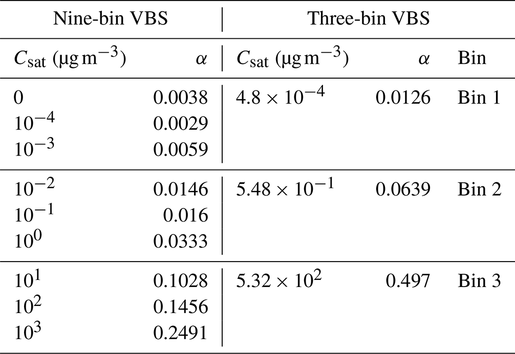
The described nine-bin VBS setup is computationally very expensive to use in a global sectional aerosol model framework such as SALSA. This is why the VBS setup of several global models, for instance, WRF-CHEM (Reyes-Villegas et al., 2022), CESM2 (Tilmes et al., 2019) and the previous version of ECHAM-SALSA (Mielonen et al., 2018), have simpler VBS representations. However, the implications of such a simplification have not previously been studied in a global-model framework. To compare the impact of the number of volatility bins on the SOA formation and the climate, a three-bin VBS setup was developed based on the already formulated nine-bin VBS setup. The three-bin VBS setup lumped together the adjacent bins from the nine-bin VBS setup to form three bins. Bin 1 consisted of the three adjacent bins with C_sat values of 0, 10⁻⁴ and 10⁻³ µg m⁻³; bin 2 included C_sat values of 10⁻², 10⁻¹ and 10⁰ µg m⁻³; and bin 3 comprised C_sat values of 10¹, 10² and 10³ µg m⁻³. The stoichiometric coefficients for the three-bin VBS setup were obtained by summing the stoichiometric coefficients of the three bins considered from the nine-bin VBS setup. Consequently, the total production of condensable organics resulting from the oxidation of monoterpene remained unchanged between the nine-bin VBS setup and the three-bin VBS setup. In the three-bin VBS setup, we calculated the saturation concentration for each bin as the concentration-weighted arithmetic average of the three lumped bins from the nine-bin VBS setup. The C_sat values and the corresponding stoichiometric coefficients for the three-bin VBS setup are given in Table 1.

2.4 ECHAM-SALSA simulations

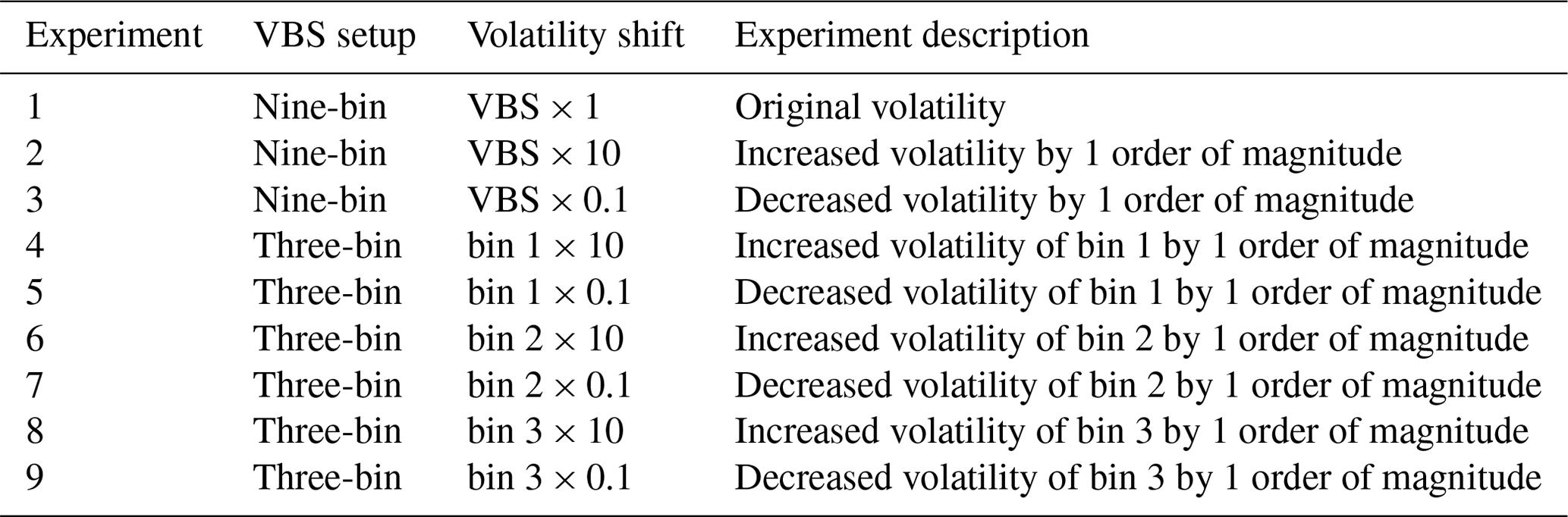
A series of simulations were conducted using the global aerosol–climate model ECHAM-SALSA to investigate the effect of shifts in the volatility of monoterpene oxidation products on aerosol properties and radiative forcing. Two different VBS setups were used, namely a nine-bin VBS setup and a three-bin VBS setup, to evaluate the sensitivity of the model to the number of volatility bins. Three different simulations were performed using the nine-bin VBS setup to assess the impact of uncertainties in the volatility distribution by shifting the volatility of monoterpene oxidation products by 1 order of magnitude. The simulations were conducted for the original volatility (VBS × 1), increased volatility (VBS × 10) and decreased volatility (VBS × 0.1). Another set of six different simulations were carried out using the three-bin VBS setup to study the effect of uncertainties associated with the volatilities of individual VBS bins, where the volatility of each VBS bin was shifted by 1 order of magnitude. A summary of all the simulations is given in Table 2. We studied the sensitivity of SOA mass, CCN and radiative forcing to the volatility assumptions across all simulations. The number concentration of particles greater than 100 nm (N100) in diameter was used as a proxy for the CCN concentration (Clarke and Kapustin, 2010). This study focused solely on the shift in the oxidation products of monoterpenes as these are the most abundant VOCs emitted by the boreal trees (Rinne et al., 2009). Furthermore, the highest emissions of monoterpene from the boreal trees generally occur during the summer season (Vanhatalo et al., 2020); therefore, we specifically studied the summer season (June, July and August) of the simulation year 2010. Consequently, all the findings and results from this study are specific to the boreal-forest region in the Northern Hemisphere, where the summer season is characterized by intense monoterpene emissions and their subsequent impact on aerosol dynamics.

Table 2 Summary of experiments.

All the simulations employed emission data from the Community Emissions Data System (CEDS) for the anthropogenic emissions (Hoesly et al., 2018). In addition, we used the biomass burning emissions from the Biomass Burning for Model Intercomparison Projects (BB4MIPs) inventory (Van Marle et al., 2017). The simulations were designed to allow the model atmospheric circulation to evolve freely while using fixed sea surface temperature (SST) and sea ice cover (SIC). Monthly mean climatologies from the Atmospheric Model Intercomparison Project (AMIP) provided the SST and SIC values (Taylor et al., 2012). To evaluate the impact of different assumed volatility distributions on the Earth's simulated radiation balance, we calculated the shortwave effective radiative forcing (ERF) suggested by Forster et al. (2016), which is the difference in the net top-of-atmosphere (TOA) radiative fluxes between simulations with different volatility distributions and the original volatility distribution. Furthermore, we calculated the shortwave instantaneous radiative forcing due to aerosol–radiation interactions (IRF_ari) in ECHAM-SALSA by performing a double call to the radiation scheme with and without the aerosol perturbation, as described in Collins et al. (2006). IRF_ari differentiates the direct radiative effect of aerosols from the impact of aerosols on circulation and cloudiness, which corresponds to the difference in net TOA radiative flux solely due to the absorption and scattering of aerosols without any contributions from adjustments. Additionally, we calculated the 1-sigma standard deviation across different grid cells over the boreal forests, indicating the variability within the boreal-forest regions.

3 Results

3.1 Particle growth model MCOLNAG

Figure 1 shows the particle growth simulated with MCOLNAG with the base-case VBS and with the volatilities shifted to higher or lower values by 1 order of magnitude, as well as the fraction of nucleation-mode particles that survive from the initial 3 nm population up to 100 nm in diameter. To approximate the conditions at the boreal-forest site Hyytiälä, the total organic concentration for the simulations was set to 8 × 10⁸ cm⁻³ (red lines and bars in Fig. 1). This led to a particle growth rate of 3.7 nm h⁻¹ for the diameter range of 3–20 nm, which is in line with the median spring-time growth rates reported for Hyytiälä (Yli-Juuti et al., 2011). The fraction of nucleation-mode particles that survived to 100 nm increased by 76 % and decreased by 79 % when volatilities were shifted to lower and higher values, respectively. When volatilities were shifted to lower values, each bin (except for the non-volatile bin) became more prone to condense, and more material showed sufficiently low volatility to contribute substantially to particle growth; therefore, particles grew faster, leading to less coagulation loss due to a shorter growth time to 100 nm. Shifting the volatilities to higher values, conversely, led to each bin (except for the non-volatile bin) being less prone to condense and exhibiting less material that can condense to a significant degree to the particle phase, along with slower particle growth and more coagulation losses. In such a simplified process-level model, the effect from shifting the volatility arises directly from the competition between particle growth and coagulation loss; therefore, the base-case organic concentrations affect the sensitivity to the shifting of volatility. To demonstrate the influence of total vapour concentration on the effect of shifting the volatilities, two additional sets of simulations are presented in the Fig. 1, with total vapour concentrations corresponding to half or double the initially set value. With total organic vapour concentration decreased by 50 %, the fraction of nucleation-mode particles reaching 100 nm was smaller overall and became relatively more sensitive to the shifting of volatility. Vice versa, with higher vapour concentrations, a larger fraction of the nucleation-mode particles survived to 100 nm size, and their survival probability was relatively less sensitive to the volatility shift. Overall, these results demonstrate that, at the process level, the particle growth rate and their survival to CCN sizes are sensitive to the uncertainties in the volatilities of the condensing organic vapours.

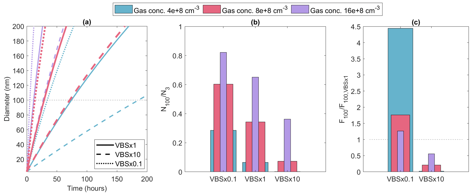
Figure 1 (a) Particle diameter as a function of time in MCOLNAG simulation with base case (solid lines) and volatilities shifted by 1 order of magnitude (dashed and dotted lines) in simulations with three different total organic vapour concentrations (indicated by line colour), (b) fraction of nucleation-mode particles reaching from initial size 3 to 100 nm in diameter, and (c) fraction of nucleation-mode particles surviving to 100 nm (F100 = N100/N3) relative to the base-case simulation.

3.2 Global aerosol–climate model ECHAM-SALSA

3.2.1 Sensitivity analysis using nine-bin VBS setup

First, we investigated how sensitive SOA burden is to the shifting of the volatility of the monoterpene oxidation products when using the nine-bin VBS setup. In Fig. 2, we present the simulated SOA burden from the base-case volatility (VBS × 1) and the relative difference in the mean SOA burden between the simulations with shifted volatilities (VBS × 10 and VBS × 0.1) and the base-case volatility (VBS × 1) for the summer period of the simulation year 2010. As expected, an increase in volatility led to a decrease in the SOA burden, while a decrease in volatility resulted in an increase in the SOA burden. A 10-fold increase in volatility led to an average reduction of 9 % in the SOA mass burden, while a 10-fold decrease in volatility resulted in a 13 % increase in the SOA mass burden over the boreal region. These changes in SOA burden are particularly noticeable over Scandinavia and throughout central Russia.

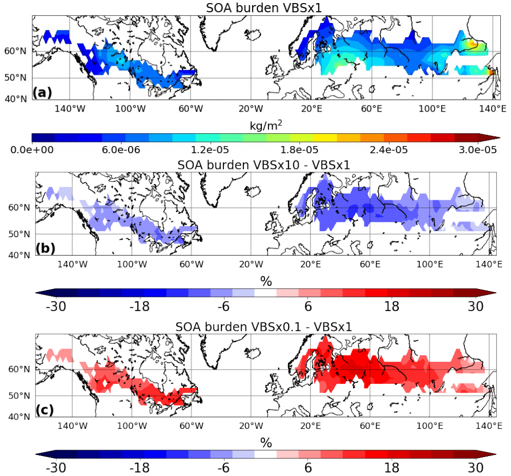
Figure 2 Simulated SOA burden of (a) VBS × 1 and the relative difference between (b) VBS × 10 and (c) VBS × 0.1 with respect to VBS × 1, focusing specifically on boreal-forest regions to emphasize the sensitivity to monoterpene SOA.

The changes in SOA mass burden with changes in volatility are consistent with the corresponding changes in the behaviour of gas–particle partitioning of the organic compounds. As the volatility of SOA decreases, the organic compounds become more likely to condense onto particles, causing more organic compounds to exist in the particle phase; on the other hand, when the volatility of SOA increases, the organic compounds are more likely to exist in the gas phase. To analyse how sensitive the SOA formation is to the shifting of volatility, we calculated the fraction of the mass partitioned in the particle phase for the three volatility assumptions (VBS × 0.1, VBS × 1 and VBS × 10) for each volatility bin (see Fig. 3). It is notable that almost all of the total mass in the lower-volatility bins with C_sat values ranging from 0 to 10⁻¹ µg m⁻³ is in the particle phase. This suggests that the SOA mass formed from these volatility bins is not sensitive to reasonable uncertainties in their volatilities. However, the biggest differences in gas–aerosol partitioning are seen in bins with C_sat values ranging from 10⁰ to 10³ µg m⁻³, i.e. bins that are not fully partitioned to either the gas or the particle phase. This means that the uncertainties associated with the volatility of these semi-volatile bins make a notable contribution to the sensitivity of the gas–particle partitioning to the shift in the volatility distribution.

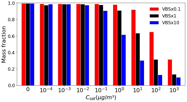
Figure 3 Fraction of particle phase-mass concentration close to the ground level (particle$/$(particle + gas)) in each VBS bin with changes in volatility depicted for the boreal-forest region. The x-axis values show the C_sat of that bin in the VBS × 1 simulation.

In order to investigate how the uncertainty in the volatility distribution affects the simulated CCN and cloud properties, we analysed how N100 and CDNC are affected when volatilities are shifted by 1 order of magnitude. Figure 4 shows the simulated burden of N100 for the VBS × 1 simulation and the relative differences between simulations with shifted volatilities (VBS × 10 and VBS × 0.1) and the VBS × 1 simulation. Similarly to the SOA burden, increasing the volatility resulted in a decrease in N100, while decreasing the volatility led to an increase in N100. The shift in volatility had a smaller impact on the CCN burden than the SOA mass burden across the study region. The relative differences ranged from −2 % to −7 % for the VBS × 10 and from 1 % to 5 % for the VBS × 0.1 compared to the VBS × 1 simulation. Similarly to the changes in SOA mass burden, increasing volatilities reduce N100, and decreasing volatilities increase N100 over almost the whole region. However, specific pressure levels exhibited a reduction in N100 with a decrease in volatility in certain parts of the study region, particularly in regions that are strongly affected by anthropogenic emissions (see Fig. S1 in the Supplement).

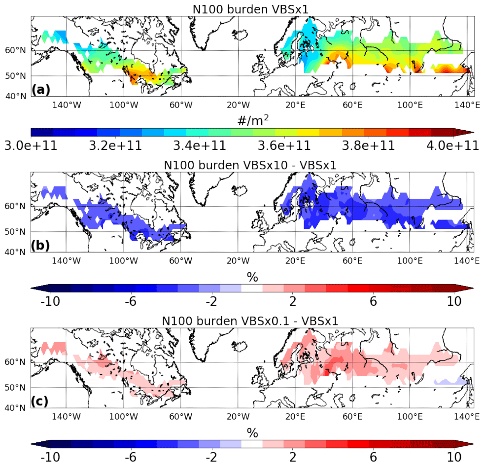
Figure 4 Simulated CCN burden of (a) VBS × 1 and the relative difference between (b) VBS × 10 and (c) VBS × 0.1 with respect to VBS × 1, focusing specifically on boreal-forest regions to emphasize the sensitivity to monoterpene SOA.

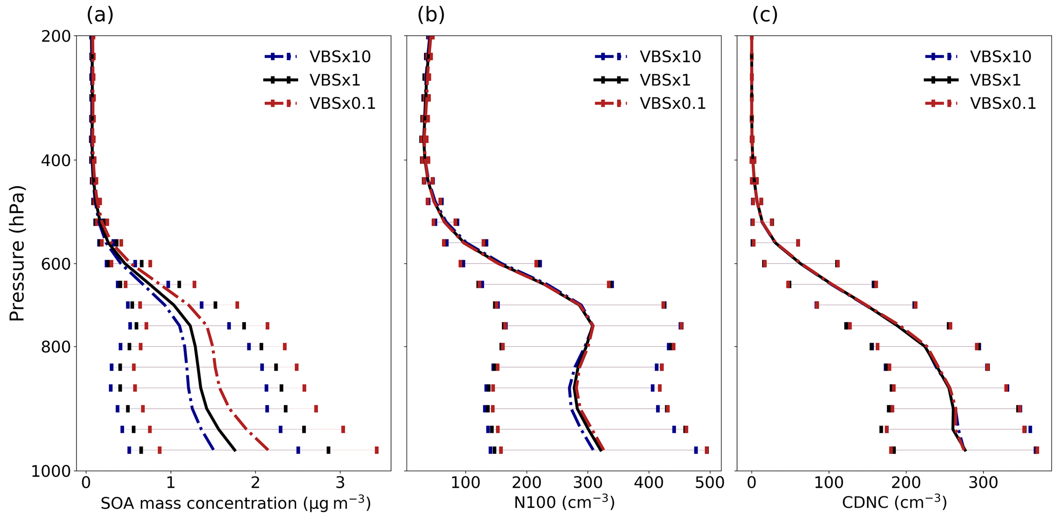
Figure 5 Mean vertical profile of (a) SOA mass concentrations, (b) N100 and (c) CDNC (grids with cloud fraction ≤ 0.95 are excluded from the calculation of CDNC) at ambient conditions for volatility-shifting simulations using nine-bin VBS setup over the boreal-forest region. The error bar depicts 1-sigma standard deviation of the data calculated across different grid cells for each model level.

Figure 5 depicts the average vertical profile of SOA mass concentrations, N100 and CDNC for the original volatility simulation (VBS × 1) and the simulations with shifted volatilities (VBS × 10 and VBS × 0.1). The mean relative difference in SOA mass concentration is found to be approximately −9 % for VBS × 10 and +13 % for VBS × 0.1 with respect to VBS × 1, as seen in Fig. 5a. Figure 5b depicts that the mean relative difference in N100 is nearly −3 % for VBS × 10 and +2 % for VBS × 0.1 with respect to VBS × 1. The changes are biggest at the heights of the typical boundary layer cloud base heights over the boreal regions, thus having an impact on cloud activation.

As shown in Fig. 5c, the changes in CDNC with changes in volatility are consistent with the behaviour of N100 with a shift in volatility. There is a very small effect of the shift in volatility on the mean CDNC analysed over the studied region. This suggests that the change in the concentration of CCN particles due to a shift in volatility does not lead to a considerable change in the concentration of cloud droplets. This could be due to the fact that changes in CDNC are influenced by a combination of factors beyond CCN concentration alone, including cloud microphysics, meteorological conditions and the aerosol composition.

The observed shifts in SOA mass concentration and particle number concentration could be attributed to the partitioning behaviour of volatile compounds within the aerosol population. Specifically, low-volatility compounds, which play a significant role in the growth of the smallest particles to CCN sizes, tend to partition to the particle phase across all VBS setups, as seen in Fig. 3. Notably, the biggest differences in partitioning occur for VBS bins with higher volatilities, which have more influence on particle masses in larger particles already having reached CCN sizes. Hence, while the overall mass changes with volatility shifts, the CCN concentration and CDNC may remain relatively unchanged.

3.2.2 Comparison between nine-bin VBS setup and three-bin VBS setup

Since increasing the number of volatility bins increases the computational cost of a global model, we also investigated how well a three-bin VBS setup compares against a more accurately resolved nine-bin VBS setup. We assessed the sensitivity of SOA burden, N100 and CDNC, comparing the otherwise identical simulations using nine-bin and three-bin VBS setups. We applied the arithmetic mean to calculate volatility in the three-bin VBS setup compared to in the nine-bin VBS setup. Based on these simulations, the nine-bin VBS setup has a higher SOA burden, up to 20 % more than the three-bin VBS setup. It should be noted that the total production of condensable organics from monoterpene oxidation between both the VBS setups remains unchanged. At the ground level, the nine-bin VBS setup has an 18 % higher SOA mass concentration than the three-bin VBS setup, as shown in Fig. 6a. The difference in mass concentration between the two VBS setups primarily comes from the variations in mass concentration within bin 3 (third bin) of the three-bin VBS setup compared to the cumulative mass concentration in the corresponding bins of the nine-bin VBS setup (see Fig. S2 in the Supplement). This results in a lower SOA mass concentration being observed in the three-bin VBS setup. However, it is worth noting that the mass concentrations in the other two low-volatility bins in the three-bin VBS setup remain consistent with the cumulative mass concentrations in their corresponding bins from the nine-bin VBS setup. These differences between the two setups highlight the sensitivity of their configurations to the selection of volatilities assigned to each bin in the three-bin VBS setup.

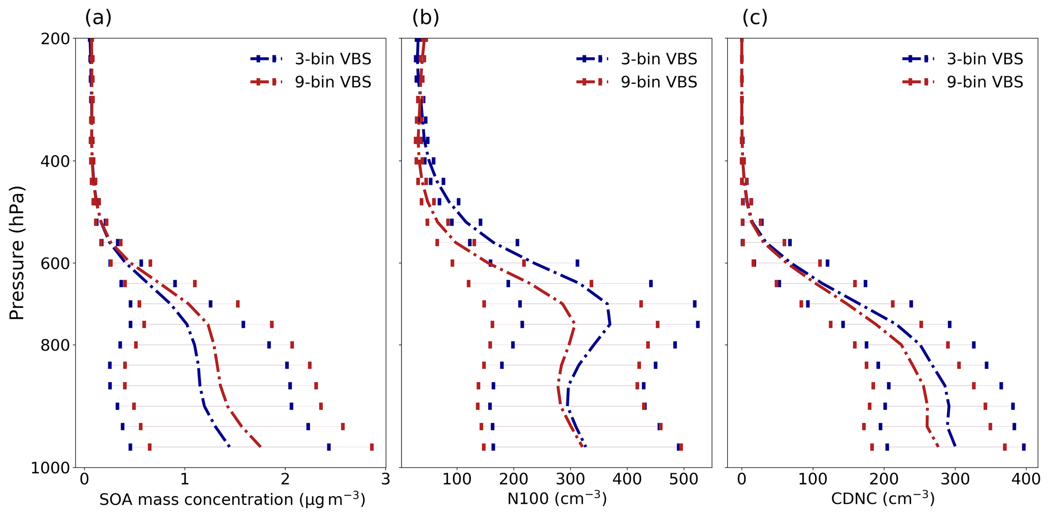
Figure 6 Mean vertical profile of (a) SOA mass concentrations, (b) N100 and (c) CDNC (grids with cloud fraction ≤ 0.95 are excluded for the calculation of CDNC) at ambient conditions for the VBS × 1 simulation using nine-bin and three-bin VBS setups over the boreal-forest region. The error bar depicts 1-sigma standard deviation of the data calculated across different grid cells over each model level.

There is also a notable difference in the N100 concentration between the nine-bin VBS setup and three-bin VBS setup, as illustrated in Fig. 6b. The difference in N100 between the nine-bin VBS setup and the three-bin VBS setup is in the opposite direction as compared to the SOA mass; i.e. the three-bin VBS setup has a higher N100 concentration than the nine-bin VBS setup. Specifically, at around 500 hPa, the three-bin VBS setup has approximately 70 % higher N100 compared to the nine-bin VBS setup. However, the difference in N100 between the two setups is only approximately 5 % close to the ground level. In other words, the VBS with a lower number of volatility bins can result in higher N100 compared to the VBS with a higher number of volatility bins, although the SOA mass shows the opposite behaviour. This could be because a lower number of volatility bins in the VBS leads to a broader volatility range being assigned to each bin, which can lead to a higher concentration of SOA particles. Figure 6c demonstrates that there is an increase in CDNC in the three-bin VBS setup when compared with the nine-bin VBS setup. This is in line with the higher N100 observed in the three-bin VBS setup. The higher N100 in the three-bin VBS setup resulted in an increase of approximately 10 % in CDNC compared to the nine-bin VBS setup. It is worth noting that we also explored the geometric mean to calculate the volatility of the three-bin VBS setup based on the nine-bin VBS setup, which resulted in better SOA mass matching between the two setups but worse matching for N100 (see Fig. S3 in the Supplement).

3.2.3 Sensitivity of N100 to the volatility of individual VBS bins

To better understand the sensitivity of SOA mass and CCN concentration to uncertainties in the volatilities of individual VBS bins, a series of simulations were conducted in which the volatility of one VBS bin was shifted by 1 order of magnitude at a time, while the volatilities of other bins were kept unchanged. These simulations were performed in the global aerosol–climate model ECHAM-SALSA using the three-bin VBS setup. Each bin in the three-bin VBS setup is represented as bin 1, bin 2 and bin 3 by order of increasing volatility.

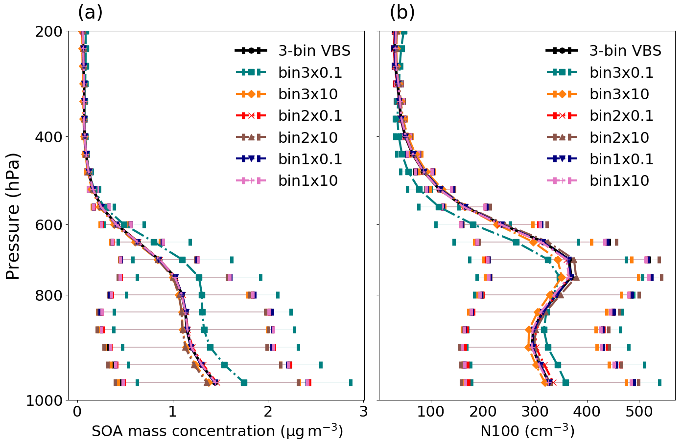
Figure 7 Mean vertical profile of (a) SOA mass concentrations and (b) N100 at ambient conditions when the VBS bins are shifted individually using the three-bin VBS setup over the boreal-forest region. The error bar depicts 1-sigma standard deviation of the data calculated across different grid cells over each model level.

Figure 7 depicts the effect of a 1-order-of-magnitude shift in volatility of individual VBS bins on the SOA mass concentration and N100 over the studied region. The volatilities in the three bins, bin1, bin2 and bin3, are 4.8 × 10⁻⁴, 5.48 × 10⁻¹ and 5.32 × 10²  µg m⁻³, respectively, as described in Sect. 2.3. The change in bin 1 (the lowest-volatility class) does not seem to have any effect on either SOA mass concentration or N100. However, the increase in the volatility of bin 2 led to a decrease of approximately 7 % in SOA mass and a 3 % decrease in N100, and a decrease in volatility lead to a nearly 4 % increase in SOA mass and a 3 % increase in N100. Bin 3 (the highest-volatility class) is found to be the most sensitive VBS class in relation to the changes in volatility. An increase of 1 order of magnitude in the volatility of bin 3 led to a mean decrease of around 5 % in SOA mass and 2 % in N100, while a decrease in the volatility of bin 3 led to an increase of approximately 20 % in SOA mass and a 9 % increase in N100. When shifting the entire three-bin VBS distribution, a 10-fold increase in volatility led to a notable 24 % increase in SOA mass, and a 10-fold decrease in volatility resulted in an 8 % reduction in SOA mass concentration. As bin 3 corresponds to the semi-volatile class in the VBS distribution, a significant amount of organic matter in this bin resides in both the gas phase and the particle phase. Bin 3 bundles the nine-bin setup bins with C_sat values of 10⁻², 10⁻¹ and 10⁰ µg m⁻³ (see Fig. 3). Out of these three bins, only the highest-volatility bin is sensitive to the shift in volatility, whereas combining them into one bin in the three-bin VBS setup makes the 10⁻²–10⁰ µg m⁻³ volatility range sensitive to the assumed mean volatility of the bin (see Fig. S4 in the Supplement). This is also the reason why shifting one bin in the three-bin VBS setup affects the change in N100 and SOA mass, as shown in Fig. 7, rather than shifting the whole nine-bin distribution, as shown in Fig. 5. Overall, this test emphasizes the need to carefully select the volatilities of VBS bins when fewer bins are used in models so that the model reproduces a more highly resolved VBS bin setup.

3.2.4 Effect of volatility distribution on radiative forcing

As discussed, SOA influences radiative forcing through both direct and indirect effects. According to O'Donnell et al. (2011), the estimated global mean SOA direct effect is −0.31 W m⁻², while the indirect effect is +0.23 W m⁻². However, it is important to note that a substantial uncertainty exists among different models, with a range of up to 1 W m⁻² in the radiative effects of SOA, particularly for the first aerosol indirect effects (Zhu et al., 2017). Here, we assessed how the sensitivities in simulated aerosol and cloud properties to the assumptions regarding the volatility distribution affect the radiative properties of the simulated atmosphere. Specifically, we explored the radiative forcing due to aerosol–radiation and aerosol–cloud interactions. This section presents the quantified shortwave IRF_ari and shortwave ERF for different volatility-shifting simulations employing different numbers of volatility bins. Figure 8 shows the IRF_ari and ERF for a 1-order-of-magnitude volatility shift with respect to the original volatility using the nine-bin VBS setup and between the three- and nine-bin VBS setups from the VBS × 1 simulation. The decrease in SOA burden due to the 1-order-of-magnitude increase in volatility contributes to a positive radiative forcing (RF) with respect to the original volatility in the nine-bin VBS setup. Similarly, an increase in SOA burden due to a corresponding decrease in volatility leads to a more negative RF compared to that of the original volatility distribution. The IRF_ari is found to be +0.16 ± 0.07 and −0.2 ± 0.08 W m⁻² for the VBS × 10 and VBS × 0.1 simulations, respectively, with respect to the VBS × 1 simulation, while ERF is +0.35 ± 2.1 and −0.4 ± 2.3 W m⁻² for the VBS × 10 and VBS × 0.1 simulations, respectively, relative to the VBS × 1 simulation. Additionally, we estimated IRF_ari and ERF from a scenario with the SOA being shut off relative to the VBS × 1 simulation. The IRF_ari of SOA over the boreal-forest region is −0.18 W m⁻², and the ERF is −1.03 W m⁻², highlighting the significant cooling effect of SOA in this region.

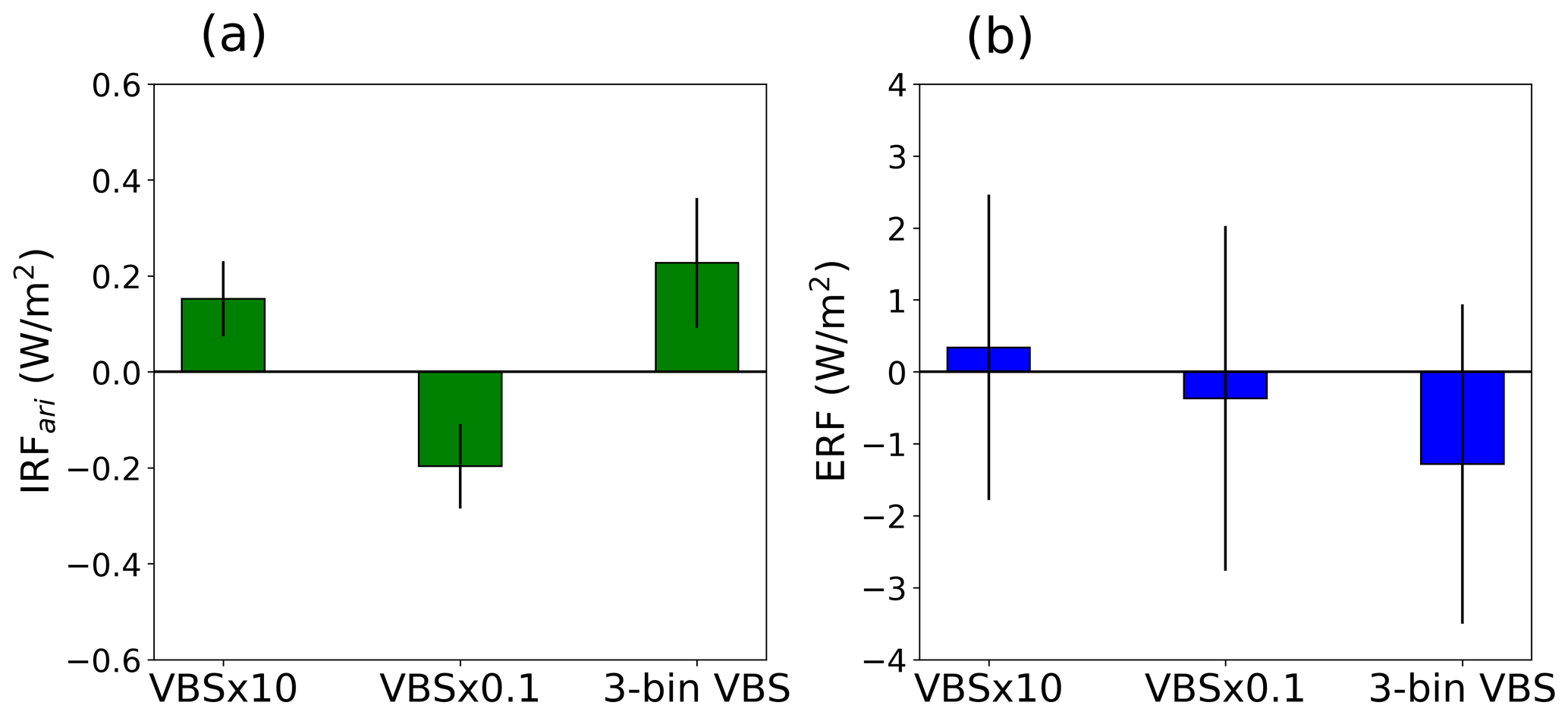
Figure 8 Summer mean (a) TOA IRF_ari and (b) ERF for the shift in volatility by 1 order of magnitude with respect to the base volatility using the nine-bin VBS setup and the base volatility in the three-bin VBS setup relative to that in the nine-bin VBS setup, estimated over the boreal-forest region. Error bar depicts 1-sigma standard deviation of the data calculated across different grid cells.

On the other hand, the base volatility in the three-bin VBS setup results in a positive IRF_ari and a negative ERF with respect to the base volatility in the nine-bin VBS setup. This is because the three-bin VBS setup has a lower SOA mass and a higher particle number concentration as compared to the nine-bin VBS setup. The summer mean IRF_ari and ERF for the three-bin VBS setup are found to be +0.25 ± 0.1 and −1.25 ± 2.2 W m⁻², respectively, relative to the base volatility in the nine-bin VBS setup. The positive IRF_ari and negative ERF in the three-bin VBS setup are more pronounced over Russia while being the least pronounced over the northern US, as shown in Fig. S5 in the Supplement.

The results in Fig. 9 show the IRF_ari and ERF calculated for simulations using a three-bin VBS setup, where the volatilities of individual volatility bins are shifted relative to the base volatility. The findings indicate that the changes in radiative forcings are consistent with the difference in SOA mass and N100 due to the shift in the volatility of individual VBS bins. The results reveal that the distribution of organic aerosol volatility substantially influences radiative forcing, encompassing both the IRF_ari and ERF components of radiative fluxes. Similarly to SOA mass and N100, the shift in the volatility of the highest-volatility bin (bin 3) causes the largest effect in radiative forcing. The decrease in the volatility of bin 3 by 1 order of magnitude (bin 3 × 0.1) leads to a cooling effect of −0.2 ± 0.1 W m⁻² in IRF_ari and a warming effect of 0.8 ± 2.24 W m⁻² in ERF relative to the base volatility in the three-bin VBS setup. The negative IRF_ari and positive ERF from bin 3 × 0.1 are attributed to the lower number concentrations and the higher SOA mass as compared to the base volatility using the three-bin VBS setup. Conversely, increasing the volatility of bin 3 by 1 order of magnitude (bin 3 × 10) induces a warming effect for both IRF_ari and ERF. The corresponding values for the increased volatility scenario are 0.05 ± 0.04 W m⁻² for IRF_ari and 0.45 ± 2.3 W m⁻² for ERF. Conversely, the shifts in the volatilities of bin 2 and bin 1 have minor effects on the radiative forcing.

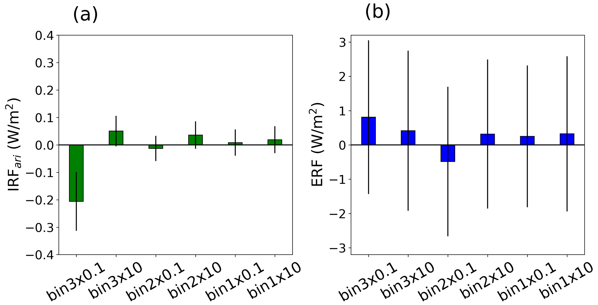
Figure 9 Summer mean (a) TOA IRF_ari (b) ERF for the shift in volatility of individual volatility bins with respect to the base volatility using the three-bin VBS setup estimated over the boreal-forest region. Error bar depicts 1-sigma standard deviation of the data calculated across different grid cells.

4 Conclusions

This study demonstrates the importance of an accurate representation of semi-volatile organics in a global-scale model to simulate aerosol–climate interactions. The volatility distribution of organics is crucial, especially because it determines the partitioning of these compounds between the gas and particle phases. The partitioning process is essential for accurately simulating aerosol formation and growth processes in the atmosphere (Williams et al., 2010). In this study, we conducted a series of simulations using the process-scale model MCOLNAG and the global aerosol–climate model ECHAM-SALSA to examine, in particular, how sensitive the CCN is to the volatility assumptions of organic compounds. Although the process model simulations show a high sensitivity of CCN to the uncertainties associated with the volatilities of condensing organic vapours, the global-model simulations with the highly resolved nine-bin VBS setup show that N100 and CDNC are insensitive to a 1-order-of-magnitude shift in volatility. However, a notable difference was observed in the global-model-simulated SOA mass burden. It was also found that nearly all of the total mass in the lower-volatility bins of the nine-bin VBS setup, with C_sat values up to 10⁻¹, remained in the particle phase, while the bins with C_sat values from 10⁰ contributed to the sensitivity of gas–particle partitioning. This behaviour of gas–particle partitioning indicates that the lower-volatility bins are insensitive to reasonable uncertainties in their volatilities, whereas the higher volatilities with C_sat values of 10⁻¹ µg m⁻³ or higher are highly sensitive to their volatilities. This suggests that the semi-volatile bins in the VBS setups require higher resolutions than the low-volatility compounds in a global model. Essentially, if a global model needs to represent organic compounds in fewer volatility bins then, ideally, the lower-volatility bins with C_sat values up to 10⁻¹ can be lumped together into a single bin, while the remaining bins can have finer representations. Additionally, the global-model analysis indicated that the SOA mass burden, N100 and radiative forcing were most sensitive to the uncertainties associated with the volatility of semi-volatile bins rather than the low-volatility bins. The simulations also show that the IRF_ari is sensitive to uncertainties in volatility in the nine-bin VBS setup, while the ERF becomes sensitive only if the simplified three-bin VBS setup is used, as is made evident by the larger uncertainty associated with ERF changes. For example, in the VBS × 10 scenario, the IRF_ari is +0.16 ± 0.07 W m⁻², while the corresponding ERF is +0.35 ± 2.1 W m⁻². This highlights the importance of accurately representing the volatility of such compounds in global-scale models to improve the accuracy of capturing aerosol properties and their impacts on the climate. Furthermore, our comparison between the highly resolved VBS setup with nine volatility bins and a simpler VBS setup with three volatility bins revealed a remarkable difference in N100 and CDNC. The three-bin VBS setup exhibited higher N100 and CDNC compared to the nine-bin VBS setup but lower SOA mass concentrations. These findings highlight the need for careful assessment when reducing the number of volatility bins and selecting appropriate values for volatility. We applied the arithmetic mean to calculate volatility in the three-bin VBS setup based on the nine-bin VBS setup. While using the geometric mean for calculating the volatility resulted in improved agreement in terms of SOA mass between the two setups, it led to less accurate matching for N100. Hence, choosing a value for volatility is a balance between getting the correct particle number concentration or SOA mass concentration.

For future studies, it would be valuable to investigate the optimal VBS setup for a small number of volatility bins, aiming to strike a balance between computational efficiency and scientific accuracy. Such research could provide insights into achieving optimal speed and accuracy in modelling efforts related to aerosol properties and their implications for the climate. Moving forward, our study also underscores the necessity of incorporating data from volatility experiments involving diverse compositions into global-modelling studies. Currently, volatility observations mostly focus on single compositions, limiting their ability to capture atmospherically relevant conditions. Components like brown carbon, dust aerosols and sea sprays are prevalent in the atmosphere, and their inclusion in volatility-based studies is required. Integrating such data is crucial for constraining the parameterizations of VBS bins in global models, thereby ensuring a comprehensive representation of aerosols.