the Creative Commons Attribution 4.0 License.
the Creative Commons Attribution 4.0 License.
 | 24 Jul 2024
A systematic evaluation of high-cloud controlling factors
Sarah Wilson Kemsley
Paulo Ceppi
Hendrik Andersen
Jan Cermak
Philip Stier
Peer Nowack
Clouds strongly modulate the top-of-the-atmosphere energy budget and are a major source of uncertainty in climate projections. “Cloud controlling factor” (CCF) analysis derives relationships between large-scale meteorological drivers and cloud radiative anomalies, which can be used to constrain cloud feedback. However, the choice of meteorological CCFs is crucial for a meaningful constraint. While there is rich literature investigating ideal CCF setups for low-level clouds, there is a lack of analogous research explicitly targeting high clouds. Here, we use ridge regression to systematically evaluate the addition of five candidate CCFs to previously established core CCFs within large spatial domains to predict longwave high-cloud radiative anomalies: upper-tropospheric static stability (SUT), sub-cloud moist static energy, convective available potential energy, convective inhibition, and upper-tropospheric wind shear (ΔU300). We identify an optimal configuration for predicting high-cloud radiative anomalies that includes SUT and ΔU300 and show that spatial domain size is more important than the selection of CCFs for predictive skill. We also find an important discrepancy between the optimal domain sizes required for predicting locally and globally aggregated radiative anomalies. Finally, we scientifically interpret the ridge regression coefficients, where we show that SUT captures physical drivers of known high-cloud feedbacks and deduce that the inclusion of SUT into observational constraint frameworks may reduce uncertainty associated with changes in anvil cloud amount as a function of climate change. Therefore, we highlight SUT as an important CCF for high clouds and longwave cloud feedback.
- Article
(10277 KB) - Full-text XML
-
Supplement
(3801 KB) - BibTeX
- EndNote


Changes in clouds are the primary source of uncertainty in the quantification of equilibrium climate sensitivity (ECS) – the long-term global warming response to a doubling of atmospheric carbon dioxide (Sherwood et al., 2020; Zelinka et al., 2022). Cloud-induced radiative anomalies (R) at the top of the atmosphere (TOA) refer to changes in the balance of incoming and outgoing radiation caused by interaction with clouds. While most evidence suggests that the change in R at the TOA as a function of global warming likely has a positive effect on Earth's energy balance and thus amplifies warming (e.g., Ceppi and Nowack, 2021), the magnitude of this global cloud feedback remains highly uncertain (Ceppi et al., 2017; Sherwood et al., 2020; Zelinka et al., 2022).
Motivated by the role of clouds as a key uncertainty factor, much progress has been made towards understanding the mechanisms that drive changes in R, considering different cloud types under both natural unforced variability and long-term climate change. In particular, such work includes theoretical understanding of cloud feedback processes (e.g., Zelinka and Hartmann, 2010; Rieck et al., 2012; Bony et al., 2016), idealized regional modeling studies (Bretherton, 2015; Siebesma et al., 2003), convection-permitting global climate models (Hentgen et al., 2019), and climate model evaluation studies (Zelinka et al., 2022).
Here, we aim to systematically advance an alternative approach widely used for understanding and constraining uncertainties in cloud variability and trends in the form of cloud controlling factor (CCF) analysis. Exploiting observed relationships between large-scale satellite cloud observations and meteorological predictor variables, CCF analyses have, for example, been used to derive observational constraints on cloud-related uncertainty estimates (Myers and Norris, 2016; Andersen et al., 2017, 2022; Fuchs et al., 2018; Ceppi and Nowack, 2021; Myers et al., 2021). In particular, meteorological CCFs for low marine and boundary layer clouds have been widely assessed (Andersen et al., 2022; Brient and Schneider, 2016; Klein et al., 2017; Qu et al., 2015; Scott et al., 2020), with typical frameworks including CCFs such as surface temperature (Tsfc), temperature advection, estimated boundary layer inversion strength (EIS), vertical velocity, 700 hPa relative humidity (RH700), and near-surface wind speed. However, comparatively less research has specifically targeted the CCFs for high clouds despite their significant – and highly uncertain – contributions towards the total estimated feedback (Sherwood et al., 2020). A systematic comparison of CCF candidates for high clouds within a range of spatial domains will therefore be the main subject of this paper.
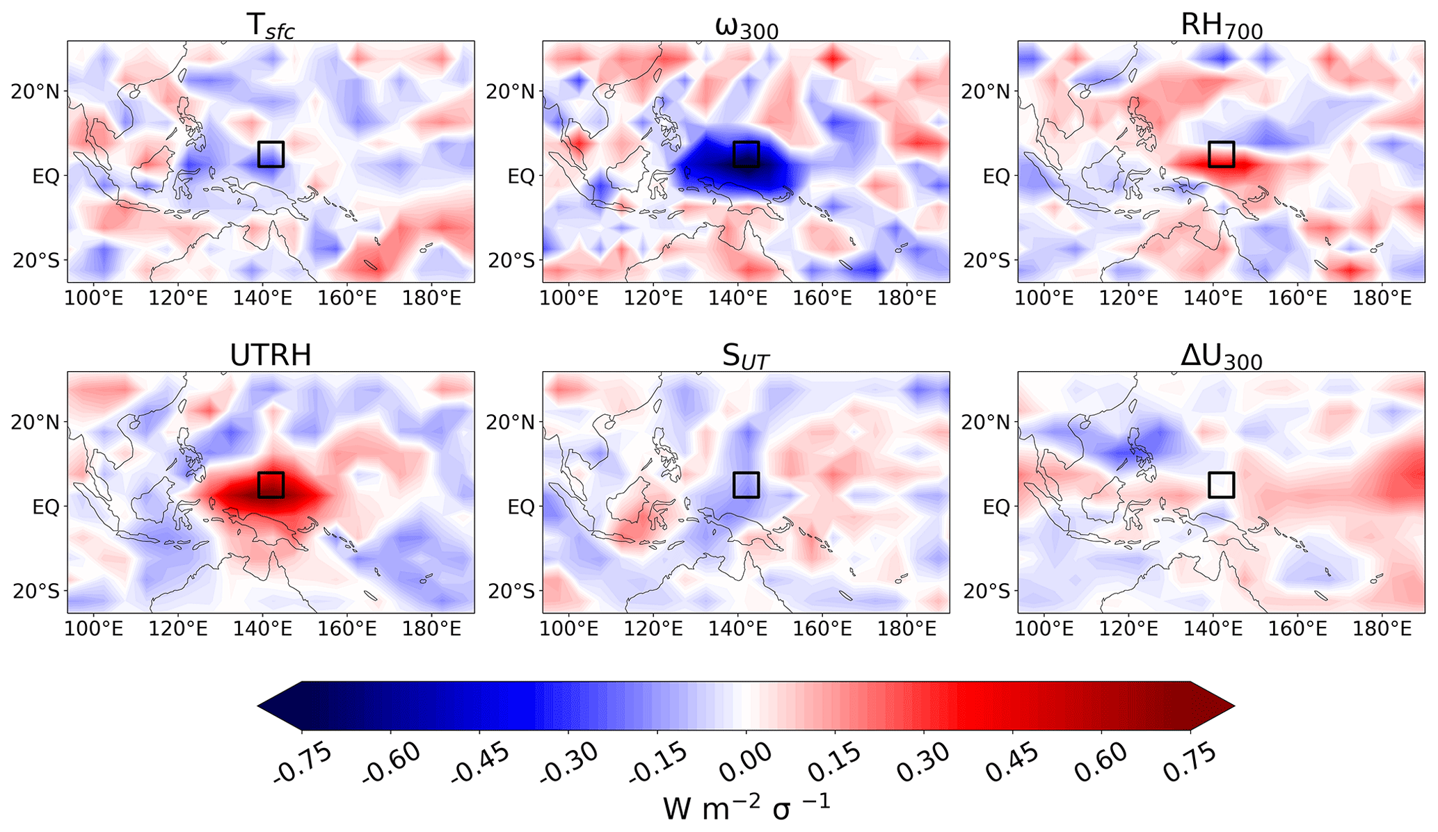
Figure 1CMIP multi-model mean longwave cloud radiative sensitivities for a sample 5°×5° target grid box (center 2.5° N, 142.5° E indicated by the black box) to surface temperature (Tsfc), vertical velocity at 300 hPa (ω300), relative humidity at 700 hPa and in the upper troposphere (RH700 and UTRH, respectively), wind shear at 300 hPa (ΔU300), and upper-tropospheric static stability (SUT) using a 21×11 domain of grid boxes around the target (corresponding to 110° longitude × 55° latitude area, centered on the grid box). Radiative anomalies are normalized for a 1-standard-deviation (σ) anomaly in the controlling factors based on monthly variability.
Our work builds on a modification to a previous CCF approach, which was introduced by Ceppi and Nowack (2021, hereafter CN21). CN21 used ridge regression for their analyses, which allowed them to consider large spatial domains of CCF predictor patterns around target grid points in which cloud radiative anomalies were predicted, with an example shown in Fig. 1. This approach contrasts with previous CCF analyses using standard multiple linear regression, which are constrained to a small number of predictors (typically < 10). This allowed their analysis to be extended beyond specific cloud regimes. As shown in CN21, the consideration of larger-scale CCF patterns led to improvements in predictive skill for both shortwave (SW) and longwave (LW) global cloud feedback. The intuition behind using spatial patterns of CCFs is motivated by the synoptic-scale atmospheric system within which the life cycle of clouds – from formation to cessation – occurs, resulting in more robust predictions of global cloud feedback. Non-local features, such as large-scale patterns of sea surface temperature anomalies and changes in the atmospheric circulation (e.g., convergence and divergence), are implicitly encoded using large spatial domains, which are not included in scalar CCF analysis despite their relevance for the context in which cloud development occurs (when considering monthly averaged data typically used for CCF analyses; Klein et al., 2017). Altogether, considering larger-scale patterns resulted in better out-of-sample predictions, which consequentially tightened the cloud-induced uncertainty in general circulation model (GCM)-modeled ECS.
However, the framework introduced by CN21 highlighted an important limitation. As the same set of five CCFs were used for SW and LW analyses, their predictive skill was markedly stronger for global SW and net feedback components than for LW. Given that LW feedback is largely driven by high clouds while SW feedback is instead predominantly driven by the oft-studied low clouds, we speculate the performance deficit may be – at least to a degree – a symptom of CCF choice. Indeed, Zelinka et al. (2022) specifically recommend that the drivers of high-cloud feedback must be targeted to reduce cloud-related uncertainty in ECS estimates.
To address these open questions, we use ridge regression to methodically assess candidate CCFs of high clouds within a range of spatial scales, aiming to inform CCF choice for future observational constraints on the ECS uncertainty. Here, we target LW cloud radiative anomalies (RLW) as they are more directly associated with high clouds than SW (and consequently net) radiative anomalies. We briefly assess implications of CCF choices for net anomalies, RNET, noting that, historically, LW and SW high-cloud radiative anomalies tend to offset each other, resulting in little net signal for thick clouds over monthly timescales. We therefore restrict our analysis to clouds with top pressures smaller than 680 hPa; future references to “R” are therefore specifically emanating from these non-low clouds (see Sect. 3.1 for the dataset used). Though radiative effects from midlevel clouds are also by definition included in our analysis, we collectively refer to radiative anomalies as “high” henceforth for simplicity (Zelinka et al., 2016).
We systematically assess static stability in the upper troposphere (SUT), sub-cloud moist static energy (m), convective available potential energy (CAPE), convective inhibition (CIN), and upper-tropospheric wind shear (ΔU for easterly shear) as CCFs based on their physical relationships with high-cloud properties or convection, with an overview presented in Sect. 2. Aiming to inform choices for future observational constraint analyses, we only suggest CCFs that are readily available (or easily calculated from measurable quantities). Alternative variables, such as the radiatively driven divergence, horizontal mass convergence, and gross moist stability, may also capture high-cloud properties, but their derivation requires numerical modeling, and hence we do not consider them here. Sections 3 and 4 discuss the data and methods we use, respectively, with combined results and discussion presented in Sect. 5. We first discern which CCF combinations can best predict out-of-sample grid-cell-scale historical internal variability. We then investigate which combinations best predict out-of-sample globally aggregated RLW. Based on the results of our statistical testing, we physically interpret the coefficients for a single (optimal) configuration of CCFs and assess whether the spatial pattern, magnitude, and variability of the cloud properties (i.e., cloud-top pressure and cloud fraction) are accurately captured.
Ubiquitously present over the tropics, cirrus, cirrostratus, and deep convective clouds are responsible for the largest annual mean changes in global TOA LW flux (Chen et al., 2000). Tropical cirrus clouds develop through one of two mechanisms: in situ ice formation that is not associated with convection or outflow from deep convective cores (Gasparini et al., 2023; Kärcher, 2017). Large-scale ascent in the tropical tropopause layer results in adiabatic cooling and high relative humidity, creating an ideal environment for in situ ice formation, typically at heights above the level of deep convective outflow (Fueglistaler et al., 2009; Gasparini et al., 2023). Convective outflow cirrus (referred to as “anvil cirrus”), together with a mature cumulonimbus core, forms tropical anvil clouds. “Thick” cirrus clouds are both effective absorbers of upwelling LW radiation and also efficient reflectors of incident SW radiation. Over time, dynamical, radiative, and microphysical processes can spread the thick anvil cirrus, extending anvil lifetime and resulting in larger cloud cover than the initial convective core (Gasparini et al., 2019, 2023; Luo and Rossow, 2004). Such processes can result in the formation of “thin” cirrus clouds, characterized by a relatively smaller SW cloud radiative forcing compared to LW (Fueglistaler et al., 2009; Jensen et al., 1994; McFarquhar et al., 2000). Though deep convective clouds presently have relatively small abundance (compared to other cloud types), their local radiative effects are large (Chen et al., 2000), and therefore changes to their frequency of occurrence can have substantial impacts on cloud feedback. Despite this, most previous CCF analyses focused on low-cloud regimes so that the selection and design of CCFs were mainly motivated by meteorological situations driving cloud formation and cessation in those cloud regimes (Klein et al., 2017).
In CN21, a compromise was sought by considering classic CCFs such as Tsfc, EIS, and RH700 (relative humidity at 700 hPa) but by also using the vertical velocity at 500 hPa (ω500) and upper-tropospheric relative humidity (UTRH, the vertically averaged relative humidity in the 200 hPa layer below the tropopause) as predictors in an attempt to additionally target high clouds. In the following, we will build on the CN21 CCF setup, specifically targeting modifications and additions that are more likely to represent state variables important for the aforementioned high clouds. One by one we will examine these CCF candidates physically and formally define them, before testing the prediction results of possible CCF combinations for high clouds in Sect. 5.
An overview of all CCFs considered and their scientific motivations is summarized in Table 1. We keep Tsfc, RH700, UTRH, and ω (at variable pressure levels) in all configurations, which we refer to as the “core” CCFs, as they jointly explain a large portion of historical variability in RLW and are each physically related to high-cloud formation. The large-scale distribution of tropical deep clouds is closely tied to the distribution of sea surface temperatures (SSTs) and upper-tropospheric relative humidity (Bony et al., 1997; Li et al., 2014), with research indicating that lower free-tropospheric relative humidity regulates the mean height of convective outflow (Sherwood et al., 2004). Vertical velocities (ω) indicate regions of subsidence or ascent, with enhanced ascending motion supporting thicker, higher cloud layers (Ge et al., 2021). Andersen et al. (2023) find that the magnitude of (local) sensitivity to ω is largest at 300 hPa; hence we test vertical velocity at both 300 and 500 hPa (used in CN21) in this study.
Table 1High-cloud controlling factors used in CN21 and proposed here, physical explanations connecting them to high clouds or convection, and the key studies supporting them. References to “clouds” in this table are for high clouds only. EIS is not a core CCF, and therefore for conciseness we include EIS under the “Candidate CCFs” subheading.
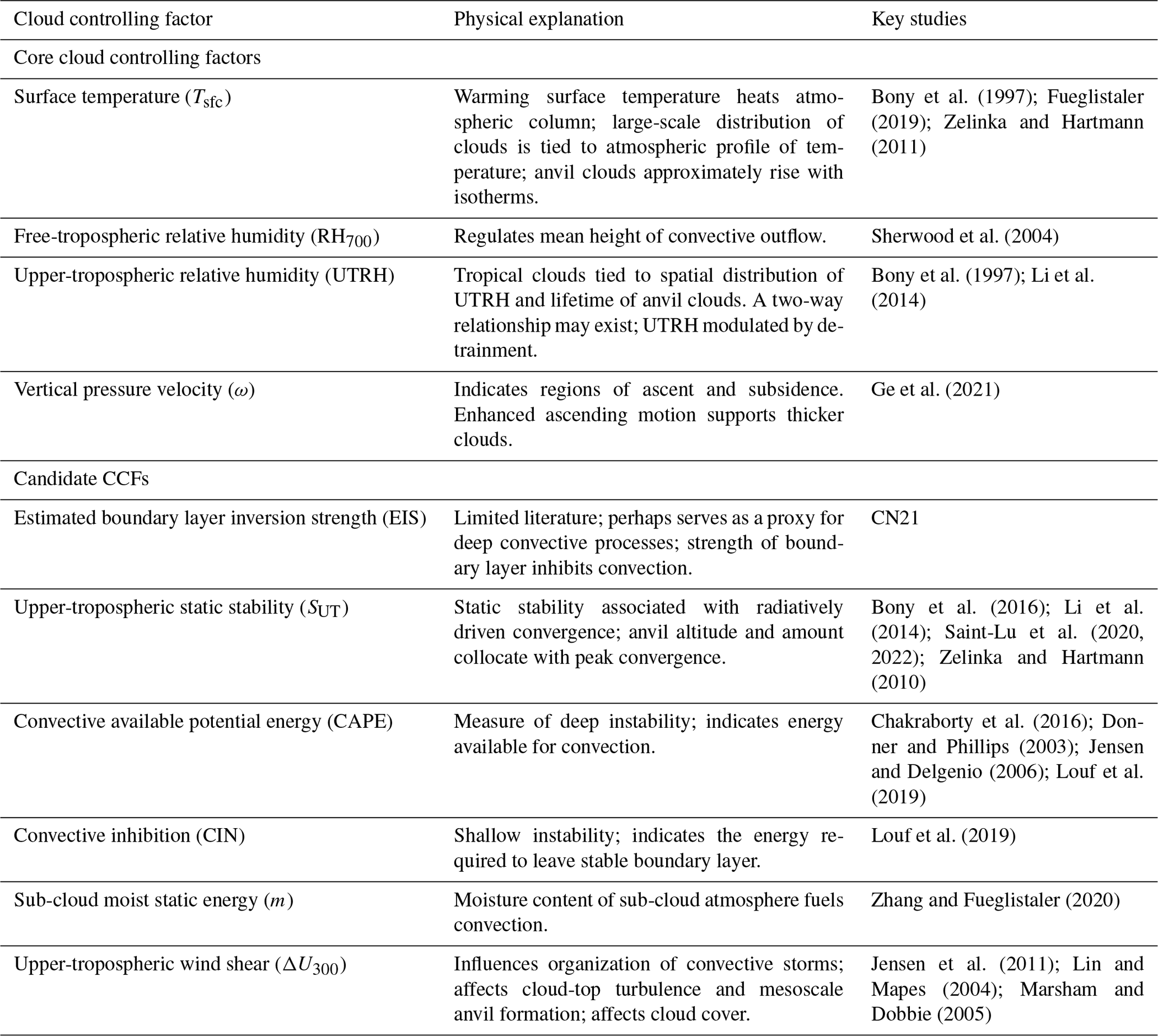
Estimated boundary layer inversion strength (EIS) is not typically regarded as a controlling factor for high clouds specifically despite its wide use in general and low-cloud CCF analyses. This results in relatively little literature interpreting high-cloud sensitivities to EIS. Despite this, CN21 used only the Tsfc and EIS sensitivities to observationally constrain global cloud feedback for both SW and LW components. These sensitivities are suitably decoupled from the clouds and still achieve good (albeit poorer than SW and net) predictions for global LW feedback. We therefore suggest five candidate CCFs as replacements for EIS that more directly represent convective processes or high-cloud formation and that are also sufficiently external to the clouds themselves and may be similarly used in constraints.
We list candidate CCFs (and EIS) and discuss them in turn below, with the exact definitions provided in Sect. 3.2:
-
Static stability is the vertical gradient of potential temperature, measuring the stratification of the atmosphere (Grise et al., 2010). Upper-tropospheric static stability is robustly (negatively) correlated with upper-level cloud incidence over much of the global ocean (Li et al., 2014) and has been observationally linked with changes in tropical anvil cloud fraction through the “anvil iris” thermodynamic mechanism (Bony et al., 2016; Saint-Lu et al., 2020, 2022). We expect increases in local upper-tropospheric static stability to result in local reductions in high-cloud fraction, with suppressed vertical motion.
-
Moist static energy characterizes the energy of an air parcel in a moist environment, considering its internal energy (latent and sensible heat) and potential energy due to its elevation. Sub-cloud moist static energy (m) may affect cloud formation, as higher levels of m signify increased potential for uplift and condensation. Additionally, when buoyant air from the boundary layer fills the free troposphere, it can inhibit the initiation of convection in colder regions, setting a threshold that hinders further upward movement (Srinivasan and Smith, 1996; Zhang and Fueglistaler, 2020). We suggest that high m increases local high cloudiness, while in contrast, we hypothesize that non-local m can either decrease (due to convective thresholds) or increase cloudiness (depending on horizontal transport).
-
Convective available potential energy (CAPE) is a measure of deep instability, describing the amount of energy available for an air parcel to rise freely through the atmosphere. CAPE offers insights into the onset, genesis, and scale of atmospheric deep convection and has been described as the fuel for a thunderstorm (Donner and Phillips, 2003; Jensen and Delgenio, 2006; Riemann-Campe et al., 2009). We speculate increased CAPE suggests an environment conducive to sustaining deep convection and thus more high cloud.
-
Convective inhibition (CIN), a form of conditional instability and CAPE's opposing parameter, is a measure of the amount of energy required for a parcel to overcome a stable layer of air and initiate the development of deep convection. A large absolute value of CIN may indicate a stable atmosphere and thus unfavorable conditions for the development of deep convective clouds (Louf et al., 2019). Note that high CIN is a required precursor for the buildup of CAPE. Once CIN has been overcome, conditions are favorable for deep convection.
-
Wind shear, defined here as the vertical change in horizontal wind speed, is an important dynamical characteristic of the upper troposphere. Wind shear influences the organization of convective storms and mesoscale convective systems in various ways, though understanding its relationship with cloud properties has proven historically challenging (Anber et al., 2014). However, studies suggest that wind shear can increase cloud-top turbulence, spread and stretch clouds horizontally through the advection of air at different levels and speeds, and hasten cirrus cloud dissipation (Jensen et al., 2011; Lin and Mapes, 2004; Marsham and Dobbie, 2005). We speculate wind shear mainly affects high-cloud fraction.
-
Estimated inversion strength (EIS) describes the strength of the boundary layer, is a dominant control for low clouds (Andersen et al., 2022, 2023; Wood and Bretherton, 2006), and is widely used in general CCF analysis (CN21; Klein et al., 2017). However, EIS is not considered a driver of high-cloud incidence, but CN21 suggested that EIS may function as a proxy for factors relating to deep convection.
Note that several candidate CCFs are not independent. For example, high values of CIN are required for a buildup of CAPE, and a stable boundary layer may be represented by both high CIN and high EIS.
We use monthly-mean (unless explicitly mentioned otherwise) cloud property and CCF data, re-gridded to a common 5° × 5° resolution. At these spatial and temporal scales, we expect the clouds to be approximately in equilibrium with their environment (Klein et al., 2017). To represent observed cloud radiative data, we use combined Moderate Resolution Imaging Spectroradiometer (MODIS) retrievals from both Aqua and Terra instruments, identified as MCD06COSP (Pincus et al., 2023). These retrievals are included as part of the CFMIP Observation Simulator Package (COSP, where CFMIP refers to the Cloud Feedback Model Intercomparison Project), which facilitates the evaluation of models against observations in a consistent manner (Bodas-Salcedo et al., 2011). For climate model data, we use 18 GCMs that have run the International Satellite Cloud Climatology Project (ISCCP) simulator (Zelinka et al., 2012a) from the Coupled Model Intercomparison Project phases 5 and 6 (CMIP5/6). For a full list of CMIP models used in this research, see Supplement Sect. S1. For the meteorological CCFs we use ERA5 reanalysis data at monthly resolution, except for CAPE and CIN, which we first calculate using daily air temperature and relative humidity profiles and then take the monthly mean. We use reanalysis data as a proxy for direct observations; henceforth, when “observed” results are discussed, we refer to predictions made for observed radiative anomalies using ERA5 meteorological CCFs.
We restrict the CMIP datasets to 20 years, aligned with the length of the available observational record, though with slightly different time periods. For observations, data are available from July 2002 to June 2022. For the CMIP models, we use historical data from January 1981 to December 2000. We use this period because it is close to the present-day climate, under the constraint of availability of historical CMIP data (and noting that only a small set of models provide satellite simulator output for the Regional Climate Projection (RCP) and Shared Socioeconomic Pathway (SSP) scenarios). For predictions of observed and modeled RLW, we restrict our analysis from 60° S–60° N. As is commonplace in CCF analysis, the seasonal cycles (climatological averages of each month) have been removed from the CCFs and radiative anomalies (Andersen et al., 2022; Myers et al., 2021). Prior to analysis, predictor variables are scaled to unit variance and zero mean to weight signals equally in the optimization process (Scott et al., 2020; CN21).
3.1 Cloud property histograms
Our analysis is based on histograms of cloud fraction as a joint function of cloud-top pressure (CTP) and cloud optical depth (τ). Cloud radiative kernels are used to convert binned cloud amount anomalies into top-of-atmosphere radiative flux anomalies and to partition these into contributions from changes in cloud-top pressure (CTP), cloud fraction (CF), and optical depth (τ), with a small residual contribution (Zelinka et al., 2012a, b, 2016). The cloud radiative kernels we use here were first introduced in Zelinka et al. (2012a), with an improved decomposition method presented in Zelinka et al. (2016). Note that the same kernels (developed using ERA5 temperature, humidity, and ozone profiles) are used to decompose both the observed and modeled radiative anomalies. Cloud radiative kernels are available from https://github.com/mzelinka/cloud-radiative-kernels (Zelinka, 2024).
3.2 Meteorological cloud controlling factors
Static stability is calculated using an interpolated monthly air temperature, T, and pressure, p, profile. The CMIP and ERA5 T–p profiles are interpolated to 100 vertical levels using cubic spline interpolation from standard pressure levels. The static stability, Sp, at pressure level p is hence calculated using
where C is the specific heat at constant pressure and RC the gas constant. We define upper-tropospheric static stability, SUT, as an average over the interpolated pressure levels from the tropopause height in pressure units plus 50 and plus 200 hPa, where the monthly-mean tropopause is calculated using the standard WMO definition (Reichler et al., 2003). We interpolate the T–p profile, as standard pressure levels are too coarse to accurately calculate the second term in Eq. (1). We vary the exact pressure levels that we average SUT over to ensure that our definition accounts for the zonal distribution of tropopause height.
Moist static energy, CAPE, and CIN are calculated using the MetPy V1.3.1 Python package (May et al., 2024). Moist static energy is calculated at standard pressure levels using monthly air temperature and relative humidity datasets. To approximate sub-cloud moist static energy, m, we average moist static energy from the surface to (and including) 700 hPa. We use MetPy's “most unstable” CAPE and CIN function, which we calculate for all available CMIP models and ERA5. This involves calculating the most unstable air parcel from the temperature and humidity profiles and hence calculating CAPE and CIN using this parcel. CAPE and CIN are first calculated using daily temperature, humidity, and pressure values at standard CMIP pressure levels and then averaged for each month. Of the 18 CMIP models, daily datasets for atmospheric temperature and humidity are only readily available for 14 of the models (see Sect. S1).
Free-tropospheric vertical wind shear is calculated as the difference in 925 and 300 hPa easterly wind speeds, U, standardized by the change in geopotential height, z, where
with subscripts referring to the pressure levels for each variable (Chakraborty et al., 2016). Both easterly and northerly wind shear has been assessed, though we only discuss easterly shear here as overall performance metrics are relatively consistent between the directions of shear.
, and RH700 are directly observable or modeled quantities. We define EIS and UTRH consistently with CN21. EIS is a measure of lower-tropospheric stability, defined relative to the temperature-dependent moist adiabatic lapse rate (Wood and Bretherton, 2006) over global oceans. Over land, this is simply defined as the difference between the potential temperature at 700 hPa and the surface (Klein and Hartmann, 1993). UTRH is the vertically averaged relative humidity within the 200 hPa layer below the tropopause (again defined using the WMO standard definition). Monthly-mean climatologies for all CCFs can be found in Supplement Fig. S1.
4.1 Ridge regression
We use ridge regression to estimate sensitivities of cloud radiative anomalies to changes in surrounding meteorological CCFs within two-dimensional spatial domains. While still being a linear least-squares regression approach, the inclusion of an L2 regularization penalty term means that the method can more effectively deal with high-dimensional regression problems than unregularized multiple linear regression (Hoerl and Kennard, 1970; CN21; Nowack et al., 2021). This, in turn, allows us to consider larger domains of CCFs as predictors in the first place, leading to improved generalized predictive skill. The spatial domain within which CCFs are used to predict R at a central grid cell, r, is referred to by the number of grid cells in a longitude × latitude space (i.e., a 7×3 domain corresponds to 35° longitude × 15° latitude; see also Fig. 1). Five domain sizes are tested: 1×1, 7×3, 11×5, 15×9, and 21×11.
Statistical cross-validation is used to optimize the regression fit by minimizing the cost function,
which puts a penalty on overly large regression coefficients, ci, where n is the number of data points, Xi,t is the ith CCF at time t, M is the number of dimensions in the model (i.e., for a 7×3 domain using five unique CCFs, ), r is the central grid cell, and α is the regularization parameter.
The first term in Eq. (3) is the ordinary least-squares regression error. We classically approximate R(r) by a linear function of anomalies in the set of M cloud controlling factors:
We refer to
as the sensitivities, Θi(r), of R(r) to anomalies in the ith CCF. See Fig. 1 for an example of the spatial pattern of six CCFs using a 21×11 domain.
Using fivefold cross-validation, we determine the optimal value for the regularization parameter, α, where the second term on the right-hand side of Eq. (3) is the L2 regularization penalty. We split the time series into five ordered time slices and optimize α by fitting Eq. (3) to each of four slices at a time. Optimal α is hence found by evaluating predictions on the fifth time slice using the R2 score independently for each location in the observed and modeled datasets.
For Sect. 5.1, 5.2, and 5.4 we use sensitivities to predict a 2-year validation dataset. We repeat this process, rotating the withheld data every 2 years, resulting in 10 unique training validation dataset combinations (see Fig. S2 for a schematic of this process). Each of the 10 2-year validation datasets are subsequently concatenated, resulting in a continuous 20-year time series predicted “out-of-sample”. The rotation of training validation datasets results in no data point having been predicted using the same dataset that the model was trained on. Standard performance metrics (Pearson r correlation coefficient; R2 score; and root mean squared error, RMSE) are calculated using the concatenated predictions and the original 20-year dataset. For Sect. 5.3, we use the sensitivities estimated from a full 20-year dataset to visualize spatial distributions.
Here we present results for the CCF analyses for RLW, including a systematic assessment and intercomparison of possible CCF configurations and domain sizes. “CCF configuration” refers to the combination of meteorological variables used to predict RLW. Configurations are labeled based on which of the proposed CCFs (shown in Table 1) are used in addition to the following core retained factors Tsfc, ω300, RH700, and UTRH (i.e., configuration SUT refers to predictions made using Tsfc, ω300, RH700, UTRH, and SUT). Where EIS is used as a CCF, we compare vertical velocities at 500 and 300 hPa, denoted by an additional bracket (e.g., configuration EIS (ω300)). Finally, where appropriate, we point to the corresponding RNET results in the Supplement.
We first compare CCF configurations using standard performance metrics for time series predictions. Since we learn separate CCF functions to predict RLW at each 5° × 5° grid point, we briefly evaluate prediction performance of those functions individually, which we refer to as “local” predictions. We then average local performance metrics near-globally (i.e., for all available predictions, 60° S–60° N inclusive), henceforth simply referred to as “globally” averaged, with grid cells weighted by the cosine of their latitude. We also average metrics in the tropical ascent regions, which we define as grid cells with observed climatological EIS < 1 K, ω500 < 0 hPa s−1, and latitude equatorward of 30° (Medeiros and Stevens, 2011).
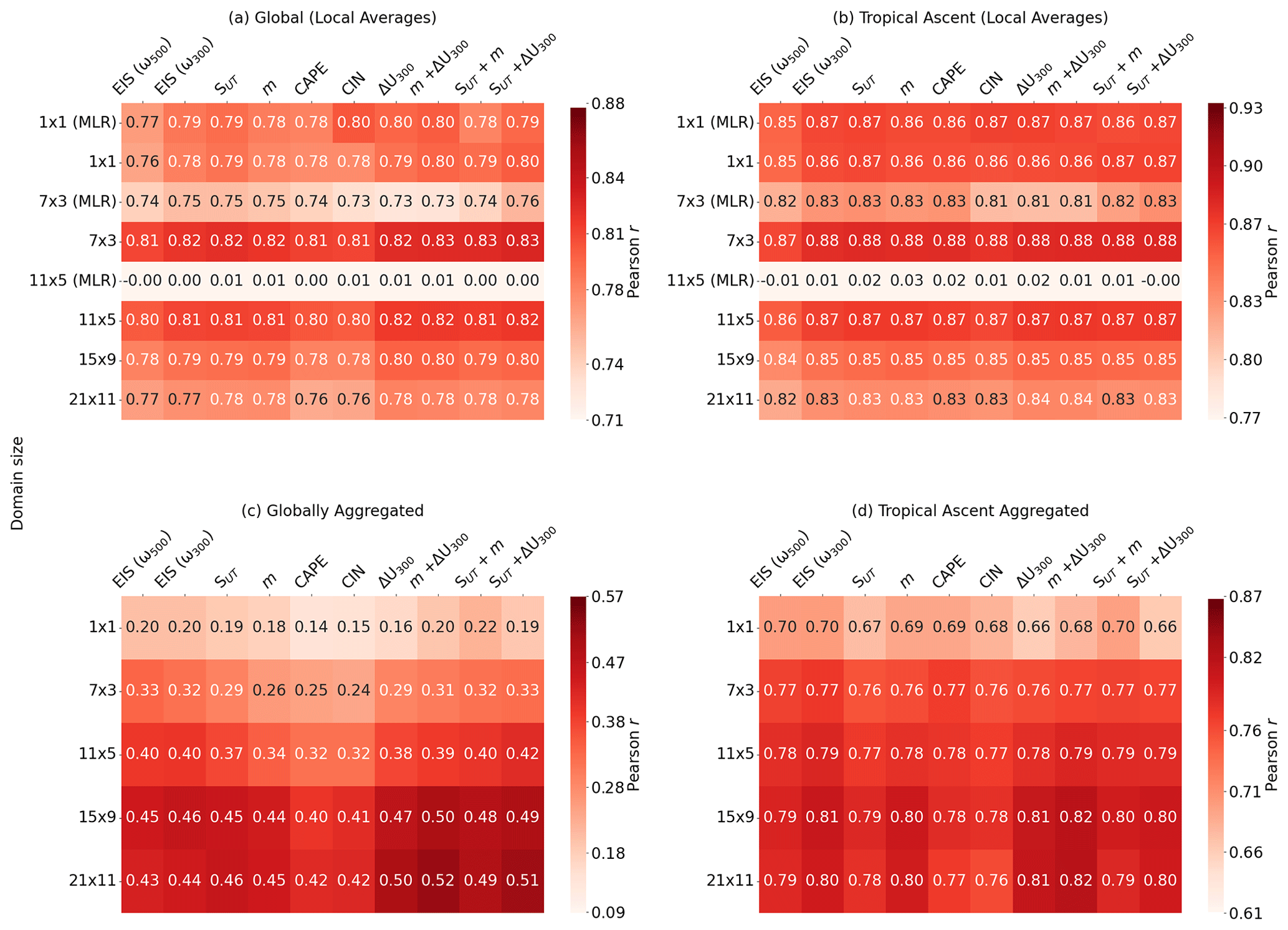
Figure 2Matrices showing Pearson r for predictions made for the observed RLW time series at each domain size using different CCF configurations. A “CCF configuration” refers to the selection of cloud controlling factors used to predict RLW. Each configuration uses Tsfc, RH700, UTRH, and ω300 (with the exception of the first column, where ω500 is used instead) and a candidate CCF (or CCFs) (e.g., SUT), which is used to label each column. Predictions are made locally, with the Pearson r averaged (a) globally and (b) in tropical ascent regions defined as grid cells with observed climatological EIS < 1 K and ω500 < 0 hPa s−1. Metrics are weighted by the cosine of latitude and monthly standard deviation of RLW of each grid cell (see Sect. S2). Pearson r is also shown for aggregated predictions, (c) globally and (d) in the tropical ascent regions, and compared to similarly aggregated observations. All predictions are made using ridge regression, except for rows 1×1 (MLR), 7×3 (MLR), and 11×5 (MLR) in panels (a) and (b), which are made using multiple linear regression. Note different scales for each color bar.
Using the CCF framework, an observational constraint on global cloud feedback can be made using local RLW predictions under a forcing (such as 4xCO2) that are aggregated globally and normalized by the change in global mean surface temperature. Though we do not predict feedback here, we instead assess which CCF configuration best estimates the globally aggregated RLW by spatially averaging each local prediction and target value globally (and in tropical ascent regions) first and then calculating the performance metrics. Henceforth, note a distinction between globally averaged metrics for local predictions (e.g., Fig. 2a–b) and metrics for globally aggregated RLW (e.g., Fig. 2c–d).
5.1 Predictive skill on observations
We first assess CCF configuration skill for local predictions, with results shown in Fig. 2a–b (with columns c–d showing globally aggregated results). Using ridge regression, we confirm that all configurations predict out-of-sample local RLW well at all domain sizes (with correlation matrices qualitatively consistent using R2 and RMSE, not shown). To demonstrate the strengths of ridge regression while using collinear predictors in high dimensions, we briefly compare our results to the traditional multiple linear regression (MLR) approach. Using a 1×1 domain, there is little difference in skill between predictions made with MLR and ridge regression. Beyond 7×3, MLR coefficients become unstable, resulting in predictions that are not correlated with the observed results (e.g., 11×5; results for larger domain sizes are not shown).
We find local performance only slightly depends on the CCF configuration, with EIS (ω500) exhibiting the weakest performance (note that EIS (ω500) is the configuration used in CN21). This is likely because a large proportion of the monthly variability is already explained using only Tsfc, ω300, RH700, and UTRH without the inclusion of additional CCFs (i.e., for 7×3, R2= 0.64 using core CCFs, compared with R2= 0.69 using EIS (w300) in addition). Though changes in local skill (when globally averaged) between the CCF configurations are subtle, we find qualitatively consistent results for the CMIP models, reaffirming that changes are robust. Predictive skill is instead more dependent on domain size, with metrics peaking at the 7×3 domain. We investigate this dependency on domain size in more detail in Sect. 5.1.1.
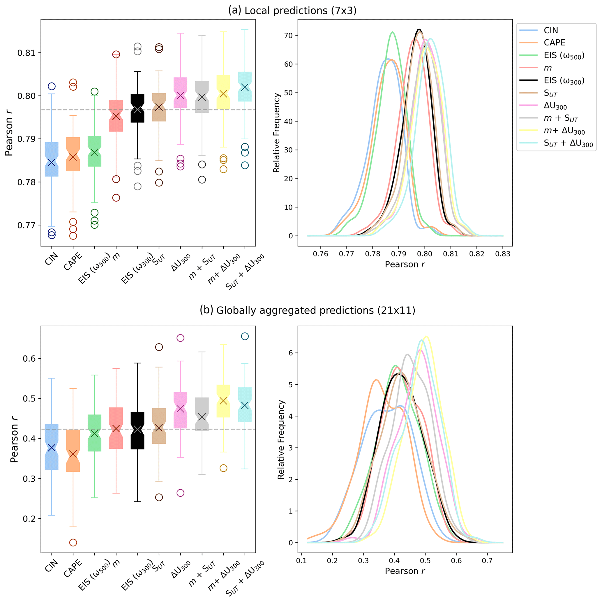
Figure 3Box and whisker plots (left panels) showing the distribution of observed predictive skill based on 100 bootstrapped samples of RLW for a selection of the CCF configurations. Crosses show the means, notches show the medians, and circles show the outliers. A “CCF configuration” refers to the selection of cloud controlling factors used to predict RLW, where each configuration uses Tsfc, RH700, UTRH, and ω300 (with the exception of the first box and whisker, where ω500 is used instead) and a candidate CCF(s) (e.g., SUT), which is used to label each configuration. The right panels show the shapes of the distributions using a kernel density estimator. The top panels (a) show the distributions for local predictions at the 7×3 optimal domain size (analogous to Fig. 2a), and the bottom panels (b) show the distributions for the 21×11 globally aggregated optimal domain size (analogous to Fig. 2c). EIS (ω300) is highlighted in black to facilitate easier comparison between configurations.
In line with Andersen et al. (2023) (though note high-cloud radiative anomalies are not isolated in their study), we find the single largest improvement in RLW predictive skill is achieved through changing ω from 500 to 300 hPa, reflected by a large positive shift in the distributions shown in Fig. 3a. This suggests ω300 more effectively predicts deep convective and cirrus cloud radiative effects than ω500, as we would expect (Ge et al., 2021). We do find that this results in a slight drop in performance for RNET (Fig. S3); this is likely because 500 hPa instead better targets midlevel clouds, which drive a shortwave contribution to RNET that is not present for RLW. However, comparing across configurations using the same vertical velocity reveals qualitatively similar heatmaps for RNET and RLW (note m performs slightly better for RNET than RLW). An additional prominent shift to the distribution arises through the inclusion of ΔU300.
Given that raising the vertical pressure velocity results in a strong positive shift, we henceforth choose to replace ω500 with ω300 and compare further candidate CCF configurations with EIS (ω300) as a new baseline for comparison (highlighted in black in Fig. 3). At the optimal 7×3 domain, we find configuration SUT+ ΔU300 to reproduce observed local RLW with the highest skill, and we hence show the spatial distributions for predictive skill in Fig. S4.
To quantify whether differences between configurations are statistically significant for the observed anomalies, we generate a distribution of Pearson r values using bootstrapping (Davison and Hinkley, 1997). We randomly sample the observed data (with replacement) 100 times, creating datasets equivalent in length to 18 years. Any remaining months are used as a validation dataset, where r is determined against predicted values. This process results in a distribution of 100 r values for each configuration, providing an estimate of predictive skill uncertainty, with a selection of the configurations shown in Fig. 3. The non-parametric Kruskal–Wallis test is hence used to identify statistical differences between all of the distributions. We find highly significant differences between all of the configurations (). Accounting for its highest global median r, we pairwise-test the predictive skill distribution for SUT+ΔU300 with all other configurations (using an adjusted significance level of 0.5 % to account for multiple hypothesis testing). We find statistical similarity with only m+ΔU300 and ΔU300 (p=0.06 and p=0.01, respectively).
We now focus on predictive performance for the globally aggregated RLW time series, with results shown in Figs. 2c–d and 3b. While local prediction performance peaks at 7×3 and is followed by a drop in skill, we find a discrepancy with the globally aggregated performance, which instead increases with domain size. For some configurations, r continues to increase beyond 21×11, though this begins to tail off (not shown). The relationship between domain size and predictive skill now aligns with the findings of CN21, where they show that the correlation between observed and predicted global cloud feedback increases with domain size. However, as domain size increases, so too do the model dimensions and thus the complexity. Owing to the trade-off between small improvements at even larger domain sizes and increased complexity, we restrict our analysis to 21×11 and below and discuss globally aggregated results using the 21×11 domain.
Here we find more marked improvements in predictive skill for most of the CCF configurations compared to EIS (ω500), with performance again strongly dependent on domain size (Fig. 2c–d). However, we now find that changing the pressure level of ω no longer results in a substantial positive shift in the skill distributions, though inclusion of ΔU300 still results in improvements (Fig. 3b). We also note that performance metrics for globally aggregated RLW are comparatively worse than the globally averaged local metrics. This is in line with accumulation of local errors and reduced variability in the globally aggregated anomalies. In a comparison of all globally aggregated distributions shown in Fig. 3b, there is evidence showing statistical differences at the 5 % significance level (with ). Here, m+ ΔU300 has the highest median r. In a pairwise comparison of m+ΔU300 with each other distribution, we find statistical differences with all configurations except SUT+ΔU300 (p=0.02) and ΔU300(p=0.03), again using an adjusted 0.5 % significance level owing to multiple statistical tests.
Neither CAPE nor CIN improves predictive skill at either scale compared to alternative candidate CCFs for most domain sizes. CAPE and CIN have been included as a CCF for their links to deep convection, which is not frequent outside of the warm tropics, resulting in their being particularly poor predictors in the high-latitude extratropics (Fig. S4; for CMIP see Fig. S5). Additionally, the literature hints at a potentially nonlinear relationship between CAPE, CIN, and high cloudiness that would not be captured by the linear ridge regression. For example, in high-CAPE environments it is thought that there may generally be enough CAPE for convection to occur, indicating that the exact magnitude of CAPE is less important than passing a threshold for the onset of deep convection (Sherwood, 1999). The distribution of predictive skill also suggests there is a more complex relationship between CAPE (and CIN, not shown) and RLW. Given that the distributions are calculated using randomly resampled datasets through bootstrapping with replacement, data points will be repeated. This reduces the diversity of the training data, which can result in the poorer generalization of more complex or noisy relationships.
5.1.1 CCF importance at different spatial scales
We investigate the evolution of predictive skill with domain size for locally and globally aggregated predictions. Owing to the linearity of ridge regression, we can partition the predicted local RLW signal into contributions from each CCF, such that (for example)
where is the component of RLW predicted using only Tsfc within the specified domain size and so on for each CCF in the configuration. For each CCF, we calculate the explained variance fraction (EVF) for RLW at each grid cell. Equation (6) is repeated for the global RLW predictions, where local predictions are first globally aggregated for each CCF and then summed. CCFs with higher EVFs are referred to as more “important” for the predicted values (i.e., UTRH is typically the most important predictor for both locally and globally aggregated predictions; shown in Fig. 4). Note that it is plausible that this may show bidirectional causality, where the presence of high cloud influences UTRH by modulating the moisture content in the upper troposphere (i.e., outflow from convective anvils), though our analysis cannot separate the direction.
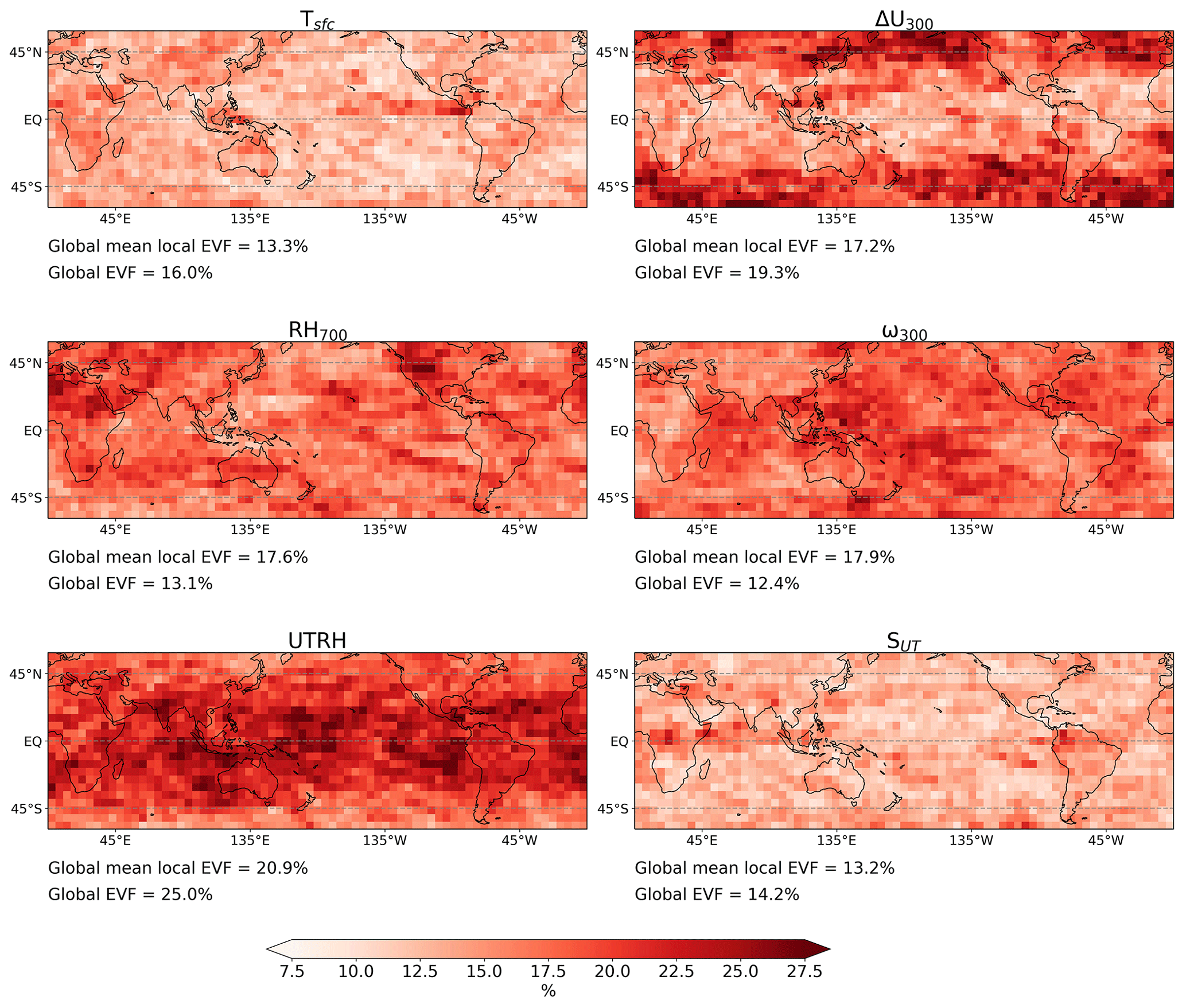
Figure 4Maps showing the explained variance fraction (EVF) as a percentage for local predictions of RLW using a 21×11 domain and using configuration S+ΔU300 (with Tsfc, RH700, UTRH, and ω300). “Global mean local EVF” refers to the global mean EVF from local predictions, weighted by the cosine of each grid cell's latitude. “Global EVF” refers to the EVF for each CCF's contribution to the globally aggregated RLW.
The interaction between domain size, cloud controlling factors, and predictive skill is complex. We summarize key points below:
-
There is an emergent distinction between “local” and “non-local” predictors. For example, EVF for UTRH decreases with increasing domain size, and, accordingly, we find that local UTRH sensitivities typically have strong magnitudes close to the target grid cell, with noisy, spatially incoherent coefficients further afield (see Fig. S6a–b for an example); thus, we describe UTRH as a local CCF (similarly for ω300 and RH700).
-
EVF for Tsfc, ΔU300, and SUT increases with domain size (i.e., non-local predictors), and each contributes a greater proportion of the globally aggregated predictions compared to local predictions (Fig. S6c–d).
-
Predictive skill is likely a trade-off between adding relevant information from non-local CCFs while adding superfluous information from local CCFs; i.e., information that is too distant does not provide additional predictive skill, at least to the degree that it would outweigh the corresponding increase in dimensionality of the regression problem.
-
For globally aggregated predictions, ω300 is the least important predictor (compared to the second most important for local predictions), thus explaining why the choice of pressure level of ω is less relevant at global scales (shown in Fig. 4) than locally.
Our first three points involve the interaction between increasing model dimensions and the addition of potentially relevant context provided by the larger spatial domain. We discuss these points in more detail in Sect. S3. Addressing the last point, we note that several studies point to thermodynamic changes dominating over dynamical effects for global cloud feedback, likely because dynamical effects cancel out at sufficiently large scales (Bony et al., 2004; Byrne and Schneider, 2018; Xu and Cheng, 2016). Conversely, thermodynamic and dynamical feedbacks have more comparable importance at more local scales. We find our results broadly analogous to this. The relatively large EVF for ω at local scales (17.9 %, the second highest in Fig. 4) explains why replacing ω500 with ω300 results in a positive shift to the skill distributions (Fig. 3a). In contrast, globally aggregated EVF for ω300 is comparatively smaller (12.4 %, the lowest value in Fig. 4). This points to the cancellation of large-scale dynamically driven signals when globally aggregated, thus explaining why there is little difference between the performance of ω300 and ω500 in Fig. 2c–d despite resulting in a large improvement for a single CCF change at local scales. Finally, given that ω, an important local predictor, cancels out at globally aggregated scales, the non-local predictors – such as Tsfc – contribute a larger proportion of the total predicted RLW, thus explaining – at least in part – the discrepancy between globally aggregated and local anomalies.
5.2 Predictive skill on CMIP models
Now, we briefly present results for the CCF configurations using the CMIP5/6 models. Key questions are whether the CCF approach performs similarly between models and observations and if there are any obvious discrepancies that could point towards the analysis framework being less applicable than in observations. Performance metrics are first calculated locally for each GCM. Independently for each GCM, the means of the local metrics are calculated globally and in tropical ascent regions. The multi-model median result is then taken, with results analogous to Fig. 2a–b shown in Fig. S7a–b. Finally, we aggregate predictions (globally and in tropical ascent regions) independently for each GCM. The predicted globally and tropical-ascent-aggregated time series are compared against the similarly aggregated target values. Again, note a distinction between globally averaged, local performance metrics and globally aggregated RLW throughout this discussion.
The CMIP Pearson r correlation matrices are broadly analogous to the observed results, where general patterns found in Fig. 2 are also present in Fig. S7. We once again find a discrepancy in optimal domain size, with local performance peaking at 7×3 and globally aggregated RLW peaking at 21×11. Differences include higher multi-model median skill metrics compared to the observations, which may be expected due to intrinsic knowledge of the meteorological conditions embedded within the CMIP models. Additionally, suppressed metrics for observed RLW could be caused by slight mismatches between the observed radiative anomalies and the reanalysis meteorological variables. This therefore results in metrics that are more consistent between CCF configurations than for the observed RLW. In addition, smaller differences between configurations may in part be caused by higher metrics in the first place, leaving less room for improvement. We also find that CAPE performs comparatively better for the CMIP models than in the observations. This may be due to the way in which convection is parameterized in GCMs, thus resulting in stronger modeled relationships between cloud radiative anomalies and CAPE than exist in the observations.
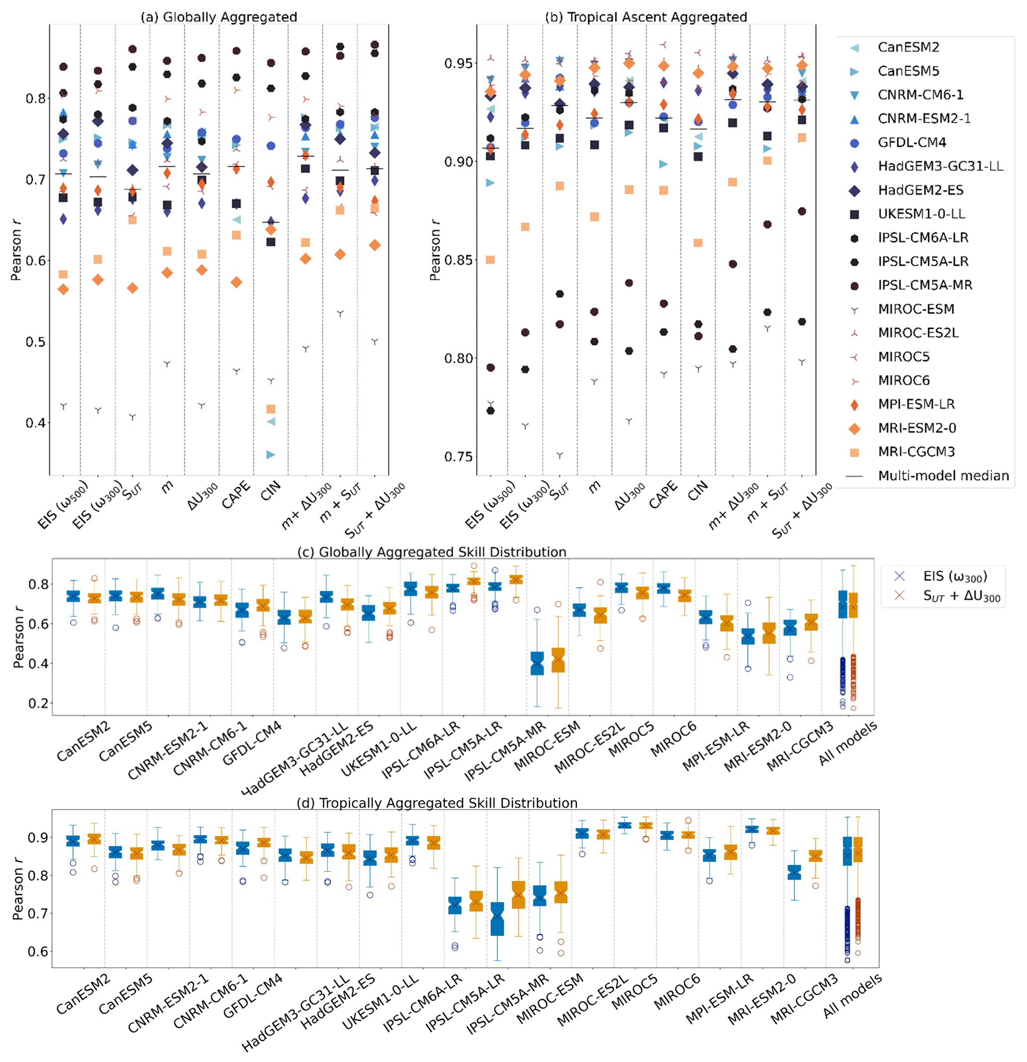
Figure 5Pearson r scores for (a) globally and (b) tropical-ascent-aggregated predictions made at the 21×11 domain size using different CCF configurations. A “CCF configuration” refers to the selection of cloud controlling factors used to predict RLW. Each configuration uses Tsfc, RH700, UTRH, and ω300 (with the exception of the first column, where ω500 is used instead) and a candidate CCF(s) (e.g., SUT). The multi-model median Pearson r is shown from the 14 CMIP models where CAPE and CIN are calculated. The bootstrapped (n= 100) predictive skill distributions for EIS (ω300) and SUT+ΔU300 are shown at the optimal 21×11 domain size for (c) globally aggregated predictions and (d) tropical-ascent-aggregated predictions.
Highlighting uncertainties within the CMIP models themselves, there is a large spread in the skill metrics, shown for aggregated predictions in Fig. 5a–b. We find that changes to the globally aggregated performance do not imply similar changes to the tropical-ascent-aggregated performance. For example, SUT shows a slight decrease in the global multi-model median r compared to EIS (ω300) despite showing a positive shift for predictions aggregated in the tropical ascent regions. Secondly, improvements to the multi-model median r do not imply that each GCM shows improvements independently. For example, the multi-model median r for tropical-ascent-aggregated predictions made using configuration SUT has improved compared to configuration EIS (ω300); models such as MRI-CGCM3, GFDL-CM4, and IPSL-CM5A-MR have large leaps in Pearson r. Conversely, MIROC-ESM, CanESM5, and HadGEM2-ES show decreases. Opposing improvements and deteriorations of predictive skill are partially responsible for the relatively small change in multi-model r between the configurations for the CMIP models.
In Sect. 5.1, we highlighted SUT+ΔU300 as a possible optimal configuration. Here we identify whether differences between the CMIP-modeled predictive skill distributions for EIS (ω300) and SUT+ΔU300 are statistically significant. In a pairwise Kruskal–Wallis test on the combined Pearson r scores from all 18 models (n=1800), we find a significantly higher predictive skill distribution for SUT+ΔU300 than EIS (ω300) with (distributions not shown). This is unsurprising; 15 of the 18 individual CMIP models have a higher median r using SUT+ΔU300 compared with EIS (ω300).
Despite a slightly lower multi-model median, we find that the globally aggregated distributions for all models combined are statistically similar at the 5 % significance level (shown in Fig. 5c; p=0.13). Here, only half of the CMIP models have a higher median r using SUT+ΔU300 compared with EIS (ω300). However, visual inspection of the distributions for predictions aggregated in the tropical ascent regions (Fig. 5d) suggests that improvements found using SUT+ΔU300 instead of EIS (ω300) are more pronounced than any deteriorations. In summary, while the mean evolution of predictive skill within the CMIP models is broadly aligned with the observations, there are nuances which likely depend on the parameterization within the models themselves (Li et al., 2012; Qu et al., 2014; Rio et al., 2019). This leads to a slightly different evolution of predictive skill with the configuration between the CMIP models.
5.3 Physical interpretation of the cloud radiative sensitivities
In addition to the statistical performance metrics, we study the spatial distribution and magnitude of the sensitivities. Interpreting spatial sensitivities can be used in CCF analysis to justify predictor selection that is grounded in physical reasoning and can be done for any of the CCF configurations (e.g., Andersen et al., 2023). Though our analysis has identified two strong configurations, SUT+ΔU300 and m+ ΔU300, we only physically interpret the sensitivities of RLW to the CCFs in configuration SUT+ΔU300 in this section. We choose SUT+ΔU300 over m+ ΔU300 based on the wider literature examining the relationship between high-cloud occurrence and static stability (e.g., Li et al., 2014) and due to the link between static stability and changes in tropical anvil cloud fraction through the “anvil iris” thermodynamic mechanism (Bony et al., 2016; Saint-Lu et al., 2020, 2022). We recommend a similar physical interpretation of sensitivities be performed should alternative configurations be used in similar CCF applications, such as constraining cloud feedback.
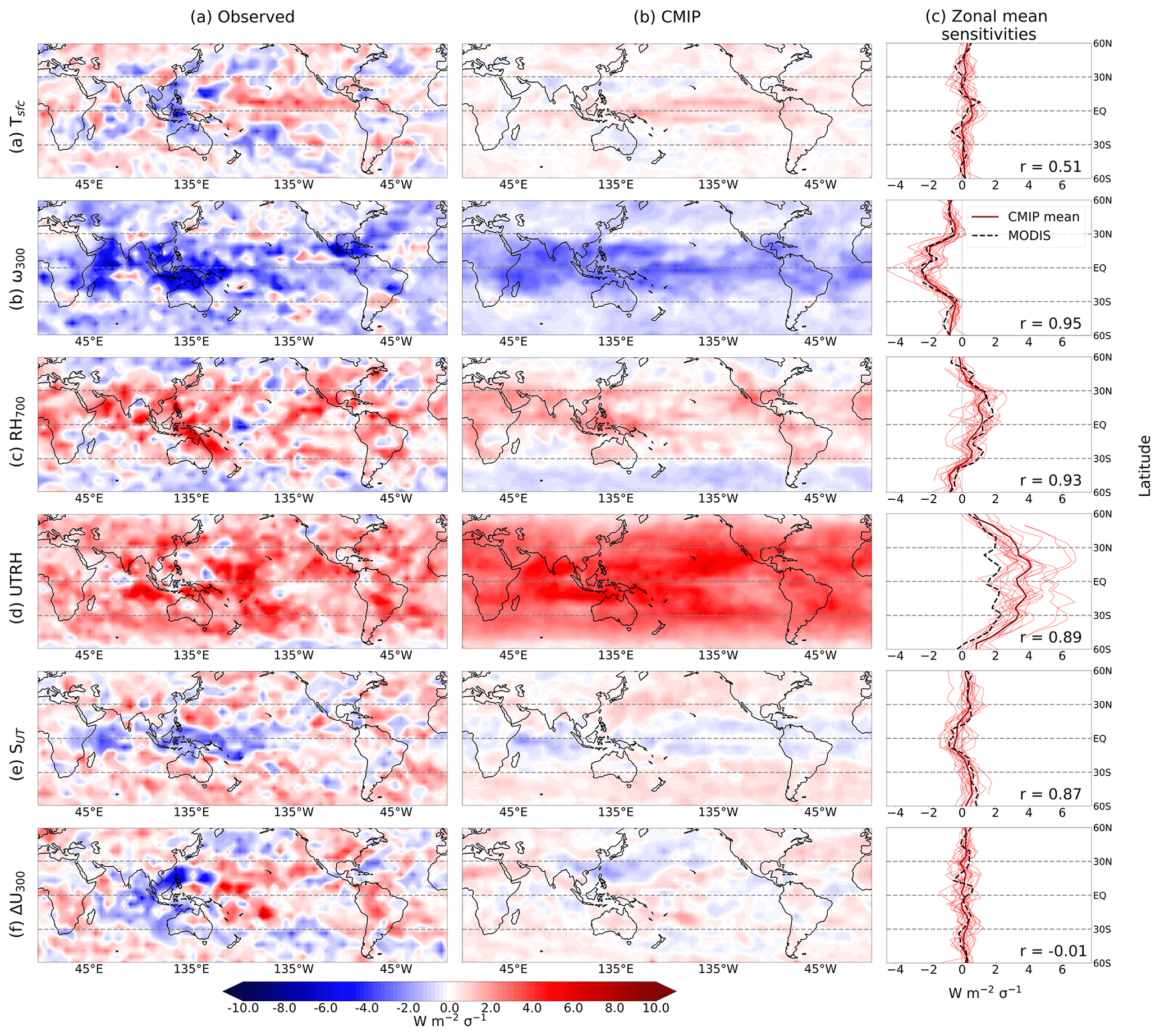
Figure 6RLW sensitivities (∑Θi) to the cloud controlling factors in configuration SUT+ΔU300 (also with Tsfc, RH700, UTRH, and ω300), derived using a 21×11 domain and defined for a 1-standard-deviation anomaly in each CCF (scaled using ERA5 CCFs for visualization purposes). To produce the maps, we sum all elements of the sensitivity vectors at each point r. The column (a) shows observed sensitivities, and column (b) shows the multi-model mean. Column (c) shows zonal average sensitivity for the observations (dashed line), the multi-model mean (dark solid line), and individual CMIP model sensitivities. The Pearson r correlation coefficient for the zonal mean sensitivities is shown in the bottom corner of each panel.
For each CCF in the configuration, we sum each contribution Θi within the entire spatial domain (e.g., Eq. 5 for RLW) and plot the total for each grid cell. This is the spatial sensitivity of the cloud radiative anomaly to a given CCF, normalized for a 1-standard-deviation anomaly. Here, we derive the sensitivities using the full 20-year datasets (with no dataset rotation or bootstrapping). There are several studies interpreting relationships between cloud radiative anomalies and the core CCFs (e.g., CN21; Andersen et al., 2023), though not explicitly for high clouds. Therefore, we first briefly interpret our sensitivities to the core CCFs, shown in Fig. 6a–d. We then assess the sensitivities for cloud properties (i.e., cloud-top pressure and cloud fraction) before interpreting sensitivities for the additional CCFs, SUT+ ΔU300.
The observed and multi-model mean spatial distributions for the core CCFs – Tsfc, ω300, UTRH, and RH700 – broadly align with what we expect and are qualitatively similar between the observations and multi-model means. We note that the observed global median regularization parameter, α, lies towards the upper end of the inter-model spread (not shown). We speculate that the CCFs in the CMIP models typically capture the variability in RLW with greater skill than the observations, meaning less regularization is required on average. For all CCFs except UTRH, the magnitudes of the modeled sensitivities are smaller than the observed results (tropical ascent sensitivities shown in Fig. 7). It is known that (CMIP5) GCMs underestimate the frequency of tropical anvil cloud and extratropical cirrus occurrence (Ceppi et al., 2017; Tsushima et al., 2013) and thus their radiative effects, which can also explain smaller sensitivities on average.
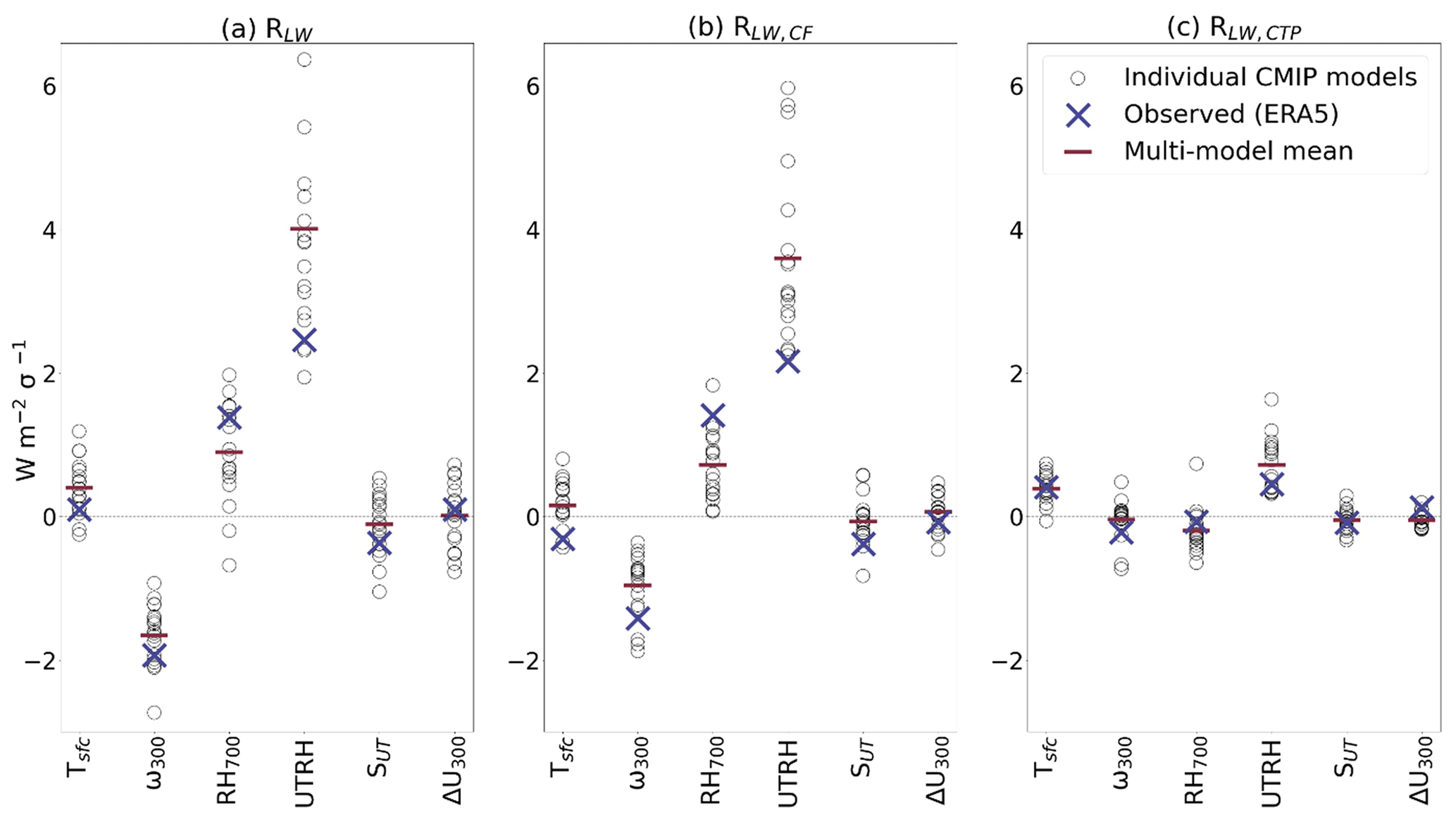
Figure 7Observed and CMIP sensitivities to the cloud controlling factors in configuration SUT+ΔU300 (with Tsfc, RH700, UTRH, and ω300), derived using a 21×11 domain and defined for a 1-standard-deviation anomaly for each CCF, averaged over all tropical ascent grid cells for (a) RLW, (b) RLW,CF, and (c) RLW,CTP. The standard deviation used to scale each CCF has been calculated from the observed CCFs.
The RLW – Tsfc sensitivities (i.e., Eq. 5 summed for all X=Tsfc) shown in Fig. 6a are generally small in magnitude, with regions of positive sensitivity in the central and east Pacific (responsible for a slight positive peak in observed zonal mean sensitivity) and with negative (or, for the CMIP models, reduced magnitude) sensitivity over the Maritime Continent. The RLW – UTRH sensitivities are ubiquitously positive and large in magnitude, consistent with increasing high cloudiness with humidity, though Fig. 6d shows that CMIP-modeled sensitivities are consistently larger in magnitude than what is observed. This is possibly due to stronger coupling between upper-tropospheric humidity and cloud incidence in the CMIP models than in the observations, owing to the parameterization of clouds in the models themselves (Li et al., 2012; Qu et al., 2014). The RH700 sensitivities are also widely positive (though negative at high latitudes), with smaller magnitude than UTRH (as we would expect for high clouds) and with the largest magnitudes in the deep tropics. Indicating increased high cloudiness with increased ascent, the ω300 sensitivities are nearly ubiquitously negative, with the strongest magnitudes broadly aligning with the tropical ascent regions in both observations and the CMIP models.
We use the decomposition of RLW into its linear sum of contributions from changes in cloud-top pressure (CTP), cloud fraction (CF), and optical depth and a small residual (with other components held fixed) to further interpret our sensitivities (Zelinka et al., 2012a, b, 2016). We do not show optical depth sensitivities here, owing to their small role in driving LW high-cloud radiative anomalies (see Fig. S10). LW radiative anomalies caused by changes in the cloud properties are henceforth referred to using an additional subscript; i.e., RLW,CTP is the contribution that changes in cloud-top pressure (with no change in τ or CF) have to the total RLW. Sensitivities for the decompositions can be found in Figs. S8–S9. We average the domain-summed sensitivities in the tropical ascent regions, shown in Fig. 7.
The RLW−Tsfc sensitivities average to approximately zero in the tropical ascent regions for the observations (Fig. 7a) with good agreement globally between the CMIP models and observations (zonal mean r=0.52). Figure 6a shows a distinct positive sensitivity present over the Pacific Ocean, which we ascribe to an increase in high cloud-top pressure that is associated with warming sea surface temperature anomalies, thus radiating heat to space at cooler temperatures. We find that the spatial patterns of sensitivities in the tropics are widespread positive (Fig. S9), as we would expect (though more strongly positive in the models than the observations). Accordingly, the observed sensitivities in the tropical ascent regions are positive, with a larger magnitude than the similarly averaged and opposite-signed sensitivities (Fig. 7). This is despite a much smaller monthly signal for observed RLW,CTP than RLW,CF. The modeled sensitivities are stronger than the counterparts, resulting in the slightly more positive CMIP RLW−Tsfc sensitivities.
The RLW−ΔU300 sensitivity, shown in Fig. 6f, is more challenging to interpret than the core CCFs (Anber et al., 2014). This is partially due to the dynamic nature of wind shear; coefficients within the spatial domain capture dynamic variability signals, which may result in a range of positive and negative sensitivities, therefore being canceled in the summation over the 21×11 domain. There is also less agreement between the observed and multi-model mean spatial distributions than all other CCFs, which may partially be caused by offset circulation cells in the CMIP models, resulting in different local sensitivities and dynamic signals (zonal mean ). Here, we suggest reasons for both positive and negative sensitivities. Over the Maritime Continent and Indian Ocean, observed sensitivities are broadly negative. It is known that wind shear can hasten the dissipation of tropical tropopause cirrus (Jensen et al., 2011), which would result in decreased cloudiness and thus LW cooling. Conversely, there are many regions where the sensitivity is positive (such as the central Pacific), which indicates LW warming with increased shear. This may be a result of shear spreading the high cloud, thus increasing cloud fraction (Lin and Mapes, 2004) and in turn reducing outgoing LW radiation. The role of wind shear may be sensitive to the pressure level relative to the tropopause (Chakraborty et al., 2016; Nelson et al., 2022). Given that we use the same shear height (i.e., the difference in 300 and 925 hPa wind speeds) globally, it is likely that the zonal distribution of tropopause heights may cause the differing relationships. Despite differences between the spatial distributions, both observed and the multi-model mean sensitivities in the tropical ascent regions are consistent with each other and average to approximately zero. We suspect this may due to shear being important for the organization of convection, which is not represented in GCMs.
Finally, we address the SUT sensitivities. Both the observed and multi-model mean RLW−SUT sensitivities, shown in Fig. 6e, are predominantly negative in the tropics, with the largest magnitudes over the central and west Pacific and Maritime Continent (though more markedly so for the observations). Therefore, in the absence of changes in the other CCFs, anomalies in high cloud associated with an increase in SUT would result in increased longwave emission to space over the tropics. This is what we expect, given the negative relationship between upper-tropospheric cloud incidence and static stability over tropical oceans (Li et al., 2014).
The observed sensitivities are negative across the tropics – most strongly in regions with high RLW,CF signals (see Fig. S8). This reveals that LW cooling arises – at least in part – from a reduction in high-cloud fraction, qualitatively resembling the anvil iris mechanism (Bony et al., 2016; Saint-Lu et al., 2020). As anvil clouds rise in response to global warming, their environment becomes more stable, owing to the dependency of static stability on atmospheric pressure (Saint-Lu et al., 2020, 2022). In a more stable atmosphere, the vertical pressure gradient associated with subsidence in clear-sky conditions is reduced. Owing to mass conservation, a reduction in the subsidence pressure gradient results in a reduction in anvil cloud fraction, caused by a decrease in horizontal convergence (Saint-Lu et al., 2020, 2022).
We find that the mean CMIP RLW−SUT sensitivity in the tropical ascent regions is smaller in magnitude than the observed results, with considerable disagreement in sign (ranging from −1.0 to 0.44 W m; Fig. 7a). Most of the total RLW−SUT sensitivity arises from the CF component (Fig. 7b), where the CMIP model mean approaches zero, though with a similarly large range. Though it is thought to be small in magnitude, the anvil cloud area feedback is subject to much uncertainty and underestimated by GCMs (Zelinka et al., 2022), consistent with our results. CMIP models are known to predict a wide range of anvil cloud fraction feedbacks, including “unlikely” very positive feedback (Zelinka et al., 2022), which is perhaps reflected by strong positive tropical RLW−SUT sensitivities for two GCMs (Fig. S8e). Given that static stability has been shown to robustly control high-cloud fraction (Saint-Lu et al., 2022), and based on our results, we propose that the addition of SUT into observational constraint frameworks may reduce some of the uncertainty arising from the anvil fraction feedback.
We also find that the spatial distributions for the observed and multi-model mean sensitivities are broadly similar with zonal mean correlation r=0.60. For observations, the sensitivity is negative in the west Pacific and Maritime Continent, indicating that an increase in SUT results in LW cooling, arising from a change (i.e., a decrease) in cloud-top pressure. Increased static stability results in suppressed vertical motion, which in turn prevents cloud tops from rising as high as they might in a more unstable environment (Saint-Lu et al., 2022; Zelinka and Hartmann, 2010, 2011). Negative sensitivities in the tropical ascent regions are less prevalent for the models, with negative sensitivities more widespread in the subtropics. This results in a smaller magnitude of the CMIP sensitivities in the tropical ascent regions (Fig. 7c).
As well as absorbing upwelling LW radiation, high clouds can reflect incident SW radiation depending on their optical depth. While RLW (and thus the sensitivities) is primarily driven by CF and CTP changes, RNET is also driven by changes in optical depth, which predominantly affects SW radiative anomalies that we have not directly assessed. Thus, the net high-cloud radiative anomaly is comprised of complex interplay between competing LW and SW effects. The magnitude of the observed RNET−SUT sensitivity is much smaller than the RLW−SUT component in the tropical ascent regions, though the spatial distribution is broadly similar (Fig. S11) and negative in many high-cloud regions. This suggests that, assuming an increase in SUT with warming (Bony et al., 2016), high clouds exert a negative (though weak) net feedback. However, the observed CMIP mean tropical ascent sensitivities average to approximately zero, indicating a very weak anvil cloud area feedback with increasing SUT. While a weak anvil cloud feedback may be expected (McKim et al., 2024), it is also thought CMIP models tend to underestimate a negative anvil cloud fraction feedback (Zelinka et al., 2022). Additionally, Zelinka et al. (2022) show that eight CMIP models (including six of those used in this research) predict an “unlikely” positive feedback arising from changes in anvil cloud fraction. Therefore, the near-zero multi-model sensitivities may also arise due to cancellation of local sensitivities between the models.
5.4 Predicting radiative anomalies from cloud fraction and cloud-top pressure changes
Based on the physical interpretation of the sensitivities, our results – combined with the previous literature and theory – thus far support the use of SUT+ΔU300 in high-cloud controlling factor frameworks. We have shown that SUT+ΔU300 reproduces the locally and globally aggregated RLW with high skill for observations and performs well for the CMIP models. Additionally, the sensitivities shown in Fig. 6 suggest that the mechanisms driving high-cloud feedback – rising free-tropospheric clouds and reduction in anvil cloud fraction (Ceppi et al., 2017) – are captured by this selection of CCFs at the 21×11 domain. Finally, we question whether our approach captures the spatial pattern, temporal variability, and magnitude of these properties.
We predict 20 years of cloud radiative anomalies induced by CF and CTP changes (with other components held fixed) for both observations and CMIP models, again using rotating 18-year datasets. We globally aggregate the predicted anomalies (e.g., as in Fig. 2c) and compare against similarly aggregated target values using the Pearson r correlation coefficient. We do not assess optical-depth-induced changes, owing to their small historical LW signal (see Fig. S10). Though optical depth is important for historical SW (and consequently net) radiative anomalies, the high-cloud optical depth feedback is thought to be relatively small (Zelinka et al., 2022), and so we focus on CF and CTP. We place particular emphasis on the observations here, as the El Niño phase of the El Niño–Southern Oscillation (ENSO) from July 2015 to June 2016 saw anomalous warming in the east Pacific (see Fig. 8, top panel). ENSO is a dominant driver of natural ocean–atmosphere variability, resulting in regional tropical temperature and circulation anomalies that are accompanied by changes in cloud properties and the TOA radiation budget (Ceppi and Fueglistaler, 2021). Accordingly, July 2015 to June 2016 has one of the most anomalously warm annual mean surface temperatures in the 20-year record. We only highlight this El Niño event for the observed cloud properties, as it will be absent from the coupled historical simulations, and Atmospheric Model Intercomparison Project (AMIP) simulations do not reach 2016.
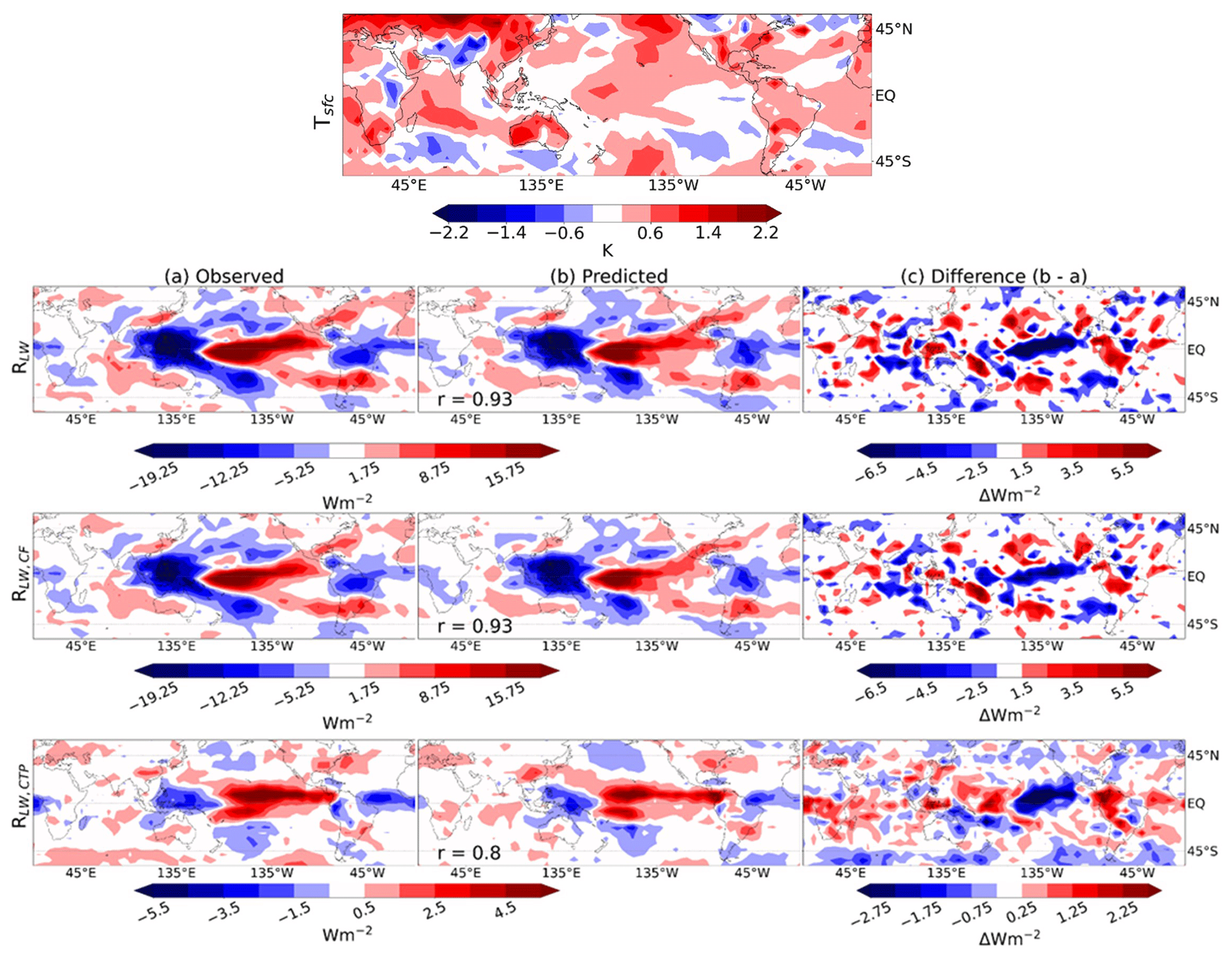
Figure 8Observed mean El Niño surface temperature anomaly (top) and radiative anomalies (a), averaged from July 2016–June 2015 relative to the full 20-year record. Predicted anomalies (b) made using a 21×11 domain and the configuration SUT+ΔU300 (with Tsfc, RH700, UTRH, and ω300) for the El Niño months. The difference (predicted minus observed) is shown in panel (c). The Pearson r spatial correlation between (a) and (b) is shown in the bottom left of panel (b). Note different color bar ranges.
Out-of-sample globally aggregated RLW,CF is well predicted by configuration SUT+ΔU300 with a correlation coefficient of 0.63. The spatial distribution of the El Niño CF anomalies closely follows the RLW distribution owing to its large signal and is reproduced accurately with a correlation coefficient of r = 0.93 (Fig. 8). There is a positive RLW,CF anomaly in the east Pacific, overlapping the region of anomalous sea surface warming, indicating increased cloud fraction. Warmer SSTs enhance convection, resulting in increased upward motion and thus increased high cloudiness. In the west Pacific, the SST anomaly is negative and smaller in magnitude, though there is a strong, negative RLW,CF anomaly, indicating a reduction in cloud fraction. Owing to the shift in circulation, suppressed convection can result in anomalous subsidence, hence reducing high cloudiness. Our configuration predicts RLW,CF with slight negative error in the east Pacific, indicating an underestimation of the increased cloud fraction. In the west Pacific, where there is an observed reduction in cloud fraction, our predictions have little error.
We also predict observed, globally aggregated RLW,CTP well, though with slightly reduced correlation coefficients compared to RLW,CF (r=0.68). Figure 9b shows that the magnitudes of strong positive and negative anomalies are slightly underestimated; this may be caused by a small signal for the regression model to learn from (see Fig. S10). Alternatively, this may hint towards a nonlinear relationship between cloud-top pressure and the CCFs, which would not be captured by ridge regression and (in addition to CCF selection) could explain poorer skill for predicting LW cloud feedback (CN21). Regardless, the spatial distribution of predicted El Niño RLW,CTP is again strongly correlated to the observed results, here with r= 0.80 (Fig. 9a). Strong positive anomalies are present over the east Pacific, which we ascribe to a rise in cloud-top pressure due to enhanced convection. As the atmosphere warms, a shift in the RLW,CTP distribution towards higher values, particularly in the tropics, may be expected owing to the rising of free-tropospheric clouds (Ceppi et al., 2017). We note that the globally aggregated, annual mean RLW,CTP during this El Niño event is the most extreme positive anomaly in the observed 20-year record and is reproduced with small absolute error (−0.01 W m−2). Accordingly, we predict the most positive RNET,CTP annual anomaly with similarly small absolute error and correlation coefficient (absolute error −0.01 W m−2, r=0.57; see Fig. S12). This is consistent with the extreme warmth during that period and the associated rise of the tropopause. Despite potentially underestimating the amplitude of the monthly variability, our method does an excellent job capturing the most extreme (positive) annual anomaly out-of-sample (Fig. 9b). We also find that configurations SUT and SUT+ΔU300 predict the tropical mean El Niño RLW,CTP with the smallest absolute error (not shown).
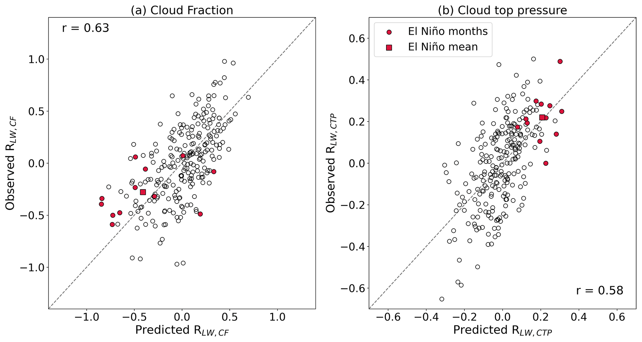
Figure 9Scatter plot showing the correlation between observed and predicted monthly globally aggregated (a) RLW,CF and (b) RLW,CTP time series using configuration SUT+ΔU300 (in addition to Tsfc, RH700, UTRH, and ω300) and a 21×11 domain. El Niño months are shown using colored circles, with the annual mean shown using a colored square. Solid lines show y=x, and the dashed lines show the line of best fit through the points. For RNET,CF and RNET,CTP, see Fig. S12.
We additionally confirm that our framework predicts out-of-sample globally aggregated RLW,CF and RLW,CTP with good skill in the CMIP models, once again with slightly higher correlation coefficients than the observed results (multi-model medians of r=0.75 and 0.77, respectively). To summarize, we have shown that the spatial distributions of the observed El Niño anomalies are captured well, including the most extreme positive RLW,CTP annual anomaly, thus highlighting the strength of our proposed configuration SUT+ΔU300. We reiterate that the SUT sensitivities (Figs. 6e, S8e–S9e) are physically congruent with the previous literature and appear to directly target the drivers of high-cloud feedback.
Few studies directly assess cloud controlling factors for high clouds despite their substantial contributions to cloud feedback. Here, a selection of candidate cloud controlling factors (CCFs) have been used to predict high-cloud radiative anomalies using ridge regression. We investigate five candidate CCFs – static stability in the upper troposphere, sub-cloud moist static energy, wind shear, convective available potential energy, and convective inhibition – using the additional “core” meteorological drivers of surface temperature, lower- and upper-tropospheric relative humidity, and upper-tropospheric vertical pressure velocity in each configuration. CCFs are used within a two-dimensional spatial domain to predict out-of-sample longwave cloud radiative anomalies, RLW. We assess configurations from local to globally aggregated spatial scales and physically interpret the spatial distribution of the sensitivities for the configuration SUT+ΔU300. Finally, we assess the skill of SUT+ΔU300 for predicting out-of-sample anomalies induced by changes in cloud-top pressure and cloud fraction, including the El Niño event of 2015–2016.
We find that the optimal domain size and CCF combination are dependent on the temporal and spatial scales assessed, and we summarize the most relevant findings here:
-
All configurations predict out-of-sample historical variability for RLW (and RNET) with good skill for observations and CMIP models at local scales. A domain of 7×3 optimizes local predictions, where we show that ridge regression skill surpasses traditional multiple linear regression.
-
Conversely to local predictions, predictive skill for globally aggregated (i.e., a global spatial average) radiative anomalies increases with domain size, peaking at 21×11. We suggest a trade-off between local and non-local predictors is partially responsible for this domain size discrepancy between local and global predictions, though unraveling this remains a key question for future research.
-
The main mechanisms driving high-cloud feedback – rising of free-tropospheric clouds and reduction in anvil cloud fraction – appear to be captured by the core and candidate CCFs in the SUT+ ΔU300 configuration. The spatial distributions of the RLW sensitivities to the core CCFs and SUT are physically consistent with our understanding and expectations, with observed and CMIP-modeled sensitivities qualitatively similar. There are larger differences between observed and the multi-model mean ΔU300 sensitivities, which are more complex to interpret than the core CCFs and SUT.
-
Out-of-sample globally aggregated anomalies induced by cloud-top pressure and cloud fraction changes are predicted well using SUT+ΔU300 in both observations and models. In particular, we obtain a quantitatively accurate out-of-sample prediction of the observed extreme anomalies in , and RLW,CTP during the 2015–2016 El Niño. The corresponding spatial distributions are also predicted with high correlation coefficients (r≥0.80).
Our systematic evaluation of high-cloud controlling factors highlights SUT+ΔU300 as a possible optimal configuration for CCF frameworks. Of course, our work is only the first attempt to assess candidates for high-cloud controlling factors so we welcome future work on additional candidate factors that might not have been considered here. We have also identified an important inconsistency regarding ideal domain size for CCF predictions on historical data locally and globally aggregated. Given the strong out-of-sample predictive power of our framework, in future work we will use our optimal CCF configurations to constrain high-cloud feedback.
ERA5 meteorological reanalysis data are freely available from the Copernicus Climate Change Service (C3S) Climate Data Store (https://doi.org/10.24381/cds.f17050d7, Hersbach et al., 2023a; https://doi.org/10.24381/cds.6860a573, Hersbach et al., 2023b; and https://doi.org/10.24381/cds.bd0915c6, Hersbach et al., 2023c). Combined MODIS Aqua–Terra data are also freely available and downloaded monthly (https://doi.org/10.5067/MODIS/MCD06COSP_M3_MODIS.062, Hubanks et al., 2022). All CMIP5/6 data were obtained from the UK Center for Environmental Data Analysis portal (https://esgf-ui.ceda.ac.uk/cog/projects/esgf-ceda/, CEDA, 2024).
The supplement related to this article is available online at: https://doi.org/10.5194/acp-24-8295-2024-supplement.
SWK, PN, and PC conceptualized this research. SWK conducted the analysis and wrote the first draft of this article. SWK, PC, PN, HA, JC, and PS each contributed towards the interpretation of the results. PC, PN, HA, JC, and PS all provided critical feedback on the draft and final manuscript.
At least one of the (co-)authors is a member of the editorial board of Atmospheric Chemistry and Physics. The peer-review process was guided by an independent editor, and the authors also have no other competing interests to declare.
Publisher’s note: Copernicus Publications remains neutral with regard to jurisdictional claims made in the text, published maps, institutional affiliations, or any other geographical representation in this paper. While Copernicus Publications makes every effort to include appropriate place names, the final responsibility lies with the authors.
Firstly, we would like to thank the two anonymous reviewers for thoughtful and helpful comments which have improved this paper. This research was carried out on the High Performance Computing Cluster supported by the Research and Specialist Computing Support service at the University of East Anglia and additionally JASMIN, the UK's collaborative data analysis environment (https://jasmin.ac.uk, last access: 17 July 2024).
This research has been supported by the Natural Environment Research Council (grant no. NE/V012045/1), the European Horizon 2020 (grant no. 821205), and the Deutsche Forschungsgemeinschaft (grant no. 440521482).
This paper was edited by Minghuai Wang and reviewed by two anonymous referees.
Anber, U., Wang, S., and Sobel, A.: Response of Atmospheric Convection to Vertical Wind Shear: Cloud-System-Resolving Simulations with Parameterized Large-Scale Circulation. Part I: Specified Radiative Cooling, J. Atmos. Sci., 71, 2976–2993, https://doi.org/10.1175/JAS-D-13-0320.1, 2014.
Andersen, H., Cermak, J., Fuchs, J., Knutti, R., and Lohmann, U.: Understanding the drivers of marine liquid-water cloud occurrence and properties with global observations using neural networks, Atmos. Chem. Phys., 17, 9535–9546, https://doi.org/10.5194/acp-17-9535-2017, 2017.
Andersen, H., Cermak, J., Zipfel, L., and Myers, T. A.: Attribution of Observed Recent Decrease in Low Clouds Over the Northeastern Pacific to Cloud-Controlling Factors, Geophys. Res. Lett., 49, e2021GL096498, https://doi.org/10.1029/2021GL096498, 2022.
Andersen, H., Cermak, J., Douglas, A., Myers, T. A., Nowack, P., Stier, P., Wall, C. J., and Wilson Kemsley, S.: Sensitivities of cloud radiative effects to large-scale meteorology and aerosols from global observations, Atmos. Chem. Phys., 23, 10775–10794, https://doi.org/10.5194/acp-23-10775-2023, 2023.
Bodas-Salcedo, A., Webb, M. J., Bony, S., Chepfer, H., Dufresne, J.-L., Klein, S. A., Zhang, Y., Marchand, R., Haynes, J. M., Pincus, R., and John, V. O.: COSP: Satellite simulation software for model assessment, B. Am. Meteorol. Soc., 92, 1023–1043, https://doi.org/10.1175/2011BAMS2856.1, 2011.
Bony, S., Lau, K.-M., and Sud, Y. C.: Sea Surface Temperature and Large-Scale Circulation Influences on Tropical Greenhouse Effect and Cloud Radiative Forcing, J. Climate, 10, 2055–2077, https://doi.org/10.1175/1520-0442(1997)010<2055:SSTALS>2.0.CO;2, 1997.
Bony, S., Dufresne, J.-L., Le Treut, H., Morcrette, J.-J., and Senior, C.: On dynamic and thermodynamic components of cloud changes, Clim. Dynam., 22, 71–86, https://doi.org/10.1007/s00382-003-0369-6, 2004.
Bony, S., Stevens, B., Coppin, D., Becker, T., Reed, K. A., Voigt, A., and Medeiros, B.: Thermodynamic control of anvil cloud amount, P. Natl. Acad. Sci. USA, 113, 8927–8932, https://doi.org/10.1073/pnas.1601472113, 2016.
Bretherton, C. S.: Insights into low-latitude cloud feedbacks from high-resolution models, Philos. T. R. Soc. A, 373, 20140415, https://doi.org/10.1098/rsta.2014.0415, 2015.
Brient, F. and Schneider, T.: Constraints on Climate Sensitivity from Space-Based Measurements of Low-Cloud Reflection, J. Climate, 29, 5821–5835, https://doi.org/10.1175/JCLI-D-15-0897.1, 2016.
Byrne, M. P. and Schneider, T.: Atmospheric Dynamics Feedback: Concept, Simulations, and Climate Implications, J. Climate, 31, 3249–3264, https://doi.org/10.1175/JCLI-D-17-0470.1, 2018.
CEDA: ESGF Portal, https://esgf-ui.ceda.ac.uk/cog/projects/esgf-ceda/ (last access: 18 July 2024), 2024.
Ceppi, P. and Fueglistaler, S.: The El Niño–Southern Oscillation Pattern Effect, Geophys. Res. Lett., 48, e2021GL095261, https://doi.org/10.1029/2021GL095261, 2021.
Ceppi, P. and Nowack, P.: Observational evidence that cloud feedback amplifies global warming, P. Natl. Acad. Sci. USA, 118, e2026290118, https://doi.org/10.1073/pnas.2026290118, 2021.
Ceppi, P., Brient, F., Zelinka, M. D., and Hartmann, D. L.: Cloud feedback mechanisms and their representation in global climate models, WIREs Climate Change, 8, e465, https://doi.org/10.1002/wcc.465, 2017.
Chakraborty, S., Fu, R., Massie, S. T., and Stephens, G.: Relative influence of meteorological conditions and aerosols on the lifetime of mesoscale convective systems, P. Natl. Acad. Sci. USA, 113, 7426–7431, https://doi.org/10.1073/pnas.1601935113, 2016.
Chen, T., Rossow, W. B., and Zhang, Y.: Radiative Effects of Cloud-Type Variations, J. Climate, 13, 264–286, https://doi.org/10.1175/1520-0442(2000)013<0264:REOCTV>2.0.CO;2, 2000.
Davison, A. C. and Hinkley, D. V.: Bootstrap Methods and Their Application, Cambridge University Press, 606 pp., https://doi.org/10.1017/CBO9780511802843, 1997.
Donner, L. J. and Phillips, V. T.: Boundary layer control on convective available potential energy: Implications for cumulus parameterization, J. Geophys. Res.-Atmos., 108, 4701, https://doi.org/10.1029/2003JD003773, 2003.
Fuchs, J., Cermak, J., and Andersen, H.: Building a cloud in the southeast Atlantic: understanding low-cloud controls based on satellite observations with machine learning, Atmos. Chem. Phys., 18, 16537–16552, https://doi.org/10.5194/acp-18-16537-2018, 2018.
Fueglistaler, S.: Observational Evidence for Two Modes of Coupling Between Sea Surface Temperatures, Tropospheric Temperature Profile, and Shortwave Cloud Radiative Effect in the Tropics, Geophys. Res. Lett., 46, 9890–9898, https://doi.org/10.1029/2019GL083990, 2019.
Fueglistaler, S., Dessler, A. E., Dunkerton, T. J., Folkins, I., Fu, Q., and Mote, P. W.: Tropical tropopause layer, Rev. Geophys., 47, RG1004, https://doi.org/10.1029/2008RG000267, 2009.
Gasparini, B., Blossey, P. N., Hartmann, D. L., Lin, G., and Fan, J.: What Drives the Life Cycle of Tropical Anvil Clouds?, J. Adv. Model. Earth Sy., 11, 2586–2605, https://doi.org/10.1029/2019MS001736, 2019.
Gasparini, B., Sullivan, S. C., Sokol, A. B., Kärcher, B., Jensen, E., and Hartmann, D. L.: Opinion: Tropical cirrus – from micro-scale processes to climate-scale impacts, Atmos. Chem. Phys., 23, 15413–15444, https://doi.org/10.5194/acp-23-15413-2023, 2023.
Ge, J., Wang, Z., Wang, C., Yang, X., Dong, Z., and Wang, M.: Diurnal variations of global clouds observed from the CATS spaceborne lidar and their links to large-scale meteorological factors, Clim. Dynam., 57, 2637–2651, https://doi.org/10.1007/s00382-021-05829-2, 2021.
Grise, K. M., Thompson, D. W. J., and Birner, T.: A Global Survey of Static Stability in the Stratosphere and Upper Troposphere, J. Climate, 23, 2275–2292, https://doi.org/10.1175/2009JCLI3369.1, 2010.
Hentgen, L., Ban, N., Kröner, N., Leutwyler, D., and Schär, C.: Clouds in Convection-Resolving Climate Simulations Over Europe, J. Geophys. Res.-Atmos., 124, 3849–3870, https://doi.org/10.1029/2018JD030150, 2019.
Hersbach, H., Bell, B., Berrisford, P., Biavati, G., Horányi, A., Muñoz Sabater, J., Nicolas, J., Peubey, C., Radu, R., Rozum, I., Schepers, D., Simmons, A., Soci, C., Dee, D., and Thépaut, J.-N.: ERA5 monthly averaged data on single levels from 1940 to present, Copernicus Climate Change Service (C3S) Climate Data Store (CDS) [data set], https://doi.org/10.24381/cds.f17050d7, 2023a.
Hersbach, H., Bell, B., Berrisford, P., Biavati, G., Horányi, A., Muñoz Sabater, J., Nicolas, J., Peubey, C., Radu, R., Rozum, I., Schepers, D., Simmons, A., Soci, C., Dee, D., and Thépaut, J.-N.: ERA5 monthly averaged data on pressure levels from 1940 to present, Copernicus Climate Change Service (C3S) Climate Data Store (CDS) [data set], https://doi.org/10.24381/cds.6860a573, 2023b.
Hersbach, H., Bell, B., Berrisford, P., Biavati, G., Horányi, A., Muñoz Sabater, J., Nicolas, J., Peubey, C., Radu, R., Rozum, I., Schepers, D., Simmons, A., Soci, C., Dee, D., and Thépaut, J.-N.: ERA5 hourly data on pressure levels from 1940 to present, Copernicus Climate Change Service (C3S) Climate Data Store (CDS) [data set], https://doi.org/10.24381/cds.bd0915c6, 2023c.
Hoerl, A. E. and Kennard, R. W.: Ridge Regression: Biased Estimation for Nonorthogonal Problems, Technometrics, 12, 55–67, https://doi.org/10.1080/00401706.1970.10488634, 1970.
Hubanks, P., Pincus, R., Platnick, S., and Meyer, K.: MODIS Standard Atmosphere Level-3 MCD06COSP, LAADS [data set], https://doi.org/10.5067/MODIS/MCD06COSP_M3_MODIS.062, 2022.
Jensen, E. J., Kinne, S., and Toon, O. B.: Tropical cirrus cloud radiative forcing: Sensitivity studies, Geophys. Res. Lett., 21, 2023–2026, https://doi.org/10.1029/94GL01358, 1994.
Jensen, E. J., Pfister, L., and Toon, O. B.: Impact of radiative heating, wind shear, temperature variability, and microphysical processes on the structure and evolution of thin cirrus in the tropical tropopause layer, J. Geophys. Res.-Atmos., 116, D12209, https://doi.org/10.1029/2010JD015417, 2011.
Jensen, M. and Delgenio, A.: Factors Limiting Convective Cloud-Top Height at the ARM Nauru Island Climate Research Facility, J. Climate, 19, 2105–2117, https://doi.org/10.1175/JCLI3722.1, 2006.
Kärcher, B.: Cirrus Clouds and Their Response to Anthropogenic Activities, Curr. Clim. Change Rep., 3, 45–57, https://doi.org/10.1007/s40641-017-0060-3, 2017.
Klein, S. A. and Hartmann, D. L.: The Seasonal Cycle of Low Stratiform Clouds, J. Climate, 6, 1587–1606, https://doi.org/10.1175/1520-0442(1993)006<1587:TSCOLS>2.0.CO;2, 1993.
Klein, S. A., Hall, A., Norris, J. R., and Pincus, R.: Low-Cloud Feedbacks from Cloud-Controlling Factors: A Review, Surv. Geophys., 38, 1307–1329, https://doi.org/10.1007/s10712-017-9433-3, 2017.
Li, J.-L. F., Waliser, D. E., Chen, W.-T., Guan, B., Kubar, T., Stephens, G., Ma, H.-Y., Deng, M., Donner, L., Seman, C., and Horowitz, L.: An observationally based evaluation of cloud ice water in CMIP3 and CMIP5 GCMs and contemporary reanalyses using contemporary satellite data, J. Geophys. Res.-Atmos., 117, D16105, https://doi.org/10.1029/2012JD017640, 2012.
Li, Y., Thompson, D. W. J., Stephens, G. L., and Bony, S.: A global survey of the instantaneous linkages between cloud vertical structure and large-scale climate, J. Geophys. Res.-Atmos., 119, 3770–3792, https://doi.org/10.1002/2013JD020669, 2014.
Lin, J.-L. and Mapes, B.: Wind shear effects on cloud-radiation feedback in the western Pacific warm pool, Geophys. Res. Lett., 31, L16118, https://doi.org/10.1029/2004GL020199, 2004.
Louf, V., Jakob, C., Protat, A., Bergemann, M., and Narsey, S.: The Relationship of Cloud Number and Size With Their Large-Scale Environment in Deep Tropical Convection, Geophys. Res. Lett., 46, 9203–9212, https://doi.org/10.1029/2019GL083964, 2019.
Luo, Z. and Rossow, W. B.: Characterizing Tropical Cirrus Life Cycle, Evolution, and Interaction with Upper-Tropospheric Water Vapor Using Lagrangian Trajectory Analysis of Satellite Observations, J. Climate, 17, 4541–4563, https://doi.org/10.1175/3222.1, 2004.
Marsham, J. H. and Dobbie, S.: The effects of wind shear on cirrus: A large-eddy model and radar case-study, Q. J. Roy. Meteor. Soc., 131, 2937–2955, https://doi.org/10.1256/qj.04.122, 2005.
May, R. M., Arms, S. C., Marsh, P., Bruning, E., Leeman, J. R., Goebbert, K., Thielen, J. E., Bruick, Z. S., and Camron, M. D., MetPy: A Python Package for Meteorological Data v1.6.2, Unidata [code], https://doi.org/10.5065/D6WW7G29, 2024.
McFarquhar, G. M., Heymsfield, A. J., Spinhirne, J., and Hart, B.: Thin and Subvisual Tropopause Tropical Cirrus: Observations and Radiative Impacts, J. Atmos. Sci., 57, 1841–1853, https://doi.org/10.1175/1520-0469(2000)057<1841:TASTTC>2.0.CO;2, 2000.
McKim, B., Bony, S., and Dufresne, J.-L.: Weak anvil cloud area feedback suggested by physical and observational constraints, Nat. Geosci., 17, 1–6, https://doi.org/10.1038/s41561-024-01414-4, 2024.
Medeiros, B. and Stevens, B.: Revealing differences in GCM representations of low clouds, Clim. Dynam., 36, 385–399, https://doi.org/10.1007/s00382-009-0694-5, 2011.
Myers, T. A. and Norris, J. R.: Reducing the uncertainty in subtropical cloud feedback, Geophys. Res. Lett., 43, 2144–2148, https://doi.org/10.1002/2015GL067416, 2016.
Myers, T. A., Scott, R. C., Zelinka, M. D., Klein, S. A., Norris, J. R., and Caldwell, P. M.: Observational constraints on low cloud feedback reduce uncertainty of climate sensitivity, Nat. Clim. Change, 11, 501–507, https://doi.org/10.1038/s41558-021-01039-0, 2021.
Nelson, T. C., Marquis, J., Peters, J. M., and Friedrich, K.: Environmental Controls on Simulated Deep Moist Convection Initiation Occurring during RELAMPAGO-CACTI, J. Atmos. Sci., 79, 1941–1964, https://doi.org/10.1175/JAS-D-21-0226.1, 2022.
Nowack, P., Konstantinovskiy, L., Gardiner, H., and Cant, J.: Machine learning calibration of low-cost NO2 and PM10 sensors: non-linear algorithms and their impact on site transferability, Atmos. Meas. Tech., 14, 5637–5655, https://doi.org/10.5194/amt-14-5637-2021, 2021.
Pincus, R., Hubanks, P. A., Platnick, S., Meyer, K., Holz, R. E., Botambekov, D., and Wall, C. J.: Updated observations of clouds by MODIS for global model assessment, Earth Syst. Sci. Data, 15, 2483–2497, https://doi.org/10.5194/essd-15-2483-2023, 2023.
Qu, X., Hall, A., Klein, S. A., and Caldwell, P. M.: On the spread of changes in marine low cloud cover in climate model simulations of the 21st century, Clim. Dynam., 42, 2603–2626, https://doi.org/10.1007/s00382-013-1945-z, 2014.
Qu, X., Hall, A., Klein, S. A., and DeAngelis, A. M.: Positive tropical marine low-cloud cover feedback inferred from cloud-controlling factors, Geophys. Res. Lett., 42, 7767–7775, https://doi.org/10.1002/2015GL065627, 2015.
Reichler, T., Dameris, M., and Sausen, R.: Determining the tropopause height from gridded data, Geophys. Res. Lett., 30, 1944–8007, https://doi.org/10.1029/2003GL018240, 2003.
Rieck, M., Nuijens, L., and Stevens, B.: Marine Boundary Layer Cloud Feedbacks in a Constant Relative Humidity Atmosphere, J. Atmos. Sci., 69, 2538–2550, https://doi.org/10.1175/JAS-D-11-0203.1, 2012.
Riemann-Campe, K., Fraedrich, K., and Lunkeit, F.: Global climatology of Convective Available Potential Energy (CAPE) and Convective Inhibition (CIN) in ERA-40 reanalysis, Atmos. Res., 93, 534–545, https://doi.org/10.1016/j.atmosres.2008.09.037, 2009.
Rio, C., Del Genio, A. D., and Hourdin, F.: Ongoing Breakthroughs in Convective Parameterization, Curr. Clim. Change Rep., 5, 95–111, https://doi.org/10.1007/s40641-019-00127-w, 2019.
Saint-Lu, M., Bony, S., and Dufresne, J.-L.: Observational Evidence for a Stability Iris Effect in the Tropics, Geophys. Res. Lett., 47, e2020GL089059, https://doi.org/10.1029/2020GL089059, 2020.
Saint-Lu, M., Bony, S., and Dufresne, J.-L.: Clear-sky control of anvils in response to increased CO2 or surface warming or volcanic eruptions, npj Clim. Atmos. Sci., 5, 1–8, https://doi.org/10.1038/s41612-022-00304-z, 2022.
Scott, R. C., Myers, T. A., Norris, J. R., Zelinka, M. D., Klein, S. A., Sun, M., and Doelling, D. R.: Observed Sensitivity of Low-Cloud Radiative Effects to Meteorological Perturbations over the Global Oceans, J. Climate, 33, 7717–7734, https://doi.org/10.1175/JCLI-D-19-1028.1, 2020.
Sherwood, S. C.: Convective Precursors and Predictability in the Tropical Western Pacific, Mon. Weather Rev., 127, 2977–2991, https://doi.org/10.1175/1520-0493(1999)127<2977:CPAPIT>2.0.CO;2, 1999.
Sherwood, S. C., Minnis, P., and McGill, M.: Deep convective cloud-top heights and their thermodynamic control during CRYSTAL-FACE, J. Geophys. Res.-Atmos., 109, D20119, https://doi.org/10.1029/2004JD004811, 2004.
Sherwood, S. C., Webb, M. J., Annan, J. D., Armour, K. C., Forster, P. M., Hargreaves, J. C., Hegerl, G., Klein, S. A., Marvel, K. D., Rohling, E. J., Watanabe, M., Andrews, T., Braconnot, P., Bretherton, C. S., Foster, G. L., Hausfather, Z., von der Heydt, A. S., Knutti, R., Mauritsen, T., Norris, J. R., Proistosescu, C., Rugenstein, M., Schmidt, G. A., Tokarska, K. B., and Zelinka, M. D.: An Assessment of Earth's Climate Sensitivity Using Multiple Lines of Evidence, Rev. Geophys., 58, e2019RG000678, https://doi.org/10.1029/2019RG000678, 2020.
Siebesma, A. P., Bretherton, C. S., Brown, A., Chlond, A., Cuxart, J., Duynkerke, P. G., Jiang, H., Khairoutdinov, M., Lewellen, D., Moeng, C.-H., Sanchez, E., Stevens, B., and Stevens, D. E.: A Large Eddy Simulation Intercomparison Study of Shallow Cumulus Convection, J. Atmos. Sci., 60, 1201–1219, https://doi.org/10.1175/1520-0469(2003)60<1201:ALESIS>2.0.CO;2, 2003.
Srinivasan, J. and Smith, G. L.: The Role of Heat Fluxes and Moist Static Energy in Tropical Convergence Zones, Mon. Weather Rev., 124, 2089–2099, https://doi.org/10.1175/1520-0493(1996)124<2089:TROHFA>2.0.CO;2, 1996.
Tsushima, Y., Ringer, M. A., Webb, M. J., and Williams, K. D.: Quantitative evaluation of the seasonal variations in climate model cloud regimes, Clim. Dynam, 41, 2679–2696, https://doi.org/10.1007/s00382-012-1609-4, 2013.
Wood, R. and Bretherton, C. S.: On the Relationship between Stratiform Low Cloud Cover and Lower-Tropospheric Stability, J. Climate, 19, 6425–6432, https://doi.org/10.1175/JCLI3988.1, 2006.
Xu, K.-M. and Cheng, A.: Understanding the tropical cloud feedback from an analysis of the circulation and stability regimes simulated from an upgraded multiscale modeling framework, J. Adv. Model. Earth Sy., 8, 1825–1846, https://doi.org/10.1002/2016MS000767, 2016.
Zelinka, M.: Cloud Radiative Kernel code, GitHub [code], https://github.com/mzelinka/cloud-radiative-kernels (last access: 17 July 2024), 2024.
Zelinka, M. D. and Hartmann, D. L.: Why is longwave cloud feedback positive?, J. Geophys. Res., 115, D16117, https://doi.org/10.1029/2010JD013817, 2010.
Zelinka, M. D. and Hartmann, D. L.: The observed sensitivity of high clouds to mean surface temperature anomalies in the tropics, J. Geophys. Res.-Atmos., 116, D23103, https://doi.org/10.1029/2011JD016459, 2011.
Zelinka, M. D., Klein, S. A., and Hartmann, D. L.: Computing and Partitioning Cloud Feedbacks Using Cloud Property Histograms. Part I: Cloud Radiative Kernels, J. Climate, 25, 3715–3735, https://doi.org/10.1175/JCLI-D-11-00248.1, 2012a.
Zelinka, M. D., Klein, S. A., and Hartmann, D. L.: Computing and Partitioning Cloud Feedbacks Using Cloud Property Histograms. Part II: Attribution to Changes in Cloud Amount, Altitude, and Optical Depth, J. Climate, 25, 3736–3754, https://doi.org/10.1175/JCLI-D-11-00249.1, 2012b.
Zelinka, M. D., Zhou, C., and Klein, S. A.: Insights from a refined decomposition of cloud feedbacks, Geophys. Res. Lett., 43, 9259–9269, https://doi.org/10.1002/2016GL069917, 2016.
Zelinka, M. D., Klein, S. A., Qin, Y., and Myers, T. A.: Evaluating Climate Models' Cloud Feedbacks Against Expert Judgment, J. Geophys. Res.-Atmos., 127, e2021JD035198, https://doi.org/10.1029/2021JD035198, 2022.
Zhang, Y. and Fueglistaler, S.: How Tropical Convection Couples High Moist Static Energy Over Land and Ocean, Geophys. Res. Lett., 47, e2019GL086387, https://doi.org/10.1029/2019GL086387, 2020.