the Creative Commons Attribution 4.0 License.
the Creative Commons Attribution 4.0 License.
 | 23 Jul 2024
The impact of El Niño–Southern Oscillation on the total column ozone over the Tibetan Plateau
Xin Zhou
Yajuan Li
Martyn P. Chipperfield
The Tibetan Plateau (TP; approximately 27.5–37.5° N, 75.5–105.5° E) is the highest and largest plateau on Earth with a mean elevation of over 4 km. This special geography causes strong surface solar ultraviolet radiation (UV), with potential risks to human and ecosystem health, which is mainly controlled by the local stratospheric ozone concentration. The El Niño–Southern Oscillation (ENSO), the dominant mode of interannual variability on Earth, is characterised by the tropical Pacific Ocean sea surface temperature anomalies (SSTAs) and sea level pressure change for the warm-phase El Niño and cold-phase La Niña events. Although some studies have suggested the existence of positive correlation between ENSO and the total column ozone (TCO) over the TP, the mechanism underlying this effect is not fully understood.
Here we use the Copernicus Climate Change Service (C3S) merged satellite dataset, the Stratospheric Water and OzOne Satellite Homogenized (SWOOSH) dataset and the TOMCAT three-dimensional (3D) offline chemical transport model forced by ERA5 meteorological reanalyses from the European Centre for Medium-Range Weather Forecasts (ECMWF) over the period 1979–2021 to investigate the influence of ENSO on the TCO over the TP. We find that the El Niño (La Niña) events favour positive (negative) TCO anomalies over the TP from wintertime of its mature phase to springtime of its decaying phase. Through studying the ozone profile, we attribute the positive (negative) TCO anomalies mainly to the increased (decreased) ozone at the 200–70 hPa levels, i.e. in the upper troposphere and lower stratosphere (UTLS) regions. Our results suggest that the El Niño events impact the TP TCO via the following potential processes: (1) a negative upper-level geopotential height anomaly associated with El Niño is responsible for a decrease in air column thickness; (2) the thickness decrease modulates reduced tropospheric temperature and thus favours a decrease in the tropopause height (TH); and (3) such a TH decrease tends to induce a change in the relative amounts of ozone-poor tropospheric and ozone-rich stratospheric air in the profile, which increases the partial column ozone in the UTLS and hence corresponds to the TP TCO increase. The La Niña events affect TP TCO in a manner resembling the El Niño events, except with anomalies of opposite sign. This work provides a systematic understanding of the influence of ENSO on ozone over the TP, which has implications for the interannual variability of ozone.
- Article
(10700 KB) - Full-text XML
-
Supplement
(1691 KB) - BibTeX
- EndNote


The Tibetan Plateau (TP) broadly extends over the latitude–longitude domain of 27.5–37.5° N, 75.5–105.5° E (Li et al., 2020), with a size of about one-quarter of the Chinese territory (Wu et al., 2007). It is the highest and largest plateau on Earth, commonly termed the “Roof of the World” (Royden et al., 2008), and plays a key role in driving the atmospheric circulation in Asia through dynamical and thermal forcing (e.g. Yeh, 1950; Flohn, 1957; Yanai et al., 1992; Wu et al., 2012). Due to its high elevation (above 4 km), low air density and clean air with low aerosol optical depth (Ahrens and Samson, 2011; Pokharel et al., 2019), the TP experiences strong sunlight and surface solar ultraviolet (UV) radiation, whose excess can cause harmful influences on the local biota (Liu et al., 2016). Atmospheric ozone absorbs most incoming solar UV radiation, thereby protecting living organisms at the surface (Staehelin et al., 2001). Therefore, there is a strong interest in better understanding the processes controlling ozone concentration variability over the TP.
Zhou et al. (1995) found that there is a significant total column ozone (TCO) low centred over the TP during summer from Total Ozone Mapping Spectrometer (TOMS) satellite measurements. Over the past decades, several studies have focused on the TCO low over the TP during summer (e.g. Zou, 1996; Bian et al., 2006; Tobo et al., 2008). These studies have argued that the summertime TCO low is caused by changes in mass exchange between the troposphere and stratosphere due to the stratospheric variability, for example, the synchronisation of the quasi-biennial oscillation (QBO) and seasonal cycle (Chang et al., 2022), and tropospheric changes, for example the high topography and thermal forcing of the TP (Ye and Xu, 2003; Kiss et al., 2007; Tian et al., 2008; Guo et al., 2012) and enhanced convective activity in summer (Liu et al., 2003; Bian et al., 2011). In comparison to the summertime TCO change, less attention was paid to the TP TCO variability during other seasons. It is worth highlighting that the interannual variability of TP TCO from wintertime to springtime is strongest (Fig. S1 of the Supplement). The QBO, a significant natural mode of interannual variability (e.g. Fusco and Salby, 1999; Kiss et al., 2007), could not only contribute to the summertime TP TCO change via modifying the South Asian high (Chang et al., 2022) but also correlate with wintertime TCO variation (Zhang et al., 2014; Li et al., 2020).
Apart from the QBO, the interannual variability of the TCO changes over the TP is closely linked with El Niño–Southern Oscillation (ENSO). ENSO represents a periodic fluctuation in the tropical Pacific sea surface temperature (oceanic part: El Niño) and sea level pressure of the overlying atmosphere (atmospheric part: Southern Oscillation) during the warm (El Niño) and cold phase (La Niña) (e.g. Wallace et al., 1998; McPhaden et al., 2006; Li et al., 2017; Zhang et al., 2019). As a prominent interannually varying natural phenomenon, ENSO has pronounced climate impacts around the globe (e.g. van Loon and Madden, 1981; Ropelewski and Halpert, 1987; Trenberth et al., 1998). Most studies about ENSO impacts on ozone interannual variability have focused on the tropical stratosphere (e.g. Shiotani, 1992; Hasebe, 1993; Randel et al., 2009; Oman et al., 2011; Xie et al., 2014; Olsen et al., 2016) and on the polar region (e.g. Cagnazzo et al., 2009; Domeisen et al., 2019), as those two regions correspond to the highest production (tropics) and depletion (poles) on Earth (e.g. Staehelin et al., 2001). The effects of ENSO on ozone changes at mid-latitudes and in particular over the TP are less studied and discussed. Earlier studies by Zou et al. (2001) suggest the amplitude of ENSO signal in TCO over the TP to be of the order of 20 DU (their Fig. 3). However, their results are based on a very limited number of events (four El Niño, three La Niña) during the satellite era from 1979 to 1992. Positive correlations between ENSO index and TCO during winter, spring and summer are supported by recent studies using longer ozone observations (Zhou et al., 2013; Zhang et al., 2015a; Li et al., 2020; Chang et al., 2022). However, a systematic understanding of how ENSO influences TCO over the TP is still lacking. Here we use a longer period of ozone measurements over the period 1979–2021, along with the TOMCAT chemical transport model simulations (e.g. Chipperfield et al., 2017, 2018), to provide a first extensive examination of ENSO signal in TCO changes over the TP.
The overall goal of this study is to provide a more accurate estimation of ENSO impacts on ozone interannual changes over the TP. After a brief description of the data, model and methods in Sect. 2, Sect. 3 presents the findings of the work, focusing on addressing the two following key questions: (1) how long can the wintertime (peak season) ENSO signal persist in TCO changes over the TP? (2) How does ENSO impact ozone changes in this region? Finally, our summary and discussion are presented in Sect. 4.
2.1 Satellite observation
The merged satellite TCO observation is from the Copernicus Climate Change Service (C3S) product during the satellite era (1979–2021). These data are created by combining total ozone data from 15 satellite sensors, including the Global Ozone Monitoring Experiment (GOME; 1995–2011), Scanning Imaging Absorption Spectrometer for Atmospheric Chartography (SCIAMACHY; 2002–2012), Ozone Monitoring Instrument (OMI; 2004–present), GOME-2A/GOME-2B (2007–present), Backscatter Ultraviolet Radiometer (BUV-Nimbus4; 1970–1980), Total Ozone Mapping Spectrometer (TOMS-EP; 1996–2006), series of Solar Backscatter Ultraviolet Radiometers (SBUV; 1985–present) and Ozone Mapping and Profiler Suite (OMPS; 2012–present). The horizontal resolution of C3S data is 0.5° latitude × 0.5° longitude. The long-term stability of the TCO product with reference to the ground-based monitoring networks is within the level of 1 % per decade, and its systematic error is below 2 %.
The Stratospheric Water and OzOne Satellite Homogenized (SWOOSH) version 2.6 dataset (Davis et al., 2016) is used to study the ozone profiles. It is a merged record of stratospheric ozone and water vapour measurements and consists of data from the Stratospheric Aerosol and Gas Experiment (SAGE-II/III), Upper Atmospheric Research Satellite Halogen Occultation Experiment (UARS HALOE), UARS Microwave Limb Sounder (MLS) and Aura MLS instruments. The measurements of SWOOSH are homogenised by applying corrections that are calculated from data taken during time periods of instrument overlap (Davis et al., 2016). The merged SWOOSH record with 5° latitude × 20° longitude horizontal resolution spans 1984 to the present and has 31 pressure levels from 316 to 1 hPa.
2.2 Reanalysis, sea surface temperature datasets, Niño 3.4 index and QBO index
We use the monthly European Centre for Medium-Range Weather Forecasts (ECMWF) recent fifth-generation reanalysis (ERA5) (Hersbach et al., 2020) to investigate the atmospheric circulation and temperature as well as tropopause height. Here, we choose the ERA5 product at a resolution of 1.0° latitude ×1.0° longitude and over an altitude range from 1000 to 0.01 hPa (137 vertical levels). The monthly sea surface temperature (SST) from the Hadley Centre Sea Ice and SST dataset version 1 (HadISST1) with a resolution of 1.0° latitude ×1.0° longitude (Rayner et al., 2003) is used. The monthly Niño 3.4 index from the National Oceanic and Atmospheric Administration's (NOAA) Climate Prediction Center (CPC) is used in this study to represent ENSO, which is based on the monitoring of area averaged SST anomalies (SSTAs) in the central and eastern equatorial Pacific (5° S–5° N, 120–170° W). The El Niño and La Niña events by season from NOAA's CPC are used to classify cold and warm episodes of ENSO. The QBO index is provided by Freie Universität Berlin on their website. Except for SWOOSH, the overlapping period of all data is 1979–2021, and the anomalies represent the deseasonalised anomalies with respect to the period 1979–2021. As the SWOOSH data are used from 1984 to 2021, their anomalies are with respect to the period 1984–2021.
2.3 TOMCAT model
Here we use the three-dimensional (3D) global offline chemical transport model (TOMCAT/SLIMCAT; hereafter TOMCAT) which is described in detail by Chipperfield (2006). The TOMCAT performs well in reproducing the observed ozone variations (e.g. Feng et al., 2005; Singleton et al., 2005; Rösevall et al., 2008; Kuttippurath et al., 2010; Chipperfield et al., 2017, 2018; Griffin et al., 2019; Bognar et al., 2021; Feng et al., 2021; Li et al., 2022). The TOMCAT model has a detailed stratospheric chemistry scheme (e.g. Feng et al., 2011; Chipperfield et al., 2018; Grooß et al., 2018; Weber et al., 2021), including the major ozone-depleting substances (ODSs) and greenhouse gases (Carpenter et al., 2018), aerosol effects from volcanic eruptions (e.g. Dhomse et al., 2015), and variations in solar forcing (e.g. Dhomse et al., 2013, 2016). In this study, the model was forced using winds and temperatures from the latest ECMWF ERA5 reanalysis product (Hersbach et al., 2020) to specify the atmospheric transport and temperatures and was used to calculate the abundances of chemical species in the troposphere and stratosphere. The TOMCAT simulations are performed at 2.8° latitude ×2.8° longitude and have 32 levels from the surface to 60 km. The overlapping period between model and observations (i.e. 1979–2021) is used for analysis.
2.4 Methods
In order to find out the months when there is a significant response of TP TCO to ENSO, we use a lead–lagged correlation coefficient, which is calculated according to the cross-correlation function (e.g. Trenberth et al., 2002). The significant cross-correlation between ENSO(t) and TCO(t+τ) indicates that ENSO may influence the TCO when ENSO leads TCO at a lead of τ. The statistical significance of the correlation between two auto-correlated time series is calculated using the two-tailed Student t test and the effective number (Neff) of degrees of freedom (WMO, 1966; von Storch and Zwiers, 1999; Pyper and Peterman, 1998; Li et al., 2013), as given by the following approximation:
where rXY is the correlation coefficient between two sampled time series (X and Y); the t value of rXY follows Student's t distribution with Neff; N is the sample size; and ρXX and ρYY are the autocorrelations of two sampled time series, X and Y, respectively, at time lag j. Based on the two-tailed Student t test, the rXY can be tested for statistical significance by solving for t in Eq. (1) and comparing this with the t value at confidence level and Neff.
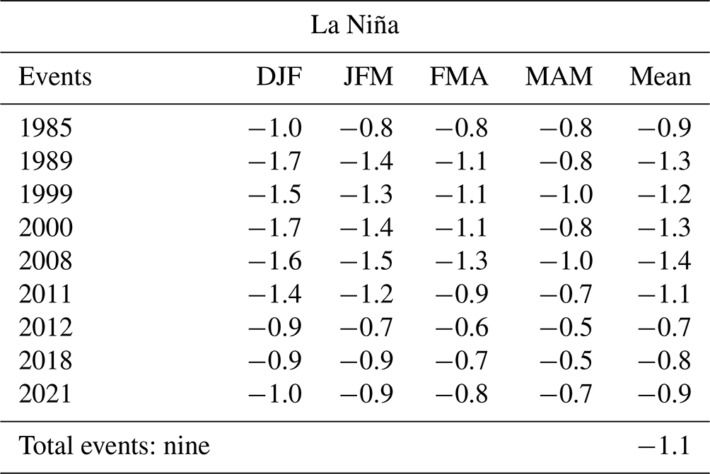
In view of the fact that the relationship between the positive and negative ENSO phases may not be linear (An and Jin, 2004), we consider El Niño and La Niña events separately. For this purpose, we perform composite analyses of ozone, SST, geopotential height, tropopause height and air temperature during El Niño and La Niña events to further investigate the linkage between ENSO and TP TCO. The composite is calculated by the average of the variable during persistent ENSO events. The statistical significance of the composite is tested by the two-tailed Student t test (i.e. Kiladis and Diaz, 1989; von Storch and Zwiers, 1999). The persistent ENSO events are based on the definition of NOAA Climate Prediction Center and our lead–lagged correlation results. We identify persistent El Niño (La Niña) events if their anomalous Niño 3.4 index is greater (less) than 0.5 K (−0.5 K) from winter (December–January–February; DJF) to spring (March–April–May; MAM). There are seven and nine events of persistent El Niño and La Niña (Tables 1–2), respectively.
Table 1List of persistent El Niño events and their anomalous Niño 3.4 index (K) over the period 1979–2021. The final row is the number of total events, and the last column is the corresponding mean of Niño 3.4 index for total events. The DJF, JFM, FMA and MAM indicate December–January–February, January–February–March, February–March–April and March–April–May, respectively.
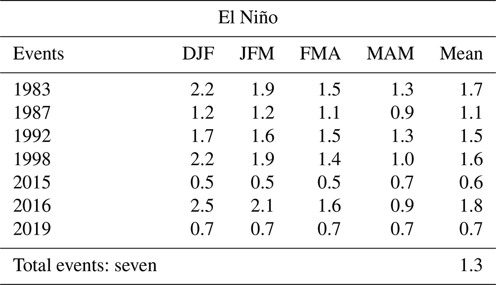
Table 2Same as Table 1 but for La Niña events. The anomalous Niño 3.4 index (K) of these events is less than −0.5 K.
For the tropopause height, we follow the same definition based on the World Meteorological Organization (WMO, 1957), which is identified by the temperature lapse rate. Following the hypsometric equation, the mean temperature of the atmospheric layer between the pressure p1 and p2 can be written as follows (Wallace et al., 1996; Holton and Hakim, 2013; Sun et al., 2017; Li et al., 2022):
where 〈T〉 is the mean temperature of the atmospheric layer; ΔZ is the thickness of the layer; Z1 and Z2 are, respectively, the geopotential heights at p1 and p2; g0=9.80665 m s−2 is the global average of gravity at mean sea level; and R=287 J kg−1 K−1 is the gas constant for dry air. If we let 〈T〉′ and ΔZ′ be the deviations or anomalies from their time average, then Eq. (2) changes to the perturbation hypsometric equation as follows:
The above equation (Eq. 3) suggests that the anomalous mean temperature of the layer is proportional to the anomalous thickness of the layer bounded by isobaric surfaces. Therefore, the mean temperature should decrease (increase) if the perturbed layer thins (thickens). Following previous studies (e.g. Wallace et al., 1996; Sun et al., 2017; Li et al., 2022; Zhang et al., 2022), we use this perturbation equation (Eq. 3) to discuss the influences of atmospheric thickness on tropospheric temperature.
In this section, we first examine whether the TOMCAT can reproduce the TCO variability over the TP by the comparison with the observed satellite TCO from C3S dataset. Figure 1 shows the correlation coefficients between the time series of 3-month running averaged TCO anomalies over the TP (27.5–37.5° N, 75.5–105.5° E) for the C3S dataset and TOMCAT over the period 1979–2021. This averaged TP region is identical to Li et al. (2020). All correlation coefficients between the C3S dataset and TOMCAT in Fig. 1 are high (above 0.65) and are statistically significant at the 99 % level based on the two-tailed Student t test and the Neff of degrees of freedom defined in Eq. (1). In particular, from winter (DJF) to spring (MAM), the correlation coefficients are higher (above 0.95, Fig. 1), indicating that the TP TCO variability of TOMCAT is consistent with that of C3S dataset. It is also noted that the correlation coefficient of monthly time series of TP TCO between C3S dataset and TOMCAT is about 0.92 and is statistically significant at the 99 % level. These results indicate that TOMCAT reproduces the observed TCO variability over the TP well, especially from winter to spring.
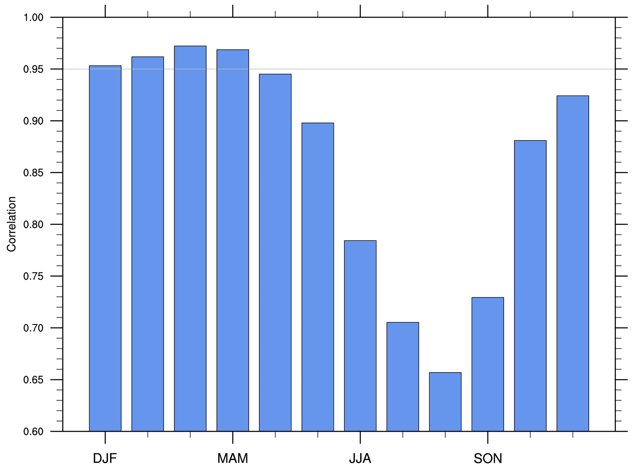
Figure 1Correlation coefficients between the time series of 3-month running mean TCO anomalies over the TP region (27.5–37.5° N, 75.5–105.5° E) for the C3S dataset and the TOMCAT simulation during 1979–2021. All correlation coefficients are statistically significant at 99 % confidence level. The grey line represents the correlation coefficient equal to 0.95.
3.1 Impacts of ENSO on the TCO and ozone profile
ENSO events peak in winter (DJF) and then decay in the following spring (MAM) and summer (JJA). To investigate the linkage between ENSO and TP TCO, we now investigate the lead–lagged correlation coefficients between the TCO (C3S dataset – blue line; TOMCAT result – red line) and the winter (peak season, DJF-averaged) Niño 3.4 index (Fig. 2a). Both the C3S dataset and TOMCAT results show that the significant ENSO signal appears in the TCO before the ENSO's decay in MAM and the strongest ENSO signal appears in the late winter–early spring (Fig. 2a). It is observed that the standard deviation (SD) in both the C3S dataset and TOMCAT results is greater pre-MAM than post-MAM (bars in Fig. 2a) in spite of the model's overestimation, indicating that ENSO may make a greater contribution to the TCO variability from DJF to MAM. Although the TOMCAT overestimates the SD (Fig. 2a) because of its biases (Li et al., 2022), it can be seen from Fig. 2a that TOMCAT matches the SD variability and correlation coefficients well with ENSO in the C3S dataset. These biases of TOMCAT simulation are likely due to (1) the incomplete representation of complex atmospheric process in the TOMCAT or (2) the uncertainties in the TOMCAT's meteorology (ERA5 reanalysis) (Mitchell et al., 2020; Dhomse et al., 2021). Nevertheless, the high correlation (above 0.95, Fig. 1) of TP TCO between the C3S dataset and the TOMCAT simulation from DJF to MAM gives us confidence that the TOMCAT is able to capture the observed variability in TP TCO during these seasons and that we can thus use it to investigate the impact of ENSO on the TP TCO change. Overall, these results suggest that the significant response of TCO over the TP to ENSO may extend from winter of ENSO's mature phase to the spring of the decaying phase.
Some studies suggested there is a link between QBO and ENSO (Baldwin et al., 2001; Anstey et al., 2022), and the QBO is another potential important source of interannual variability of TCO above the TP. To clarify the robust linkage between ENSO and TP TCO, we first remove the QBO signal from TP TCO and then perform lead–lagged correlation, shown in Fig. 2b. The QBO index at 30 and 10 hPa (QBO30 and QBO10) is usually used as the QBO signal (e.g. Baldwin et al., 2001; Li et al., 2020). The TCO associated with QBO (TCOQBO) and TCO after linearly removing QBO signal (TCOremoveQBO) (e.g. Randel et al., 2009) can be written as follows:
where t is corresponding to months; C is a constant; and a and b are the time-dependent regression coefficients of QBO30 and QBO10, respectively.
Figure 2b shows lead correlation coefficients between the ENSO index and the TP TCO without the QBO signal. Lead correlation both with and without the QBO signal is significant from DJF to MAM (Fig. 2). Meanwhile, the lead correlation without the QBO signal (Fig. 2b) is stronger than raw correlation (Fig. 2a), which may be related to excluding the interference of the QBO signal. Our results indicate that the linkage between ENSO and the TP TCO is robust with or without the QBO signal. Therefore, the following composite TCO anomalies are averaged from DJF to MAM to maximise the signal, while we should note the general relationship between ENSO and TCO is not sensitive to the chosen period as one could expect from the positive correlation from DJF to MAM.
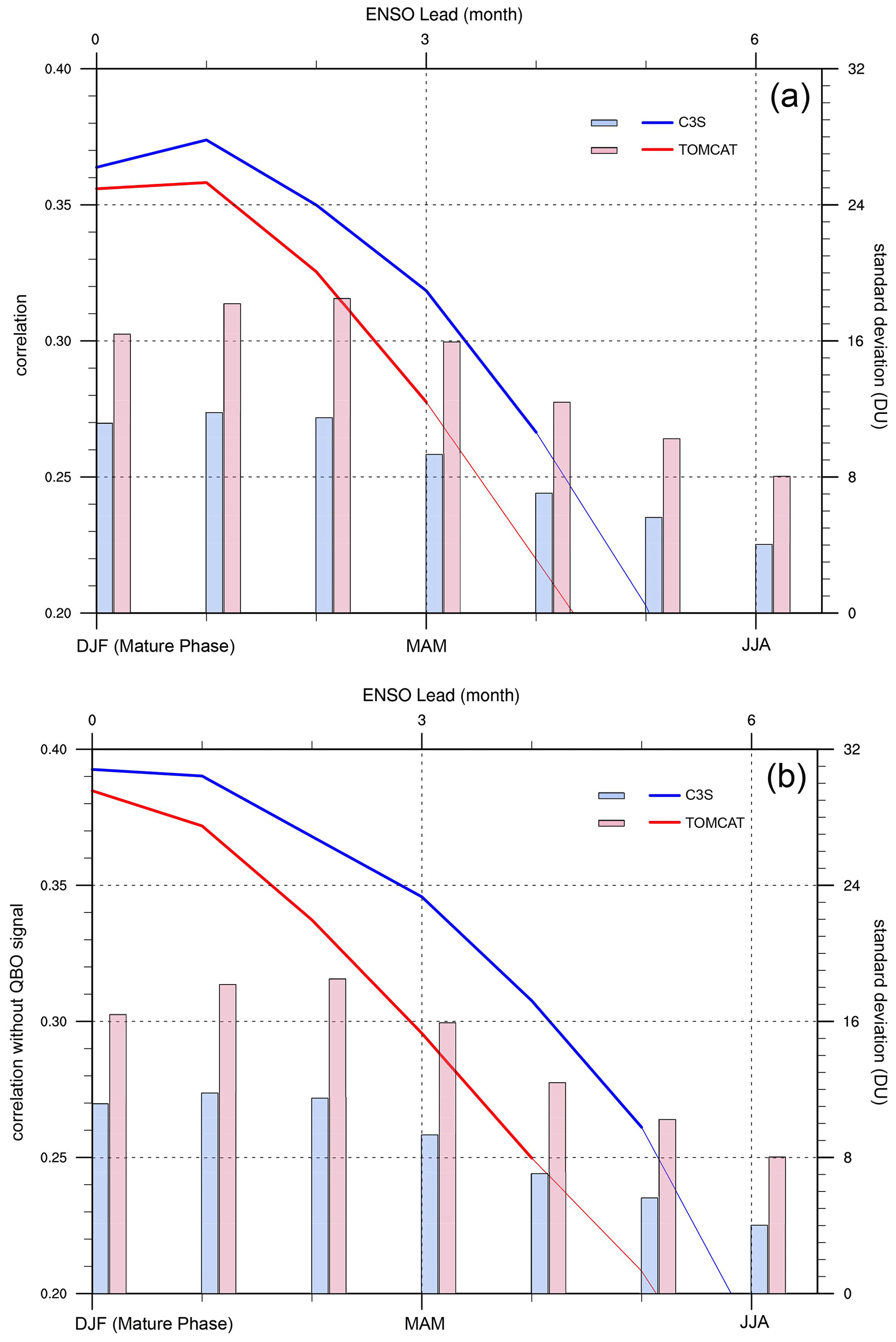
Figure 2(a) Lead-lagged correlation between the time series of averaged TCO anomalies over the TP region (27.5–37.5° N, 75.5–105.5° E) and winter (DJF) Niño 3.4 index for the period 1979–2021. Blue (red) line indicates C3S dataset (TOMCAT result). In the top X axis, positive leads indicate that ENSO is leading. Lead values of 0, 3 and 6 indicate DJF, MAM and JJA, respectively. Thicker lines indicate statistical significance at the 99 % confidence level. Bars (C3S – blue; TOMCAT – red) are standard deviations (DU) of TCO to measure its variability. (b) Same as (a) but without considering the QBO signal on the TP TCO.
Figure 3 shows composite anomalies of the TCO associated with the El Niño and La Niña events in Tables 1–2. The TCO spatial patterns between El Niño and La Niña events are generally opposite despite some differences (Fig. 3), which may be related to the asymmetric features in ENSO itself and its climate impacts (Hoerling et al., 1997; An and Jin 2004; Gao et al., 2019). Although the spatial pattern and also the values of anomalies of C3S and TOMCAT are consistently different (Fig. 3) due to the model's biases (Dhomse et al., 2021), the El Niño (La Niña) events correspond to the significantly positive (negative) TCO anomalies over the whole TP in both the C3S dataset and TOMCAT results (Fig. 3). This result is consistent with that of correlation coefficients (Fig. 2), highlighting the potential influence of ENSO on TCO over the TP. On average, the ENSO events correspond to about ±3.5 DU of the TP TCO anomaly as evaluated in the C3S dataset. As the response of TCO over the TP to ENSO is consistent from DJF to MAM (Fig. 2), it is worth noting that the composite results of TCO are not sensitive to the length of composite seasons from DJF to MAM. On the whole, both the C3S measurement-based dataset and TOMCAT model results show that ENSO has a potential effect on the TCO over the TP. To be specific, it is likely a prolonged impact from DJF of the ENSO's mature phase until MAM of the decaying phase, and the El Niño (La Niña) events favour the positive (negative) TCO anomalies. To better understand the effect of ENSO on the TCO, it is necessary to investigate the vertical ozone changes associated with ENSO.
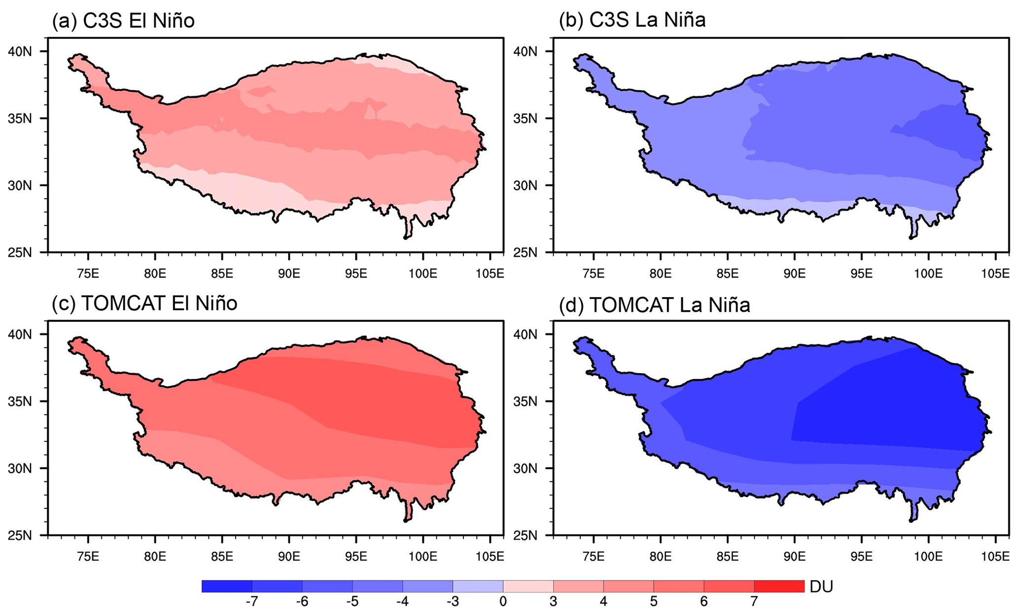
Figure 3Composite anomalies of the TCO (DU) for (a, c) El Niño and (b, d) La Niña events from DJF of ENSO's mature phase to MAM of the decaying phase. Panels (a)–(b) are derived from the C3S dataset, and panels (c)–(d) are derived from TOMCAT results. Coloured regions indicate statistical significance at the 90 % confidence level, and the black line represents the boundary of the TP.
Figure 4 shows composite percentage change (i.e. anomaly divided by climate mean) of the ozone profiles for the El Niño and La Niña events. To make a direct and convenient comparison, here we interpolate the TOMCAT model level (sigma-pressure coordinate) results to the same SWOOSH vertical resolution (pure pressure level). From the SWOOSH dataset and TOMCAT results, Fig. 4 depicts that the El Niño (La Niña) events correspond to the remarkable increase (decrease) of ozone percentage change (about ±6 %) at 200–70 hPa, which is in the upper troposphere and lower stratosphere (UTLS) region. Such ozone increase (decrease) in the profile (Fig. 4) is in good agreement with the downward (upward) shift of ozone profile compared to the climate mean (Fig. 5a and d). To further amplify the differences between the composite ozone profiles and climate mean, we zoom in on the ozone profile at 200–100 hPa (Fig. 5b and e) and 100–50 hPa (Fig. 5c and f). These changes in ozone profiles further contribute to the positive (negative) TCO anomalies over the TP during the El Niño (La Niña) events. Although there are disagreements between the TOMCAT and SWOOSH dataset due to the model's biases (Dhomse et al., 2021), the ENSO events correspond to the significantly ozone change at 200–70 hPa in both the TOMCAT simulation and the SWOOSH dataset.
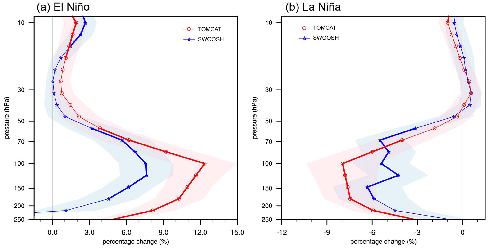
Figure 4Composite percentage change (%) of the ozone profiles with standard deviation (shaded areas) for (a) El Niño and (b) La Niña over the TP region (27.5–37.5° N, 75.5–105.5° E) from DJF in ENSO's mature phase to MAM in the decaying phase. Red lines are derived from TOMCAT, and blue lines are derived from the SWOOSH dataset; thick lines indicate values which exceed the 90 % confidence level.
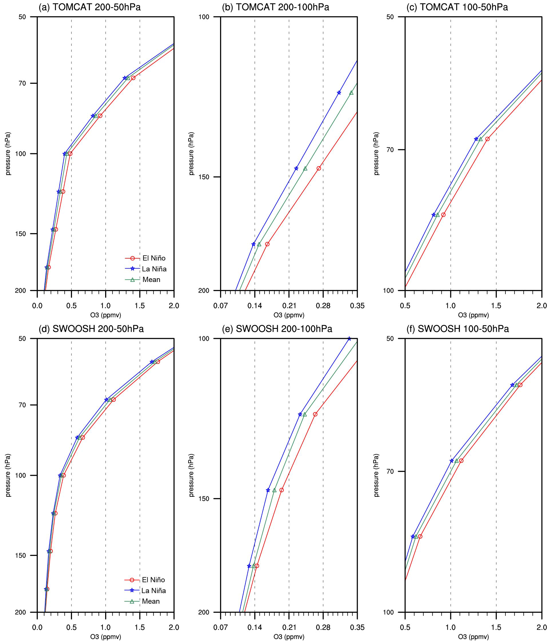
Figure 5Composites and climate means of the ozone profiles from (a) the TOMCAT result and (d) SWOOSH dataset over the TP region (27.5–37.5° N, 75.5–105.5° E) from DJF of ENSO's mature phase to MAM of the decaying phase. Panels (b)–(c) are as in (a) but for a zoomed-in view of the 200–100 and 100–50 hPa domains of (a), respectively. Panels (e)–(f) are as in (b)–(c) but for the TOMCAT result. Green lines indicate climate means of ozone profiles, red lines indicate composite ozone profiles of El Niño events and blue lines indicate composite ozone profiles of La Niña events.
3.2 Potential mechanism for the impact of ENSO on the TCO
Approximately 90 % of ozone in the atmospheric column resides in the stratosphere; the ozone concentration is much lower in the troposphere, with a gradual transition at the tropopause height (TH). Therefore, the increasing (decreasing) TH will tend to carry ozone-poor (ozone-rich) tropospheric (stratospheric) air into the UTLS region and thus decrease (increase) the partial column ozone, which in turn contributes to the TCO decrease (increase) (e.g. Schubert and Munteanu, 1988; Salby and Callaghan, 1993; Steinbrecht et al., 1998; Chipperfield et al., 2003; Varotsos et al., 2004; Tian et al., 2007). Figure 6a–b show composite anomalies of the tropopause pressure for the El Niño and La Niña events. The El Niño (La Niña) events generally correspond to positive (negative) tropopause pressure anomalies over almost the whole TP, where the significant anomalies are located broadly between 30 to 35° N (Fig. 6a–b). These results indicate that the El Niño (La Niña) events may induce a sinking (lifting) TH above the TP. Considering that the area-averaged climate mean of the TH over the whole TP is about 150 hPa from winter to spring, Fig. 6c–d show the composite anomalies of the partial column ozone at 150 hPa. Their spatial patterns (Fig. 6c–d) are in good agreement with the composite TH anomalies (Fig. 6a–b), highlighting the good coherence between the ozone changes and the tropopause changes.
Figure 6e–f show the latitude–height section averaged in longitude (from 75.5 to 105.5° E) of the composite partial column ozone anomalies and tropopause height. During the El Niño events (Fig. 6e), the sinking TH (green line) compared to its climate mean (purple line) corresponds to the significantly positive anomalies of partial column ozone at about 200–70 hPa, which is consistent with the composite percentage change of the ozone profile associated with El Niño events in Fig. 4a. Such positive partial column ozone anomalies related to El Niño events further contribute to the positive TCO anomalies (Fig. 3a and c). The La Niña events correspond to the opposite sign in comparison to the El Niño events (Fig. 6). Specifically, the lifting TH (green line in Fig. 6f) relative to its mean (purple line) favours the negative partial column ozone anomalies, further contributing to the negative TCO anomalies during the La Niña events (Fig. 3b and d).
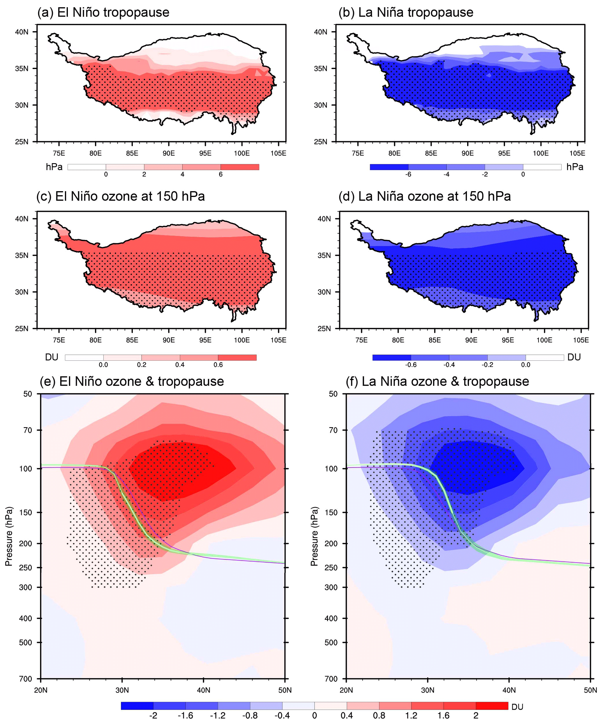
Figure 6Composite anomalies of tropopause pressure (hPa) for (a) El Niño and (b) La Niña events from ERA5 dataset over the TP. Panels (c)–(d) are as in panels (a)–(b) but for partial column ozone anomalies (DU) at 150 hPa. Latitude–height section of the composite partial column ozone anomalies (DU, averaged from 75.5 to 105.5° E) for (e) El Niño and (f) La Niña from TOMCAT. All variables are averaged from DJF of ENSO's mature phase to MAM of the decaying phase. Stippled regions indicate statistical significance at the 90 % confidence level. Purple lines in (e)–(f) indicate the climate mean of tropopause; green lines with standard deviation (shaded areas) indicate the composite tropopause for (e) El Niño and (f) La Niña, respectively; and thick green lines indicate the composite tropopause which exceed the 90 % confidence level.
According to Eq. (3), the anomalous tropospheric upper-level geopotential height can induce the tropospheric temperature change via modifying the air thickness (e.g. Wallace et al., 1996; Sun et al., 2017; Li et al., 2022). As the TH is closely related to tropospheric temperature change (e.g. Seidel and Randel, 2006), it is suggested that the anomalous upper-level geopotential height could influence the TH change. Given that the SSTA associated with ENSO plays a vital role in geopotential height anomalies (e.g. Trenberth et al., 1998), Fig. 7a–b show composites of SSTAs from DJF of ENSO's mature phase to MAM of the decaying phase. The maximum SSTA can clearly be seen in the central and eastern tropical Pacific for the El Niño and La Niña events. Aside from the signal over the tropical Pacific, there is also a significant signal over the tropical Indian Ocean, where the El Niño (La Niña) events correspond to a basin-wide warming (cooling) SSTA. Previous studies have demonstrated that the basin-wide warming (cooling) over the tropical Indian Ocean is a response to surface heat flux changes induced by El Niño (La Niña) (e.g. Alexander et al., 2002; Lau and Nath, 2003; Yang et al., 2007; Schott et al., 2009).
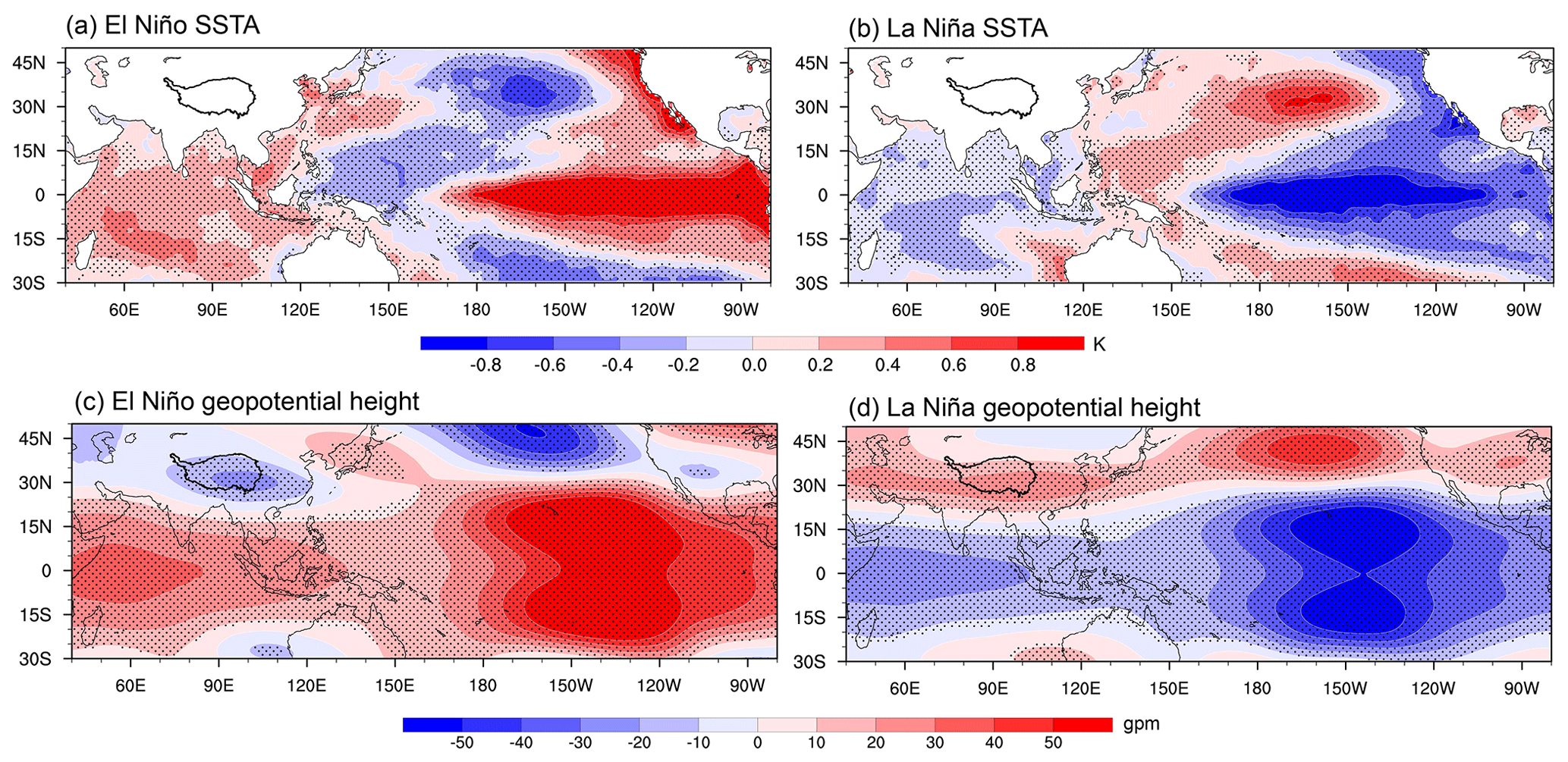
Figure 7Composites of SSTA (K) for (a) El Niño and (b) La Niña from the HadISST1 dataset from DJF of ENSO's mature phase to MAM of the decaying phase. Panels (c)–(d) are as in (a)–(b) but for geopotential height (gpm) anomalies at 150 hPa from the ERA5 dataset. Stippled regions indicate statistical significance at the 90 % confidence level. The black lines represent the boundary of the TP.
Figure 7c–d display the composites of upper-level geopotential height at 150 hPa (GH150) for the ENSO events derived from ERA5 dataset from DJF of ENSO's mature phase to MAM of the decaying phase. The spatial pattern of GH150 over the tropical Pacific and Indian Ocean is in agreement with previous studies focused on atmospheric response to ENSO (e.g. Matsuno, 1966; Gill, 1980; Wallace and Gutzler, 1981; Jin and Hoskins, 1995; Xie et al., 2016). The possible mechanism for the ENSO teleconnection over the TP has been discussed by previous studies, including excited Rossby waves from the tropical Pacific and Indian Ocean to extratropical regions (e.g. Jin and Hoskins, 1995; Trenberth et al., 1998; Zhang et al., 2015b) and enhanced land–sea temperature contrast between the tropical Indian Ocean and the TP (e.g. Chen and You, 2017; Zhao et al., 2018). The latter has been supported by our findings showing a cold 2 m surface air temperature anomaly over the TP during El Niño and vice versa for La Niña (not shown). These results highlight the important role of ENSO in the upper-level geopotential height over the TP. That is, the El Niño (La Niña) events favour negative (positive) GH150 anomalies (Fig. 7).
Based on Eqs. (2)–(3), such anomalous GH150 associated with ENSO can induce air thickness anomalies and thereby influence the tropospheric air temperature. Over the TP, we calculated the monthly time series of tropospheric mean temperature and temperature associated with air thickness that is estimated via the layer from 700 to 150 hPa thickness according to Eq. (3). Basically, their values are about the same (Fig. 8), and their correlation coefficient is close to 1.0, indicating that tropospheric mean temperature is closely related to the air thickness. That is, the increased (decreased) air column thickness associated with the rising (falling) GH150 favours the warming (cooling) tropospheric temperature. Although the TH can be influenced by both stratospheric and tropospheric processes, here we show that the TH over the TP associated with ENSO is dominated by the tropospheric air thickness. We will address this finding by tracing the ENSO signal to the tropospheric air thickness and associated tropospheric temperature. Figure 8a–b show maps of the composites of temperature associated with air thickness. Significantly negative temperature anomalies associated with thickness occur during the El Niño events (Fig. 8a) and vice versa for La Niña (Fig. 8b). It is not surprising that these composite pattern and magnitudes (Figs. 8a–b and S2) are generally the same as those of tropospheric mean temperature (Figs. 8c–8d and S2) because of their close relationship. According to Eq. (3), this implies that the El Niño (La Niña) events favour the decreased (increased) air thickness and thus are associated with the cooling (warming) tropospheric mean temperature (Fig. 8).
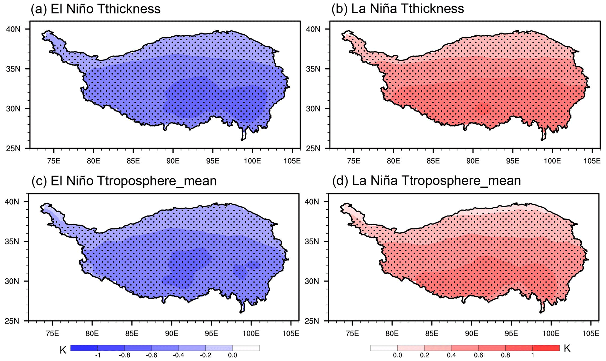
Figure 8Composite anomalies of the temperature (K) anomalies estimated via the layer (700–150 hPa) thickness (Tthickness) for (a) El Niño and (b) La Niña events derived from the ERA5 dataset from DJF of ENSO's mature phase to MAM of the decaying phase. Panels (c)–(d) are as in (a)–(b) but for the tropospheric mean temperature (K) anomalies (Ttroposphere_mean). Note that we calculate the tropospheric mean temperature from 700 to 150 hPa because of the altitude of the TP (about 700 hPa) and the mean TH (about 150 hPa). Stippled regions indicate statistical significance at the 90 % confidence level. The black lines represent the boundary of the TP.
To further show the relationship between ENSO and the tropospheric air thickness and temperature, in Fig. 9a we plotted the temperature associated with air thickness (calculated from Eq. 3) as a function of the ENSO index (Niño 3.4). From the scatter diagram, it is shown that there is a strong negative correlation (−0.56) between Niño 3.4 and temperature associated with air thickness. The relationship is significant (p<0.01 or above the 99 % confidence level), meaning the changes of ozone during the majority of ENSO events are coherent with the composite anomalies (Fig. 8). Another ENSO index (Niño 3; area-averaged SSTA in 5° S–5° N, 90–150° W) has about the same correlation as the Niño 3.4 index. Meanwhile, the correlation coefficient between non-ENSO events (Niño 3.4 index is less than 0.5 K and greater than −0.5 K) and their corresponding temperature associated with air thickness is about −0.12 (p>0.1), suggesting that there is no relationship between them. These results further indicate that the cooling (warming) temperature associated with air thickness is closely related to the El Niño (La Niña) events (Fig. 9a). In addition, Fig. 9b shows the tropopause pressure as a function of the temperature associated with air thickness for ENSO events. The significantly strong negative correlation (−0.85, p<0.01) between them implies that TH over the TP associated with ENSO is dominated by the tropospheric air thickness. The good separation between El Niño and La Niña groups is also coherent with composite results, with most El Niño (La Niña) events corresponding to a cooler (warmer) tropospheric temperature and a lower (higher) TH. In summary, these results suggest that the El Niño (La Niña) events can modulate upper-level geopotential height (Fig. 7), induce thinning (thickening) atmospheric thickness over the TP (Figs. 8 and 9a), contribute to the cooling (warming) tropospheric temperature (Figs. 8 and 9a) and finally favour the sinking (lifting) of the TH (Fig. 9b).
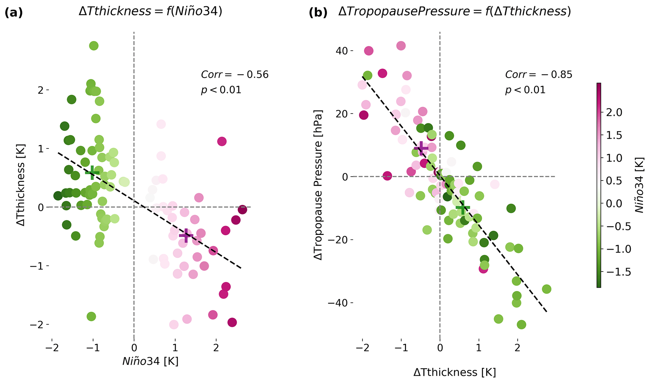
Figure 9(a) The temperature associated with air thickness (Tthickness, unit: K, calculated from Eq. 3) as a function of Niño 3.4 (K) for El Niño (purple circles) and La Niña (green circles) events. (b) The tropopause pressure (hPa) as a function of Tthickness for El Niño (purple circles) and La Niña (green circles) events. The averaged values for El Niño and La Niña events are shown as pluses, and the linear regression lines are shown as dashed black lines. The colour bar shows the intensity of El Niño and La Niña events.
This study aims to investigate the influence of ENSO on the total column ozone (TCO) over the Tibetan Plateau (TP) and its associated potential dynamical mechanism using merged satellite measurements, TOMCAT model output, ERA5 reanalysis and HadISST1 datasets. Our results show that the correlation coefficient between the monthly TP's TCO time series of TOMCAT results and the merged satellite TCO from C3S dataset is high (about 0.92) over the period 1979–2021 and that the correlation coefficient is statistically significant at the 99 % level based on the two-tailed Student t test and the Neff of degrees of freedom. In particular, for DJF, JFM, FMA and MAM, the TOMCAT results and C3S data are highly correlated (above 0.95, Fig. 1), indicating that the TCO variability over the TP in the TOMCAT and C3S dataset is very similar from winter (DJF) to spring (MAM). Therefore, we use these data to investigate the impact of ENSO on the TCO over the TP.
Through analysis of the lead–lagged correlation between ENSO and TP TCO and the composite of TP TCO with and without the QBO signal, both C3S dataset and TOMCAT results show that the significant response of TCO to ENSO is from DJF in its mature phase to MAM in its decaying phase (Fig. 2). In its positive-phase (El Niño) events from DJF to MAM, it corresponds to positive TCO anomalies over the TP, with conditions reversed for the negative-phase (La Niña) events (Fig. 3). The TCO variability associated with the El Niño and La Niña events is closely related to the ozone profile change. The SWOOSH dataset and TOMCAT results show that the El Niño (La Niña) events mainly modulate the level of ozone centred at 200–70 hPa (Fig. 4) and therefore favour the positive (negative) TCO anomalies (Fig. 3).
We highlight the potential mechanism for the impact of ENSO on the TCO over the TP from DJF to MAM. Our results suggest that El Niño can trigger the TP TCO change via the following potential processes. Firstly, the El Niño events tend to exert the negative upper-level geopotential height anomaly (Fig. 7) via the El Niño teleconnection and land–sea temperature contrast associated with El Niño, thus corresponding to the decreasing air thickness (Fig. 8a–b) based on Eq. (2) and previous studies (e.g. Wallace et al., 1996; Sun et al., 2017). Secondly, according to Eq. (3), the thickness decrease could reduce the tropospheric temperature over the TP (Fig. 8c–d), which further induces a decrease in the TH (Fig. 6) in terms of the tropopause definition of WMO (1957) and our results (Fig. 9). Thirdly, such a TH decrease tends to induce a change in the relative amounts of ozone-poor tropospheric and ozone-rich stratospheric air in the profile, which increases the partial column ozone in the UTLS (Figs. 4 and 6) and thus contributes to the TCO increase (Fig. 3). The linkage between La Niña events and TP TCO as well as its associated processes resembles the El Niño events, except with anomalies of opposite sign. Our results suggest the El Niño (La Niña) events play an important role in the TCO variability over the TP, which has implications for a better understanding of factors controlling the interannual variability of ozone.
To further verify our statistical results, we designed and performed a series of model experiments to isolate the influence of ENSO. Since many studies have used the NCAR Community Atmosphere Model version 4 (CAM4) to isolate the SST-forced responses (e.g. Neale et al., 2013; Warner et al., 2020; Pausata et al., 2023), we use CAM4 to support our findings. CAM4 is the atmospheric component of the Community Earth System Model (CESM) and has a horizontal resolution of 1.9° (latitude) ×2.5° (longitude) and 26 vertical levels. Three experiments are described in Table S1 in the Supplement, all of which are the same except for different SST forcings. The experiments were each run for 30 years, with the first 5 years excluded as a spin-up period. The remaining 25 years was used for the analysis. As the tropopause height (TH) variability plays a key role in our potential mechanism, in Fig. S3 we display the TH responses to El Niño and La Niña, averaged from December to May, when the response is significant (Fig. 2). Figure S3 shows that El Niño (La Niña) generally corresponds to a positive (negative) tropopause pressure difference over almost the whole TP, which is in good agreement with the composite pattern associated with El Niño (La Niña) events (Fig. 6a–b). Note that the simulated intensity of tropopause pressure is stronger than that of the composite in observations, which may be due to deficiencies in the model parameterisation scheme over the TP. Nevertheless, these simulations do support our statistical results.
In this study, we have provided a systematic explanation of the impacts of ENSO on the TCO over the TP via the TH. Although Fig. 9 is in good agreement with our study and shows that there are significant correlations between samples of ENSO events and air thickness as well as the TH, it is also apparent that a few samples deviate from the regression line and have limited change. This implies that in addition to ENSO, there may be other factors contributing to the air thickness and TH variability and thus contributing to the TCO variation. Recently, Duan et al. (2023) stated that the tropical Indian Ocean SSTA could cause a vertical shift of the ozone profile over the TP and thus contribute to the TCO variation. Their study differs from ours, as we focus on ENSO with the strongest interannual SSTA. Considering the close relationship between ENSO and tropical Indian and Atlantic Oceans, it will be interesting to study their individual and combined effects on the TP's TCO. Our study focuses on the diagnosed ozone changes over the TP during ENSO episodes using both observations and a chemistry transport model TOMCAT as well as several statistical methods, which will have some uncertainties due to large internal variability of ozone and limited ENSO events. Future work is needed for a better understanding of ENSO impacts with more observed ENSO events and a fully coupled chemistry–climate model.
The code used to generate the figures in this paper is available from the corresponding authors upon request.
The C3S satellite product is available from https://doi.org/10.24381/cds.4ebfe4eb (Copernicus Climate Change Service, 2020). The SWOOSH data are available from https://csl.noaa.gov/groups/csl8/swoosh/ (Davis et al., 2016). The ERA5 product can be found at https://doi.org/10.24381/cds.6860a573 (Hersbach et al., 2023). The HadISST1 data are available from https://www.metoffice.gov.uk/hadobs/hadisst/ (Rayner et al., 2003). The Niño 3.4 index can be found at https://psl.noaa.gov/gcos_wgsp/Timeseries/Nino34/ (NOAA-PSL, 2023). The QBO index is available at https://www.geo.fu-berlin.de/en/met/ag/strat/produkte/qbo/index.html (Baldwin et al., 2001). The El Niño and La Niña events by seasons can be found at https://origin.cpc.ncep.noaa.gov/products/analysis_monitoring/ensostuff/ONI_v5.php (NOAA-CPC, 2024). The TP boundary dataset is available from https://www.geodoi.ac.cn/edoi.aspx?DOI=10.3974/geodb.2014.01.12.V1 (Zhang et al., 2002). The model output used for the figures is available from https://doi.org/10.5281/zenodo.8383878 (Li et al., 2023).
The supplement related to this article is available online at: https://doi.org/10.5194/acp-24-8277-2024-supplement.
YL performed the data analysis and prepared the manuscript. WF, MPC, XZ and YL gave support with discussion, simulation and interpretation and helped to write the paper.
The contact author has declared that none of the authors has any competing interests.
Publisher’s note: Copernicus Publications remains neutral with regard to jurisdictional claims made in the text, published maps, institutional affiliations, or any other geographical representation in this paper. While Copernicus Publications makes every effort to include appropriate place names, the final responsibility lies with the authors.
The authors thank the Copernicus Climate Change Service (C3S), ECMWF, NOAA and Met Office Hadley Centre for providing data. The modelling work is supported by the University of Leeds and National Centre for Atmospheric Science (NCAS). This work was jointly supported by the National Natural Science Foundation of China (grant nos. 42175042, 42275059 and U20A2097), the Natural Science Foundation of Sichuan Province (grant nos. 2024NSFTD0017 and 2023NSFSC0246), the China Scholarship Council (grant nos. 201908510031 and 201908510032) and the Jiangsu Province Natural Science Foundation Youth Fund Project (grant no. BK20230115). The TOMCAT modelling work was also supported by the UK Natural Environment Research Council (NERC; grant no. NE/V011863/1).
This research has been supported by the National Natural Science Foundation of China (grant nos. 42175042, 42275059 and U20A2097), the Natural Science Foundation of Sichuan Province (grant nos. 2024NSFTD0017 and 2023NSFSC0246) and the UK Natural Environment Research Council (grant no. NE/V011863/1). Wuhu Feng is supported by the NCAS National Capability Single Centre Science Programme (grant no. NE/R015244/1).
This paper was edited by Rolf Müller and reviewed by three anonymous referees.
An, S. I. and Jin, F. F.: Nonlinearity and Asymmetry of ENSO, J. Climate, 17, 2399–2412, https://doi.org/10.1175/1520-0442(2004)017<2399:NAAOE>2.0.CO;2, 2004.
Ahrens, C. D. and Samson, P. J.: Extreme Weather and Climate, 1st Edn. Brooks Cole, 508 pp., https://search-library.ucsd.edu/permalink/01UCS_SDI/desb83/alma991006957539706535 (last access: July 2024), 2011.
Alexander, M. A., Bladé, I., Newman, M., Lanzante, J. R., Lau, N. C., and Scott, J. D.: The atmospheric bridge: the influence of ENSO teleconnections on air–sea interaction over the global oceans, J. Climate, 15, 2205–2231, https://doi.org/10.1175/1520-0442(2002)015<2205:TABTIO>2.0.CO;2, 2002.
Anstey, J. A., Osprey, S. M., Alexander, J., Baldwin, M. P., Butchart, N., Gray, L., Kawatani, Y., Newman, P. A., and Richter, J. H.: Impacts, processes and projections of the quasi-biennial oscillation, Nat. Rev. Earth Environ., 3, 588–603, https://doi.org/10.1038/s43017-022-00323-7, 2022.
Baldwin, M. P., Gray, L. J., Dunkerton, T. J., Hamilton, K., Haynes, P. H., Randel, W. J., Holton, J. R., Alexander, M. J., Hirota, I., Horinouchi, T., Jones, D. B. A., Kinnersley, J. S., Marquardt, C., Sato, K., and Takahashi, M.: The quasi-biennial oscillation, Rev. Geophys., 39, 179–229, https://doi.org/10.1029/1999RG000073, 2001.
Bian, J., Wang, G., Chen, H., Qi, D., Lü, D., and Zhou, X.: Ozone mini-hole occurring over the Tibetan Plateau in December 2003, Chin. Sci. Bull., 51, 885–888, https://doi.org/10.1007/s11434-006-0885-y, 2006.
Bian, J., Yan, R., Chen, H., Lü, D., and Massie, S. T.: Formation of the summertime ozone valley over the Tibetan Plateau: The Asian summer monsoon and air column variations, Adv. Atmos. Sci., 28, 1318, https://doi.org/10.1007/s00376-011-0174-9, 2011.
Bognar, K., Alwarda, R., Strong, K., Chipperfield, M. P., Dhomse, S. S., Drummond, J. R., Feng, W., Fioletov, V., Goutail, F., Herrera, B., Manney, G. L., McCullough, E. M., Millán, L. F., Pazmino, A., Walker, K. A., Wizenberg, T., and Zhao, X.: Unprecedented spring 2020 ozone depletion in the context of 20 years of measurements at Eureka, Canada, J. Geophys. Res., 126, e2020JD034365, https://doi.org/10.1029/2020JD034365, 2021.
Cai, W., Wang, G., Dewitte, B., Wu, L., Santoso, A., Takahashi, K., Yang, Y., Carréric, A., and McPhaden, M. J.: Increased variability of eastern Pacific El Niño under greenhouse warming, Nature, 564, 201–206, https://doi.org/10.1038/s41586-018-0776-9, 2018.
Cagnazzo, C., Manzini, E., Calvo, N., Douglass, A., Akiyoshi, H., Bekki, S., Chipperfield, M., Dameris, M., Deushi, M., Fischer, A. M., Garny, H., Gettelman, A., Giorgetta, M. A., Plummer, D., Rozanov, E., Shepherd, T. G., Shibata, K., Stenke, A., Struthers, H., and Tian, W.: Northern winter stratospheric temperature and ozone responses to ENSO inferred from an ensemble of Chemistry Climate Models, Atmos. Chem. Phys., 9, 8935–8948, https://doi.org/10.5194/acp-9-8935-2009, 2009.
Carpenter, L. J., Daniel, J. S., Fleming, E. L., Hanaoka, T., Ju, H., Ravishankara, A. R., Ross, M. N., Tilmes, S., Wallington, T. J., and Wuebbles, D. J.: Scenarios and information for policy makers, in: Scientific Assessment of Ozone Depletion: 2018, World Meteorological Organization, Global Ozone Research and Monitoring Project–Report No. 58, Chap. 6, World Meteorological Organization/UNEP, Geneva, Switzerland, https://csl.noaa.gov/assessments/ozone/2018/downloads/Chapter6_2018OzoneAssessment.pdf (last access: July 2024), 2018.
Chang, S., Li, Y., Shi, C., and Guo, D.: Combined effects of the ENSO and the QBO on the ozone valley over the Tibetan Plateau, Remote Sens., 14, 4935, https://doi.org/10.3390/rs14194935, 2022.
Chen, X. and You, Q.: Effect of Indian Ocean SST on Tibetan Plateau precipitation in the early rainy season, J. Climate, 30, 8973–8985, https://doi.org/10.1175/JCLI-D-16-0814.1, 2017.
Chipperfield, M. P., Randel, W. J., Bodeker, G. E., Dameris, M., Fioletov, V. E., Friedl, R. R., Harris, N. R. P., Logan, J. A., McPeters, R. D., Muthama, N. J., Peter, T., Shepherd, T. G., Shine, K. P., Solomon, S., Thomason, L. W., and Zawodny, J. M.: Global Ozone: Past and Present, in: WMO (World Meteorological Organization) Scientific Assessment of Ozone Depletion: 2002, Global Ozone Research and Monitoring Project – Report No. 47, WMO, Geneva, 498 pp., https://csl.noaa.gov/assessments/ozone/2002/chapters/chapter4.pdf (last access: 27 September 2023), 2003.
Chipperfield, M. P.: New version of the TOMCAT/SLIMCAT off-line chemical transport model: Intercomparison of stratospheric tracer experiments, Q. J. Roy. Meteorol. Soc., 132, 1179–1203, https://doi.org/10.1256/qj.05.51, 2006.
Chipperfield, M. P., Bekki, S., Dhomse, S., Harris, N. R. P., Hassler, B., Hossaini, R., Steinbrecht, W., Thiéblemont, R., and Weber, M.: Detecting recovery of the stratospheric ozone layer, Nature, 549, 211–218, https://doi.org/10.1038/nature23681, 2017.
Chipperfield, M. P., Dhomse, S., Hossaini, R., Feng, W., Santee, M. L., Weber, M., Burrows, J. P., Wild, J. D., Loyola, D., and Coldewey-Egbers, M.: On the cause of recent variations in lower stratospheric ozone, Geophys. Res. Lett., 45, 5718–5726, https://doi.org/10.1029/2018GL078071, 2018.
Copernicus Climate Change Service, Climate Data Store: Ozone monthly gridded data from 1970 to present derived from satellite observations, Copernicus Climate Change Service (C3S) Climate Data Store (CDS) [data set], https://doi.org/10.24381/cds.4ebfe4eb, 2020.
Davis, S. M., Rosenlof, K. H., Hassler, B., Hurst, D. F., Read, W. G., Vömel, H., Selkirk, H., Fujiwara, M., and Damadeo, R.: The Stratospheric Water and Ozone Satellite Homogenized (SWOOSH) database: a long-term database for climate studies, Earth Syst. Sci. Data, 8, 461–490, https://doi.org/10.5194/essd-8-461-2016, 2016.
Dhame, S., Taschetto, A. S., Santoso, A., and Meissner, K. J.: Indian Ocean warming modulates global atmospheric circulation trends, Clim. Dynam., 55, 2053–2073, https://doi.org/10.1007/s00382-020-05369-1, 2020.
Dhomse, S. S., Chipperfield, M. P., Feng, W., Ball, W. T., Unruh, Y. C., Haigh, J. D., Krivova, N. A., Solanki, S. K., and Smith, A. K.: Stratospheric O3 changes during 2001–2010: the small role of solar flux variations in a chemical transport model, Atmos. Chem. Phys., 13, 10113–10123, https://doi.org/10.5194/acp-13-10113-2013, 2013.
Dhomse, S. S., Chipperfield, M. P., Feng, W., Hossaini, R., Mann, G. W., and Santee, M. L.: Revisiting the hemispheric asymmetry in midlatitude ozone changes following the Mount Pinatubo eruption: A 3-D model study, Geophys. Res. Lett., 42, 3038–3047, https://doi.org/10.1002/2015GL063052, 2015.
Dhomse, S. S., Chipperfield, M. P., Damadeo, R. P., Zawodny, J. M., Ball, W. T., Feng, W., Hossaini, R., Mann, G. W., and Haigh, J. D.: On the ambiguous nature of the 11-year solar cycle signal in upper stratospheric ozone, Geophys. Res. Lett., 43, 7241–7249, https://doi.org/10.1002/2016GL069958, 2016.
Dhomse, S. S., Arosio, C., Feng, W., Rozanov, A., Weber, M., and Chipperfield, M. P.: ML-TOMCAT: machine-learning-based satellite-corrected global stratospheric ozone profile data set from a chemical transport model, Earth Syst. Sci. Data, 13, 5711–5729, https://doi.org/10.5194/essd-13-5711-2021, 2021.
Domeisen, D. I. V., Garfinkel, C. I., and Butler, A. H.: The teleconnection of El Niño Southern Oscillation to the stratosphere, Rev. Geophys., 57, 5–47, https://doi.org/10.1029/2018RG000596, 2019.
Duan, J., Tian, W., Zhang, J., Hu, Y., Yang, J., Wang, T., and Huang, R.: Impact of the Indian Ocean SST on wintertime total column ozone over the Tibetan Plateau, J. Geophys. Res., 128, e2022JD037850, https://doi.org/10.1029/2022JD037850, 2023.
Feng, W., Chipperfield, M. P., Roscoe, H. K., Remedios, J. J., Waterfall, A. M., Stiller, G. P., Glatthor, N., Höpfner, M., and Wang, D. Y.: Three-dimensional model study of the Antarctic ozone hole in 2002 and comparison with 2000, J. Atmos. Sci., 62, 822–837, https://doi.org/10.1175/JAS-3335.1, 2005.
Feng, W., Chipperfield, M. P., Davies, S., Mann, G. W., Carslaw, K. S., Dhomse, S., Harvey, L., Randall, C., and Santee, M. L.: Modelling the effect of denitrification on polar ozone depletion for Arctic winter 2004/2005, Atmos. Chem. Phys., 11, 6559–6573, https://doi.org/10.5194/acp-11-6559-2011, 2011.
Feng, W., Dhomse, S. S., Arosio, C., Weber, M., Burrows, J. P., Santee, M. L., and Chipperfield, M. P.: Arctic ozone depletion in 2019/20: Roles of chemistry, dynamics and the Montreal Protocol, Geophys. Res. Lett., 48, e2020GL091911, https://doi.org/10.1029/2020GL091911, 2021.
Flohn, H.: Large-scale Aspects of the “summer monsoon” in South and East Asia, J. Meteor. Soc. Japan., 35A, 180–186, https://doi.org/10.2151/jmsj1923.35A.0_180, 1957.
Fusco, A. C. and Salby, M. L.: Interannual variations of total ozone and their relationship to variations of planetary wave activity, J. Climate, 12, 1619–1629, https://doi.org/10.1175/1520-0442(1999)012<1619:IVOTOA>2.0.CO;2, 1999.
Gao, R., Zhang, R., Wen, M., and Li, T.: Interdecadal changes in the asymmetric impacts of ENSO on wintertime rainfall over China and atmospheric circulations over western North Pacific, Clim. Dynam., 52, 7525–7536, https://doi.org/10.1007/s00382-018-4282-4, 2019.
Gill, A.: Some simple solutions for heat-induced tropical circulation, Q. J. Roy. Meteorol. Soc., 106, 447–462, https://doi.org/10.1002/qj.49710644905, 1980.
Griffin, D., Walker, K. A., Wohltmann, I., Dhomse, S. S., Rex, M., Chipperfield, M. P., Feng, W., Manney, G. L., Liu, J., and Tarasick, D.: Stratospheric ozone loss in the Arctic winters between 2005 and 2013 derived with ACE-FTS measurements, Atmos. Chem. Phys., 19, 577–601, https://doi.org/10.5194/acp-19-577-2019, 2019.
Grooß, J.-U., Müller, R., Spang, R., Tritscher, I., Wegner, T., Chipperfield, M. P., Feng, W., Kinnison, D. E., and Madronich, S.: On the discrepancy of HCl processing in the core of the wintertime polar vortices, Atmos. Chem. Phys., 18, 8647–8666, https://doi.org/10.5194/acp-18-8647-2018, 2018.
Guo, D., Wang, P., Zhou, X., Liu, Y., and Li, W.: Dynamic effects of the South Asian high on the ozone valley over the Tibetan Plateau, Acta. Meteor. Sinica., 26, 216–228, https://doi.org/10.1007/s13351-012-0207-2, 2012.
Hasebe, F.: Dynamical Response of the Tropical Total Ozone to Sea Surface Temperature Changes, J. Atmos. Sci., 50, 345–356, https://doi.org/10.1175/1520-0469(1993)050<0345:DROTTT>2.0.CO;2, 1993.
Hersbach, H., Bell, B., Berrisford, P., Hirahara, S., Horányi, A., Muñoz-Sabater, J., Nicolas, J., Peubey, C., Radu, R., Schepers, D., Simmons, A., Soci, C., Abdalla, S., Abellan, X., Balsamo, G., Bechtold, P., Biavati, G., Bidlot, J., Bonavita, M., De Chiara, G., Dahlgren, P., Dee, D., Diamantakis, M., Dragani, R., Flemming, J., Forbes, R., Fuentes, M., Geer, A., Haimberger, L., Healy, S., Hogan, R. J., Hólm, E., Janisková, M., Keeley, S., Laloyaux, P., Lopez, P., Lupu, C., Radnoti, G., de Rosnay, P., Rozum, I., Vamborg, F., Villaume, S., and Thépaut, J.-N.: The ERA5 global reanalysis, Q. J. Roy. Meteorol. Soc., 146, 1999–2049, https://doi.org/10.1002/qj.3803, 2020.
Hersbach, H., Bell, B., Berrisford, P., Biavati, G., Horányi, A., Muñoz Sabater, J., Nicolas, J., Peubey, C., Radu, R., Rozum, I., Schepers, D., Simmons, A., Soci, C., Dee, D., and Thépaut, J.-N.: ERA5 monthly averaged data on pressure levels from 1940 to present, Copernicus Climate Change Service (C3S) Climate Data Store (CDS) [data set], https://doi.org/10.24381/cds.6860a573, 2023.
Hoerling, M. P., Kumar, A., and Zhong, M.: El Niño, La Niña, and the Nonlinearity of Their Teleconnections, J. Climate, 10, 1769–1786, https://doi.org/10.1175/1520-0442(1997)010<1769:ENOLNA>2.0.CO;2, 1997.
Holton, J. R. and Hakim, G. J.: An Introduction to Dynamic Meteorology. 5th Edn., Academic Press, 552 pp., https://doi.org/10.1016/C2009-0-63394-8, 2013.
Jin, F. and Hoskins, B. J.: The direct response to tropical heating in a baroclinic atmosphere, J. Atmos. Sci., 52, 307–319, https://doi.org/10.1175/1520-0469(1995)052<0307:TDRTTH>2.0.CO;2, 1995.
Kiladis, G. N. and Diaz, H. F.: Global climatic anomalies associated with extremes in the Southern Oscillation, J. Climate, 2, 1069–1090, https://doi.org/10.1175/1520-0442(1989)002<1069:GCAAWE>2.0.CO;2, 1989
Kiss, P., Müller, R., and Jánosi, I. M.: Long-range correlations of extrapolar total ozone are determined by the global atmospheric circulation, Nonlin. Processes Geophys., 14, 435–442, https://doi.org/10.5194/npg-14-435-2007, 2007.
Kuttippurath, J., Kleinböhl, A., Bremer, H., Küllmann, H., Notholt, J., Sinnhuber, B.-M., Feng, W., and Chipperfield, M.: Aircraft measurements and model simulations of stratospheric ozone and N2O: implications for chemistry and transport processes in the models, J. Atmos. Chem., 66, 41–64, https://doi.org/10.1007/s10874-011-9191-4, 2010.
Lau, N. C. and Nath, M. J.: Atmosphere–ocean variations in the Indo-Pacific sector during ENSO episodes, J. Climate, 16, 3–20, https://doi.org/10.1175/1520-0442(2003)016<0003:AOVITI>2.0.CO;2, 2003.
Li, J., Sun, C., and Jin, F. F.: NAO implicated as a predictor of Northern Hemisphere mean temperature multidecadal variability, Geophys. Res. Lett., 40, 5497–5502, https://doi.org/10.1002/2013GL057877, 2013.
Li, J., Xie, T., Tang, X., Wang, H., Sun, C., Feng, J., Zheng, F., and Ding, R.: Influence of the NAO on wintertime surface air temperature over East Asia: multidecadal variability and decadal prediction, Adv. Atmos. Sci., 39, 625–642, https://doi.org/10.1007/s00376-021-1075-1, 2022.
Li, Y., Chipperfield, M. P., Feng, W., Dhomse, S. S., Pope, R. J., Li, F., and Guo, D.: Analysis and attribution of total column ozone changes over the Tibetan Plateau during 1979–2017, Atmos. Chem. Phys., 20, 8627–8639, https://doi.org/10.5194/acp-20-8627-2020, 2020.
Li, Y., Dhomse, S. S., Chipperfield, M. P., Feng, W., Chrysanthou, A., Xia, Y., and Guo, D.: Effects of reanalysis forcing fields on ozone trends and age of air from a chemical transport model, Atmos. Chem. Phys., 22, 10635–10656, https://doi.org/10.5194/acp-22-10635-2022, 2022.
Li, Y., Li, J., Zhang, W., Chen, Q., Feng, J., Zheng, F., Wang, W., and Zhou, X.: Impacts of the tropical Pacific cold tongue mode on ENSO diversity under global warming, J. Geophys. Res., 122, 8524–8542, https://doi.org/10.1002/2017JC013052, 2017.
Li, Y., Feng, W., Zhou, X., Li, Y., and Chipperfield, M.: The impact of El Niño–Southern Oscillation on the total column ozone over the Tibetan Plateau, Zenodo [data set], https://doi.org/10.5281/zenodo.8383878, 2023.
Liu, H., Hu, B., Zhang, L., Wang, Y. S., and Tian, P. F.: Spatiotemporal characteristics of ultraviolet radiation in recent 54 years from measurements and reconstructions over the Tibetan Plateau, J. Geophys. Res., 121, 7673–7690, https://doi.org/10.1002/2015JD024378, 2016.
Liu, Y., Li, W., Zhou, X., and He, J.: Mechanism of formation of the ozone valley over the Tibetan Plateau in summer – transport and chemical process of ozone, Adv. Atmos. Sci., 20, 103–109, https://doi.org/10.1007/BF03342054, 2003.
Matsuno, T.: Quasi-geostrophic motions in the equatorial area, J. Meteor. Soc. Japan., 44, 25–43, https://doi.org/10.2151/jmsj1965.44.1_25, 1966.
McPhaden, M. J., Zebiak, S. E., and Glantz, M. H.: ENSO as an integrating concept in earth science, Science, 314, 1740–1745, https://doi.org/10.1126/science.1132588, 2006.
Mitchell, D. M., Eunice Lo, Y. T., Seviour, W. J. M., Haimberger, L., and Polvani, L. M.: The vertical profile of recent tropical temperature trends: Persistent model biases in the context of internal variability, Environ. Res. Lett., 15, 1040b1044, https://doi.org/10.1088/1748-9326/ab9af7, 2020.
Neale, R. B., Richter, J., Park, S., Lauritzen, P. H., Vavrus, S. J., Rasch, P. J., and Zhang, M.: The Mean Climate of the Community Atmosphere Model (CAM4) in Forced SST and Fully Coupled Experiments. J. Climate, 26, 5150–5168, https://doi.org/10.1175/JCLI-D-12-00236.1, 2013.
NOAA-CPC: NOAA Climate Prediction Center, https://origin.cpc.ncep.noaa.gov/products/analysis_monitoring/ensostuff/ONI_v5.php (last access: 22 July 2024), 2024.
Olsen, M. A., Wargan, K., and Pawson, S.: Tropospheric column ozone response to ENSO in GEOS-5 assimilation of OMI and MLS ozone data, Atmos. Chem. Phys., 16, 7091–7103, https://doi.org/10.5194/acp-16-7091-2016, 2016.
Oman, L. D., Ziemke, J. R., Douglass, A. R., Waugh, D. W., Lang, C., Rodriguez, J. M., and Nielsen, J. E.: The response of tropical tropospheric ozone to ENSO, Geophys. Res. Lett., 38, L13706, https://doi.org/10.1029/2011GL047865, 2011.
Pausata, F. S. R., Zhao, Y., Zanchettin, D., Caballero, R., and Battisti, D. S.: Revisiting the mechanisms of ENSO response to tropical volcanic eruptions. Geophys. Res. Lett., 50, e2022GL102183. https://doi.org/10.1029/2022GL102183, 2023.
Pokharel, M., Guang, J., Liu, B., Kang, S., Ma, Y., Holben, B. N., Xia, X., Xin, J., Ram, K., and Rupakheti, D.: Aerosol properties over Tibetan Plateau from a decade of AERONET measurements: baseline, types, and influencing factors, J. Geophys. Res.-Atmos., 124, 13357–13374, https://doi.org/10.1029/2019JD031293, 2019.
Pyper, B. J. and Peterman, R. M.: Comparison of methods to account for autocorrelation in correlation analyses of fish data, Can. J. Fish. Aquat. Sci., 55, 2127–2140, https://doi.org/10.1139/f98-104, 1998.
Randel, W. J., Garcia, R. R., Calvo, N., and Marsh, D.: ENSO influence on zonal mean temperature and ozone in the tropical lower stratosphere, Geophys. Res. Lett., 36, L15822, https://doi.org/10.1029/2009GL039343, 2009.
Rayner, N. A., Parker, D. E., Horton, E. B., Folland, C. K., Alexander, L. V., Rowell, D. P., Kent, E. C., and Kaplan, A.: Global analyses of sea surface temperature, sea ice, and night marine air temperature since the late nineteenth century, J. Geophys. Res., 108, 4407, https://doi.org/10.1029/2002JD002670, 2003.
Ropelewski, C. F. and Halpert, M. S.: Global and regional scale precipitation patterns associated with the El Niño/Southern Oscillation, Mon. Weather Rev., 115, 1606–1626, https://doi.org/10.1175/1520-0493(1987)115<1606:GARSPP>2.0.CO;2, 1987.
Royden, L. H., Burchfiel, B. C., and van der Hilst, R. D.: The geological evolution of the Tibetan Plateau, Science, 321, 1054–1058, https://doi.org/10.1126/science.1155371, 2008.
Rösevall, J. D., Murtagh, D. P., Urban, J., Feng, W., Eriksson, P., and Brohede, S.: A study of ozone depletion in the 2004/2005 Arctic winter based on data from Odin/SMR and Aura/MLS, J. Geophys. Res., 113, D13301, https://doi.org/10.1029/2007JD009560, 2008.
Salby, M. L. and Callaghan, P. F.: Fluctuations of total ozone and their relationship to stratospheric air motions, J. Geophys. Res., 98, 2715–2727, https://doi.org/10.1029/92JD01814, 1993.
Schott, F. A., Xie, S.-P., and McCreary Jr., J. P.: Indian Ocean circulation and climate variability, Rev. Geophys., 47, RG1002, https://doi.org/10.1029/2007RG000245, 2009.
Schubert, S. D. and Munteanu, M. J.: An analysis of tropopause pressure and total ozone correlations, Mon. Weather Rev., 116, 569–582, https://doi.org/10.1175/1520-0493(1988)116<0569:AAOTPA>2.0.CO;2, 1988.
Seidel, D. J. and Randel, W. J.: Variability and trends in the global tropopause estimated from radiosonde data, J. Geophys. Res., 111, D21101, https://doi.org/10.1029/2006JD007363, 2006.
Shiotani, M.: Annual, quasi-biennial, and El Niño-Southern Oscillation (ENSO) time-scale variations in equatorial total ozone, J. Geophys. Res., 97, 7625–7633, https://doi.org/10.1029/92JD00530, 1992.
Singleton, C. S., Randall, C. E., Chipperfield, M. P., Davies, S., Feng, W., Bevilacqua, R. M., Hoppel, K. W., Fromm, M. D., Manney, G. L., and Harvey, V. L.: 2002–2003 Arctic ozone loss deduced from POAM III satellite observations and the SLIMCAT chemical transport model, Atmos. Chem. Phys., 5, 597–609, https://doi.org/10.5194/acp-5-597-2005, 2005.
Staehelin, J., Harris, N. R. P., Appenzeller, C., and Eberhard, J.: Ozone trends: A review, Rev. Geophys., 39, 231–290, https://doi.org/10.1029/1999RG000059, 2001.
Steinbrecht, W., Claude, H., Köhler, U., and Hoinka, K. P.: Correlations between tropopause height and total ozone: Implications for long-term changes, J. Geophys. Res., 103, 19183–19192, https://doi.org/10.1029/98JD01929, 1998.
Sun, C., Li, J., Ding, R., and Jin, Z.: Cold season Africa–Asia multidecadal teleconnection pattern and its relation to the Atlantic multidecadal variability, Clim. Dynam., 48, 3903–3918, https://doi.org/10.1007/s00382-016-3309-y, 2017.
Tian, B., Yung, Y. L., Waliser, D. E., Tyranowski, T., Kuai, L., Fetzer, E. J., and Irion, F. W.: Intraseasonal variations of the tropical total ozone and their connection to the Madden-Julian Oscillation, Geophys. Res. Lett., 34, L08704, https://doi.org/10.1029/2007GL029451, 2007.
Tian, W., Chipperfield, M., and Huang, Q.: Effects of the Tibetan Plateau on total column ozone distribution, Tellus B, 60, 622–635, https://doi.org/10.1111/j.1600-0889.2008.00338.x, 2008.
Tobo, Y., Iwasaka, Y., Zhang, D., Shi, G., Kim, Y. S., Tamura, K., and Ohashi, T.: Summertime “ozone valley” over the Tibetan Plateau derived from ozone sondes and EP/TOMS data, Geophys. Res. Lett., 35, L16801, https://doi.org/10.1029/2008GL034341, 2008.
Trenberth, K. E., Branstator, G. W., Karoly, D., Kumar, A., Lau, N. C., and Ropelewski, C.: Progress during TOGA in understanding and modeling global teleconnections associated with tropical sea surface temperatures, J. Geophys. Res., 103, 14291–14324, https://doi.org/10.1029/97JC01444, 1998.
Trenberth, K. E., Caron, J. M., Stepaniak, D. P., and Worley, S.: Evolution of El Niño–Southern Oscillation and global atmospheric surface temperatures, J. Geophys. Res., 107, D8, https://doi.org/10.1029/2000JD000298, 2002.
van Loon, H. and Madden, R. A.: The Southern Oscillation. Part I: Global associations with pressure and temperature in northern winter, Mon. Weather Rev., 109, 1150–1162, https://doi.org/10.1175/1520-0493(1981)109<1150:TSOPIG>2.0.CO;2, 1981.
Varotsos, C., Cartalis, C., Vlamakis, A., Tzanis, C., and Keramitsoglou, I.: The long-term coupling between column ozone and tropopause properties, J. Climate, 17, 3843–3854, https://doi.org/10.1175/1520-0442(2004)017<3843:TLCBCO>2.0.CO;2, 2004.
von Storch, H. and Zwiers, F. W.: Statistical Analysis in Climate Research, Cambridge University Press, Cambridge, UK, 234–241, https://doi.org/10.1017/CBO9780511612336, 1999.
Wallace, J. M. and Gutzler, D. S.: Teleconnections in the geopotential height field during the northern hemisphere winter, Mon. Weather Rev., 109, 784–812, https://doi.org/10.1175/1520-0493(1981)109<0784:TITGHF>2.0.CO;2, 1981.
Wallace, J. M., Zhang, Y., and Bajuk, L.: Interpretation of interdecadal trends in northern hemisphere surface air temperature, J. Climate, 9, 249–259, https://doi.org/10.1175/1520-0442(1996)009<0249:IOITIN>2.0.CO;2, 1996.
Wallace, J. M., Rasmusson, E. M., Mitchell, T. P., Kousky, V. E., Sarachik, E. S., and von Storch, H.: On the structure and evolution of ENSO-related climate variability in the tropical Pacific: Lessons from TOGA, J. Geophys. Res., 103, 14241–14259, https://doi.org/10.1029/97JC02905, 1998.
Warner, J. L., Screen, J. A., and Scaife, A. A.: Links between Barents-Kara sea ice and the extratropical atmospheric circulation explained by internal variability and tropical forcing. Geophys. Res. Lett., 47, e2019GL085679. https://doi.org/10.1029/2019GL085679, 2020.
Weber, M., Arosio, C., Feng, W., Dhomse, S. S., Chipperfield, M. P., Meier, A., Burrows, J. P., Eichmann, K.-U., Richter, A., and Rozanov, A.: The unusual stratospheric Arctic winter 2019/20: Chemical ozone loss from satellite observations and TOMCAT chemical transport model, J. Geophys. Res., 126, e2020JD034386, https://doi.org/10.1029/2020JD034386, 2021.
WMO: Meteorology A Three-Dimensional Science: Second Session of the Commission for Aerology, WMO Bull., iv, 134–138, https://library.wmo.int/idurl/4/35574 (last access: July 2024), 1957.
WMO: Climatic change Report of a working group of the Commission for Climatology. Technical note No. 79, Geneva, 66 pp., https://library.wmo.int/records/item/58659-climatic-change (last access: 7 November2023), 1966.
Wu, G., Liu, Y., Zhang, Q., Duan, A., Wang, T., Wan, R., Liu, X., Li, W., Wang, Z., and Liang, X.: The influence of mechanical and thermal forcing by the Tibetan Plateau on Asian climate, J. Hydrometeorol., 8, 770–789, https://doi.org/10.1175/JHM609.1, 2007.
Wu, G., Liu, Y., He, B., Bao, Q., Duan, A., and Jin, F. F.: Thermal controls on the Asian summer monsoon, Sci. Rep., 2, 404, https://doi.org/10.1038/srep00404, 2012.
Xie, F., Li, J., Tian, W., Zhang, J., and Sun, C.: The relative impacts of El Niño Modoki, canonical El Niño, and QBO on tropical ozone changes since the 1980s, Environ. Res. Lett., 9, 064020, https://doi.org/10.1088/1748-9326/9/6/064020, 2014.
Xie, S.-P., Kosaka, Y., Du, Y., Hu, K., Chowdary, J. S., and Huang, G.: Indo-western Pacific Ocean capacitor and coherent climate anomalies in post-ENSO summer: A review, Adv. Atmos. Sci., 33, 411–432, https://doi.org/10.1007/s00376-015-5192-6, 2016.
Yanai, M., Li, C., and Song, Z.: Seasonal heating of the Tibetan Plateau and its effects on the evolution of the Asian summer monsoon, J. Meteor. Soc. Japan., 70, 319–351, https://doi.org/10.2151/jmsj1965.70.1B_319, 1992.
Yang, J., Liu, Q., Xie, S. P., Liu, Z., and Wu, L.: Impact of the Indian Ocean SST basin mode on the Asian summer monsoon, Geophys. Res. Lett., 34, L02708, https://doi.org/10.1029/2006GL028571, 2007.
Ye, Z. and Xu, Y.: Climate characteristics of ozone over Tibetan Plateau, J. Geophys. Res., 108, 4654 , https://doi.org/10.1029/2002JD003139, 2003.
Yeh, T. C.: The Circulation of the high troposphere over China in the winter of 1945–46, Tellus, 2, 173–183, https://doi.org/10.1111/j.2153-3490.1950.tb00329.x, 1950.
Zhang, J., Tian, W., Xie, F., Tian, H., Luo, J., Zhang, J., Liu, W., and Dhomse, S.: Climate warming and decreasing total column ozone over the Tibetan Plateau during winter and spring, Tellus B, 66, 23415, https://doi.org/10.3402/tellusb.v66.23415, 2014.
Zhang, J., Tian, W., Xie, F., Li, Y., Wang, F., Huang, J., and Tian, H.: Influence of the El Niño southern oscillation on the total ozone column and clear-sky ultraviolet radiation over China, Atmos. Environ., 120, 205–216, https://doi.org/10.1016/j.atmosenv.2015.08.080, 2015a.
Zhang, J., Tian, W., Wang, Z., Xie, F., and Wang, F.: The influence of ENSO on northern midlatitude ozone during the winter to spring transition, J. Climate, 28, 4774–4793, https://doi.org/10.1175/JCLI-D-14-00615.1, 2015b.
Zhang, W., Li, S., Jin, F. F., Xie, R., Liu, C., Stuecker, M. F., and Xue, A.: ENSO regime changes responsible for decadal phase relationship variations between ENSO sea surface temperature and warm water volume, Geophys. Res. Lett., 46, 7546–7553, https://doi.org/10.1029/2019GL082943, 2019.
Zhang, Y., Li, J., Hou, Z., Zuo, B., Xu, Y., Tang, X., and Wang, H.: Climatic effects of the Indian Ocean tripole on the Western United States in boreal summer, J. Climate, 35, 2503–2523, https://doi.org/10.1175/JCLI-D-21-0490.1, 2022.
Zhang, Y. L., Li, B. Y., and Zheng, D.: A discussion on the boundary and area of the Tibetan Plateau in China, Geograph. Res., 21, 1–8, https://doi.org/10.3974/geodb.2014.01.12.V1, 2002.
Zhao, Y., Duan, A., and Wu, G.: Interannual variability of late-spring circulation and diabatic heating over the Tibetan Plateau associated with Indian ocean forcing, Adv. Atmos. Sci., 35, 927–941, https://doi.org/10.1007/s00376-018-7217-4, 2018.
Zhou, L., Zou, H., Ma, S., and Li, P.: The Tibetan ozone low and its long-term variation during 1979–2010, Acta. Meteor. Sinica., 27, 75–86, https://doi.org/10.1007/s13351-013-0108-9, 2013.
Zhou, X. J., Luo, C., Li, W. L., and Shi, J. E.: Ozone changes over China and low center over Tibetan Plateau, Chin. Sci. Bull, 40, 1396–1398, 1995.
Zou, H.: Seasonal variation and trends of TOMS ozone over Tibet, Geophys. Res. Lett., 23, 1029–1032, https://doi.org/10.1029/96GL00767, 1996.
Zou, H., Ji, C., Zhou, L., Wang, W., and Jian, Y.: ENSO signal in total ozone over Tibet, Adv. Atmos. Sci., 18, 231–238, https://doi.org/10.1007/s00376-001-0016-2, 2001.