Evaluating NO_x stack plume emissions using a high-resolution atmospheric chemistry model and satellite-derived NO₂ columns

This paper presents large-eddy simulations with atmospheric chemistry of four large point sources world-wide, focusing on the evaluation of NO_x (NO + NO₂) emissions with the TROPOspheric Monitoring Instrument (TROPOMI). We implemented a condensed chemistry scheme to investigate how the emitted NO_x (95 % as NO) is converted to NO₂ in the plume. To use NO_x as a proxy for CO₂ emission, information about its atmospheric lifetime and the fraction of NO_x present as NO₂ is required. We find that the chemical evolution of the plumes depends strongly on the amount of NO_x that is emitted, as well as on wind speed and direction. For large NO_x emissions, the chemistry is pushed in a high-NO_x chemical regime over a length of almost 100 km downwind of the stack location. Other plumes with lower NO_x emissions show a fast transition to an intermediate-NO_x chemical regime, with short NO_x lifetimes. Simulated NO₂ columns mostly agree within 20 % with TROPOMI, signalling that the emissions used in the model were approximately correct. However, variability in the simulations is large, making a one-to-one comparison difficult. We find that temporal wind speed variations should be accounted for in emission estimation methods. Moreover, results indicate that common assumptions about the NO₂ lifetime (≈ 4 h) and NO_x:NO₂ ratios (≈ 1.3) in simplified methods that estimate emissions from NO₂ satellite data need revision.

1 Introduction

The TROPOspheric Monitoring Instrument (TROPOMI) aboard the Copernicus Sentinel-5 Precursor satellite samples nitrogen dioxide columns (XNO₂) at a resolution of 5.5 km × 3.5 km at nadir (since August 2019, 7 km × 3.5 km before that date). This high spatial resolution of the TROPOMI XNO₂ product offers the possibility to detect NO_x (NO + NO₂) emissions from point sources and cities (Lorente et al., 2019; Beirle et al., 2021; Goldberg et al., 2019; Ialongo et al., 2021; Zhang et al., 2023).

Developing methods to infer emissions from satellite data acquired over cities and large point sources is important for monitoring compliance to global carbon dioxide (CO₂) emission reduction targets. Space-based remote sensing of total column CO₂ (XCO₂) is thought to play a vital role in the future. The CoCO2 project (https://coco2-project.eu/, last access: 10 July 2024), funded by the European Union, aims to build prototype systems for an European monitoring and verification support (MVS) capacity for anthropogenic CO₂ emissions. As a large fraction of the anthropogenic CO₂ is emitted by point sources, CoCO2 specifically addresses the quantification of emissions from hot spots based on (upcoming) satellite data.

Indeed, it has been shown that satellites can detect CO₂ emissions of large stack emitters and cities using observations of, for example, OCO-2 and OCO-3 (Nassar et al., 2017; Hakkarainen et al., 2016, 2023; Zhang et al., 2023; Lin et al., 2023). Upcoming satellite missions, like the Copernicus Carbon Dioxide Monitoring (CO2M) mission (European Commission et al., 2019; Janssens-Maenhout et al., 2020; Sierk et al., 2019) will largely improve the spatial coverage of space-based XCO₂ retrievals. However, even with high-spatial-resolution XCO₂ data, it remains challenging to derive emissions of point sources, which emit their CO₂ in a high and variable background that is influenced by biosphere exchange and many diffuse sources in an urban environment. Therefore, the target for the precision for an individual CO2M XCO₂ sounding is strict: 0.7 ppm, with an absolute bias of less than 0.5 ppm (European Commission et al., 2019).

To assist CO₂ emission monitoring, the CO2M mission will be augmented with an instrument that simultaneously detects XNO₂ (Kuhlmann et al., 2021). Depending on the technology implemented at the stack, NO_x (NO + NO₂) is emitted in substantial quantities alongside CO₂. As the atmospheric lifetime of NO₂ is rather short (in the order of 4 h; Kuhlmann et al., 2021; Hakkarainen et al., 2021), the NO₂ background is much smaller compared with the CO₂ background, and plumes can be readily detected. Thus, XNO2 plumes can be used to filter XCO₂ images, improving the emission quantification from point sources. Moreover, if the NO_x:CO₂ emission ratio is known, NO_x emissions can be derived from XNO₂ observations that can then be converted to CO₂ emissions using the emission ratio (Hakkarainen et al., 2021; Zhang et al., 2023).

However, in contrast to CO₂, NO₂ is not chemically inert. To derive NO_x emission from TROPOMI observations, a typical NO₂ lifetime of ≈ 4 h is assumed (Kuhlmann et al., 2021). Moreover, the majority of the NO_x emissions from power plants is emitted in the form of nitrogen oxide (NO), which is converted to NO₂, mostly by reaction with ambient O₃. In the analysis of stack emissions, a NO_x : NO₂ ratio of ≈ 1.3 is commonly assumed (Hakkarainen et al., 2021; Beirle et al., 2021). This value does not reflect the fact that NO_x atmospheric chemistry is highly non-linear, with different chemical regimes depending on NO_x mole fractions (Ehhalt and Rohrer, 2000; Lelieveld et al., 2002; Valin et al., 2013). To account for these non-linear effects in models, parameterisations have been developed (Vilà-Guerau de Arellano et al., 1990; Vinken et al., 2011; Wu et al., 2023) that need further testing.

Large uncertainties exist regarding the ability of atmospheric transport models to describe individual observed plumes (Brunner et al., 2023). Within the CoCO2 project, high-resolution models are developed to simulate emissions from individual stacks. Here, we present the results of 100 m resolution large-eddy simulations (LESs) of four large point sources that emit substantial amounts of NO_x and CO₂. Plumes of these facilities have been detected by space-borne instruments like TROPOMI (Beirle et al., 2021) and OCO-2 (Nassar et al., 2021). We will focus on the skill of our simulations to reproduce observed NO₂ plumes from TROPOMI on individual days, by accounting for atmospheric chemistry. To this end, we embed our simulations within boundaries that are provided by the Copernicus Atmospheric Monitoring Service (CAMS) for composition and by the Copernicus Climate Change Service (C3S) ERA5 data for meteorology.

By analysing LES results of four large point sources we will address the following questions:

• How does atmospheric chemistry affect the NO_x plume?

• What is the impact of meteorology on plume dispersion?

• How do the simulations compare to TROPOMI NO₂ observations?

• What are the main factors that influence emission quantification from satellite observations?

The latter question links to ongoing efforts to use simplified models (Kuhlmann et al., 2021) to derive emissions from current satellite instruments and is a core question in building an operational MVS system.

The paper is organised as follows: in Sect. 2, we present the chemistry scheme that has been implemented in the LES model, the cases that have been simulated, and the TROPOMI observations that are used for evaluating the simulations; in Sect. 3.1, we present the simulated meteorology; in Sect. 3.2, we analyse the simulated NO_x chemistry in the plume; in Sect. 3.3, we carry out a comparison with TROPOMI XNO₂ columns; and, finally, in Sect. 4, we discuss the results and present the main conclusions.

2 Method

2.1 MicroHH

Simulations described here have been performed using the MicroHH LES model (van Heerwaarden et al., 2017). The LES implementation of MicroHH uses a surface model that is constrained to rough surfaces and high Reynolds numbers, which is a typical configuration for atmospheric flows. This model computes the surface fluxes of the horizontal momentum components and the scalars (including thermodynamic variables) using Monin–Obukhov similarity theory (MOST) (Wyngaard, 2010). To parameterise the anisotropic subfilter-scale kinematic momentum flux tensor, MicroHH uses the Smagorinsky–Lilly model (Lilly, 1996; van Heerwaarden et al., 2017). For our simulations, we use a domain size of 50–100 km with grid cells of 100 m × 100 m in the horizontal and 25 m in the vertical dimension. MicroHH uses an adaptive time step depending on the local flow conditions (van Heerwaarden et al., 2017) that typically amounts to 1–5 s in the current simulations. The emission of scalars from point and line sources is described in Ražnjević et al. (2022a, b). The coupling of MicroHH with meteorological reanalysis data from ERA5 (Hersbach et al., 2020) using the open-source “the Large-eddy simulation and Single-column model – Large-Scale Dynamics ((LS)²D)” Python package is described in van Stratum et al. (2023). The simulations will focus a point source (stack) within a domain. Next to CO₂, the stack emits prescribed amounts of NO_x and other pollutants. These latter species are involved in atmospheric chemistry. The next section describes the implementation of atmospheric chemistry in MicroHH.

2.1.1 Atmospheric chemistry scheme

We devised a condensed chemistry scheme based on the scheme implemented in the Integrated Forecasting System (IFS) of the European Centre for Medium-Range Weather Forecasts (ECMWF) and used for the Copernicus Atmosphere Monitoring Service (CAMS) reanalysis (Inness et al., 2019). The Carbon Bond 2005 (CB05) mechanism of the IFS chemistry is based on the version implemented in the TM5 model (Huijnen et al., 2010). CB05 describes tropospheric chemistry with 55 species and 126 reactions. As the residence time of air in the small LES model domain is relatively short (hours), the condensed scheme focuses on reproducing the NO_x and O₃ chemistry of the full IFS scheme. We put less emphasis on the involved oxidation scheme of non-methane hydrocarbons (NMHCs) and replace the relevant IFS species with one compound: R = propene = C₃H₆. As we aim to compare to TROPOMI NO₂, we put extra emphasis on N-containing species.

Table 1 lists the species that are considered in MicroHH. The long-lived CH₄ and H₂ attain a fixed mole fraction in the domain. Other species are transported and/or emitted by the stack. The transported species are forced at the boundaries by information from the CAMS reanalysis. Here, C₃H₆ = R, ROOH, and RO₂ are lumped from IFS chemical compounds, as listed in Table 2.

Table 1 Species simulated in the MicroHH model. Five compounds are emitted by the simulated stack, while six species are deposited at the surface (Visser, 2022). Status “–” indicates that only chemical sources and sinks are considered.

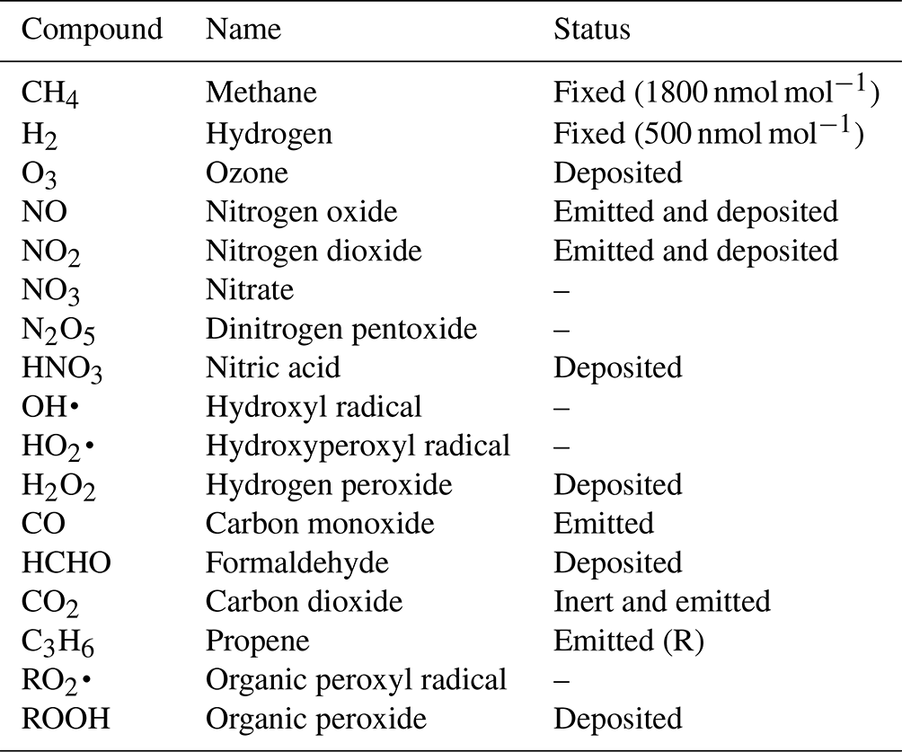
Table 2 Lumping of IFS species into MicroHH tracers. The IFS chemistry scheme is described in Flemming et al. (2015).

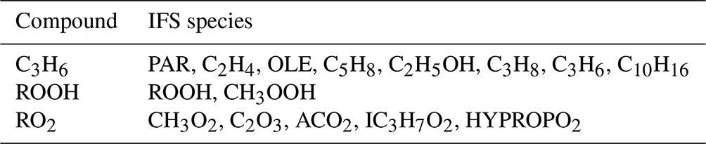
Note: PAR stands for paraffin carbon bond; OLE stands for olefin carbon bond.

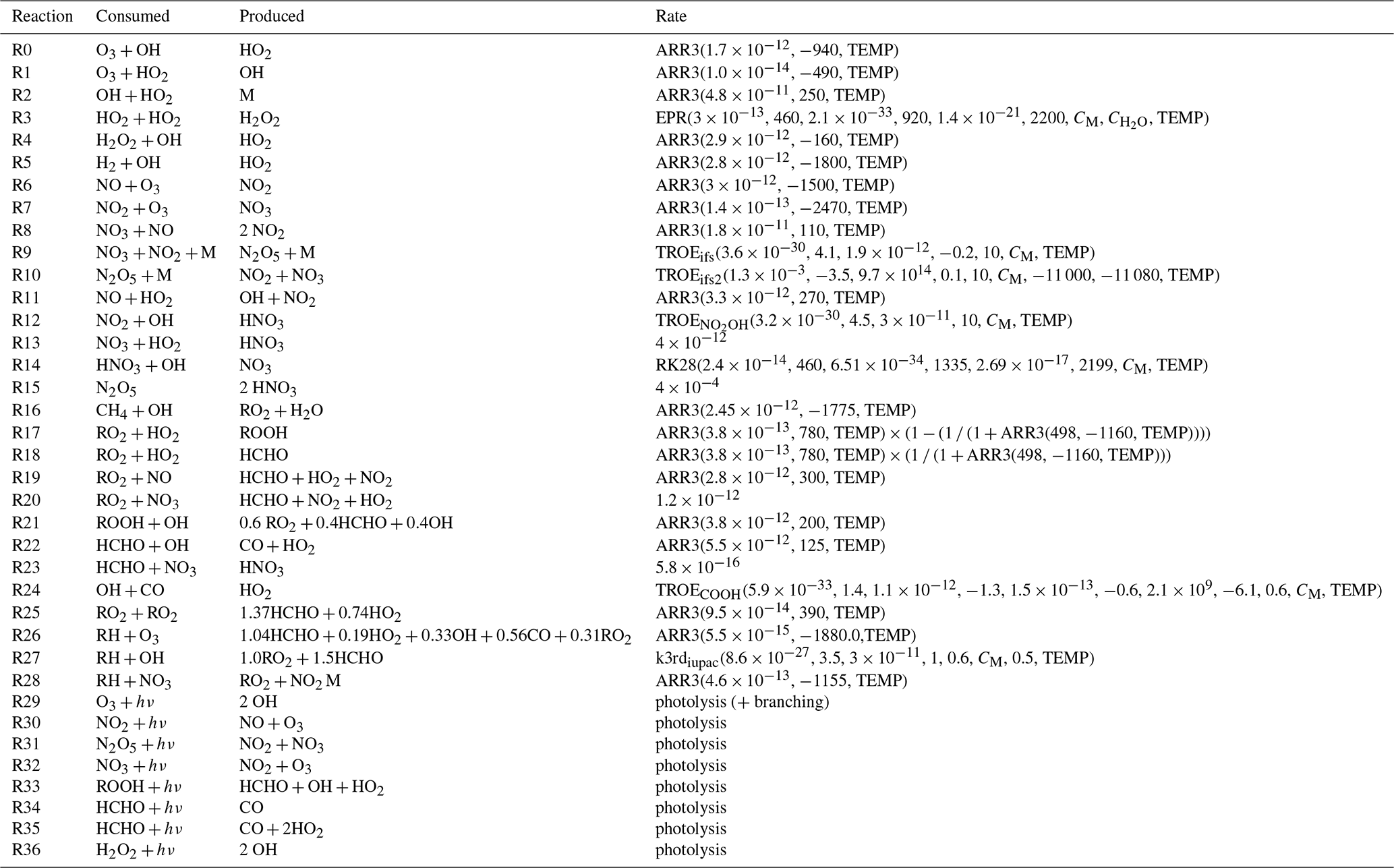
The chemical reactions are generally taken from the IFS chemistry scheme and are listed in Table 3. Note that the reaction scheme also considers surface deposition for HNO₃, O₃, NO, NO₂, HCHO, H₂O₂, and ROOH, as described in Visser (2022). For photolysis frequencies, we produced look-up tables using the Tropospheric Ultraviolet and Visible (TUV) model (Madronich and Flocke, 1998). Here, we took a simple approach using standard atmospheric profiles of aerosol and O₃. We evaluate the photolysis rates at 500 m above the surface with 15 min time steps during a full diurnal cycle for the specific latitude, longitude, and day of the simulation.

Table 3 Reaction scheme employed by MicroHH. M denotes air molecules; hν denotes radiation associated with photolysis; C_M and $C_{{\mathrm{H}}_{\mathrm{2}}\mathrm{O}}$ are the air density and water vapour density, respectively (in molec. cm⁻³); and TEMP is the temperature in kelvin. The rate expressions refer to specific functions to evaluate the rate constants and are taken from the IFS scheme.

To calibrate the reaction scheme to the IFS scheme, we employed a box model implementation of the reduced scheme and compared the results to the full IFS scheme (see Supplement). We performed 2 d simulations with diurnal variation in radiation, representative of an atmospheric boundary layer, and considered two cases. The first case has high emissions of NO and no hydrocarbon emissions. In this case, results of the condensed scheme are nearly identical to those of the IFS scheme (Figs. S1–S3 in the Supplement). Small differences are caused by the omission of, for example, HNO₂ in the condensed scheme. In the second case, we additionally considered emissions of hydrocarbons, represented by C₃H₆. Figure 1 shows the results for some main atmospheric species. Results of additional scenarios are presented in Figs. S1–S9. Note that we tuned the reaction products of Reaction (R27) (1.0RO₂+1.5HCHO) to obtain favourable comparisons for mainly NO₂. Results for HCHO deviate because the condensed scheme does not consider aldehydes, and produces formaldehyde instead (Reaction R27). We consider the comparison with the full IFS scheme favourable and fit for purpose and proceed with a description of the numerical implementation of this chemistry scheme in MicroHH.

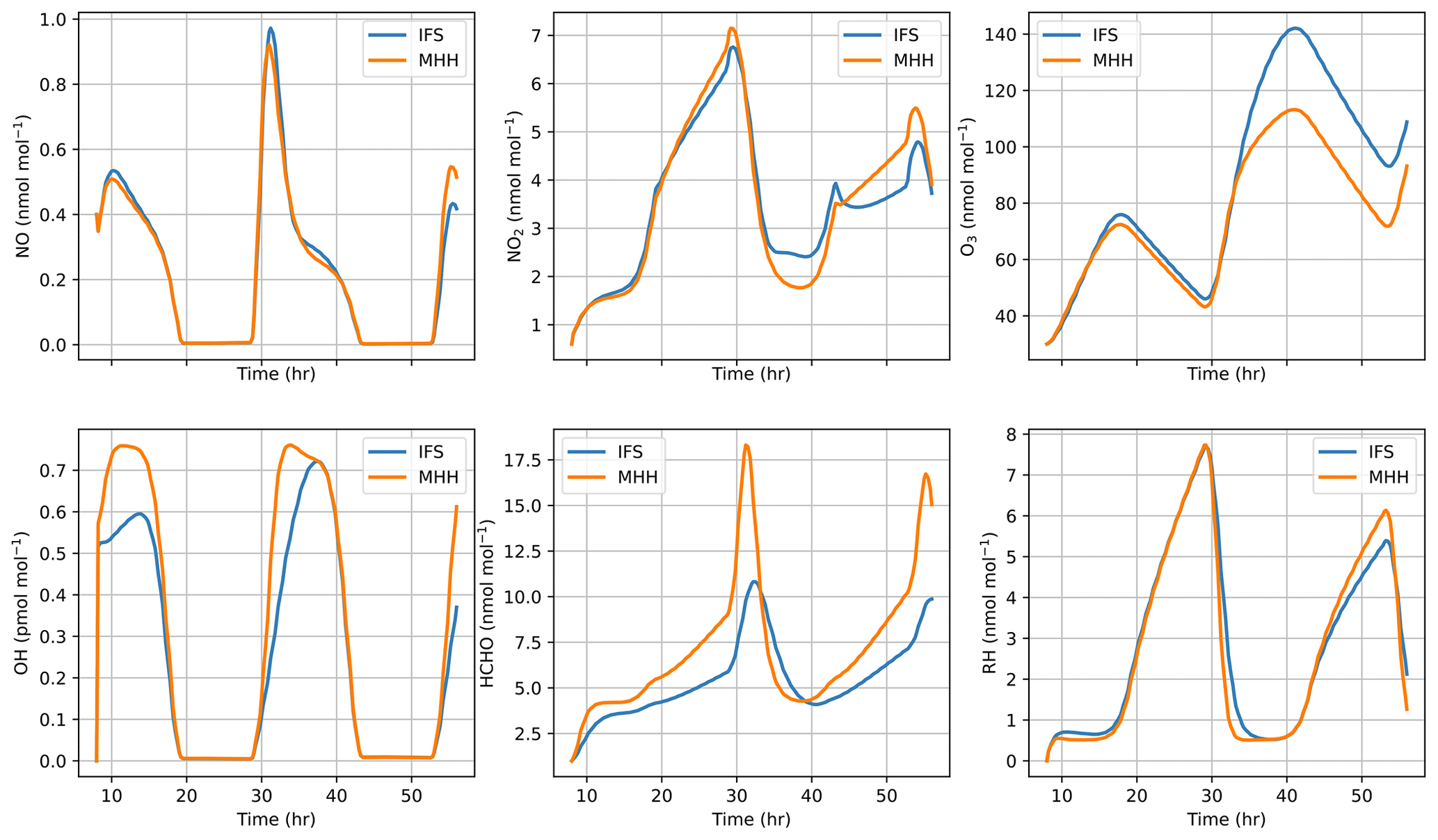
Figure 1 Box model comparison of the IFS scheme with the condensed MicroHH (MHH) scheme. Results of a 2 d simulation are shown with high emissions of NO and C₃H₆, starting at 08:00 LT​​​​​​​. Time series are plotted for NO, NO₂, O₃, OH, HCHO, and RH (C₃H₆).

2.1.2 Numerical implementation

Tracers in MicroHH (van Heerwaarden et al., 2017) are advected using a second-order scheme with a fifth-order interpolation with an imposed flux limiter to ensure monotonicity. Time is advanced with a third-order Runge–Kutta scheme (RK3). During time integration, MicroHH collects tendencies (e.g. advection, cloud processes, and surface exchange) for all meteorological variables and chemistry tracers. Tendencies for tracer emission, deposition, and chemistry are added to these tendencies. Tendencies of chemistry and deposition are evaluated with code that is automatically generated in C-language by the kinetic preprocessor (KPP) (Damian et al., 2002). This code integrates the chemistry rate equations (including deposition terms) from time t to t+dt using the highly accurate Rosenbrock solver. An accurate solver for chemistry is required, because the chemistry rate equations can be very stiff due to the fast timescales involved.

After this integration, which is performed for each of the three sub-steps of the RK3 scheme, tendencies for concentration C are evaluated as follows:

$$\begin{array}{}\text{(1)}& {\left[{\displaystyle \frac{\partial C}{\partial t}}\right]}_{\mathrm{chemistry}}={\displaystyle \frac{C(t+\mathrm{d}t)-C\left(t\right)}{\mathrm{d}t}}.\end{array}$$

The calculation of the chemistry tendencies is evaluated after the calculation of all other tendencies, like advection and emission tendencies. The concentration C(t) before the start of the chemistry integration is updated by these tendencies as follows:

$$\begin{array}{}\text{(2)}& C\left(t\right)=C\left(t\right)+\mathrm{d}t\times {\left[{\displaystyle \frac{\partial C}{\partial t}}\right]}_{\mathrm{other}\mathrm{processes}},\end{array}$$

where dt is the sub-time-step of the RK3 integration (van Heerwaarden et al., 2017). After evaluation, the tendencies are added to the tendencies of the other processes in the main time-integration scheme in MicroHH (van Heerwaarden et al., 2017):

$$\begin{array}{}\text{(3)}& {\displaystyle \frac{\partial C}{\partial t}}={\left[{\displaystyle \frac{\partial C}{\partial t}}\right]}_{\mathrm{other}\mathrm{processes}}+{\left[{\displaystyle \frac{\partial C}{\partial t}}\right]}_{\mathrm{chemistry}}.\end{array}$$

Note that this approach leads to many calls of the Rosenbrock solver (three calls per full time step), which makes the numerical integration of chemistry slow. We found, however, that compromises in the numerical integration lead to numerical instabilities that may result in negative concentrations. In high-resolution simulations of large point sources, large spatial gradients will occur, which are a likely cause of these numerical instabilities. Stack emissions are introduced in the model as described in Ražnjević et al. (2022b). To avoid numerical inaccuracies, point sources are emitted as 3D Gaussian functions that cover four grid boxes in each dimension. Note that this leads to a slight “pre-dispersion” of point sources.

2.2 Simulated cases

One of the aims of the CoCO2 project (https://coco2-project.eu/) is to build a library of plumes. To that end, simulation protocols have been designed (https://coco2-project.eu/sites/default/files/2021-07/CoCO2-D4.1-V1-0.pdf, last access: 10 July 2024). Here, we present results of four cases listed in Table 4 that address emissions from point sources.

Table 4 Simulation cases presented in this paper.

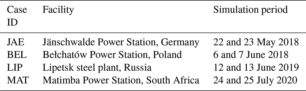
The Jänschwalde Power Station (JAE) is a coal-fired power station near Cottbus, Germany, close to the Germany–Poland border. The Jänschwalde Power Station has nine cooling towers (120 m high) in groups of three, of which only two towers per group are active. This facility has been studied in a couple of recent papers (Brunner et al., 2023; Kuhlmann et al., 2021; Beirle et al., 2021).

The Bełchatów Power Station (BEL) is also a coal-fired power station near Bełchatów, in central Poland. Emissions are released from two 299 m high stacks. CO₂ emissions from this facility have been addressed in Cusworth et al. (2021) and Nassar et al. (2021).

The Lipetsk steel plant (LIP) is owned by the NLMK group, the largest steelmaker in Russia. This facility has been identified in earlier studies (Nassar et al., 2021; Reuter et al., 2019).

Finally, the Matimba Power Station (MAT) is a dry-cooled, coal-fired power plant in the north-east of South Africa, approximately 300 km north of Johannesburg. The power plant has two 250 m high stacks. This case is based on Hakkarainen et al. (2021) and is also addressed in publications such as Hakkarainen et al. (2023), Reuter et al. (2019), and Brunner et al. (2023).

Table 5 Emission configuration of the different simulations. Emissions are distributed vertically, either as a probability density function (JAE and BEL) or as a prescribed distribution. In the former case, emission height and 1σ values are given based on a plume rise calculation. In the latter case, we list the peak emission height and the percentage of the emissions emitted at that height. For JAE and BEL, emissions are evenly distributed over the towers. Emission amounts and heights are taken from the modelling protocols (https://coco2-project.eu/sites/default/files/2021-07/CoCO2-D4.1-V1-0.pdf).

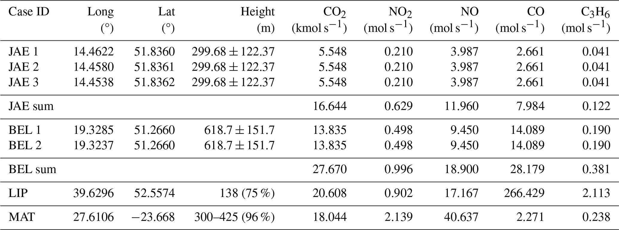
Emission details of these four cases are summarised in Table 5. These facilities are all major emitters of CO₂, with emission strengths ranging from 16 to 28 kmol s⁻¹. For chemical compounds, Matimba is clearly emitting more NO_x, whereas Lipetsk is a very strong emitter of CO.

The emissions are based on the CoCO2 intercomparison protocol (https://coco2-project.eu/sites/default/files/2021-07/CoCO2-D4.1-V1-0.pdf). For JAE and BEL, these emissions are based on reported yearly total values in the European Pollutant Release and Transfer Register (E-PRTR). For MAT, we use the emissions averaged over the year 2018, based on the monthly reports provided by the responsible company – Eskom (https://www.eskom.co.za, last access: 10 July 2024). For LIP, the emissions are obtained from the 2019 annual report of the NLMK group (https://nlmk.com/en/ir/reporting-center/annual-reports/, last access: 10 July 2024). We have smaller confidence in these emissions, because it remains unclear whether the reported emissions can be fully ascribed to the Lipetsk facility.

Concerning emission heights, we prescribed fixed emission profiles that account for plume rise. For JAE and BEL, these were calculated using the empirical equations recommended by the Association of German Engineers, which are based on the original work of Briggs (1984). Typical stack parameters were obtained from Pregger and Friedrich (2009), considering typical power plant capacities and fuel types, and from site descriptions. For LIP and MAT, the emission heights recommended by the CAMS emission dataset (Kuenen et al., 2022) for the Industry and Public Power sectors were used.

Depending on the wind direction during the selected time periods and visual inspection of the TROPOMI NO₂ plumes, a modelling domain was set up around the point source. JAE, BEL, and LIP were modelled on a 51.2 km × 51.2 km domain, whereas a domain of 102.4 km × 102.4 km was selected for the MAT case. All simulations employed a horizontal resolution of 100 m × 100 m. In the vertical, the domain size was 4000 m, with an equidistant grid of 25 m resolution. We tested the effect of model resolution on the simulation results (see Supplement). We found that the conversion of NO to NO₂ proceeds slower and the NO_x : NO₂ ratios are larger at a finer horizontal model resolution of 25 m. At a resolution of 100 m used here, a substantial instant dilution error is still present, which can lead to errors in simulated NO₂ columns as large as 20 % up to 10 km downwind of the stack.

At the top of the domain, a buffer layer starting at 3250 m was used to damp gravity waves (van Heerwaarden et al., 2017). Radiative transfer was calculated every 60 s using the Radiative Transfer for Energetics (RTE) and Rapid Radiative Transfer Model for Global circulation models applications Parallel (RRTMGP) radiative transfer model (Pincus et al., 2019). At the surface, we employed an interactive land surface model based on HTESSEL (Balsamo et al., 2011). We initialised our simulations using CAMS (composition) and ERA5 (meteorology) using LS²D (van Stratum et al., 2023). During the simulations, boundaries were nudged towards time-varying profiles of CAMS and ERA5. For temperature, humidity, and momentum, circular boundary conditions were used. To avoid re-entering of emissions from the point source, we employed free-outflow conditions for tracers, as described in Ražnjević et al. (2022b). As the current focus is on stack emissions, surface fluxes of CO₂ and other tracers were ignored.

Simulations were performed on the Dutch national supercomputer Snellius, using 1024 cores (8 nodes). Typical run times of the simulations ranged from 2 d (JAE, BEL, and LIP) to 5 d (MAT).

2.3 Observations

We compare the results of our simulations to TROPOMI satellite data. We downloaded level-2 TROPOMI NO₂ data from the Copernicus Open Access Hub (https://scihub.copernicus.eu, last access: 4 September 2023). For consistency, we selected the product that was reprocessed (RPRO) with processor version 2.4.0. For JAE, orbits 3136 (22 May 2018) and 3150 (23 May 2018) were downloaded; for BEL, orbits 3349 (6 June 2018) and 3363 (7 June 2018) were downloaded; for LIP, orbits 8611 (12 June 2019) and 8626 (13 June 2019) were downloaded; and for MAT, orbits 14402 (24 July 2020) and 14416 (25 July 2020) were downloaded. The latter two orbits provide data at nadir on a 5.5 km × 3.5 km resolution, whereas the nadir resolution of the other orbits is 7 km × 3.5 km. The uncertainty in a single TROPOMI tropospheric column due to albedo, clouds, and aerosol amounts to 20 %–30 % (van Geffen et al., 2022; Riess et al., 2022).

Figure 2 displays the tropospheric NO₂ columns in the TROPOMI product on the selected days and on the MicroHH modelling domains. Wind speed and direction as calculated with MicroHH are also shown in the panels. We selected only column retrievals with a quality assurance (QA) value > 0.75.

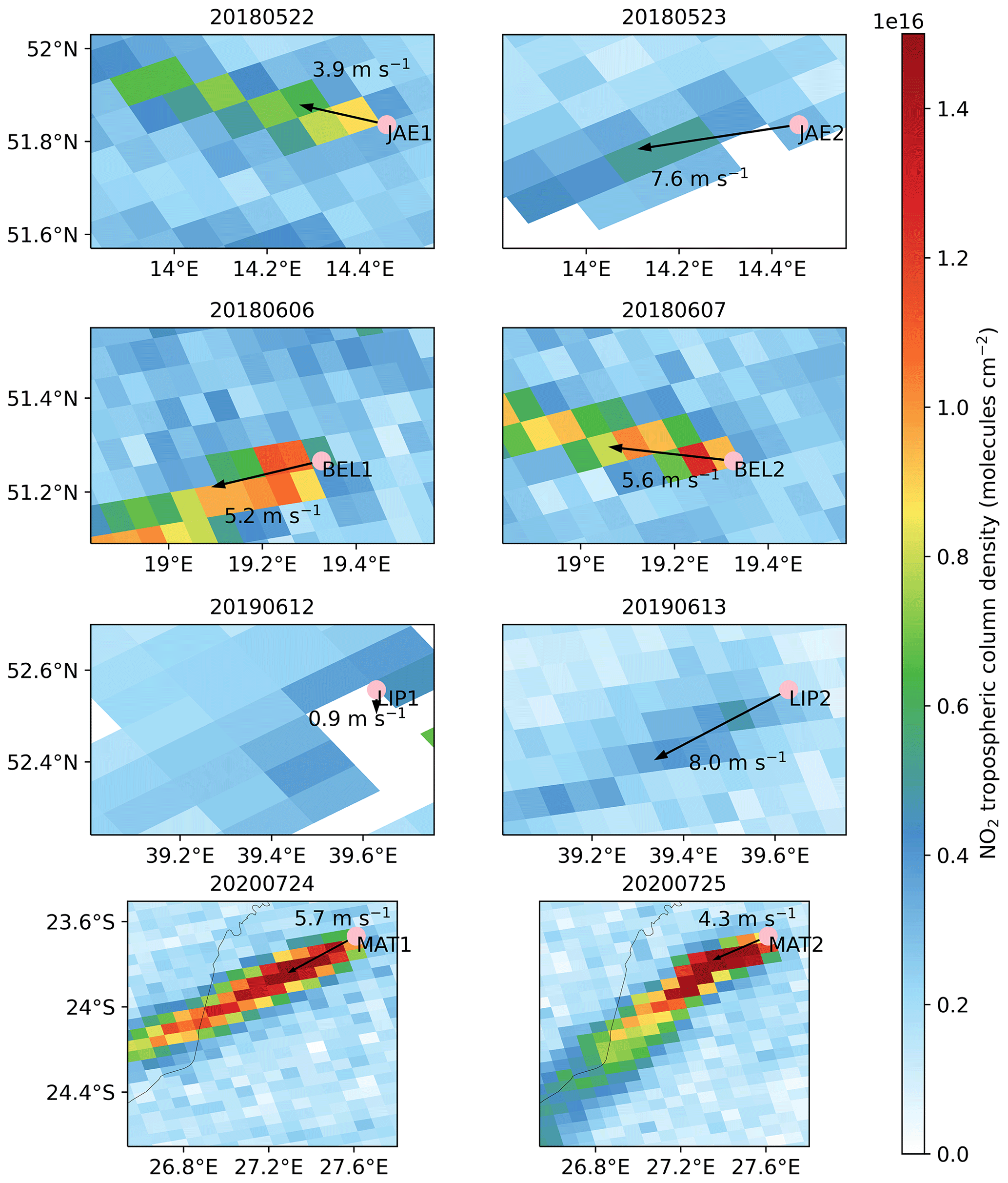
Figure 2 TROPOMI tropospheric NO₂ columns analysed in this paper. Per case, 2 simulation days are considered: the first day is shown in the left column (labelled 1) and the second day in the right column (labelled 2). White pixels refer to TROPOMI sounding with a QA value < 0.75. The central point of emission is labelled by the pink dot. The colour scale is similar for all cases. Note that, for the MAT case, the columns are substantially outside the colour range and the considered domain is twice the size of the other cases. The arrows reflect the domain-averaged wind direction and speed calculated by MicroHH at the TROPOMI overpass time. As will be discussed later, wind speed and direction are weighted in the vertical with the domain-averaged NO₂ profile.

First, the resolution of the TROPOMI product strongly depends on the satellite viewing angle. Second, for all cases, clear NO₂ plumes are visible. Only for the LIP case on 12 June 2019 is the spread of the plume limited due to low wind speeds. Moreover, many TROPOMI pixels are flagged on this day, likely due to aerosol and/or clouds. Finally, as expected and analysed later, the TROPOMI NO₂ columns depend strongly on the wind speed. A clear effect of wind speed is seen on the second day of the JAE case (23 May 2018), when columns are clearly reduced compared with the first day (22 May 2018).

In the further analysis of TROPOMI data, we will remove inconsistencies in the model–satellite comparison caused by the use of vertical NO₂ profiles from the coarse-grid TM5 model in the satellite product. This global chemistry transport model runs on a resolution of 1° × 1° and does not resolve the highly localised plume simulated by MicroHH. As the sensitivity of the satellite measurement drops significantly for NO₂ that resides near the surface, mainly due to Rayleigh scattering, it is important to correct for the differences in NO₂ profile shape and NO₂ amount between MicroHH and TM5. Previous studies have shown strong impacts of the NO₂ profile and amount on satellite retrievals (Vinken et al., 2014; Visser et al., 2019).

The TM5 information about the vertical NO₂ distribution is stored in the TROPOMI data product in the form of a tropospheric averaging kernel (AK) and air mass factor (AMF). We employ the method outlined in Boersma et al. (2016) and applied in Visser et al. (2019) for the Ozone Monitoring Instrument (OMI). To this end, we sample the MicroHH NO₂ profile, augmented with the CAMS profile above 4 km, on the pressure grid of the TM5-based tropospheric AK, and calculate a correction to the tropospheric AMF as follows:

$$\begin{array}{}\text{(4)}& M_{\mathrm{trop},\mathrm{MHH}}=M_{\mathrm{trop},\mathrm{TM}\mathrm{5}}\times {\displaystyle \frac{{\sum }_{l=\mathrm{1}}^L{A}_{\mathrm{trop},l}{x}_{l,\mathrm{MHH}}}{{\sum }_{l=\mathrm{1}}^L{x}_{l,\mathrm{MHH}}}}.\end{array}$$

Here, M_trop is the tropospheric AMF of the MicroHH model (MHH) or the TM5 model (stored in the satellite product), A_trop,l is the tropospheric averaging kernel element for layer l (also stored in the satellite product), x_l,MHH is the modelled NO₂ column density sampled on the TM5 pressure grid, and L is the uppermost TM5 layer in the troposphere. In Sect. 3.3, we will compare MicroHH tropospheric NO₂ columns to corrected and uncorrected TROPOMI tropospheric NO₂ columns.

3 Results

In the following sections, we will present results of the simulations. We start with descriptions of the meteorological characteristics of the four cases, specified for the time around the TROPOMI overpass. Next, we will analyse the chemistry in the plumes with a focus on the NO₂ lifetime and the NO_x:NO₂ ratio. Here, we will compare the simulated CO₂ plumes to the simulated NO₂ plumes. Finally, we will compare the simulated NO₂ plumes to TROPOMI observations.

3.1 Meteorology

Simulations started at 00:00 UTC and lasted for 48 h. Figure 3 shows the simulated wind speeds below 1000 m, averaged over the model domains. Also indicated are the TROPOMI overpass times. These wind speeds are strongly determined by the boundary conditions that are provided by ERA5. Driven by the synoptic situation, winds in the lower boundary layer vary considerably. We often observe a slowdown of the wind prior to TROPOMI overpass (vertical lines). This is related to the growing convective boundary layer in the morning that propagates surface friction to higher altitudes. For LIP, winds are calm prior to the TROPOMI overpass on day 1, whereas the wind speed increases to more than 8 m s⁻¹ prior to the TROPOMI overpass on day 2. This is clearly reflected in the TROPOMI data in Fig. 2. Likewise, the lower TROPOMI columns for JAE on the second day are caused by the higher wind speeds on day 2.

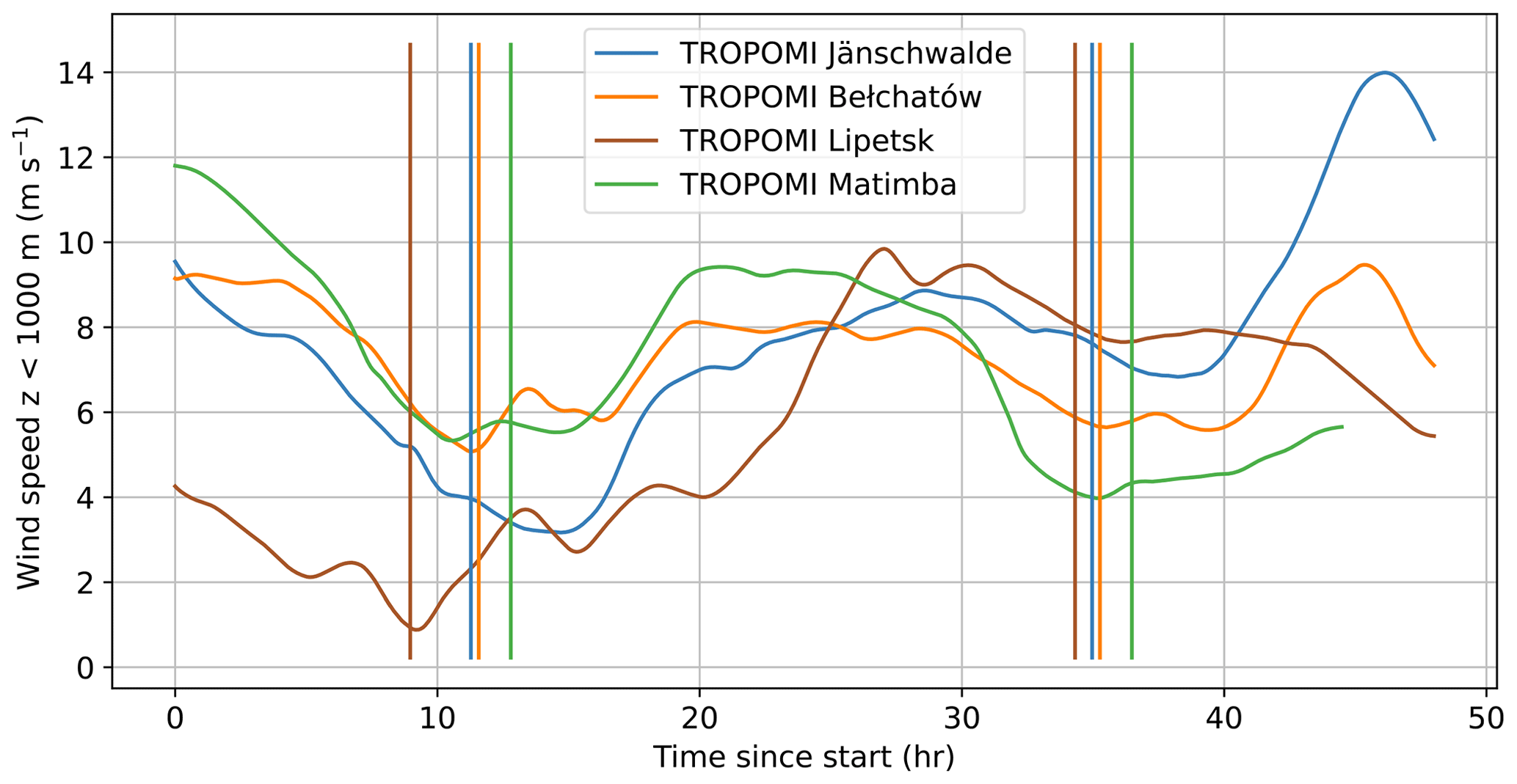
Figure 3 Time variation in the average wind speed at altitudes lower than 1000 m, horizontally averaged over the MicroHH model domains (Fig. 2). The vertical lines denote the UTC time of the TROPOMI overpass on the 2 simulated days for each case.

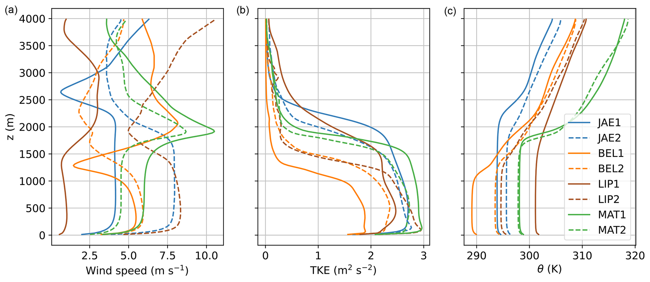
Figure 4 Domain-averaged profiles of wind speed (a), turbulent kinetic energy (TKE, b), and potential temperature (θ, c) averaged 30 min around the TROPOMI overpass. Solid lines are for day 1 of the simulated cases, while dashed lines are for day 2.

To analyse the situation further, Fig. 4 shows profiles of wind speed, turbulent kinetic energy (TKE), and potential temperature (θ) sampled 30 min around the TROPOMI overpasses. TKE (m² s⁻²) is calculated from the variances of the three wind components:

$$\begin{array}{}\text{(5)}& \mathrm{TKE}={\displaystyle \frac{\mathrm{1}}{\mathrm{2}}}\left({\mathit{\sigma }}_u^{\mathrm{2}}+{\mathit{\sigma }}_v^{\mathrm{2}}+{\mathit{\sigma }}_w^{\mathrm{2}}\right).\end{array}$$

In all cases, a well-mixed boundary layer is visible up to the inversions layer, with logarithmic profiles close to the surface. For instance, the boundary layer depth of the JAE1 case amounts to roughly 2500 m. We expect that, due to convective mixing, emissions from the stack will be distributed over the well-mixed boundary layer. Above the inversion layer wind speeds either increase or decrease, while the wind directions change considerably with height (not shown). Despite the low wind speed, TKE is substantial in the Lipetsk day-1 (LIP1) case, pointing to strong buoyancy. Turbulent mixing within the boundary layer is smallest in the Bełchatów day-1 (BEL1) case.

To derive a representative wind direction for plume dispersion, we determine this direction by weighting the wind-profile with the mean NO₂ profile. We subsequently rotate the MicroHH domain around the stack location using the plume direction angle, shown in Fig. 2, such that the plumes are aligned along the positive x axis.

3.2 Plume chemistry

Figure 5 displays the simulated NO₂ mole fractions, averaged over the boundary layer at the times of TROPOMI overpass (see Fig. 3). All plumes are aligned along the x axis and share the same colour scale. Except for the LIP1 simulation, which will be excluded in further analyses, the plumes stay within the Gaussian-type plume depicted by the black lines, which indicates that the winds are relatively stable in direction. The NO₂ abundance in the plume is mostly determined by the emission strength and the wind speed. However, as will be shown later, chemistry also plays and important role. The Jänschwalde day-1 (JAE1) and Bełchatów day-2 (BEL2) plumes show more wavy lateral displacements compared with the other plumes, while the Matimba plumes reveal a slight curvature, possibly due to effects of the Coriolis force (Potts et al., 2023).

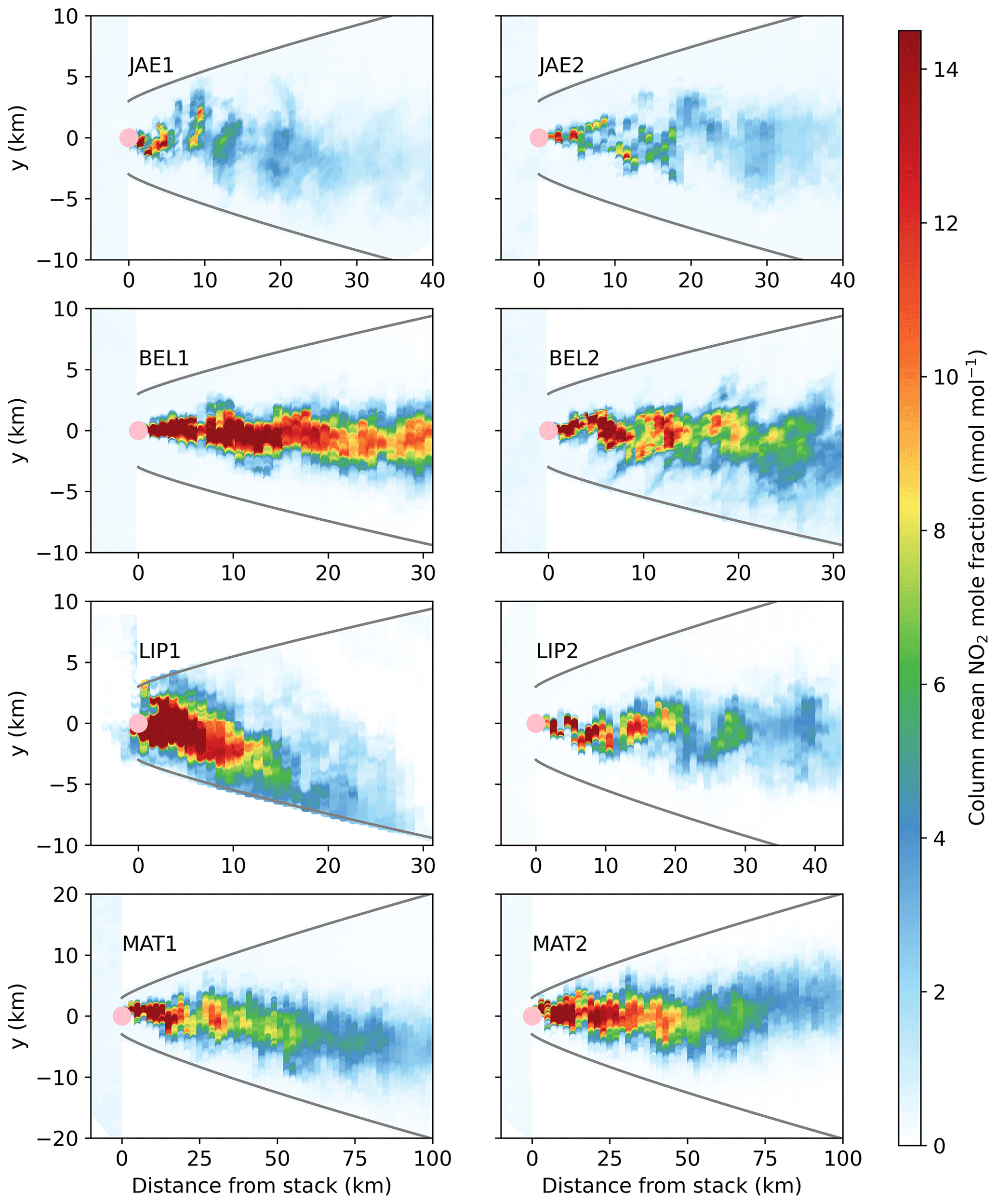
Figure 5 Simulated z-averaged NO₂ mole fraction of the simulated plumes at the TROPOMI overpass time, aligned along the x axis. The pink dots indicate the stack location. Mole fractions have been averaged between the surface and the height of the boundary layer. These boundary layer heights are 2500 (JAE1), 2000 (JAE2), 1200 (BEL1), 1500 (BEL2), 1800 (LIP1), 1500 (LIP2), 1900 (MAT1), and 1850 m (MAT2), respectively, and are derived from Fig. 4. The black solid lines that encapsulate the plumes represent a Gaussian-type plume shape and are given by the equation $y=\pm (\mathrm{3000}+\mathrm{1.08}\times x^{\mathrm{0.84}})$, with x and y in metres. Note that the x and y axes have different scales in the different panels.

To investigate the chemistry in the plume, cross-sections up- and downwind of the stacks are analysed for the NO₂ and NO_x lifetime, the mixing of NO₂ within the plume, and the abundance of OH. For all plume slabs downwind of the stack, averages are taken within the Gaussian-shape black lines in Fig. 5 and bounded by the height of the boundary layer. Outside the plume upwind of the stack, the full domain up to the boundary layer height is considered. The lifetimes of NO_x and NO₂ are calculated by moles of NO_x (NO + NO₂) or NO₂ (mol) divided by NO₂ loss in the reaction between NO₂ and OH (mol s⁻¹). The mean OH mole fraction represents the volume mean OH in these slabs. The mixing of NO₂ is quantified by calculating the intensity of segregation between OH and NO₂ in the slabs, which is defined as follows:

$$\begin{array}{}\text{(6)}& I_{\mathrm{s},{\mathrm{NO}}_{\mathrm{2}},\mathrm{OH}}={\displaystyle \frac{\stackrel{\mathrm{‾}}{\left({\mathrm{NO}}_{\mathrm{2}}-\stackrel{\mathrm{‾}}{{\mathrm{NO}}_{\mathrm{2}}}\right)\left(\mathrm{OH}-\stackrel{\mathrm{‾}}{\mathrm{OH}}\right)}}{\stackrel{\mathrm{‾}}{{\mathrm{NO}}_{\mathrm{2}}}\stackrel{\mathrm{‾}}{\mathrm{OH}}}}.\end{array}$$

Here, the bar represents a volume average. Thus, I_s represents the scaled covariance between two reactive compounds in a volume (Danckwerts, 1952; Vilà-Guerau de Arellano et al., 1990; Galmarini et al., 1995; Krol et al., 2000; Ouwersloot et al., 2011). Generally, a negative value of I_s signals a situation in which the concentrations of two reactants are negatively correlated, which implies that the chemical reaction between these species proceeds more slowly compared with a well-mixed situation. In contrast, a positive value of I_s indicates that the reacting species are spatially correlated in a volume.

Thus, the I_s concept quantifies the effect of assuming a well-mixed situation, e.g. in coarse-grid models. Specifically, if $k_{{\mathrm{NO}}_{\mathrm{2}},\mathrm{OH}}$ represents the reaction rate between NO₂ and OH under well-mixed conditions, the modified reaction rate in a heterogeneously mixed air volume becomes the following:

$$\begin{array}{}\text{(7)}& k_{{\mathrm{NO}}_{\mathrm{2}},\mathrm{OH}}^{\prime }=k_{{\mathrm{NO}}_{\mathrm{2}},\mathrm{OH}}\times \left(\mathrm{1}+I_{\mathrm{s},{\mathrm{NO}}_{\mathrm{2}},\mathrm{OH}}\right).\end{array}$$

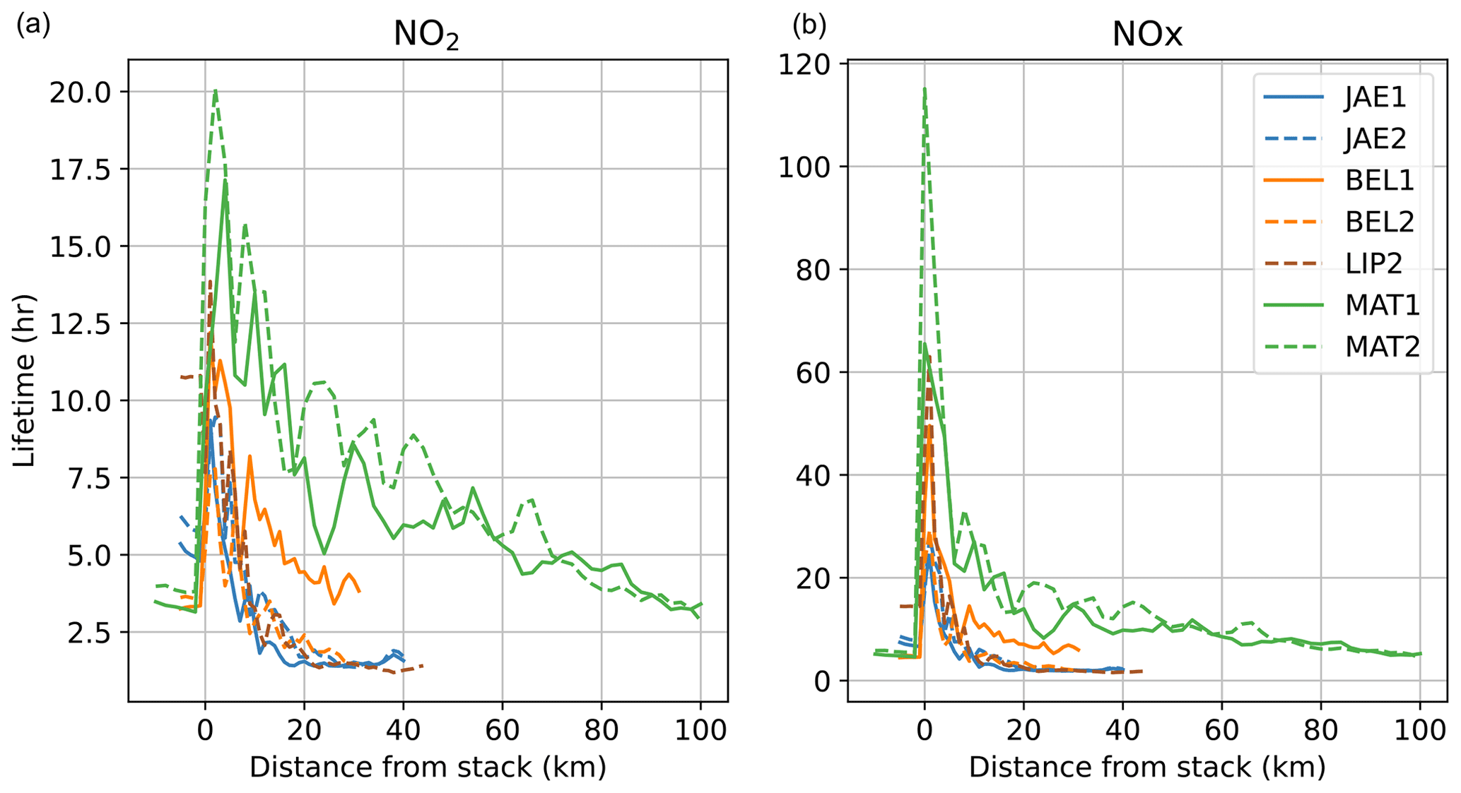
Figure 6 NO₂ (a) and NO_x (b) lifetimes in the simulated plumes at the time of TROPOMI overpass, excluding LIP1. Lifetimes are calculated in volumes determined by 1 km slabs in the x direction, the distance enclosed by the black lines in Fig. 5 in the y direction, and the height of the boundary layer (see caption of Fig. 5). Lifetimes are defined as moles of NO₂ or NO_x (NO + NO₂) (mol) in this volume divided by the chemical loss of NO₂ through the NO₂–OH reaction (mol s⁻¹) in the same volume.

Figure 6 shows the calculated lifetimes of NO₂ (panel a) and NO_x (panel b) in the simulated plumes. Figures S15 and S16 show the lifetimes of NO₂ and NO_x degraded to the TROPOMI resolution. Right after emission, lifetimes show a clear spike. This is caused by the switch from a low or intermediate chemical NO_x regime to a high-NO_x regime in the plume (McKeen et al., 1997; Vinken et al., 2011; Edwards et al., 2017; de Gouw et al., 2019). In this regime, NO₂ becomes the main sink for OH (Reaction R12 in Table 3). Moreover, the concentration of O₃ drops to low values because of the reaction between O₃ and NO (Reaction R6 in Table 3). Note that 95 % of the NO_x is emitted as NO.

Further downwind in the plumes, mixing of the plume with ambient air leads to a recovery of the NO_x and NO₂ lifetimes. Even further downwind, lifetimes may become substantially shorter compared with ambient conditions. For instance, NO₂ lifetimes converge to 1.5 h for JAE1, JAE2, BEL2, and LIP2. This shorter NO_x lifetime within the plume corresponds to findings in de Gouw et al. (2019), who report faster removal of hydrocarbons in pollution plumes. The lifetime reduction depends strongly on the strength of mixing and the amount of NO_x that is emitted at the stack. For Matimba, NO_x emissions are very high (Table 5), which leads to a stronger perturbation of the plume chemistry and a slower recovery of the lifetimes. For Bełchatów, the BEL1 plume stays intact longer compared with the BEL2 plume, driven by weaker mixing of the BEL1 plume (Fig. 4). As a result, BEL1, MAT1, and MAT2 lifetimes remain longer than the background over the entire plume length.

Chemically, the behaviour of the lifetimes can be explained by the strong non-linear relation between the NO₂ abundance and its main sink OH. OH levels show a maximum at NO₂ mole fractions of 1–10 nmol mol⁻¹ due to recycling of OH (e.g. Reaction R11) (Ehhalt and Rohrer, 2000; Lelieveld et al., 2002; Valin et al., 2013). Indeed, we observe this relation in our simulations, with low OH in the core plume (high NO_x) and high OH concentrations at the plume edges, where (due to intermediate NO_x levels) OH recycling is efficient.

Figure 7 $I_{\mathrm{s},{\mathrm{NO}}_{\mathrm{2}},\mathrm{OH}}$ (a, in percent) and mean OH (b, in pmol mol⁻¹) as a function of distance from the stack location. Leftmost x values smaller than zero represent background air. For the definition of the volumes that were used for averaging, see Fig. 6. I_s is defined in Eq. (6).

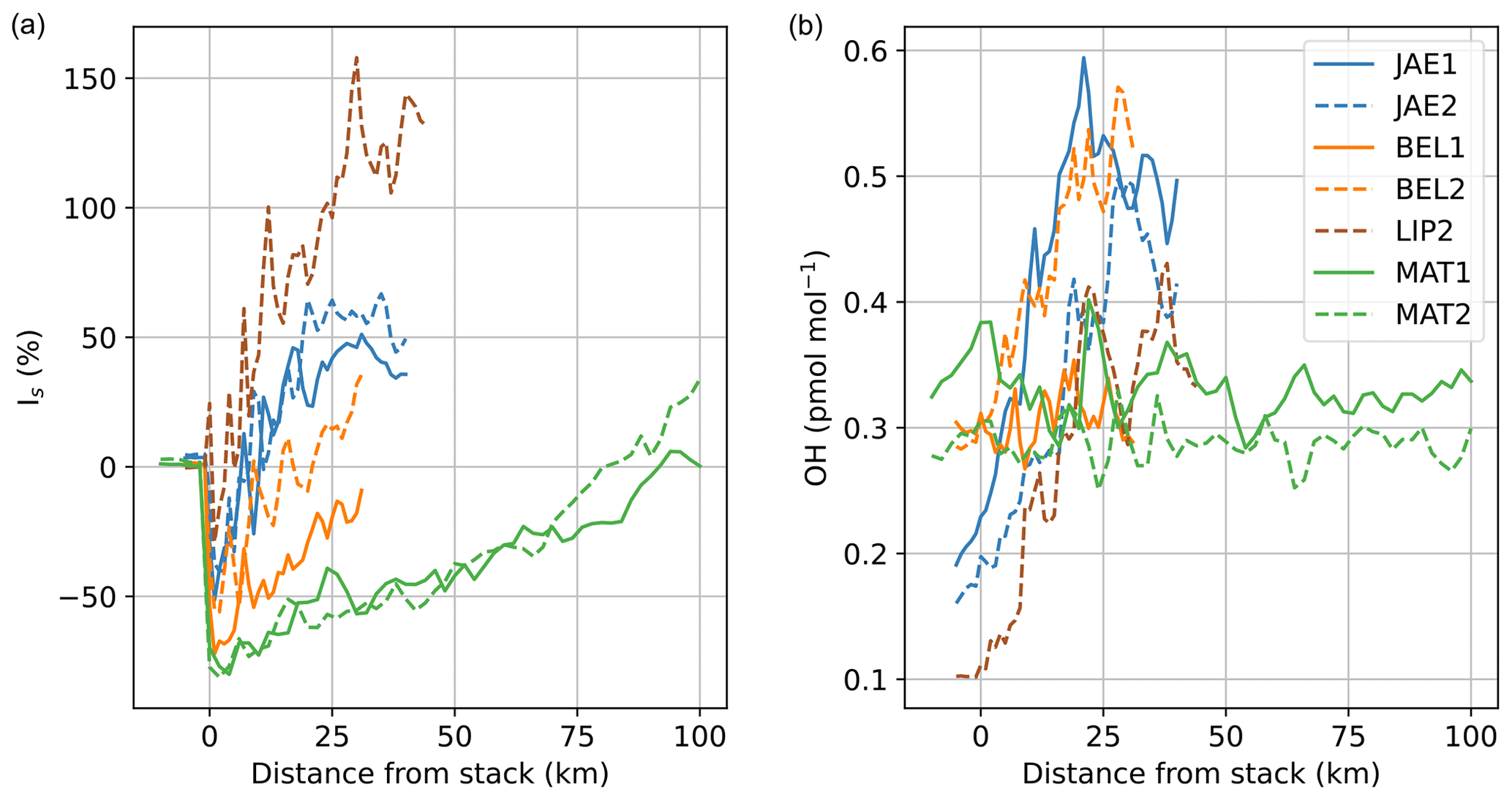
To separate the effects of OH and mixing effects on the simulated lifetimes, Fig. 7 shows slab-averaged $I_{\mathrm{s},{\mathrm{NO}}_{\mathrm{2}},\mathrm{OH}}$ (panel a) and OH (panel b) for the simulations. Figure S17 shows $I_{\mathrm{s},{\mathrm{NO}}_{\mathrm{2}},\mathrm{OH}}$ degraded to the TROPOMI resolution. I_s values vary strongly downwind of the stack. Starting from values close to zero outside the plume, values turn negative first, signalling anti-correlations between NO₂ and OH, in line with the high-NO_x regime. For JAE1, JAE2, BEL2, and LIP2, I_s values turn positive after ≈ 10 km. This implies a positive correlation between NO₂ and OH due to the strong recycling of OH in the chemical oxidation chain (Ehhalt and Rohrer, 2000; Lelieveld et al., 2002; Valin et al., 2013). In contrast, the BEL1, MAT1, and MAT2 plumes show negative I_s values, although values become gradually less negative at larger downwind distances and turn positive for the Matimba case at large distances from the stack. The split between intact and well-mixed NO₂ plumes also appears in mean OH mole fractions. In well-mixed plumes, mean OH in the plume is substantially enhanced further downwind of the stack, while OH stays roughly invariant in the BEL1, MAT1, and MAT2 simulations. For the latter plumes, the enhanced lifetimes (Fig. 6) are therefore mostly determined by I_s, while a combination of higher mean OH and I_s is responsible for the lifetime behaviour in the other plumes. Note that background lifetimes show large variations that are driven by differences in OH values outside the plume. For instance, the background NO₂ lifetime is ≈ 11 h for LIP2, corresponding to an OH mole fraction of ≈ 0.1 pmol mol⁻¹. In contrast, values for MAT1 amount to ≈ 3.5 h and ≈ 0.35 pmol mol⁻¹.

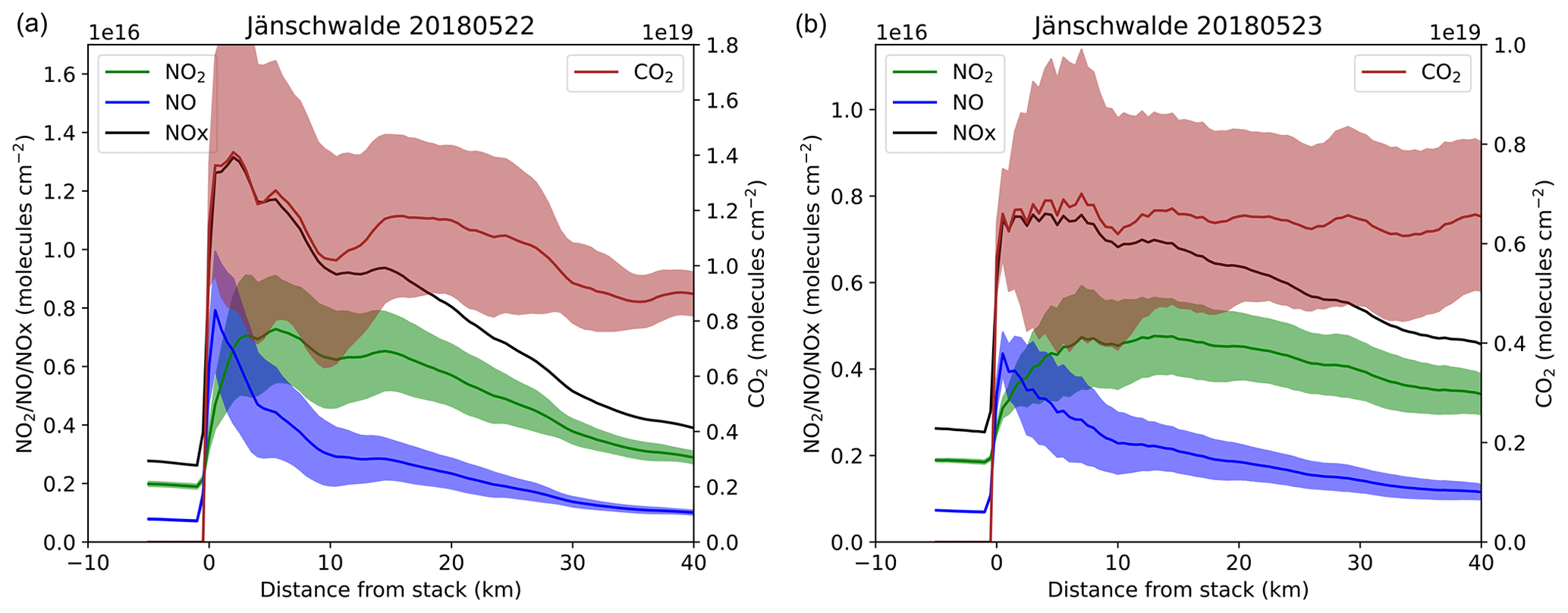
Figure 8 CO₂, NO, NO₂, and NO_x columns up- and downwind of the Jänschwalde stack. Panels (a) and (b) refer to day 1 and day 2 of the simulation, respectively. Columns include the entire modelled column (0–4 km) and are averaged between y = −10 km and y = +10 km. Shaded areas (all species except NO_x) represent the 1σ temporal variability during 1 h around the TROPOMI overpass time. NO, NO₂, and NO_x columns are shown on the left axis, while the CO₂ column is shown on the right axis. Note that the y axes differ for both panels.

In a next step, we connect to methods that have been developed with the aim of quantifying plume emissions from satellite data. For instance, in the cross-sectional flux (CSF) method described by Kuhlmann et al. (2020, 2021), the emission (in mol s⁻¹) is derived from the integrals of the cross-section of the plume perpendicular to the wind direction (i.e. line density in mol m⁻¹) multiplied by an effective wind speed (in m s⁻¹). To investigate the validity of the underlying assumptions in these methods, Fig. 8 shows column densities (0–4 km) of CO₂, NO, NO₂, and NO_x (NO + NO₂), calculated as the mean in the cross-wind direction (y = [−10 km, 10 km], in molec. cm⁻²) on the 2 Jänschwalde simulation days. Columns have been averaged during 1 h around the TROPOMI overpass, and the shaded areas denote 1σ variability (NO, NO₂, and CO₂). To allow comparison to NO_x, the right CO₂ axes have been scaled such that the CO₂ and NO_x maxima match. As a result of the higher wind speed during the second day of the simulation, both y axes in panel (b) have smaller values (Fig. 4).

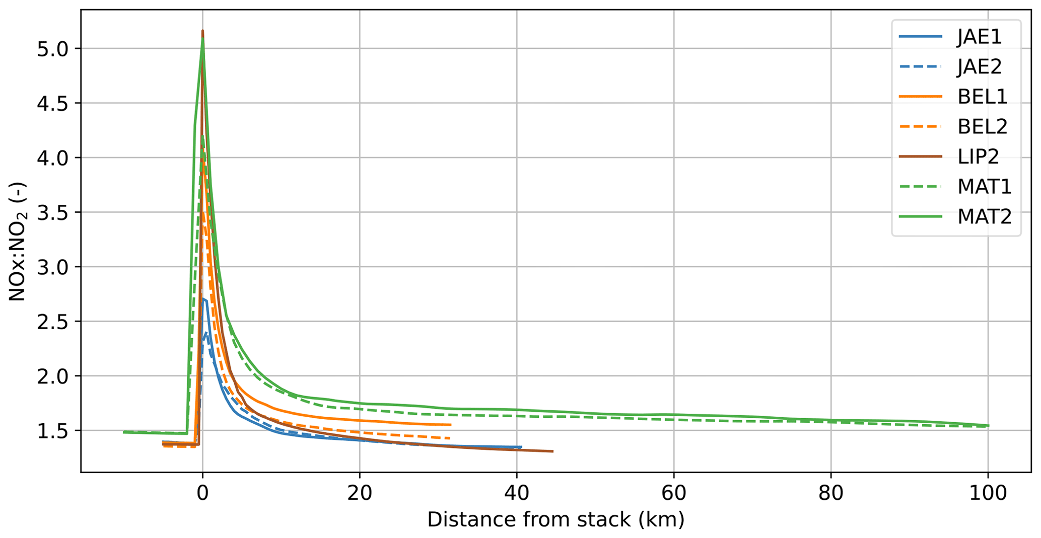
Figure 9 NO_x:NO₂ molar ratios for all simulations. Values are averaged over 1 h around the TROPOMI overpass and for atmospheric slabs up- and downwind of the stack. These slabs extend to model top (4 km) and are averaged over y = [−10 km, +10 km] ([−20 km, +20 km] for MAT).

First, variability in the columns during this sampling hour is large, indicating a large role of turbulence. Due to turbulent eddies that are aligned with the wind direction, downwind transport of species from the stack is irregular, resulting in persistent high-concentration patches that move downwind (e.g. Fig. 5 and Cassiani et al., 2020). Second, variability downwind of the stack decays on day 1 but remains sizable on day 2. Third, CO₂ columns in the plume are not constant on day 1, which shows that the gradual slowing down of the winds (see Fig. 3) has had a noticeable impact on the simulated columns. Assuming a mean wind speed of 5 m s⁻¹ in the atmospheric boundary layer (Fig. 3), the NO_x and CO₂ as sampled 40 km downwind of the stack was emitted more than 2 h prior to the TROPOMI overpass. Fourth, because of chemical removal of NO₂, NO_x columns decay faster than CO₂ columns. Figure 6 shows that this lifetime is not constant but, rather, gets substantially shorter at larger distances from the stack, a feature that also shows up in Fig. 8. Finally, the NO_x:NO₂ ratio varies considerably along the plume. This is further corroborated in Fig. 9, which shows the ratios for all simulations, except for LIP1. Figure S18 shows the NO_x:NO₂ ratio at the TROPOMI resolution.

For all plumes, NO_x:NO₂ ratios quickly rise from a background value of 1.3–1.5 to values of 3–5. Within the first 10 km, values decline to below 2, with further declines to background values further downwind of the stack. Interestingly, the downwind decay of NO_x:NO₂ ratios is slower for BEL1, MAT1, and MAT2, compared with the faster decaying plumes (JAE1, JAE2, BEL2, and LIP2). Thus, slow decaying plumes are characterised by persistent negative values of I_s, longer NO₂ and NO_x lifetimes, and larger NO_x:NO₂ ratios. Both chemical factors (i.e. the size of the perturbation of the background chemistry) and mixing factors (i.e. mixing with ambient air) play a role is determining the plume behaviour.

In the next section, we will compare the simulated NO₂ columns to TROPOMI and evaluate the NO_x emissions that were applied in the simulations.

3.3 Comparison to TROPOMI

As a first comparison between TROPOMI and the simulations, Fig. 10 shows the model results at the TROPOMI overpass time plotted on top of the TROPOMI NO₂ columns. As the simulations are on a 100 m resolution, more detail is visible in the simulations, and the NO₂ columns (even considering only z = 0–4 km) are often outside the maximum colour range. Generally, the simulated plumes align well with the observations. However, for BEL1 and MAT2, the simulated plume direction differs by roughly 10 ° from the observed plume direction. For LIP1, the plume direction is ill-defined due to low wind speeds. Our simulations use meteorological boundary conditions from ERA5, and biases in ERA wind direction have been reported (Sandu et al., 2020). However, the way we impose the ERA5 boundary conditions using one time-dependent profile for the winds, also likely plays a role. As a consequence, when wind curvature is present in the ERA5 forcing fields, this curvature is currently not propagated to the MicroHH simulations. At larger scales, curvature due to the effect of the Coriolis force have been identified in TROPOMI images (Potts et al., 2023).

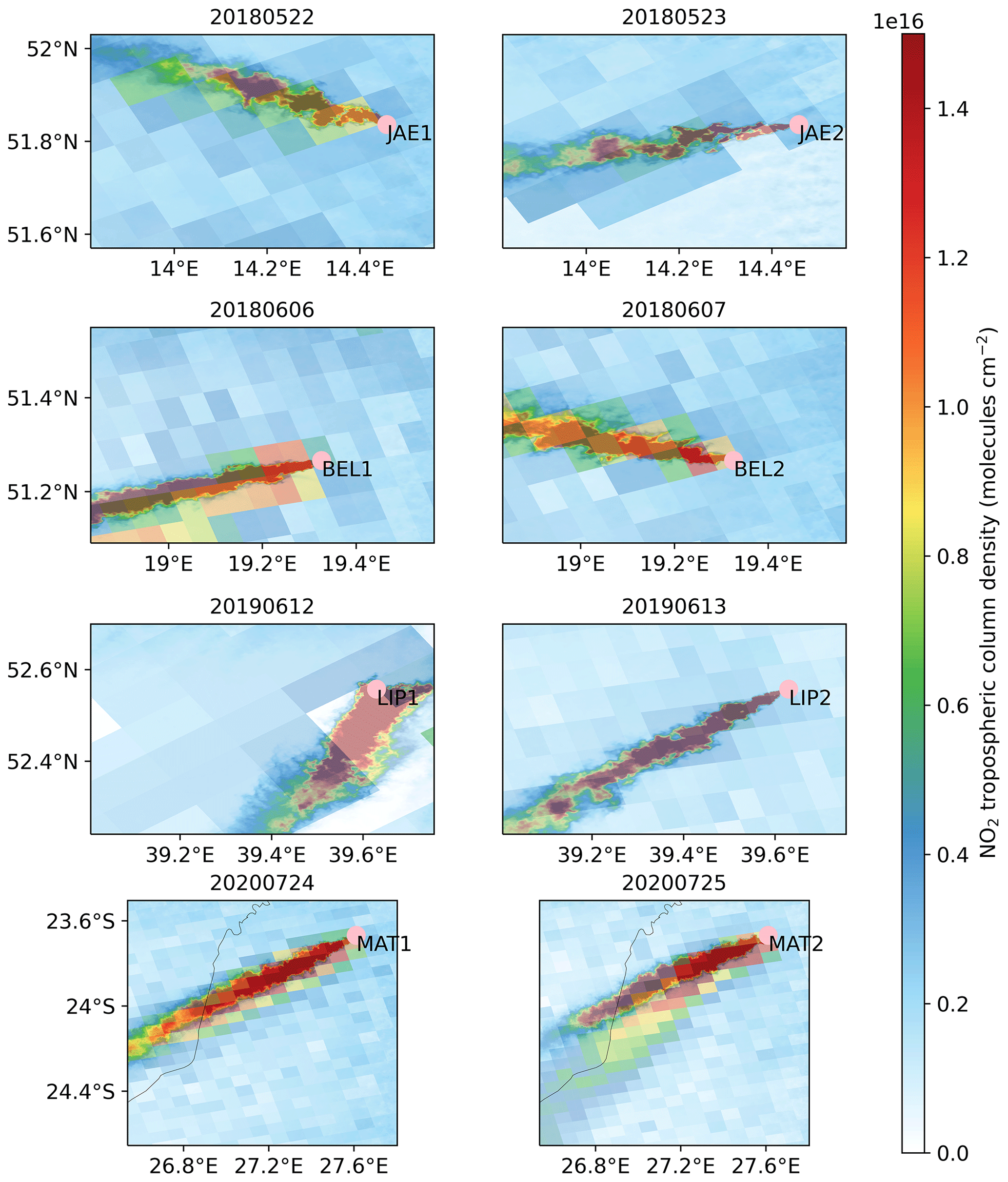
Figure 10 Same as Fig. 2 but now with simulated plumes overplotted on the same colour scale. Note again that, for the MAT case and the simulations, the columns are substantially outside the colour range.

The next steps in the comparison between TROPOMI and simulated NO₂ plumes are a mapping of the simulated NO₂ fields to TROPOMI pixels, an extension of the simulated profiles to the tropopause, and an AMF correction of the TROPOMI columns using Eq. (4). We will present results for the JAE1, JAE2, BEL2, LIP2, and MAT1 cases, based on the favourable match between the model and TROPOMI. We focus on NO₂ enhancements above the background and filter for simulated mean column mole fractions (0–4 km) smaller than 0.28, 0.25, 0.25, 0.15, and 0.28 nmol mol⁻¹ for JAE1, JAE2, BEL2, LIP2, and MAT1, respectively. These values differ slightly per case, because background NO_x and winds vary in the simulations. To compare only the highly concentrated plume, we further discard TROPOMI tropospheric columns smaller than 2 × 10¹⁵ molec. NO₂ cm⁻². To extend the simulated columns to the tropopause, CAMS NO₂ profiles are used. This extension adds a small and relatively constant amount of roughly 0.3 × 10¹⁵ molec. NO₂ cm⁻². As the number of TROPOMI pixels that overlap with the simulated plumes is rather limited (e.g. only ≈ 17 for BEL2), we also use simulated fields 15 min before and after the TROPOMI overpass.

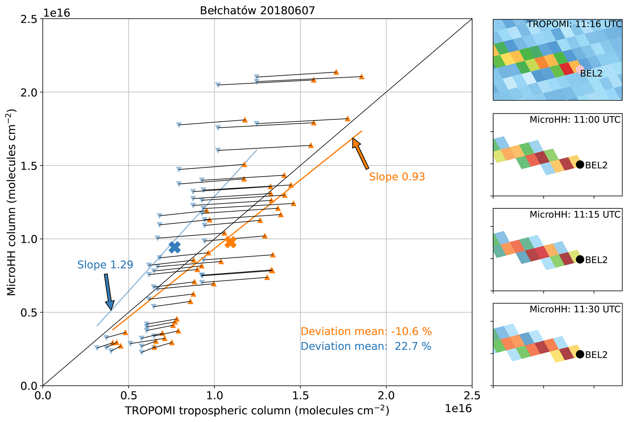
Figure 11 Comparison of simulated and TROPOMI tropospheric NO₂ columns for the BEL2 simulation. The upper right-hand panel repeats the TROPOMI data from Fig. 2. The three panels below are simulation snapshots 15 min apart around the TROPOMI overpass time and are used to account for variations in the turbulent field. The domain and colour bar are the same as in Fig. 2 but in the range of 0–2 × 10¹⁶ molec. cm⁻². These fields are coarsened to the TROPOMI resolution and filtered for enhanced NO₂ mixing ratios to identify the plume (see text). The blue dots and line show comparisons for TROPOMI data that have not been corrected for the AMF (Eq. 4). Moreover, simulated profiles have not been augmented with CAMS NO₂ in the free troposphere (i.e. 0–4 km). The orange dots show the corrected and augmented values, with corrected (orange) and uncorrected (blue) points connected by thin grey lines. Orange and blue lines and slope values represent fits that are forced through the origin. The orange and blue crosses represent the plume-mean columns, and mean deviations ((model − TROPOMI) $/$ TROPOMI in %) are given in the lower right-hand corner.

Figure 11 shows the comparison between TROPOMI and the simulations for the BEL2 case and illustrates the effects of (i) adding free tropospheric columns from CAMS and (ii) the AMF correction of the TROPOMI columns with Eq. (4). The blue points denote the uncorrected TROPOMI NO₂ columns with the uncorrected simulations, while the orange points denote the corrected values. Corrected and uncorrected values are connected with a thin grey line.

When comparing simulations to TROPOMI, it should be realised that the simulations represent a highly turbulent field with large variability (e.g. Fig. 8) and that TROPOMI takes a low-resolution “snapshot” of this turbulent field. A clear one-to-one comparison is therefore not expected. Yet, the integrated or average columns should indicate whether the simulated NO₂ columns are systematically too high or too low. For this reason, we calculated a linear fit (forced through the origin), and the resulting slopes are given in Fig. 11. Moreover, we calculated the mean of the TROPOMI and MicroHH plumes, and results are given by the blue and orange crosses in Fig. 11.

While the uncorrected slope would indicate a 29 % overestimate of NO₂ columns in the simulation (i.e. overly high NO_x emissions), the corrected slope of 0.93 points to a slight underestimate. The change in slope is mostly caused by the AMF correction of the TROPOMI tropospheric NO₂ columns. The correction factor is on average 1.40 (range 1.13–1.68), and corrections are larger for enhanced NO₂ columns. This is caused by the fact that, under polluted conditions, a larger fraction of the NO₂ column resides close to the surface in a high-resolution model like MicroHH, compared with the coarse-scale TM5 model that is used in the TROPOMI product (see Eq. 4). A similar conclusion can be drawn from the plume-mean columns: without correction, MicroHH overestimates the mean TROPOMI column by ≈ 23 %, whereas the mean TROPOMI column is underestimated by ≈ 11 % after correction.

Figure 12 shows the results for all simulations. As for BEL2, the calculated slopes decrease considerably when the AMF correction is applied. Except for LIP2, slopes are within 20 % of the 1 : 1 line, which would indicate that NO_x emissions in the LIP simulation are too high. In Sect. 2.2, we indeed expressed less confidence in the emissions used for the LIP simulation. Results for JAE1 and JAE2 are rather consistent with slopes of ≈ 1.1, while applied emissions for Matimba might be slightly too low. The inset in Fig. 12 shows the plume-mean columns. Again, the AMF correction generally improves the agreement between the simulations and TROPOMI, with signs of overly high (low) emissions for the LIP2 (MAT1) simulation.

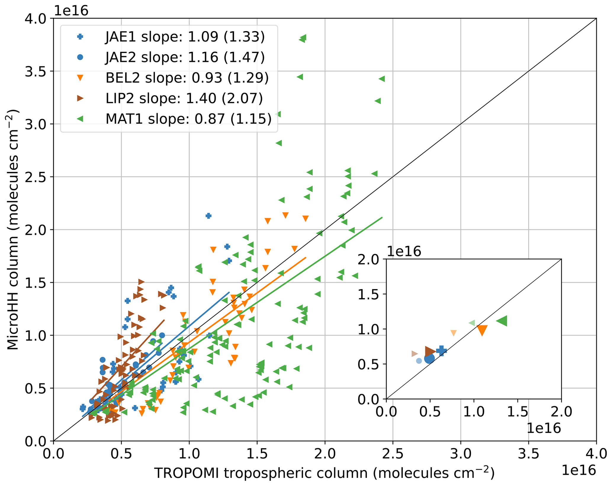
Figure 12 Similar to the main panel in Fig. 11 but now including comparisons for JAE1, JAE2, LIP2, and MAT1. Only corrected TROPOMI and MicroHH results are plotted, and the slope of the fit is given in the legend, with the slope for uncorrected data in parentheses. The inset shows the uncorrected (small transparent) and corrected (big symbols) plume means. Deviations (in %) after (before) correction are +9.3 (+31.5), +17.5 (+46.1), −10.6 (+22.7), +34.3 (+100.4), and −15.3 (+11.3) for JAE1, JAE2, BEL2, LIP2, and MAT1, respectively.

We note, however, that the spread of the individual pixels around the 1 : 1 line is considerable, with systematic model overestimates for high TROPOMI columns and model underestimates for intermediate tropospheric NO₂ columns (specifically for BEL2 and MAT1). This could point to either deficiencies in the model chemistry/transport or to potential biases in the TROPOMI columns. For instance, close to the stack, aerosols and clouds may have influenced the TROPOMI retrievals (Riess et al., 2022; van Geffen et al., 2022). Potential model deficiencies include a rather simple approach for plume rise. For both BEL1 and MAT1, winds aloft are stronger (see Fig. 4) and if plume rise would loft the emissions more, near-stack NO₂ columns would decline while downwind columns would increase, potentially explaining some of the biases in Fig. 12. In general, however, a comparison between a turbulent plume and TROPOMI poses substantial challenges that need to be addressed in the future. For instance, slight rotations or plume-matching algorithms might allow for a more in-depth evaluation of the emissions. For now, we conclude that the emissions that are used in the simulations are likely within 20 % of the true emissions, except for Lipetsk. Deviations might be explained by the use of yearly average emissions in the simulations, while emissions may vary considerably due to varying demand (Kuhlmann et al., 2021; Beirle et al., 2021). In the next section, we will summarise and discuss our main findings.

4 Discussion and conclusions

In this section, we discuss and draw conclusions by addressing the four questions that were posed in the introduction.

4.1 How does atmospheric chemistry affect the NO_x plume?

Our simulations show that large NO_x emissions in a background atmosphere lead to strong non-linear effects, in which the abundance of NO_x strongly influences the NO_x and NO₂ lifetimes, the NO_x:NO₂ ratio, and the duration over which a plume stays chemically intact. This latter effect is most clearly observed for the Matimba simulation in which the largest amount of NO_x is emitted (Table 5). The intensity of segregation between OH and NO₂ ($I_{\mathrm{s},{\mathrm{NO}}_{\mathrm{2}},\mathrm{OH}}$; Eq. 6) stays negative over more than 75 km downwind of the emission point, signalling plume regions that remain in the high-NO_x chemical regime for a long time. Other plumes (JAE1, JAE2, BEL2, and LIP2) show a high-NO_x regime only in the first 5–10 km of the plume. At a larger distance from the stack, a different chemical regime is present, with enhanced OH levels, positive $I_{\mathrm{s},{\mathrm{NO}}_{\mathrm{2}},\mathrm{OH}}$ values, and NO_x and NO₂ lifetimes that are shorter than outside the plume (Fig. 6).

4.2 What is the impact of meteorology on plume dispersion?

Next to the NO_x emission strength, 3D turbulence in the atmospheric boundary layer determines the dynamical and chemical behaviour of the simulated plumes. Although most simulated cases show well-mixed profiles of wind, TKE, and potential temperature in the boundary layer, some plumes are clearly more turbulent than others. For instance, the BEL1 simulation shows less turbulent mixing compared with the BEL2 simulation (Fig. 4). As a result, less ambient air is entrained in the plume, and the plume remains intact for longer, with persistent negative I_s values and longer NO_x and NO₂ lifetimes.

Another important meteorological factor is wind speed. We have identified that wind speed changes affect columns of an inert tracer like CO₂ substantially downwind of the plume (Fig. 8). For instance, the JAE1 simulation shows a substantial slowing down of the wind speed prior to the TROPOMI overpass time (Fig. 3), which increases the CO₂ column by roughly 30 % close to the stack location. To reduce errors in simplified methods that aim to quantify plume emissions from satellite data (Kuhlmann et al., 2020, 2021), these methods should ideally account for these wind speed changes. On top of that, 3D turbulence in the boundary layer leads to large temporal variations in the simulated plumes. Simulated 1σ variations (1 h averaging time) in CO₂ columns can easily reach 30 %, with highest variability close to the stack location. This behaviour of turbulent plumes is well documented (Cassiani et al., 2020; Ražnjević et al., 2022a, b; Mu et al., 2023). Satellite images from polar-orbiting platforms, like TROPOMI and the upcoming CO2M mission (Sierk et al., 2019), take only a snapshot of the turbulent plume, leading to uncertainties in simplified emission estimation methods (Kuhlmann et al., 2020). Large-eddy simulations, as presented in this paper, help to identify the main factors that influence temporal variations in the plume and to design strategies to reduce errors in emission estimation methods.

4.3 How do the simulations compare to TROPOMI NO₂ observations?

Overall, we find a favourable comparison between the simulated plumes and TROPOMI (Fig. 10). The Lipetsk simulation on day 1 had low wind speeds, which makes the comparison with TROPOMI difficult. Two other simulation days, BEL1 and MAT2, show that the simulated plumes are rotated clockwise compared with the observations. Biases in simulated wind direction have been identified as a major source of uncertainty in other studies as well (Hakkarainen et al., 2023, 2019; Wu et al., 2023; Brunner et al., 2023; Zheng et al., 2019; Lin et al., 2023). To allow a direct comparison between simulation and TROPOMI, the implementation of a plume-matching algorithm would be useful (e.g. Kuhlmann et al., 2021). As our simulations are nudged to a single time-dependent wind profile, wind rotation on the synoptic scale can currently not be resolved. Curvature observed in TROPOMI images has been attributed to effects of Coriolis forces (Potts et al., 2023). Efforts are ongoing to embed MicroHH within ERA5 and CAMS on larger domains with spatially varying forcing fields.

One of the largest challenges that has been identified in this study is that temporal variability in turbulent plumes is typically large, making a one-to-one comparison to satellite images difficult. TROPOMI samples in an afternoon orbit (13:30 LT, local time), while CO2M will have an overpass time of 11:30 LT (Sierk et al., 2019). An earlier overpass may avoid some of the strong turbulent plumes that we simulated here. However, other challenges remain.

In a simplified emission estimation procedure, we found that tropospheric TROPOMI columns should be enhanced by ≈ 40 % due to different NO₂ amounts and profile shapes in the simulations (Eq. 4). Also here, however, there is no one-to-one match between a TROPOMI pixel and the simulation, which makes the applied correction uncertain. By averaging over several simulation snapshots 15 min apart and by calculating the plume-mean enhancements, we tried to account for the modelled variability (Fig. 11). Comparisons showed that NO_x emissions used in the simulations were likely correct within 20 %, except for Lipetsk, for which the NO_x emission in the model was ≈ 40 % too high based on the comparison with TROPOMI. However, we also noticed systematic overestimates in the simulated columns close to the emission location and systematic smaller columns at intermediate distances from the stack. Such biases may point to errors in our simplified chemistry and/or TROPOMI retrievals and AMF correction. The latter might be due to the occurrence of plume-generated clouds and aerosol in the stack plume. One interesting finding that needs further exploration is the possible effect of plume rise on the vertical extend of the plume and its subsequent transport in the atmosphere. Simulated wind profiles (Fig. 3) show complex vertical structures. Better characterisation and evaluation of the meteorological situation associated with point source emissions is therefore needed (e.g. Schalkwijk et al., 2015; van Stratum et al., 2023).

4.4 What are the main factors that influence emission quantification from satellite observations?

In the sections above, we identified the main factors that need to be accounted for in simulating plumes and comparison to satellite images.

First, wind speed and direction as well as their variations in space and time drive how plumes are transported after emission. Associated with that, plume emission height and plume rise are important factors that have been identified before (Brunner et al., 2019; Lin et al., 2023).

Second, we found that the NO_x emission strength strongly determines the subsequent fate of the NO_x plume. The large NO_x emissions of the Matimba stack lead to a chemical perturbation that keeps the plume chemically intact for almost 100 km after emissions. Additionally, the turbulent mixing that mixes the plume with ambient air also plays a role, as shown for the Bełchatów simulation. We also identified plumes (JAE1, JAE2, BEL2, and LIP2) that quickly move out of the high-NO_x regime and move into a regime with short NO_x and NO₂ lifetimes. Accounting for proper NO_x lifetimes and NO_x:NO₂ ratios is important to use NO₂ as an additional tracer to constrain CO₂ stack emissions.

Third, the AMF correction of TROPOMI data is an important factor. However, variability in the simulated NO₂ distribution makes a one-to-one comparison to TROPOMI images, and hence a proper AMF correction, difficult. New data-assimilation techniques to better constrain 3D turbulence are being developed (Chandramouli et al., 2020; Bauweraerts and Meyers, 2021) but require time-resolved observations of 3D turbulence. One option to explore is the use of data from recently reported time-resolved imaging spectroscopy (Mu et al., 2023). Our chemistry-enabled MicroHH simulations in combination with these detailed observations may improve methods to quantify emissions from large point sources.

Our study also has some shortcomings. First, our chemistry is simplified and does not account for possible impacts of heterogeneous reactions on aerosol surfaces. In highly concentrated plumes, these processes may be important (Kim et al., 2017). Second, we performed our simulations according to the CoCO2 simulation protocols (https://coco2-project.eu/sites/default/files/2021-07/CoCO2-D4.1-V1-0.pdf) that only crudely account for plume rise. In the future, we could add heat and moisture stack emissions to the simulations to account explicitly for plume rise. Third, next to applying inflow due to CAMS boundary conditions, we only accounted for emissions from the stack, ignoring possible surface emissions. As a result, concentration fields might be less realistic, specifically in the downwind domain outside the plume. Fourth, the use of 100 m resolution LESs at night is insufficient to resolve small-scale turbulence in the nocturnal boundary layer. As a result, transport will be driven by the sub-grid model, leading to an overestimation of mixing. However, the impact on the development of a convective boundary layer on the next day was shown to be limited (van Stratum and Stevens, 2015). As further outlined in the Supplement, a horizontal model resolution of 100 m also proves barely sufficient to properly account for mixing and plume chemistry. Finally, our boundary conditions consist of single time-dependent columns. Thus, the simulations cannot account for commonly observed rotation in the wind fields. Future developments of the MicroHH code will account for these shortcomings. Moreover, we are extending our method to more complicated emission hot spots, like cities.

In general, our simulations provide new insights into the factors that are important for the interpretation of satellite-observed NO₂ plumes. Although it is impractical to run the model for each observed plume, it is likely that the main impacts can be parameterised in light-weight methods, as recently shown in Meier et al. (2024).

In conclusion, we presented LESs of NO₂ plumes from four large emitters world-wide. To this end, we implemented a simple chemistry scheme in the MicroHH model. Simulations showed generally good agreement with TROPOMI images as well as the need to account for the strongly non-linear NO_x chemistry in concentrated plumes. LESs with chemistry are useful to test less-involved algorithms to derive emissions from large point sources. For a start, the use of a fixed NO₂ lifetime and NO_x:NO₂ ratio can be replaced by values derived from our high-resolution plume simulations.