Uncertainty in continuous ΔCO-based ΔffCO₂ estimates derived from ¹⁴C flask and bottom-up ΔCO ∕ ΔffCO₂ ratios

Measuring the ¹⁴C $/$ C depletion in atmospheric CO₂ compared with a clean-air reference is the most direct way to estimate the recently added CO₂ contribution from fossil fuel (ff) combustion (ΔffCO₂) in ambient air. However, as ¹⁴CO₂ measurements cannot be conducted continuously nor remotely, there are only very sparse ¹⁴C-based ΔffCO₂ estimates available. Continuously measured tracers, like carbon monoxide (CO), that are co-emitted with ffCO₂ can be used as proxies for ΔffCO_2, provided that the ΔCO $/$ ΔffCO₂ ratios can be determined correctly (here, ΔCO refers to the CO excess compared with a clean-air reference). In the present study, we use almost 350 ¹⁴CO₂ measurements from flask samples collected between 2019 and 2020 at the urban site Heidelberg, Germany, and corresponding analyses from more than 50 afternoon flasks collected between September 2020 and March 2021 at the rural ICOS site Observatoire pérenne de l'environnement (OPE), France, to calculate average ¹⁴C-based ΔCO $/$ ΔffCO₂ ratios for those sites. For this, we constructed a clean-air reference from the ¹⁴CO₂ and CO measurements of Mace Head, Ireland. By dividing the hourly ΔCO excess observations by the averaged flask ratio, we calculate continuous proxy-based ΔffCO₂ records. The mean bias between the proxy-based ΔffCO₂ and the direct ¹⁴C-based ΔffCO₂ estimates from the flasks is – with 0.31 ± 3.94 ppm for the urban site Heidelberg and −0.06 ± 1.49 ppm for the rural site OPE – only ca. 3 % at both sites. The root-mean-square deviation (RMSD) between proxy-based ΔffCO₂ and ¹⁴C-based ΔffCO₂ is about 4 ppm for Heidelberg and 1.5 ppm for OPE. While this uncertainty can be explained by observational uncertainties alone at OPE, about half of the uncertainty is caused by the neglected variability in the ΔCO $/$ ΔffCO₂ ratios at Heidelberg. We further show that modeled ratios based on a bottom-up European emission inventory would lead to substantial biases in the ΔCO-based ΔffCO₂ estimates for both Heidelberg and OPE. This highlights the need for an ongoing observational calibration and/or validation of inventory-based ratios if they are to be applied for large-scale ΔCO-based ΔffCO₂ estimates, e.g., from satellites.

1 Introduction

The observational separation of the fossil fuel CO₂ contributions (ΔffCO₂) in regional atmospheric CO₂ excess is a prerequisite for independent top-down evaluation of bottom-up ffCO₂ emission inventories (Ciais et al., 2016). The most direct method for estimating regional ΔffCO₂ contributions is measuring the ambient air Δ¹⁴CO₂ depletion compared with a clean-air Δ¹⁴CO₂ reference, as fossil fuels are devoid of ¹⁴C, which has a half-life of 5700 years (Currie, 2004; for the Δ¹⁴CO₂ notation, see Stuiver and Polach, 1977). Many studies have successfully applied this approach to directly estimate regional ΔffCO₂ concentrations in urban regions (Levin et al., 2003; Levin and Rödenbeck, 2008; Turnbull et al., 2015; Miller et al., 2020; Zhou et al., 2020), which could then be used in atmospheric inverse modeling systems for comparison with bottom-up ffCO₂ emission inventories (Graven et al., 2018; Wang et al., 2018). One drawback of this method, however, is that ¹⁴C-based ΔffCO₂ estimates typically only have a low (i.e., weekly or monthly) temporal resolution and poor spatial coverage, due to the labor-intensive and costly process of collecting and precisely measuring air samples for ¹⁴CO₂. Currently, ¹⁴CO₂ observations cannot be conducted continuously with the precision needed for atmospheric ΔffCO₂ determination nor can they be performed remotely, e.g., with satellites. This limits the potential of ¹⁴C observations to estimate ffCO₂ emissions at the continental scale and at high spatiotemporal resolution.

Therefore, more frequently measured gases, like carbon monoxide (CO), which is typically co-emitted with ffCO₂ during incomplete combustion, are being used as an additional constraint for estimating ffCO₂ emissions (e.g., Palmer et al., 2006; Boschetti et al., 2018). Also, CO observations from satellites have shown high potential for verifying and optimizing bottom-up ffCO₂ emission estimates of large industrial regions worldwide (Konovalov et al., 2016). However, using CO observations in inverse models for estimating ffCO₂ emissions requires decent information about the spatiotemporal variability in the CO $/$ ffCO₂ emission ratios. Typically, this information is taken from bottom-up CO and CO₂ emission inventories, which are based on national activity data and source-sector-specific emission factors (Janssens-Maenhout et al., 2019; Kuenen et al., 2022). However, these emission factors are associated with high uncertainties, especially for CO, as they strongly depend on the often variable combustion conditions (Dellaert et al., 2019). Observation-based verification of the bottom-up emission ratios may significantly reduce biases in top-down ffCO₂ emission estimates.

Continuously measured ΔCO offsets compared to a clean-air reference have been used in the past to construct high-temporal-resolution ΔffCO₂ concentration records, which can provide additional spatiotemporal information for constraining fossil emissions in transport model inversions. For this, the continuous ΔCO measurements are divided by mean < ΔCO $/$ ΔffCO₂ > ratios (with mean ratios represented using angle brackets throughout), which are representative of the particular observation site and the averaging period (Gamnitzer et al., 2006; Levin and Karstens, 2007; Van der Laan et al., 2010; Vogel et al., 2010). Note that, in this study, we use the “Δ” in front of “CO” and “ffCO₂” to describe the excess concentrations compared with the clean-air reference; it is different from the Δ notation introduced by Stuiver and Polach (1977) to report ¹⁴CO₂ measurements. At observation sites with simultaneous ¹⁴CO₂ measurements the < ΔCO $/$ ΔffCO₂ > ratios can be calculated from ¹⁴C-based ΔffCO₂ estimates. This allows one to calculate continuous ΔCO-based ΔffCO₂ concentration offsets, which are fully independent of bottom-up emission information and calibrated by Δ¹⁴CO₂ measurements. For example, Turnbull et al. (2011) collected in situ CO₂ and CO measurements as well as Δ¹⁴CO₂ and CO₂ flask samples in the boundary layer and the free troposphere over Sacramento, California, USA, during aircraft flights. They derived an average flask-based < ΔCO $/$ ΔffCO₂ > ratio and combined it with their in situ CO measurements to estimate the ΔffCO₂ concentrations throughout the aircraft flight. By using a mass balance approach, they inferred the ffCO₂ emissions from the Sacramento region, which were comparable to emission estimates from bottom-up inventories. Vogel et al. (2010) used weekly integrated Δ¹⁴CO₂ observations combined with occasional hourly Δ¹⁴CO₂ flask data from the urban site Heidelberg, located in a heavily industrialized area in the Upper Rhine Valley in southwestern Germany, to estimate continuous ΔCO-based ΔffCO₂ concentrations. They show that calculating the ΔCO $/$ ΔffCO₂ ratios from the weekly integrated Δ¹⁴CO₂ samples leads to biases in the ΔCO-based ΔffCO₂ estimates, as the weekly averaged ratios are biased towards hours with high ΔffCO₂ concentrations. That is why they used the Δ¹⁴CO₂ flask data to calculate mean diurnal cycles for the summer and winter periods. By correcting the weekly averaged ratios with these diurnal profiles, they reduced some of the bias in the ΔCO-based ΔffCO₂ estimates.

The basic idea of using ΔCO as a proxy for ΔffCO₂ is more than 20 years old. Even older is the realization that there will be no semicontinuous measurements of the direct ΔffCO₂ tracer Δ¹⁴CO₂ in atmospheric observing networks for the foreseeable future. Thus, the CO proxy approach is a way to bridge the gap between more reliable but sparse ¹⁴C-based ΔffCO₂ estimates with temporal information derived from CO. However, ΔCO is not a perfect ΔffCO₂ proxy for many reasons. Therefore, we consider it the primary goal of this study to clearly emphasize the shortcomings of the CO proxy approach. This includes showing that the use of the CO proxy requires calibration by ¹⁴C measurements to achieve the necessary precision. Despite all of the difficulties and deficits of CO-proxy-based ΔffCO₂ estimation, we will also demonstrate, in this study and in the companion paper by Maier et al. (2024), the great potential of this method.

We have collected almost 350 hourly integrated Δ¹⁴CO₂ flask samples with very different atmospheric conditions at the Heidelberg observation site during 2019 and 2020. In the companion paper (Maier et al., 2024), we show that this large flask pool does not allow for a robust and data-driven estimate of the urban ffCO₂ emissions in the Heidelberg footprint. Our aim in the present study is to assess the use of these hourly Δ¹⁴CO₂ flask data to estimate ΔCO $/$ ΔffCO₂ ratios and then derive a continuous ΔCO-based ΔffCO₂ record for the Heidelberg station, which is calibrated by Δ¹⁴CO₂ measurements. By conducting a synthetic-data experiment (see Sect. 3.1.2), we further estimate the uncertainty in this ΔCO-based ΔffCO₂ record and assess the share of uncertainty that is caused by the spatiotemporal variability in the emission ratios in Heidelberg's surrounding sources. In the companion paper (Maier et al., 2024), we demonstrate that this continuous ΔCO-based ΔffCO₂ record yields robust and data-driven ffCO₂ emission estimates that can be used to investigate the effect of COVID-19 restrictions and to validate the seasonal cycle of a ffCO₂ emission inventory in the main footprint of Heidelberg. To test this approach at a more remote site, a similar investigation is conducted at a rural Integrated Carbon Observation System (ICOS; Heiskanen et al., 2022) atmosphere station, Observatoire pérenne de l'environnement (OPE), but using only about 50 hourly integrated flask samples collected between September 2020 and March 2021 (Sect. 3.2).

We further compare the flask-based ΔCO $/$ ΔffCO₂ ratios with modeled ratios based on bottom-up estimates from the high-resolution emission inventory of the Netherlands Organization for Applied Scientific Research (TNO; Dellaert et al., 2019; Denier van der Gon et al., 2019). As mentioned above, the observation-based validation of the bottom-up emission ratios is a critical improvement when using CO concentration measurements as an additional tracer in inverse models to estimate ffCO₂ emissions. Moreover, this comparison allows one to investigate if the modeled, inventory-based ΔCO $/$ ΔffCO₂ ratios could be used to construct a ΔCO-based ΔffCO₂ record at sites without ¹⁴CO₂ measurement. For example, ambient air CO concentrations are frequently measured at urban emission hot spots, as CO emissions affect air pollution and human health (Pinty et al., 2019). At such sites, using inventory-based ΔCO $/$ ΔffCO₂ ratios is thus the only option to calculate continuous ΔCO-based ΔffCO₂ records, which could play an important role in quantifying anthropogenic ffCO₂ emissions in urban hot spot regions. However, this inventory-based approach strongly relies on correct bottom-up CO and ffCO₂ emissions. Furthermore, it ignores non-fossil CO sources, like biomass burning or CO production due to the oxidation of volatile organic compounds (VOCs), and neglects the CO sinks, such as atmospheric oxidation by hydroxyl (OH) radicals (Folberth et al., 2006) and soil uptake (Inman et al., 1971). Therefore, such an inventory-based approach assumes a neglectable influence from non-fossil CO sources and sinks without proper validation of that assumption. In this study, we will show that such an inventory-based approach can lead to large biases in the CO-based ΔffCO₂ estimates if no ¹⁴C measurements are available for calibration. Finally, we will analyze how many ¹⁴C flasks should be collected at an observation site to obtain robust and reliable ΔCO $/$ ΔffCO₂ ratios, which can then be used to derive continuous ΔCO-based ΔffCO₂ concentrations at that site (see Sect. 4.2).

2 Methods

2.1 Site and data description

We calculate representative ΔCO $/$ ΔffCO₂ ratios for the urban site Heidelberg (49.42° N, 8.67° E), southwestern Germany, and the rural site OPE (48.56° N, 5.50° E), eastern France. Heidelberg is a medium-sized city (∼ 160 000 inhabitants) located in the densely populated Upper Rhine Valley. As is typical of an urban site, Heidelberg is surrounded by many different anthropogenic CO₂ and CO sources, leading to a large spatial variability in the CO $/$ ffCO₂ emission ratios in the footprint of the station. The observation site (30 m above ground level) is located on the university campus; thus, local emissions are mainly from the traffic and heating sectors. Furthermore, there is also a combined heat and power plant located 500 m to the north of the site as well as two heavily industrialized cities, Mannheim and Ludwigshafen, including a large coal-fired power plant and the BASF factory, 15–20 km to the northwest. The OPE station is located on a 400 m high hill, mainly surrounded by cropland (Storm et al., 2023), in a much less populated remote rural region about 250 km east of Paris. The OPE site is a class-1 station in the ICOS atmosphere network, and the flask samples are collected from the highest level of a 120 m tall tower.

At both stations, CO is continuously measured with a cavity ring-down spectroscopy (CRDS) gas analyzer (for OPE data, see Conil et al., 2019). Furthermore, hourly air samples are collected at both stations with an automated ICOS flask sampler (see Levin et al., 2020); the airflow into the flasks is regulated by mass flow controllers, so that the final air sample in the flasks approximates 1 h average concentrations of ambient air. In Heidelberg, we sampled very different atmospheric situations, i.e., during well-mixed conditions in the afternoon, during the morning and evening rush hours, and at night, with almost 350 flasks during the 2 years period from 2019 to 2020. At OPE, the flask sampler was programmed to fill one flask every third noon between September 2020 and March 2021, so that there are ¹⁴CO₂ results from more than 50 flasks available in this time period. The CO₂ and CO mole fractions of the collected flask samples are measured at the ICOS Flask and Calibration Laboratory (FCL, https://www.icos-cal.eu/fcl, last access: 16 July 2024) with a gas chromatograph (GC) analysis system. Afterwards, the CO₂ in the flask samples is extracted and graphitized at the Central Radiocarbon Laboratory (CRL, https://www.icos-cal.eu/crl, last access: 16 July 2024; Lux, 2018), and the ¹⁴C is analyzed with an accelerator mass spectrometer (AMS; Kromer et al., 2013). The Δ¹⁴CO₂ measurements are reported in Δ notation (see Stuiver and Polach, 1977), which expresses the ¹⁴C $/$ C deviation of the sample from a standard activity and allows the correction of fractionation by δ¹³C measurements. The typical Δ¹⁴CO₂ and CO measurement uncertainties for the hourly flasks are better than 2.5 ‰ and 2 ppb, respectively.

2.2 Construction of a ¹⁴C-calibrated ΔCO-based ΔffCO₂ record

We construct a continuous ΔCO-based ΔffCO₂ record relative to marine background air with an hourly resolution ($\mathrm{\Delta }{\mathrm{ffCO}}_{\mathrm{2}}^{\mathrm{hrly}}$) by dividing the hourly ΔCO concentrations (ΔCO^hrly) by an average ¹⁴C flask-based < ΔCO $/$ ΔffCO₂ > ratio:

$$\begin{array}{}\text{(1)}& \mathrm{\Delta }{\mathrm{ffCO}}_{\mathrm{2}}^{\mathrm{hrly}}={\displaystyle \frac{\mathrm{\Delta }{\mathrm{CO}}^{\mathrm{hrly}}}{〈\mathrm{\Delta }\mathrm{CO}/\mathrm{\Delta }{\mathrm{ffCO}}_{\mathrm{2}}〉}}.\end{array}$$

To calculate the ΔCO and the ¹⁴C-based ΔffCO₂ concentrations at the Heidelberg and OPE observation sites, we must choose an appropriate CO and Δ¹⁴CO₂ background. Back-trajectory analyses by Maier et al. (2023a) show a predominant westerly influence for stations in central Europe; about two-thirds of all back trajectories, which were calculated for nine European ICOS sites for the full year of 2018, end over the Atlantic Ocean at the western boundary of the European continent. Indeed, we identified Mace Head (MHD; 53.33° N, 9.90° W; 5 m above sea level), which is located at the west coast of Ireland, to be an appropriate marine reference site for central Europe. Therefore, we use smooth-fit curves through weekly CO flask results (Petron et al., 2022) and 2-week integrated Δ¹⁴CO₂ samples from MHD as our CO and Δ¹⁴CO₂ background, respectively. The applied curve-fitting algorithm was developed by the National Oceanic and Atmospheric Administration (NOAA; Thoning et al., 1989). The fit uncertainty is 13.37 ppb and 0.86 ‰ for the CO and Δ¹⁴CO₂ background curves, respectively.

Obviously, MHD is a less representative background station for situations with non-western air masses (e.g., for continental air masses from the east). For this, Maier et al. (2023a) conducted a model study and estimated a background representativeness bias and uncertainty of 0.09 ± 0.28 ppm ffCO₂ if the marine MHD background is used as a background for hourly flask observations from Křešín, which is the easternmost ICOS site in central Europe. As Křešín is located further east of Heidelberg and OPE, it might be more strongly influenced by continental air masses from the east. Therefore, we assumed that this estimate for the MHD background representativeness bias and uncertainty is an upper limit for our present study, and we decided to neglect the representativeness bias in our calculations. However, we consider its variability, which is the representativeness uncertainty in the MHD background. The 0.28 ppm ffCO₂ uncertainty would result in a representativeness uncertainty of 0.64 ‰ for the MHD Δ¹⁴CO₂ background if one assumes that a 1 ppm ffCO₂ signal is caused by a 2.3 ‰ Δ¹⁴CO₂ depletion (conversion factor deduced from the Heidelberg flask results). Similarly, we can estimate the representativeness uncertainty for the CO background if we assume a mean CO $/$ ffCO₂ ratio to convert the estimated 0.28 ppm ffCO₂ uncertainty into a CO uncertainty. The TNO inventory suggests a mean CO $/$ ffCO₂ emission ratio of roughly 18 ppb ppm⁻¹ for the eastern boundary of our model domain (within 22–23° E and 37–61° N) in 2020. We use this ratio as an upper limit and get a CO background representativeness uncertainty of 0.28 ppm × 18 ppb ppm⁻¹ = 5.04 ppb. To estimate the overall CO and Δ¹⁴CO₂ background uncertainty, we add the fit uncertainty and the representativeness uncertainty quadratically, which yields 14.29 ppb and 1.07 ‰, respectively.

2.2.1 Calculation of an observation-based < ΔCO $/$ ΔffCO₂ > ratio

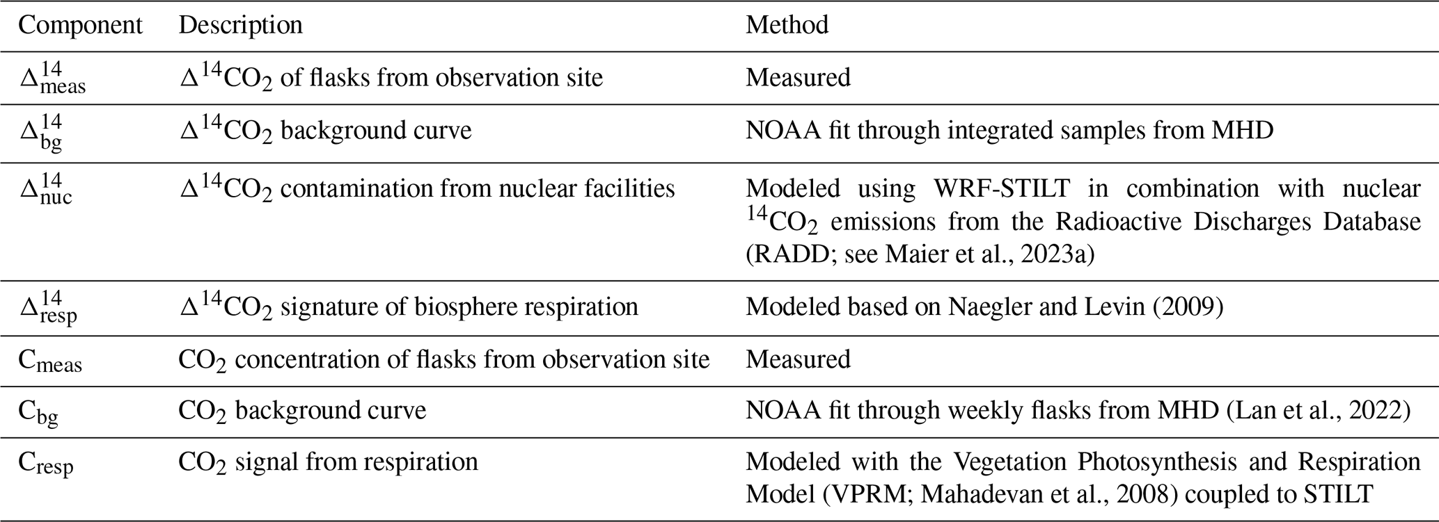
To calculate the ¹⁴C-based < ΔCO $/$ ΔffCO₂ > ratio from flasks, we first estimate the ΔffCO₂ concentrations from the Δ¹⁴CO₂ difference between the Heidelberg and OPE measurements and smoothed fits through the MHD background data. For this, we use the following Eq. (2) from Maier et al. (2023a), which also contains a correction for contaminating ¹⁴CO₂ emissions from nuclear facilities and for the potentially ¹⁴C-enriched Δ¹⁴CO₂ signature of biosphere respiration (still releasing stored nuclear bomb ¹⁴CO₂ to the atmosphere):

$$\begin{array}{}\text{(2)}& \begin{array}{rl}\mathrm{\Delta }{\mathrm{ffCO}}_{\mathrm{2}}& ={\mathrm{C}}_{\mathrm{bg}}\cdot {\displaystyle \frac{{\mathrm{\Delta }}_{\mathrm{bg}}^{\mathrm{14}}-{\mathrm{\Delta }}_{\mathrm{meas}}^{\mathrm{14}}}{{\mathrm{\Delta }}_{\mathrm{meas}}^{\mathrm{14}}+\mathrm{1000}\mathrm{‰}}}\\ & +{\mathrm{C}}_{\mathrm{meas}}\cdot {\displaystyle \frac{{\mathrm{\Delta }}_{\mathrm{nuc}}^{\mathrm{14}}}{{\mathrm{\Delta }}_{\mathrm{meas}}^{\mathrm{14}}+\mathrm{1000}\mathrm{‰}}}\\ & +{\mathrm{C}}_{\mathrm{resp}}\cdot {\displaystyle \frac{{\mathrm{\Delta }}_{\mathrm{resp}}^{\mathrm{14}}-{\mathrm{\Delta }}_{\mathrm{meas}}^{\mathrm{14}}}{{\mathrm{\Delta }}_{\mathrm{meas}}^{\mathrm{14}}+\mathrm{1000}\mathrm{‰}}}.\end{array}\end{array}$$

Table 1 shows a compilation of all components of Eq. (2) with short explanations. In general, we used the same procedure as described by Maier et al. (2023a) to estimate the correction terms in Eq. (2). Note that we only use the flask results with a modeled nuclear contamination below 2 ‰, to avoid nuclear corrections whose uncertainty exceeds the typical uncertainty in the Δ¹⁴CO₂ measurements (see Maier et al., 2023a).

Table 1 Description of the components in Eq. (2).

We then use the weighted total least-squares algorithm from Wurm (2022) to calculate regression lines to the ΔCO and ¹⁴C-based ΔffCO₂ concentrations of the 343 flasks from Heidelberg and the 52 flasks from OPE. This regression algorithm is built on the code from Krystek and Anton (2007) and considers uncertainties in both the ΔCO and ΔffCO₂ flask concentrations. In this study, we force the regression line through the origin. Thus, we assume that the very well-mixed and clean air masses at the observation sites without ΔffCO₂ excess also represent the background CO concentrations at MHD. The slope of the regression line then gives an estimate of the < ΔCO $/$ ΔffCO₂ > ratio for the corresponding observation site and time period of the flask samples. In Appendix A1, we show why one should use a regression algorithm which considers the uncertainties in the dependent and independent variables, to calculate a mean bias-free < ΔCO $/$ ΔffCO₂ > ratio instead of error-weighted means or median estimates from individual samples.

2.2.2 Modeling of inventory-based ΔCO $/$ ΔffCO₂ ratios

To compare the ¹⁴C-based ΔCO $/$ ΔffCO₂ ratios with inventory-based ratios, we need to weigh the bottom-up emissions with the footprints of the observation sites. For this, we use the following modeling setup to simulate hourly ΔCO and ΔffCO₂ excess at the Heidelberg and OPE observation sites. The Stochastic Time-Inverted Lagrangian Transport (STILT) model (Lin et al., 2003) is coupled with the Weather Research and Forecasting (WRF) model (Nehrkorn et al., 2010), which is driven by the high-resolution CO and ffCO₂ emission fluxes from the TNO inventories (Dellaert et al., 2019; Denier van der Gon et al., 2019). The WRF-STILT domain expands from 37 to 61° N and from 10° W to 23° E (see Fig. 1). The input meteorological fields are taken from the European Reanalysis v5 data from the European Centre for Medium-Range Weather Forecasts (ECMWF) with a horizontal resolution of 0.25° (Hersbach et al., 2020). The WRF model setup combines an inner domain with a 2 km horizontal resolution along the Rhine Valley (red rectangle in Fig. 1) nested in a larger European domain with a 10 km resolution used to calculate the hourly footprints with STILT. Those footprints are then mapped with the high-resolution CO and ffCO₂ emissions from TNO to get the CO and ffCO₂ concentrations for Heidelberg and OPE. As we assume zero CO and ffCO₂ concentrations at the boundaries of the STILT model domain, the modeled CO and ffCO₂ concentrations directly correspond to the ΔCO and ΔffCO₂ excesses with respect to the model domain boundaries. The TNO inventory divides the total CO and ffCO₂ emissions into 15 emission sectors with individual monthly, weekly, and diurnal temporal emission profiles. Note that the CO emissions from TNO contain the fossil fuel and biofuel CO contributions. This also includes emissions from the agricultural sector, like agricultural waste burning. However, in this study, we fully neglect natural CO sources, like emissions from forest fires, and CO sinks and atmospheric CO chemistry. The TNO inventory also distinguishes between point source and area source emissions. As Heidelberg is surrounded by many point sources with elevated stacks, we treat the TNO point sources within the Rhine Valley separately with the STILT volume source influence (VSI) approach (see Maier et al., 2022), to model the point source contributions at the Heidelberg site.

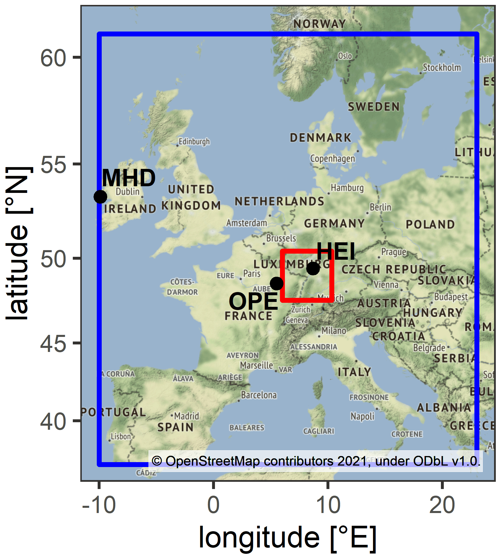
Figure 1 Map of the European WRF-STILT model domain (framed in blue). The Heidelberg (HEI) and OPE observation sites as well as the Mace Head (MHD) background site are indicated. The red rectangle shows the Rhine Valley domain.

3 Results

3.1 Study at the urban site Heidelberg

3.1.1 ¹⁴C-based ΔCO $/$ ΔffCO₂ ratios from flask samples

Figure 2 shows the ¹⁴C-based ΔCO $/$ ΔffCO₂ ratios of the hourly flask samples from Heidelberg, which were collected under very different atmospheric conditions (see colors in Fig. 2). By testing different flask sampling strategies, we sampled very different situations from almost background conditions, nighttime CO₂ enhancements, morning and evening rush-hour signals, and local contaminations to large-scale synoptic events and diurnal patterns. We observe large positive ratios as well as negative ratios with enormous error bars, mainly during summer and under well-mixed atmospheric (background) conditions (green dots). These outliers are associated with very low (or even negative) ΔffCO₂ concentrations and large relative ΔffCO₂ uncertainties that inflate the ratio and its uncertainty. Indeed, these individual unrealistic ratios can lead to a bias in the mean or median of the (averaged) ratios, as we show with a synthetic-data study in Appendix A1. However, the slope of an error-weighted regression through the flask ΔCO and ΔffCO₂ excess concentrations represents an unbiased estimate of the < ΔCO $/$ ΔffCO₂ > ratio (see Fig. 3a).

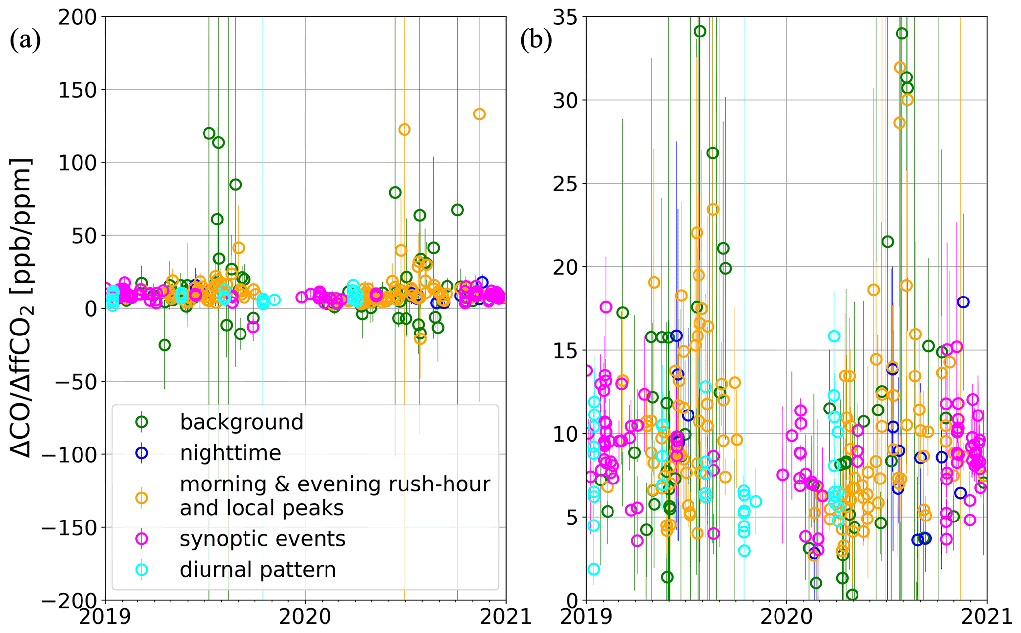
Figure 2 ¹⁴C-based ΔCO $/$ ΔffCO₂ ratios from hourly flasks collected at the Heidelberg observation site between 2019 and 2020. Very different atmospheric conditions are sampled, as indicated by the different colors. We sampled almost background conditions (green), CO₂ enhancements during the night (blue), morning and evening rush-hour peaks and CO₂ spikes (most probably from local sources; orange), synoptic events with a CO₂ concentration built up over several days (magenta), and diurnal cycles (cyan). Panel (b) shows a zoom into panel (a).

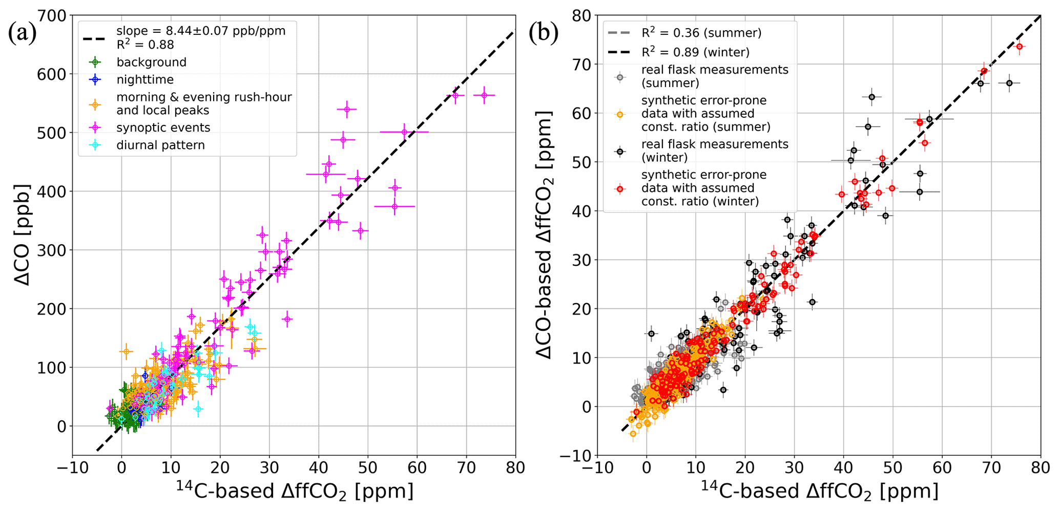
Figure 3 (a) Scatterplot with the measured ΔCO and the ¹⁴C-based ΔffCO₂ concentrations of the hourly flasks collected at the Heidelberg observation site between 2019 and 2020. The colors indicate the sampling situation of the flasks (see description in the caption of Fig. 2). The black dashed line shows a regression line calculated with the weighted total least-squares algorithm from Wurm (2022). (b) Comparison between the ΔCO-based ΔffCO₂ (from Eq. 1) and the ¹⁴C-based ΔffCO₂ concentrations of the Heidelberg winter (black dots) and summer (gray dots) flasks. The red (winter data) and orange (summer data) dots show the synthetic ΔCO-based ΔffCO₂ estimates and the synthetic error-prone ΔffCO₂ concentrations, which cover the same range as the ¹⁴C-based ΔffCO₂ observations. The synthetic ΔCO-based ΔffCO₂ data were generated by assuming a constant ΔCO $/$ ΔffCO₂ ratio, which is the average < ΔCO $/$ ΔffCO₂ > ratio from the Heidelberg flasks. Therefore, the scattering of the orange and red data points is only caused by the measurement and background representativeness uncertainties in the ΔCO and ¹⁴C-based ΔffCO₂ concentrations. This means that the increased scattering of the real data (black and gray) compared with the synthetic data (red and orange) is caused by the variability in the ratios. A more detailed description of how the synthetic data were generated can be found in the text (Sect. 3.1.2 and Appendix A1).

The slope of this regression yields an average ratio of 8.44 ± 0.07 ppb ppm⁻¹ for all flasks collected during the 2 years (2019 and 2020). The good correlation indicated by an R² value of 0.88 is predominantly caused by the flasks with large ΔCO and ΔffCO₂ concentrations, which were mainly collected during synoptic events in the winter half-year (see Fig. A2). While limiting the analysis to the cold-season flasks gives a ratio of 8.52 ± 0.08 ppb ppm⁻¹ with a high correlation (R²=0.89), the warm-season flasks are associated with a slightly smaller ratio of 8.08 ± 0.17 ppb ppm⁻¹ but a much poorer correlation (R²=0.36). Thus, there might be a seasonal cycle in the relationships between ΔCO and ΔffCO₂, with the correlation being strong in the cold period but much weaker during the warm period. However, there is no evidence of a significant seasonal cycle in the ratios, with the winter ratio being only 5 % larger than the summer ratio. Therefore, the seasonal cycle is not in the ratio itself but, rather, more in its significance or robustness. The daily cycle of the ratios also seems to be small. The afternoon flasks show an average ratio of 8.60 ± 0.19 ppb ppm⁻¹ (R²=0.84), while non-afternoon flasks show an average ratio of 8.41 ± 0.08 ppb ppm⁻¹ (R²=0.88). Furthermore, there is only a slightly decreasing trend between 2019 (8.57 ± 0.11 ppb ppm⁻¹, R²=0.87) and the COVID-19 year of 2020 (8.35 ± 0.10 ppb ppm⁻¹, R²=0.88), although this is within the 2σ uncertainty range.

3.1.2 Uncertainty in the ΔCO-based ΔffCO₂ record

Because of the small daily and seasonal differences in the ¹⁴C-based ΔCO $/$ ΔffCO₂ ratios and the difficulty with respect to calculating average summer ratios due to decreased correlation (see Appendix A1), we decided to use the average ratio of all flasks to compute a continuous hourly ΔCO-based ΔffCO₂ record for the 2 years (2019 and 2020). However, this means that we fully neglect any spatiotemporal variability in the ratios. At times when we have collected flasks, we can then compare these ΔCO-based ΔffCO₂ estimates with the ¹⁴C-based ΔffCO₂ concentrations of the flasks (see the black dots in Fig. 3b). Obviously, a regression through these data yields a slope of 1, as we used the average ratio of all flasks to construct the ΔCO-based ΔffCO₂ record. The (vertical) scattering of the data around this 1:1 line, e.g., the root-mean-square deviation (RMSD) between ΔCO- and ¹⁴C-based ΔffCO₂, can be used as an estimate of the uncertainty in the ΔCO-based ΔffCO₂ record. This RMSD is 3.95 ppm, which is almost 4 times larger than the typical uncertainty for ¹⁴C-based ΔffCO₂. As the RMSD depends on the range of the ΔffCO₂ concentrations, we also compute a normalized RMSD (NRMSD), by dividing the RMSD by the mean ¹⁴C-based ΔffCO₂ concentration of the flasks. This gives an NRMSD of 0.39, which means that the RMSD equals 39 % of the average ΔffCO₂ excess at Heidelberg.

In the following, we want to establish the sources of this increased uncertainty. Thus, we assess if it is mainly caused by the measurement and background representativeness uncertainties in the ΔCO and ¹⁴C-based ΔffCO₂ concentrations or if it is rather due to the variability in the ratios that we fully neglect when using a constant ratio to derive the ΔCO-based ΔffCO₂ record. To answer this, we performed a synthetic-data experiment, in which we assumed a “true” constant ΔCO $/$ ΔffCO₂ ratio of 8.44 ppb ppm⁻¹. We used this constant ratio and the observed ¹⁴C-based ΔffCO₂ concentrations from the flasks to create synthetic “true”, i.e., error-free, ΔCO and ΔffCO₂ data pairs (see Appendix A1). We then drew random numbers from an unbiased Gaussian distribution with a 1σ range of 1.16 ppm (for ΔffCO₂) and 14.49 ppb (for ΔCO), which represents the mean ΔCO and ΔffCO₂ uncertainties in the real measurements (see Sect. 2.2). These random numbers were added to the synthetic “true” ΔCO and ΔffCO₂ data to get error-prone synthetic ΔCO and ΔffCO₂ concentrations. After that, we used the error-prone synthetic ΔCO data and the ΔCO $/$ ΔffCO₂ ratio of 8.44 ppb ppm⁻¹ to calculate synthetic ΔCO-based ΔffCO₂ concentrations. By comparing the error-prone synthetic ΔffCO₂ concentrations with the synthetic ΔCO-based ΔffCO₂ concentrations, we get a lower RMSD of only 2.07 ppm. By construction, this synthetic-data experiment covers the same ΔCO and ΔffCO₂ ranges as the real flask observations but assumes a constant ratio. Therefore, the difference between the RMSD of the real ΔffCO₂ observations (3.95 ppm) and the synthetic data (2.07 ppm) must be caused by the variability in the ratios. Thus, about half of the uncertainty in the ΔCO-based ΔffCO₂ record can be attributed to uncertainties in the ΔCO and ΔffCO₂ excess concentrations, whereas the remaining half of this uncertainty originates from the variability in the ratios.

3.1.3 Comparison of observed and inventory-based ΔCO $/$ ΔffCO₂ ratios

We also compared our flask ¹⁴C-based ΔCO $/$ ΔffCO₂ ratios with the high-resolution emission inventory from TNO. We simulated the hourly ΔCO and ΔffCO₂ contributions in Heidelberg, by transporting the CO and ffCO₂ emissions from the TNO inventory over the European STILT domain (see Fig. 1). Figure 4a shows, for the flask sampling events in 2019 and 2020, the respective simulated ΔCO and ΔffCO₂ results (red and blue dots). In contrast to the flask observations (gray crosses), the simulated data do not scatter around a single regression line corresponding to a constant ratio. The model results rather show two branches indicating two different ratios. If the contributions from point sources in the simulated ΔffCO₂ are larger than 50 % (red points in Fig. 4a), the data scatter around a regression line with a slope of 2.04 ± 0.23 ppb ppm⁻¹ and a poor correlation ($R^{\mathrm{2}}=-\mathrm{0.05}$). However, if the contributions from point sources in the simulated ΔffCO₂ are below 50 % (blue points in Fig. 4a), the data yield a ratio of 5.21 ± 0.06 ppb ppm⁻¹ with a good correlation (R²=0.91).

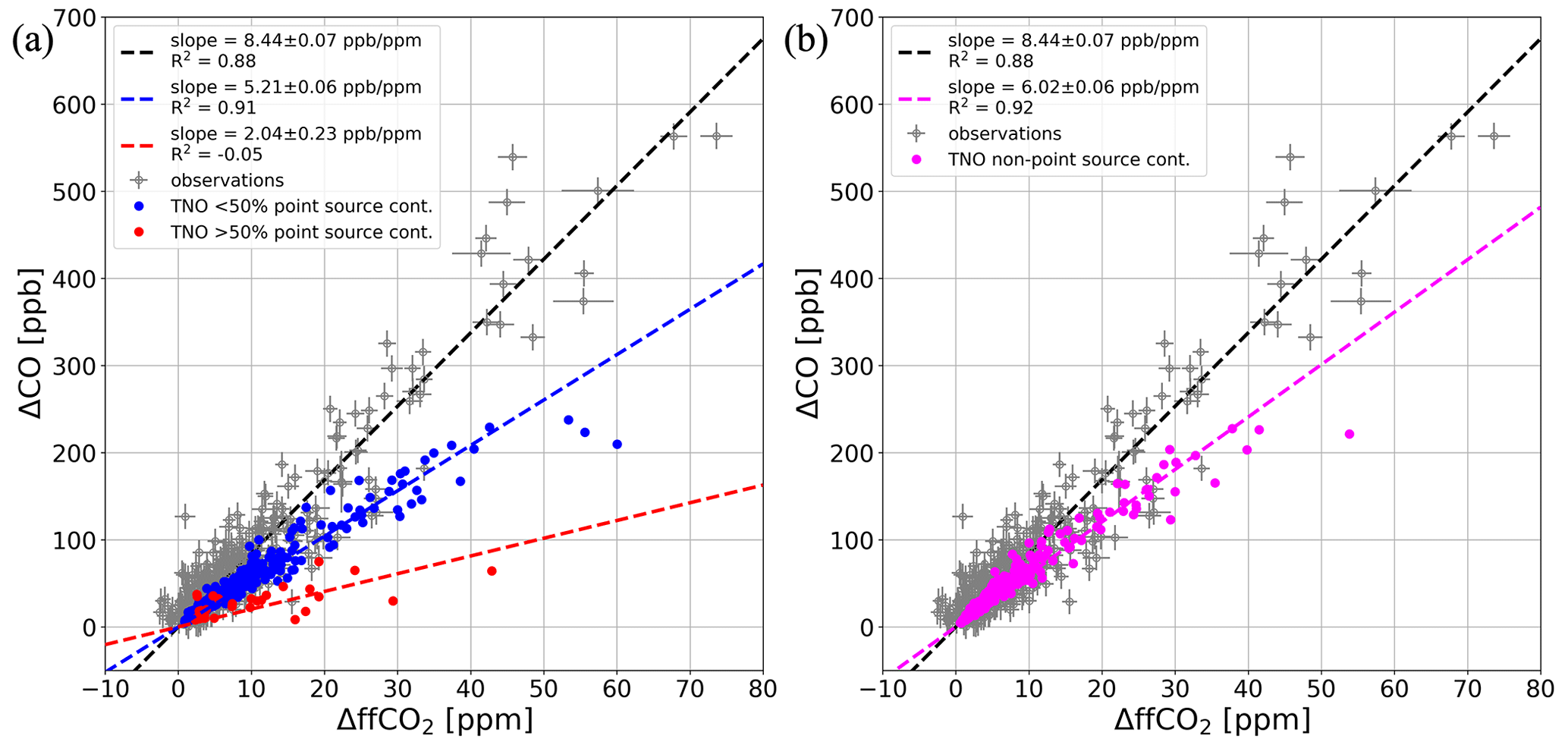
Figure 4 WRF-STILT simulation of the TNO ΔCO and ΔffCO₂ contributions in Heidelberg, 30 m, from emissions within the European STILT domain (see Fig. 1). The model results are shown only for hours with flask sampling events between 2019 and 2020. The blue and red points in panel (a) indicate hourly situations with a point source contribution of less and more than 50 %, respectively. The magenta dots in panel (b) show the non-point-source contributions only. As a reference, the flask observations are also shown in gray. The dashed lines show linear regressions through the respective data points.

This comparison with the flask observations highlights two complementary findings. First, the Heidelberg observation site is rarely influenced by events with strong point source contributions larger than 50 % because hardly any of the observed ratio scatters around the red regression line in Fig. 4a and thus shows a point-source-dominated ratio (that lies around 2 ppb ppm⁻¹). Hence, the model results for Heidelberg often overestimate the contributions from point sources. Second, the area-source-dominated model results with point source contributions smaller than 50 % show an equally high correlation compared to the observations. This indicates that the emission ratios for the dominating heating and traffic sectors are probably currently quite similar in the main footprint of Heidelberg. However, the 5.2 ppb ppm⁻¹ ratio found in the model results is almost 40 % lower compared with the 8.44 ppb ppm⁻¹ observed ratio. The magenta dots in Fig. 4b show the modeled ΔCO and ΔffCO₂ contributions from the non-point-source emissions alone. They lead to an average ratio of 6.02 ± 0.06 ppb ppm⁻¹ (R²=0.92). This might indicate that TNO underestimates the ratios of the area source emissions in the Rhine Valley. This finding is striking because it means that inventory-based ratios would lead to large biases if they were used to calculate a ΔCO-based ΔffCO₂ record for Heidelberg. It underlines the added value of the station-based observations and the necessary support for long-term monitoring. In the following, we present the results of our study performed at the rural ICOS site OPE.

3.2 Study at the rural ICOS site OPE

We now want to investigate if the flask observations from a more remote site can be used for estimating a continuous ΔCO-based ΔffCO₂ record. Figure 5a shows the ΔCO and ¹⁴C-based ΔffCO₂ observations of 52 flasks from the OPE station, which were collected nearly every third day between September 2020 and March 2021 in the early afternoon. The flasks have an average ΔffCO₂ concentration of 2.19 ppm showing that OPE is much less influenced by polluted air masses compared with the urban site Heidelberg. The regression algorithm from Wurm (2022) gives an average flask ΔCO $/$ ΔffCO₂ ratio of 11.49 ± 0.81 ppb ppm⁻¹ (R²=0.70), which is 3 ppb ppm⁻¹ larger than the average ratio observed in Heidelberg during 2019 and 2020. Furthermore, the 1σ uncertainty in the slope of the regression line is 10 times larger compared with Heidelberg. This comes along with a reduced correlation between ΔCO and ΔffCO₂ and can at least partly be explained by the smaller range of ΔffCO₂ concentrations sampled at OPE (see Appendix A1). As all flasks were collected in the winter half-year and during the afternoon, it is not possible to draw conclusions about potential seasonal or diurnal cycles in the ΔCO $/$ ΔffCO₂ ratios at OPE.

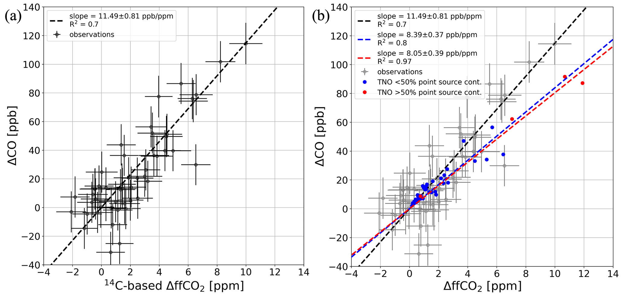
Figure 5 (a) ΔCO and ΔffCO₂ concentrations from hourly afternoon flasks collected at the OPE station between September 2020 and March 2021. The black dashed line shows a regression line performed with the weighted total least-squares algorithm from Wurm (2022). (b) WRF-STILT simulation of the TNO ΔCO and ΔffCO₂ contributions at OPE from emissions within the European STILT domain (see Fig. 1) for the hours with flask sampling events at OPE. The blue and red points indicate hourly situations with a point source contribution of less and more than 50 %, respectively. As a reference, the flask observations are also shown in gray. The dashed lines show linear regressions through the respective data points.

Again, we want to use this estimated ratio from the collected flasks to calculate, with Eq. (1), an hourly ΔCO-based ΔffCO₂ record for OPE. The RMSD between the ΔCO-based ΔffCO₂ and the ¹⁴C-based ΔffCO₂ from the flasks is only 1.49 ppm, which is due to the much smaller ΔffCO₂ excess at OPE compared with Heidelberg. However, the NRMSD is 0.68, which indicates that the RMSD is almost 70 % of the average ΔffCO₂ afternoon signal at OPE during September 2020 and March 2021. We perform a similar synthetic-data experiment to that carried out for Heidelberg (see Sect. 3.1.2) to investigate which share of the RMSD can be attributed to the uncertainty in the observations and which part is due to the (neglected) spatiotemporal variability in the ratios. The comparison of the synthetic ΔCO-based and ¹⁴C-based ΔffCO₂ data leads to an RMSD of 1.61 ± 0.16 ppm, which already exceeds the observed RMSD of 1.49 ppm between the observed ΔCO and ¹⁴C-based ΔffCO₂. Thus, the ΔCO and ¹⁴C-based ΔffCO₂ uncertainties can fully explain the observed RMSD, and the spatiotemporal variability in the ratios in the footprint of the OPE site seems to have only a secondary influence.

Finally, Fig. 5b shows the simulated ΔCO and ΔffCO₂ contributions for the flask sampling hours at OPE. A linear regression through the data yields an average ratio of 8.18 ± 0.24 ppb ppm⁻¹ with high correlation (R²=0.93). There is only a very small difference < 5 % between the average ratio of the situations with point source contributions lower than 50 % (blue points) and the very few events with point source contributions larger than 50 % (red points). This indicates that the simulations do not show events with purely point-source-dominated contributions at OPE, which is in agreement with the observations. However, the ratio estimated from the model results is 29 % lower than the ratio from the observations. In contrast, the area source emissions alone would lead to an average ratio of 10.98 ± 0.53 ppb ppm⁻¹, which is well within the uncertainty range of the observed ratio. This could indicate that the contributions from point sources are still overestimated by STILT and/or that the emission ratio of the area sources in the footprint of the OPE site are underestimated by TNO. Furthermore, there might be additional non-fossil CO sources in the footprint of the station, such as biomass burning, which were ignored in STILT.

4 Discussion

4.1 How large is the uncertainty in an hourly ΔCO-based ΔffCO₂ estimation based on ¹⁴C flask observations?

Vogel et al. (2010) estimated ΔCO-based ΔffCO₂ at the Heidelberg observation site, using ΔCO $/$ ΔffCO₂ ratios from weekly integrated ¹⁴CO₂ samples. As the weekly ratios are weighted by the ΔffCO₂ excess, the ΔCO-based ΔffCO₂ estimation is biased towards hours with high ΔffCO₂. Therefore, Vogel et al. (2010) used flasks to sample the diurnal cycles in summer and winter, in order to correct the weekly averaged ratios with the diurnal variations. This diurnal cycle correction allowed them to reduce some of the bias in the ΔCO-based ΔffCO₂ estimates. In the present study, we follow up their estimation based on weekly integrated samples using recently collected hourly flask samples. Our aim is to investigate whether flask samples collected with higher frequency and higher temporal resolution can be used to estimate a continuous ΔCO-based ΔffCO₂ record and assess the related uncertainty. We used results from hourly flask samples at two contrasting sites, the urban Heidelberg and the rural OPE stations.

4.1.1 Results from the urban site Heidelberg

In Heidelberg, almost 350 ¹⁴CO₂ flask samples were collected during very different situations between 2019 and 2020. Their ΔCO and ΔffCO₂ excess concentrations compared to the marine background from MHD show a strong correlation, with an R² value of 0.88 (see Fig. 3a). This indicates that the emission ratios of the traffic and heating sectors, which dominate the urban emissions, are quite similar in the main footprint of Heidelberg and the investigated period of time. Furthermore, it follows that the Heidelberg observation site with an air intake height of 30 m above the ground is hardly influenced by plumes from nearby point sources, which are associated with rather low emission ratios because large combustion units like power plants have a high combustion efficiency (Dellaert et al., 2019). Indeed, there are very small differences (below 3 %) between the mean afternoon and non-afternoon ratios and between the average ratios in 2019 and 2020. Moreover, there is almost no seasonal cycle in the ratios, as the average ratio of the flasks collected in the summer half-year is ca. 5 % smaller than the average ratio of the flasks from the winter half-year. However, there is a seasonal cycle in the ratios' robustness, as underlined by the contrasting R² values between winter and summer.

Thus, we must emphasize the difficulty involved in estimating reliable ratios for the summer period and even question the meaning of such an approach. If, for example, only the flasks from the three main summer months, June, July, and August, are considered, the correlation between ΔCO and ΔffCO₂ disappears (R²=0.06), which prohibits the calculation of average summer ratios (see Appendix A1). This has also been found by other studies (Vogel et al., 2010; Miller et al., 2012; Turnbull et al., 2015; Wenger et al., 2019) and can be explained by smaller ΔffCO₂ signals, e.g., due to higher mixing volumes in summer, with large relative uncertainties (see Appendix A1) and/or by the increased contribution from non-fossil CO sources during summer (Vimont et al., 2019). Nevertheless, we estimated the average ratio from summer and winter flasks and neglected a potential seasonal cycle in the ratios. However, the global regression line fitting is mostly dominated by the flasks with large ΔCO and ΔffCO₂ concentrations, which were predominantly collected during synoptic events in the winter half-year.

The comparison of the ΔCO-based ΔffCO₂ estimates with the ¹⁴C-based ΔffCO₂ data from the flasks gives an RMSD of about 4 ppm, which we use as an estimate for the 1σ uncertainty of the ¹⁴C-calibrated ΔCO-based ΔffCO₂ concentrations. One-half of this uncertainty could be attributed to the measurement uncertainty and the representativeness uncertainty of the CO and Δ¹⁴CO₂ background from the marine site MHD. The other half of this uncertainty is related to the ratio variability in the main footprint of Heidelberg, which has been ignored by applying a constant ratio to calculate the ΔCO-based ΔffCO₂ concentrations. Overall, this uncertainty is almost 4 times larger than the typical uncertainty of ¹⁴C-based ΔffCO₂ estimates and corresponds to ca. 40 % of the mean ΔffCO₂ signal of the flasks collected in Heidelberg. However, by using the average ratio from the flasks, we got an almost bias-free ΔCO-based ΔffCO₂ record with an hourly resolution. In the companion paper (Maier et al., 2024), we demonstrate that this continuous ΔCO-based ΔffCO₂ record, although with a 4-fold larger uncertainty, currently provides more valuable information about the ffCO₂ emissions in the urban region around Heidelberg than the discrete (and sparser) ¹⁴C-based ΔffCO₂ estimates with a small uncertainty. Of course, if the ¹⁴C-based ΔffCO₂ had a similar temporal resolution to the ΔCO-based ΔffCO₂, the information content of the ¹⁴C-based ΔffCO₂ would be higher than that of the ΔCO-based ΔffCO₂. However, as this is not (yet) the case, we conclude that the usage of ΔCO-based ΔffCO₂ to infer ffCO₂ emissions could be a valuable approach for other urban sites.

4.1.2 Results from the rural site OPE

At OPE, afternoon ¹⁴C flasks were collected nearly every third day between September 2020 and March 2021. As this does not cover a full year, it is not possible to investigate the potential diurnal or seasonal cycle in the ratios. As in the case of Heidelberg, a constant ratio was used to compute the ΔCO-based ΔffCO₂ record. The flask ΔCO and ¹⁴C-based ΔffCO₂ excess show a lower correlation (R²=0.7) than the flasks from the urban site Heidelberg (R²=0.88). This might be explained by the almost 80 % lower mean signal of the flasks collected at OPE and the smaller number of flask samples. This affects the uncertainty of the slope of the regression line, which is 0.81 ppb ppm⁻¹ at OPE – more than 10 times larger than that in Heidelberg. The RMSD between the ΔCO-based ΔffCO₂ and the ¹⁴C-based ΔffCO₂ from the flasks is 1.5 ppm, which accounts for almost 70 % of the mean ΔffCO₂ signal from the flasks. This RMSD is only about 30 % higher than the typical ¹⁴C-based ΔffCO₂ uncertainty. This could be explained by the fact that we only considered the cold period at OPE and that this rural site might be less influenced by the ratio variability. We determined that the whole RMSD of 1.5 ppm can entirely be explained by the measurement uncertainties and the representativeness uncertainty of the background concentrations. Such low ratio variability is expected at more remote sites like OPE, as air masses have a long-range transport history with mixing and smoothing of various surface sources. Therefore, this ΔCO-based ΔffCO₂ record with continuous data coverage, if well calibrated with ¹⁴CO₂ measurements, could be a valuable addition to discrete ¹⁴C-based ΔffCO₂ estimates for constraining ffCO₂ emissions for afternoon situations during the winter period.

4.2 How many ¹⁴CO₂ flask measurements are needed to estimate a reliable continuous ΔCO-based ΔffCO₂ record?

We use the STILT forward runs to assess the representativeness of the collected flask samples for the entire period covered by the ΔCO-based ΔffCO₂ record. We compute the average STILT ΔCO $/$ ΔffCO₂ ratios by fitting a regression line through the simulated ΔCO and ΔffCO₂ data for (1) the hours with flask samples only and for (2) all hours covered by the ΔCO-based ΔffCO₂ record. As the STILT results suggest an unrealistic simulation of situations with more than 50 % point source influence in Heidelberg, we restricted the analysis to the hours during which STILT predicts a point source influence below 50 %. Note that this is by far the largest pool of data (see Fig. 4a). For Heidelberg, this comparison gives a difference smaller than 3 % between the average modeled ratio of the hours with flask sampling events and the average modeled ratio of all hours between 2019 and 2020. This result suggests that the Heidelberg flasks are quite representative for these 2 years. In the case of OPE, the STILT average ratio of the hours with flask samples differs by less than 1 % from the average ratio of all afternoon hours between September 2020 and March 2021, again indicating that the flask samples are very representative of the afternoons during this period. Interestingly, STILT suggests a small diurnal cycle in the OPE ratios, with an 8 % difference between the mean ratios of the afternoon and the non-afternoon hours, respectively.

After having shown that the flask pools from both observation sites seem to be quite representative, we investigate how many flasks are needed to determine a robust average ratio to construct the ΔCO-based ΔffCO₂ record. For this, we perform a small bootstrapping experiment. We randomly select i flasks from the Heidelberg (and OPE) flask pool, with i ranging from 3 to the total number of flasks N_tot (N_tot=343 flasks in Heidelberg and N_tot=52 flasks at OPE). Then, we calculate an average ratio < R_i,j > from the ΔCO and ΔffCO₂ data of the i flasks using the regression algorithm from Wurm (2022). We repeat this experiment j=100 times for each i. After that, we can calculate the standard deviation σ(< R_i >) over the 100 realizations of {< R_i,1 >, …, < R_i,100 >} for each i. Obviously, for i=N_tot, we get the average flask ratio < R_flask > and σ(< $R_{i=N_{\mathrm{tot}}}$ >) = 0, as we used all available flasks. Figure 6 shows the relative standard deviation (σ(< R_i >) $/$ < R_flask >) for different shares ($i/N_{\mathrm{tot}}$) of flasks used to calculate the ratio. Apparently, this relative standard deviation of the ratio increases with a decrease in the number of flasks used to calculate the ratio. At the urban site Heidelberg, we would need 15 flasks, (i.e., less than 5 % of our flask pool) to keep the standard deviation of the ratio below 10 %. At the more remote site OPE, we would need 20 flasks (i.e., almost 40 % of the collected OPE flasks) to reduce the standard deviation of the ratio to 10 %.

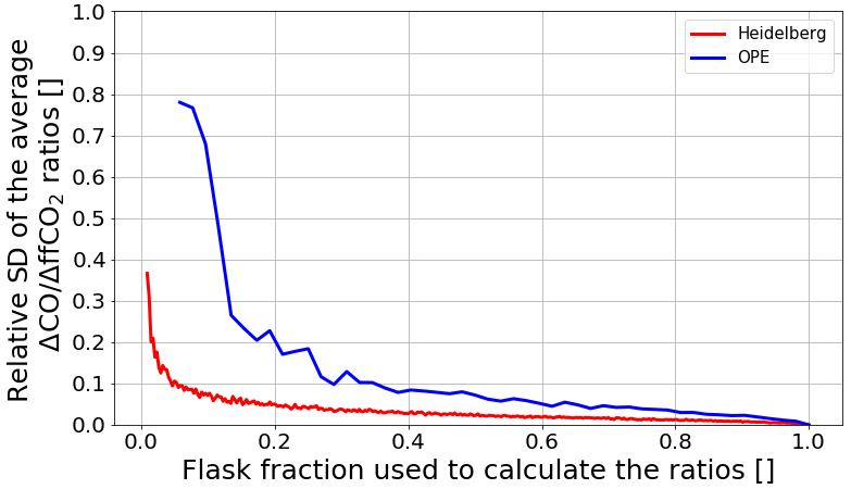
Figure 6 Results of the bootstrapping experiment. We used an increasing number of random flasks from the Heidelberg (in red) and OPE (in blue) flask pools to deduce an average ΔCO $/$ ΔffCO₂ ratio. For each number of flasks, we repeat this experiment 100 times. Finally, we calculate the standard deviation of the average ratios over the 100 repetitions for each number of flasks. Here, we show the relative standard deviation (SD) of the average ratios for an increasing flask fraction used to calculate the ratios. A flask fraction of 1 means that all available flask samples from Heidelberg and OPE, respectively, were used to calculate the average ratios. Obviously, this leads to a standard deviation of 0. The reader is referred to the text for a detailed description of the bootstrapping experiment.

Overall, this experiment shows that the number of flasks needed to determine a robust average ΔCO $/$ ΔffCO₂ ratio with an uncertainty below 10 % depends on the correlation between the ΔCO and ΔffCO₂ data. For R² values between 0.7 and 0.9, it takes about 15 to 20 flasks to determine the average ΔCO $/$ ΔffCO₂ ratio with an uncertainty of less than 10 %. However, these flasks must cover a wide range of the observed ΔCO and ΔffCO₂ concentrations. As mentioned above, the determination of an average ratio is associated with much larger uncertainties during summer, with typically lower R² values. Thus, in order to investigate a potential seasonal cycle in the ratios, it is important to also collect flasks during summer situations with large ΔCO concentrations. This might increase the chance of getting better correlations and, thus, lower uncertainties in the summer ratios. As we considered only one urban and one rural station in this study, we recommend repeating this experiment at further sites to confirm general applicability.

4.3 Can inventory-based ΔCO $/$ ΔffCO₂ ratios be used to construct the ΔCO-based ΔffCO₂ record?

Flask-based ΔCO $/$ ΔffCO₂ ratios are independent station-based estimations not influenced by sector-specific inventory emission factors and transport model uncertainties. Moreover, they intrinsically include all potential CO contributions from natural and anthropogenic sources and sinks. However, for many observation sites with continuous CO measurements but without ¹⁴C measurements, the use of inventory-based ΔCO $/$ ΔffCO₂ ratios is the only option to estimate hourly ΔCO-based ΔffCO₂ estimates. Therefore, we also compared the flask-based ratios from Heidelberg and OPE with ΔCO $/$ ΔffCO₂ ratios from the TNO inventory transported with STILT to those observational stations.

At the urban site Heidelberg, the model-based estimations face two issues. First, the model predicts events with pure point source emissions which have very low ΔCO $/$ ΔffCO₂ ratios of about 2 ppb ppm⁻¹ but are hardly observed at the observation site. This illustrates the deficits of STILT with respect to correctly simulating the contributions from point source emissions. Thus, even the improved STILT-VSI approach, which considers the effective emission heights of the point sources seems to overestimate the contributions from point sources for individual hours. Second, the contributions from the non-point-source emissions alone would lead to an average ratio that is almost 30 % lower than the average flask ratio (see Fig. 4b). This might indicate that the TNO area source emission ratios are too low in the main footprint of Heidelberg. We further investigated the traffic and heating sectors separately, which are together responsible for the main share of the non-point-source emissions in the Rhine Valley. Figure A3 shows the ΔCO and ΔffCO₂ contributions from the traffic (orange dots) and heating sector (cyan dots). The traffic (biofuel plus fossil fuel) sector leads to an average ΔCO $/$ ΔffCO₂ ratio of 7.72 ± 0.08 ppb ppm⁻¹ (R²=0.93), which is less than 10 % lower than the observed average ratio of 8.44 ± 0.07 ppb ppm⁻¹. However, the heating (wood plus fossil fuel) sector leads to a much lower average ratio of 3.36 ± 0.09 ppb ppm⁻¹ (R²=0.65). If the TNO area source emissions are indeed too low in the main footprint of Heidelberg, this could be explained by the TNO heating sector and, for example, by an incorrect distribution of the use of fossil fuels and biofuels in the heating sector. Moreover, the differences between the TNO emission ratios of the traffic and heating sectors lead to a seasonal cycle in the modeled (area source) ΔCO $/$ ΔffCO₂ ratios during the flask sampling times, with an almost 20 % lower average ratio in the winter half-year compared with the summer half-year. Such a strong seasonal cycle is not shown by the flask observations (see Fig. A2).

Indeed, the emission ratios of the heating sector come along with large uncertainties. In particular, the share of wood combustion has a major impact on the ΔCO $/$ ΔffCO₂ ratios of the total heating sector, as it releases no ffCO₂ emissions but substantial CO emissions. In TNO, the proximity to forested areas (access to wood) is used as a proxy to determine the share of wood combustion within a grid cell (Kuenen et al., 2022). During two measurement campaigns in two villages around Heidelberg, Rosendahl (2022) showed that this can cause huge biases between the measured and inventory-based heating ratios. From local measurements in the urban village of Leimen, a few kilometers south of Heidelberg, Rosendahl (2022) estimated an average heating ratio of 8.02 ± 3.12 ppb ppm⁻¹ for 2 weeks in March 2021, whereas TNO predicted an average heating ratio of 1.79 ppb ppm⁻¹. This discrepancy is of a similar magnitude to that in our study. However, Rosendahl (2022) showed that the measurements agreed better with the TNO inventory in a more rural village near Heidelberg. Overall, it seems that the TNO emission inventory underestimates the ΔCO $/$ ΔffCO₂ ratios in the main footprint of Heidelberg during the 2 study years (2019 and 2020), especially with respect to the heating sector. Thus, using those inventory-based (area source) emission ratios would result in strong biases in the order of 40 % in the ΔCO-based ΔffCO₂ estimates.

At the more remote site OPE, the model results show no distinct point source events. This is expected, as the ICOS atmosphere stations are typically located at distances of more than 40 km from large point sources (ICOS RI, 2020). The average simulated ΔCO $/$ ΔffCO₂ ratio at OPE turned out to be 30 % smaller than the average flask ratio. However, if only the contributions from area sources were considered, the modeled ratio would agree with the flask ratio within their 1σ uncertainty ranges. We identified three main explanations that could account for the 30 % difference between the modeled and observed average ratio. First, the STILT model might overestimate the contributions from the point sources, as in Heidelberg. Second, the TNO inventory could underestimate the emission ratios of the area sources, e.g., by an underestimation of the contribution from wood combustion. Chemical characterizations of PM₁₀ highlighted the relative contribution of wood combustion versus that of fossil fuel in the particulate matter sampled at the station (Borlaza et al., 2022). Third, there is an additional CO contribution from non-fossil sources, which we ignored in STILT because we only transport the TNO emissions to the observation site.

To investigate the potential contribution from non-fossil CO sources, we calculate the linear regression through the flask ΔCO and ΔffCO₂ concentrations by not forcing the regression line through the origin. This yields a slightly larger slope of 11.72 ± 1.09 ppb ppm⁻¹ and a negligible ΔCO offset of −1 ± 3 ppb. This ΔCO offset can be most easily explained by a representativeness bias of the MHD CO background. Thus, from this small (and even slightly negative) ΔCO offset, there is no observational evidence of significant non-fossil CO sources or an inappropriate CO background. The former can be confirmed by the top-down inversion results from Worden et al. (2019), who used the Measurements Of Pollution In The Troposphere (MOPITT) CO satellite retrievals in combination with the global chemical transport model GEOS-Chem to calculate monthly gridded (5° × 4°) a posteriori CO fluxes for the years 2001 until 2015. The CO fluxes are separated into the three primary source sectors: anthropogenic fossil fuel and biofuel, biomass burning, and oxidation from biogenic non-methane VOCs (NMVOCs). When averaging their results over the 15 years from 2001 until 2015 for the 7 months between September and March, one gets a mean top-down biogenic CO flux of 1.38 nmol m⁻² s⁻¹ in the 4° × 5° grid cell around the OPE site. If we apply this biogenic CO source to the whole European STILT domain, the modeled average ΔCO $/$ ΔffCO₂ ratio would only slightly increase from 7.6 ± 0.3 ppb ppm⁻¹ with a ΔCO offset of 3 ± 1 ppb to 7.8 ± 0.4 ppb ppm⁻¹ with a ΔCO offset of 9 ± 1 ppb. Thus, this non-fossil CO source would mainly affect the ΔCO offset and might be negligible during winter. Indeed, the 2001–2015 mean top-down biogenic CO flux in the grid cell around OPE is almost 10 times smaller for the period from September to March than the respective anthropogenic CO flux from Worden et al. (2019). Therefore, we expect that the differences between the modeled and observed average ratio at OPE are rather caused by inconsistencies in the TNO emission ratios or deficits in the transport model. However, for the period from April to August, the mean biogenic and mean anthropogenic CO fluxes from Worden et al. (2019) are of the same magnitude, indicating that the biogenic influence on the ΔCO $/$ ΔffCO₂ ratios is much more important during summer than during winter.

Overall, these results show that only observation-based ratios should be used for constructing a continuous ΔCO-based ΔffCO₂ record at both sites, the urban Heidelberg site and the rural OPE site. In general, the ratios from emission inventories should be validated by observations at the respective sites and in the corresponding time periods if they are to be used to construct a ΔCO-based ΔffCO₂ record; otherwise, there could be large biases in the ΔCO-based ΔffCO₂ estimates. While the contribution of non-fossil CO sources and sinks in winter seems negligible, even at remote stations, additional modeling of the natural CO contributions in summer may be needed, especially for remote sites. Finally, we want to point out that the simulated ΔCO and ΔffCO₂ concentrations strongly depend on the representation of the planetary boundary layer height in STILT, which is proportional to the volume into which the fluxes mix. Especially, the mixing heights during stable conditions, e.g., at night, are hard to represent with transport models like STILT (Gerbig et al., 2008). Moreover, the topography around Heidelberg, which is located in a steep valley, leads to complex circulation patterns, which are challenging to describe in the model. However, potential errors in the STILT mixing heights might affect both the ΔCO and ΔffCO₂ concentrations similarly. Therefore, we expect only a minor impact of incorrect mixing heights in STILT on the modeled ΔCO $/$ ΔffCO₂ ratios.

5 Conclusions

In the present study, we investigated if ¹⁴C-based ΔCO $/$ ΔffCO₂ ratios from flasks collected at the urban site Heidelberg and at the more remote site OPE can be used to construct a continuous ΔCO-based ΔffCO₂ record for these sites. The almost 350 Heidelberg flasks were sampled under very different meteorological conditions between 2019 and 2020 but show a strong correlation, suggesting similar heating and traffic emission ratios in the Upper Rhine Valley. Thus, this average flask ΔCO $/$ ΔffCO₂ ratio can be used to construct an hourly ΔCO-based ΔffCO₂ record. The comparison between the ΔCO-based and ¹⁴C-based ΔffCO₂ from flasks gives an RMSD of about 4 ppm, which is almost 4 times larger than the typical uncertainty for ¹⁴C-based ΔffCO₂ estimates. One-half of this RMSD is due to observational uncertainties, whereas the other half is caused by the variability in the ratios, which was neglected when applying a constant flask ratio. In a companion paper (Maier et al., 2024), we demonstrate the great potential of this continuous ΔCO-based ΔffCO₂ record to estimate the ffCO₂ emissions in the urban area of Heidelberg.

At the rural site OPE, about 50 afternoon flasks were collected from September 2020 to March 2021. Compared with Heidelberg, these flasks showed a slightly smaller correlation but still allowed the determination of a (constant) ratio to construct the ΔCO-based ΔffCO₂ record for the afternoon hours. The RMSD between ΔCO-based and ¹⁴C-based ΔffCO₂ from the flasks is about 1.5 ppm, which is about 70 % of the mean ΔffCO₂ signal of the flasks but only about 30 % higher than the uncertainty in the ¹⁴C-based ΔffCO₂ estimates. At OPE, the RMSD can fully be explained by the observational uncertainties alone, which indicates that atmospheric transport has smoothed out the spatiotemporal variability in the emission ratios. Therefore, it is interesting to investigate if the continuous ΔCO-based ΔffCO₂ record could provide additional spatiotemporal information to constrain the ffCO₂ emissions around a more remote site.

Overall, this study highlights a number of challenges and limitations in estimating ΔCO-based ΔffCO₂ concentrations for an urban and a remote site. Urban sites like Heidelberg with large CO and ffCO₂ signals allow the estimation of ΔCO $/$ ΔffCO₂ ratios with typically smaller uncertainties. However, the spatiotemporal variability in the ratios from nearby emissions has a strong impact on the overall ΔCO-based ΔffCO₂ uncertainty. In contrast, the heterogeneity in the fossil emission ratios seems to be smoothed out at more remote sites like OPE. However, at these sites, it is more difficult to calculate average ratios due to the lower correlations between ΔCO and ¹⁴C-based ΔffCO₂, which might be caused by the smaller signals and a relatively larger influence from non-fossil CO sources and sinks, especially during summer.

Finally, we also compared the flask-based ratios with simulated ratios using the TNO inventory and the STILT transport model. At both sites, there are significant differences between the observed and the modeled ratios, which might be caused by inconsistencies in the TNO emission ratios and deficits in the STILT transport model. Consequently, inventory-based ratios can lead to systematic biases in the ΔCO-based ΔffCO₂ records if the ratios are not validated with ¹⁴C measurements. We also assessed how many ¹⁴C flasks are needed to estimate a robust ratio that could be applicable to derive ΔCO-based ΔffCO₂ at an hourly resolution. Our results suggests that about 15 to 20 flasks could be used to determine the average ΔCO $/$ ΔffCO₂ ratio at an observation site with an uncertainty of less than 10 % for the winter period. It is important to validate the ΔCO $/$ ΔffCO₂ ratio with ongoing ¹⁴C measurements to identify potential changes of the ratio over time. Overall, our results illustrate the importance of maintaining and developing the radiocarbon observation network to validate the sector-specific bottom-up CO $/$ ffCO₂ emission ratios. They also suggest that campaign-based validation using a traveling flask sampler could be valuable for estimating the ratios at stations where CO measurements are performed without ¹⁴C measurements.

Appendix A

A1 How to estimate the average < ΔCO $/$ ΔffCO₂ > ratio from error-prone ΔCO and ΔffCO₂ observations

Here, we show why one should use a weighted total least-squares regression to calculate average < ΔCO $/$ ΔffCO₂ > ratios from error-prone ΔCO and ΔffCO₂ observations. For this, we perform a synthetic-data experiment. We use the positive ¹⁴C-based ΔffCO₂ concentrations from the Heidelberg flasks as the synthetic “true”, i.e., error-free, ΔffCO₂ observations and multiply them by a constant “true” ΔCO $/$ ΔffCO₂ ratio of 8.44 ppb ppm⁻¹ to get synthetic “true” ΔCO observations (see Fig. A1a). We then draw random numbers from an unbiased Gaussian distribution with a 1σ range of 1.16 ppm (for ΔffCO₂) and 14.49 ppb (for ΔCO), which corresponds to the mean uncertainties of the real flask observations. We add those random numbers to the “true” ΔffCO₂ and ΔCO concentrations, respectively, to get synthetic error-prone data (see Fig. A1b). If we plot the synthetic error-prone ΔCO $/$ ΔffCO₂ ratios against the synthetic error-prone ΔffCO₂ concentrations, we get a large scattering for low ΔffCO₂ concentrations (see Fig. A1c). This scattering is only caused by the uncertainties, as we have assumed a constant ratio in this synthetic-data experiment.

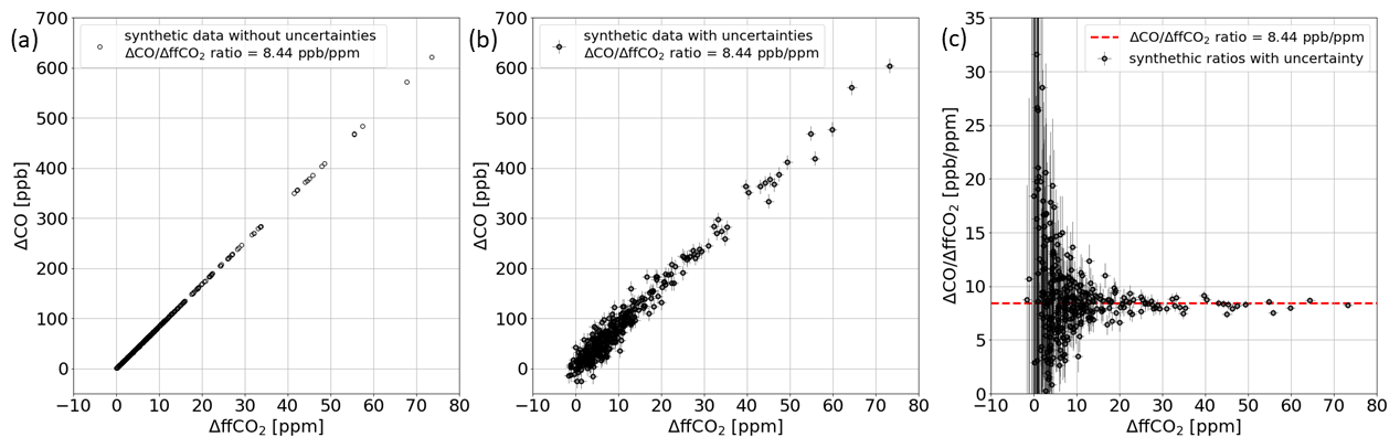
Figure A1 (a) Synthetic “true” ΔCO and ΔffCO₂ data with a constant ratio of 8.44 ppb ppm⁻¹. (b) Synthetic error-prone ΔCO and ΔffCO₂ data under the assumption of a constant ratio of 8.44 ppb ppm⁻¹. (c) Synthetic error-prone ΔCO $/$ ΔffCO₂ ratios.

For a comparison, we now can calculate the arithmetic mean, the error-weighted mean, and the median of the synthetic error-prone ratios as well as the slope of a weighted total least-squares regression line from Wurm (2022) using the synthetic error-prone ΔCO and ΔffCO₂ data. To get better statistics, we repeat this experiment 10 000 times. On average, we get the following results (average ± standard deviation over 10 000 repetitions):

• arithmetic mean of the ratios of 9.42 ± 77.84 ppb ppm⁻¹;

• error-weighted mean of the ratios of 8.24 ± 0.08 ppb ppm⁻¹;

• median of the ratios of 8.39 ± 0.11 ppb ppm⁻¹;

• slope of regression line of 8.44 ± 0.06 ppb ppm⁻¹.

This indicates that only the slope of a regression line, which considers the uncertainty of the ΔCO and ΔffCO₂ data yields the initial “true” constant ratio of 8.44 ppb ppm⁻¹. The arithmetic mean of the ratios shows the largest deviation from the “true” ratio, with a very large variability within the 10 000 repetitions. This can be explained by the wide scatter of the ratios during situations, with low ΔffCO₂ concentrations but huge relative ΔffCO₂ uncertainties. The respective error-weighted mean ratio and median ratio are 2.4 % and 0.6 % too low on average. This bias might be introduced by negative ratios, which are caused by very small synthetic “true” ΔCO or ΔffCO₂ data that became negative after adding the random uncertainty contribution. Therefore, we recommend using a weighted total least-squares algorithm to calculate the average < ΔCO $/$ ΔffCO₂ > ratio.

This synthetic-data experiment simulates the situation at an urban site like Heidelberg with a large range of ΔCO and ΔffCO₂ concentrations. In this case, we have a very good correlation between the ΔCO and ΔffCO₂ data. Indeed, the R² value from the applied regression is 0.968 ± 0.003 on average, while the uncertainty of the slope is 0.06 ppb ppm⁻¹ on average. However, what happens if we have a smaller range of ΔCO and ΔffCO₂ data, for example, at a remote site or during summer? To answer this, we perform the synthetic-data experiment again but only with synthetic “true” ΔffCO₂ concentrations that are smaller than 5 ppm. This increases the uncertainty of the slope to 0.55 ppb ppm⁻¹, which is almost a factor of 10 higher. Moreover, the R² value dramatically decreases to 0.08 ± 0.12. This shows the difficulty involved with calculating average ratios during summer or at very remote sites with low ΔffCO₂ signals (even in the absence of non-fossil CO sources).

In Sect. 3.1.2, we wanted to estimate the contribution of the observational uncertainties (i.e., the measurement and background representativeness uncertainty) to the RMSD between the ΔCO- and ¹⁴C-based ΔffCO₂ concentrations of the Heidelberg flasks. For this, we used the average flask < ΔCO $/$ ΔffCO₂ > ratio to calculate synthetic ΔCO-based ΔffCO₂ concentrations from the error-prone ΔCO data (see Fig. A1b). In Fig. 3b (red and orange dots for winter and summer flasks), we plot these synthetic ΔCO-based ΔffCO₂ data against the error-prone synthetic ΔffCO₂ concentrations.

A2 Summer versus winter ratios

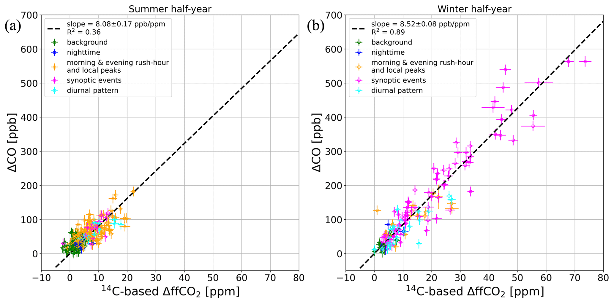
Figure A2 Scatterplot of the measured ΔCO and the ¹⁴C-based ΔffCO₂ concentrations of the hourly flasks collected at the Heidelberg observation site between 2019 and 2020 during (a) the summer half-year and (b) the winter half-year. The colors indicate the sampling situation of the flasks (see description in the caption of Fig. 2). The black dashed line shows a regression line performed with the weighted total least-squares algorithm from Wurm (2022).

A3 Simulated ΔCO and ΔffCO₂ contributions from the heating and traffic sectors

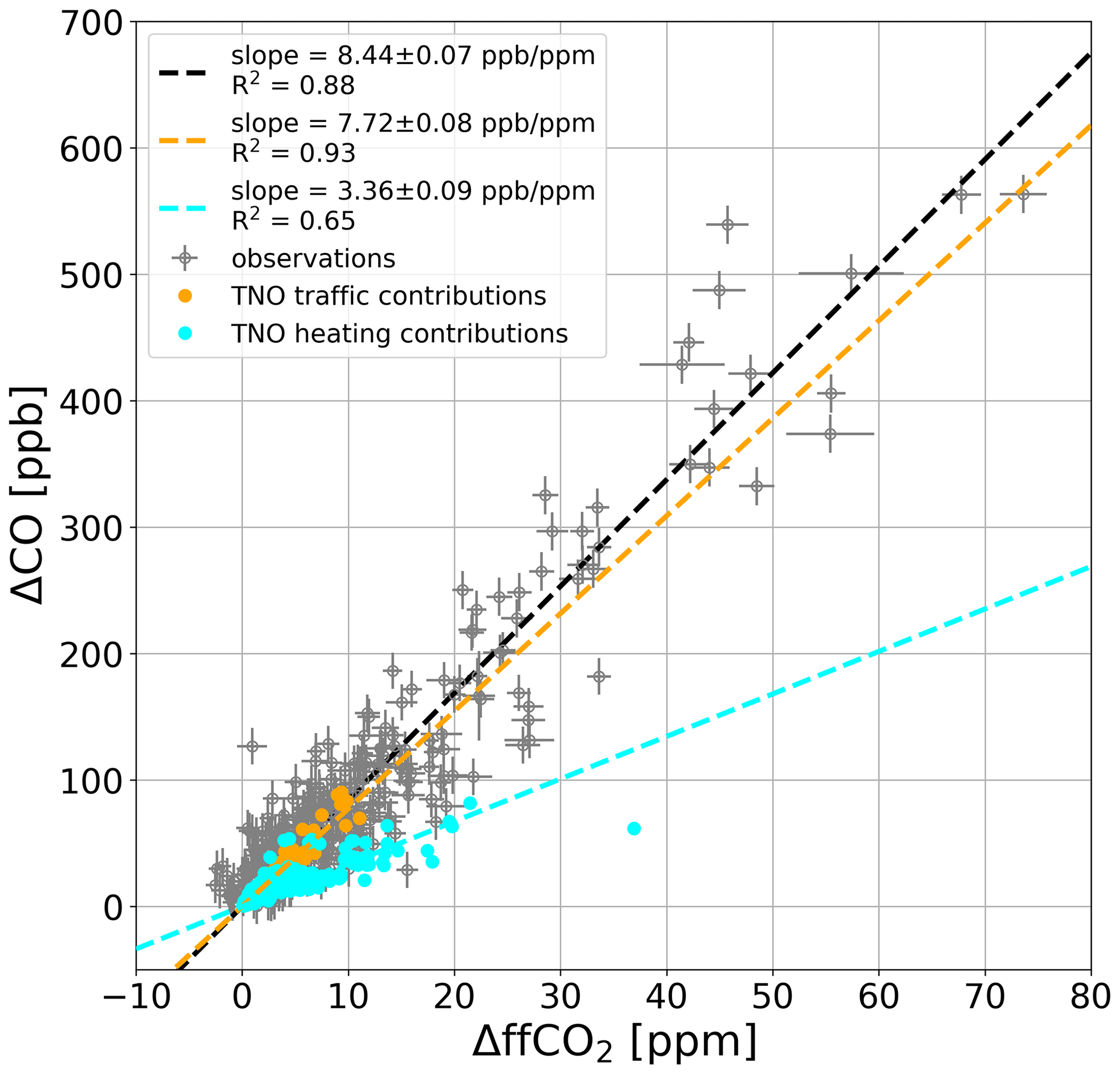
Figure A3 Simulated ΔCO and ΔffCO₂ contributions from the TNO traffic (orange) and heating (cyan) sectors for the Heidelberg flask events. The ΔCO and ΔffCO₂ concentrations of the Heidelberg flasks are shown in gray.