the Creative Commons Attribution 4.0 License.
the Creative Commons Attribution 4.0 License.
 | 12 Jul 2024
Vertical structure of a springtime smoky and humid troposphere over the southeast Atlantic from aircraft and reanalysis
Kristina Pistone
Eric M. Wilcox
Paquita Zuidema
Marco Giordano
James Podolske
Samuel E. LeBlanc
Meloë Kacenelenbogen
Steven G. Howell
Steffen Freitag
The springtime atmosphere over the southeast Atlantic Ocean (SEA) is subjected to a consistent layer of biomass burning (BB) smoke from widespread fires on the African continent. An elevated humidity signal is coincident with this layer, consistently proportional to the amount of smoke present. The combined humidity and BB aerosol has potentially significant radiative and dynamic impacts. Here, we use aircraft-based observations from the NASA ORACLES (ObseRvations of Aerosols above CLouds and their intEractionS) deployments in conjunction with reanalyses to characterize covariations in humidity and BB smoke across the SEA.
The observed plume–vapor relationship, and its agreement with the European Centre for Medium-Range Weather Forecasts (ECMWF) Reanalysis version 5 (ERA5) and Copernicus Atmosphere Monitoring Service (CAMS) reanalysis, persists across all observations, although the magnitude of the relationship varies as the season progresses. Water vapor is well represented by the reanalyses, while CAMS tends to underestimate carbon monoxide especially under high BB. While CAMS aerosol optical depth (AOD) is generally overestimated relative to ORACLES AOD, the observations show a consistent relationship between carbon monoxide (CO) and aerosol extinction, demonstrating the utility of the CO tracer to understanding vertical aerosol distribution.
We next use k-means clustering of the reanalyses to examine multi-year seasonal patterns and distributions. We identify canonical profile types of humidity and of CO, allowing us to characterize changes in vapor and BB atmospheric structures, and their impacts as they covary. While the humidity profiles show a range in both total water vapor concentration and in vertical structure, the CO profiles primarily vary in terms of maximum concentration, with similar vertical structures in each. The distribution of profile types varies spatiotemporally across the SEA region and through the season, ranging from largely one type in the northeast and southwest to more evenly distributed between multiple types where air masses meet in the middle of the SEA. These distributions follow patterns of transport from the humid, smoky source region (greatest influence in the northeast of the SEA) and the seasonal changes in both humidity and smoke (increasing and decreasing through the season, respectively). With this work, we establish a framework for a more complete analysis of the broader radiative and dynamical effects of humid aerosols over the SEA.
- Article
(8845 KB) - Full-text XML
-
Supplement
(1512 KB) - BibTeX
- EndNote


Aerosol effects on atmospheric radiative transfer and dynamics are complex and varied. Aerosols not only produce direct radiative heating or cooling, but may also alter the properties of nearby clouds by directly changing a cloud's reflectivity (albedo), thickness, or altitude; the total cloud amount; or the surrounding atmospheric dynamics. These effects are especially complex for absorbing aerosols such as biomass burning (BB) smoke. The combination of direct, indirect, and semidirect effects together may result in either an overall warming or a cooling effect (e.g., Koch and Del Genio, 2010) depending on the specific aerosol properties but also on the surrounding cloud, radiative, and meteorological context. A key consideration to understanding this aerosol–cloud–climate puzzle is the role of atmospheric water vapor, both in total amount and its location. Water vapor plays a significant role as a climate feedback parameter (e.g., Forster et al., 2021), has its own localized radiative heating effects, and is important to cloud formation and cloud lifetime in the present and future climate. Thus, it is important to consider how the local atmospheric properties may either affect or be affected by the combined presence of aerosols and water vapor. By characterizing these properties individually and together, we aim to understand the radiative and dynamic effects of humid and smoky air masses for a given region (here, the southeast Atlantic Ocean).
The atmosphere over the southeast Atlantic Ocean (SEA) is subjected to a consistent layer of biomass burning (BB) smoke from widespread fires on the African continent in the austral springtime (August through October). This smoke layer is initially lofted high in a continental mixed layer (∼ 5–6 km, ∼ 500–600 hPa) before being transported westward by the south African Easterly Jet (AEJ-S, ∼ 600–700 hPa) where it overlies and ultimately mixes into the stratocumulus-topped oceanic boundary layer. These conditions make the SEA an ideal location for studying the varied aerosol effects on climate. The NASA ORACLES (ObseRvations of Aerosols above CLouds and their intEractionS; Redemann et al., 2021) campaign was designed to study just that; in the present work, we use aircraft-based observations from the three ORACLES deployments, which (by design) spanned the spring BB season (September 2016, August 2017, and October 2018). Taken together, these data allow us to characterize the spatial and temporal variations in atmospheric chemistry, aerosol, and meteorological structure as the season progresses, specifically the covariations in humidity and aerosol. In a previous work (Pistone et al., 2021), we showed how observations from ORACLES-2016 exhibited a strong correlation between plume strength (i.e., carbon monoxide (CO) concentration and aerosol extinction) and water vapor specific humidity. This is consistent with previous work over the region; for example, Adebiyi et al. (2015) analyzed MODIS and radiosonde data (over St Helena, 15.9° S, 5.6° W) and found that increases in aerosol optical depth were associated with increases in mid-troposphere (700–500 hPa) moisture content, and the presence of humidity was noted even in southern African BB aerosol measurements in the Southern African Regional Science Initiative 2000 (SAFARI 2000) campaign (e.g., Haywood et al., 2003; Magi and Hobbs, 2003). More recently, Cochrane et al. (2022) used high-vertical-resolution aircraft data to quantify the aerosol and water vapor heating rates for specific case studies from ORACLES-2016 and ORACLES-2017. Both these recent studies concluded that there is significant shortwave water vapor heating coincident with the aerosol heating within the combined aerosol–humidity layer, despite longwave water vapor cooling.
The presence of humid smoke may have additional impacts on the lower atmosphere, including on the underlying stratocumulus clouds. Absorbing aerosols above the cloud layer have been found to suppress cloud-top turbulent fluxes, resulting in physically thicker clouds with a higher liquid water path (LWP) (e.g., Wilcox, 2010; Wilcox et al., 2016) and thus higher cloud albedo. In a modeling-based study, Ackerman et al. (2004) modeled the influence of above-cloud water vapor using several case studies informed by field measurements and concluded that the cloud liquid water path response to aerosol (i.e., increasing LWP due to precipitation suppression) had a much stronger response in the presence of overlying water vapor than under dry conditions due to changes in cloud-top entrainment. Deaconu et al. (2019) used satellites and reanalysis to conclude that absorbing aerosols in the SEA increased cloud optical thickness and liquid water path and lowered cloud-top altitudes. In a recent study using large eddy simulations, Baró Pérez et al. (2024) found that the moisture in the SEA BB affected the evolution of the underlying cloud field in addition to radiative effects of the humid BB plume.
Pistone et al. (2021) also presented evidence that the smoke–humidity relationship is present at the air mass origin over the African continent, thus indicating that these air masses are likely subjected to the combined effects of humidity and BB aerosols for an extended time. In other words, the humid atmosphere observed over the SEA is subjected to not just instantaneous but cumulative direct and semi-direct effects of the layer of BB aerosol, from the time it took a given air mass to leave the continent to when it was measured by the ORACLES flights (on the order of a few days to weeks from origin to observation), above and into the cloud layer. Within our current context, it is important to recognize that the humidity of the above-cloud air will influence the magnitude of aerosol-forced dynamical effects on clouds. From a practical measurement standpoint, humid aerosols also undergo swelling which affects their remote sensing retrievals and comparisons with modeled results (e.g., Shinozuka et al., 2020; Doherty et al., 2022). By combining aircraft data with large-scale reanalyses, we aim to characterize the variations in water vapor in conjunction with BB aerosol over the springtime southeast Atlantic region, which allows us to assess the realism of the reanalysis datasets commonly used to initialize and constrain model simulations and to conduct broader studies of the region as a whole.
There are three major goals of this paper. First, to expand the results of Pistone et al. (2021) in order to discuss how the observed patterns in water vapor and CO vary across the three ORACLES observation periods, which by design sampled different times during the BB season. Second, to assess how well selected reanalysis products capture the results in the observations. Third, to describe a new method for using climatological data to more completely characterize the atmospheric structure over this region and its radiative impacts.
Section 2 describes the observations and reanalyses used in this work. In Sect. 3 we extend the findings of Pistone et al. (2021) to describe the observations from the three deployment years, including a new discussion of the Copernicus Atmosphere Monitoring Service (CAMS) reanalysis and the climatological representativity of its BB tracers, specific humidity, and aerosol parameters. In Sect. 4, we describe our use of a k-means clustering of the European Centre for Medium-Range Weather Forecasts (ECMWF) Reanalysis version 5 (ERA5) and CAMS reanalysis to identify canonical atmospheric profile types of varying atmospheric specific humidity (q), carbon monoxide (CO), and vertical structure and then describe their changing (co)incidence spatially and throughout the season. Section 5 discusses the broader significance of this analysis within the context of previous works on this topic. With this work, we describe more completely the atmospheric structure of smoke and humidity over the SEA and lay out a framework for further analysis of the radiative and dynamical impacts of this humid plume over time and space, including its effects on clouds and climate.
In the present work, we use aircraft observations from ORACLES in conjunction with data from the ERA5, CAMS, and MERRA-2 (Modern-Era Retrospective Analysis for Research and Applications, version 2) reanalyses.
2.1 Aircraft instrumentation
The ORACLES field mission consisted of three deployments: September 2016 out of Walvis Bay, Namibia; August 2017 out of São Tomé, São Tomé and Príncipe; and October 2018 also out of São Tomé. All instruments used here were deployed on the NASA P-3 aircraft during all three ORACLES deployments. The archived 1 Hz measurements are used unless otherwise indicated. A detailed description of the ORACLES experimental construction and instrumentation used here may be found in Redemann et al. (2021) or in the archived instrument dataset metadata (see “Code and data availability”).
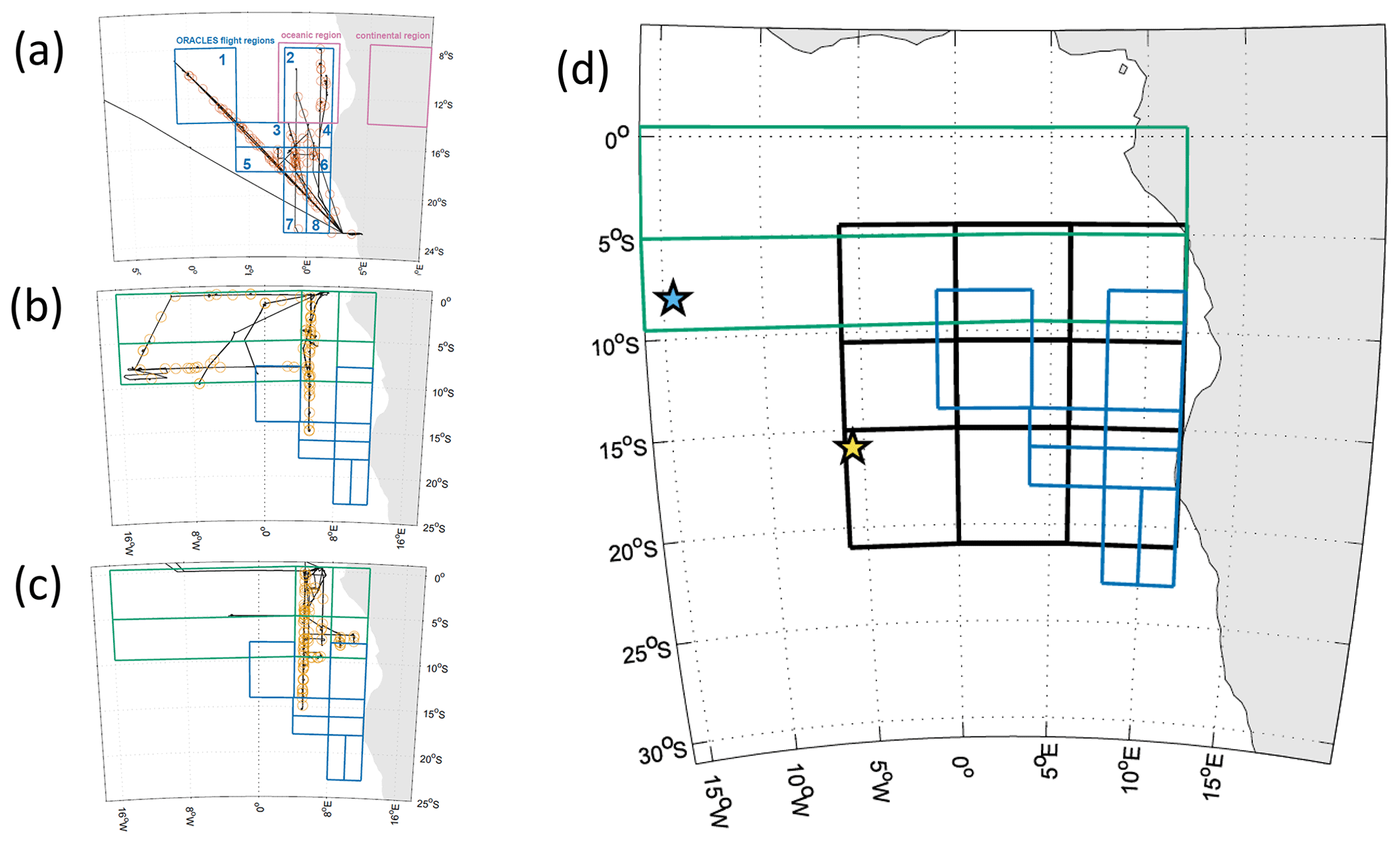
Figure 1Regional distributions of observations and the spatial subdivisions used. (a) From Pistone et al. (2021): the locations of ORACLES-2016 aircraft profiles (orange circles), the regions used for the aircraft-based analysis (blue), and the reanalysis study (lavender). More northern profiles were sampled in (b) ORACLES-2017 and (c) ORACLES-2018. For ease of comparison, these data (green grid) are divided at 5° S to aid comparison with 2016 (blue grid). Note also the larger westward range of observations in 2017. (d) Summary of the different subdivided regions considered in this and other works. The stars show the sites of previous island-based observations at St Helena (yellow star) and Ascension Island (blue star). The thicker black lines are the SEA divisions discussed in Sect. 4, on a nominally 6° × 6° grid which is slightly uneven north-to-south to align with the CAMS spatial resolution and to isolate the AEJ-S latitudes.
Unless otherwise noted, the present analysis focuses on aircraft profile data during each ORACLES deployment, with the 1 Hz aircraft data averaged within 100 m (±50 m) of the reanalysis pressure levels. The locations of these profile data are presented in Fig. 1a–c, showing the locations of 105, 70, and 80 full or partial profiles (ramps or square spirals) sampled during the 2016, 2017, and 2018 campaigns, respectively. Spatial subdivisions used in previous works, as well as the framework for the present analysis, are illustrated in Fig. 1d. Due to the more northern deployment of ORACLES-2017 and -2018, the data shown in Sect. 3 are subselected to observations south of 5° S, in order to isolate air masses influenced by the AEJ-S (Pistone et al., 2021).
2.1.1 Inlet-based carbon monoxide and water vapor
In all ORACLES deployments, volume mixing ratios of carbon monoxide (CO), carbon dioxide (CO2), and water vapor (q) were measured by a Los Gatos Research CO/CO2/H2O Analyzer (COMA) modified for flight operations. It uses off-axis integrated cavity output spectroscopy (ICOS) technology to make stable cavity-enhanced absorption measurements of CO, CO2, and H2O in the infrared spectral region – technology that previously flew on other airborne research platforms with a precision of 0.5 ppbv over 10 s (Liu et al., 2017; Provencal et al., 2005). Water vapor measurements of less than 50 ppmv (∼ 0.03 g kg−1) were removed due to instrument signal limitations, but this has minimal effect on the data considered here.
In Pistone et al. (2021), we discussed the validation of COMA measurements against two other onboard water vapor and inlet-based gas/aerosol instruments on the payload; following the good agreement shown in that work, the specific humidity measurements presented here are from COMA. We focus on carbon monoxide as a BB tracer because it is a more straightforward parameter to accurately model and, as will be shown, agrees well with observed aerosol extinction across the three deployments.
2.1.2 Aerosol optical depth
The Spectrometer for Sky-Scanning Sun-Tracking Atmospheric Research (4STAR; Dunagan et al., 2013) is an airborne hyperspectral (350–1700 nm) sun photometer which measures direct-beam solar irradiance (sun-tracking mode) for retrieval of column aerosol optical depth (AOD; e.g., Shinozuka et al., 2013) and column trace gases (e.g., Segal-Rosenheimer et al., 2014) above the aircraft level. This work presents the column AOD (LeBlanc et al., 2020); we note that Pistone et al. (2021) also utilized 4STAR column water vapor (CWV) measurements in a similar analysis of the aerosol–water vapor coincidence. Measurement uncertainty in AOD is around 1 % (0.01 at 500 nm at solar noon), increasing in some cases to 0.03–0.04 due to aerosol deposition on the instrument's viewing window. An account of 4STAR measurement uncertainties is described in more detail in LeBlanc et al. (2020) and is provided in the data archive for the 1 Hz data.
2.1.3 Aerosol extinction
The Hawaii Group for Environmental Aerosol Research (HiGEAR) operated several in situ aerosol instruments on the P-3. Total and submicrometer aerosol light scattering coefficients (σscat) were measured on board the aircraft using two TSI model 3563 3-wavelength nephelometers (at 450, 550, and 700 nm) corrected according to Anderson and Ogren (1998). The scattering used here is from TSI Nephelometer #1 (as identified in the ORACLES dataset) measuring total aerosol scattering and interpolated to the PSAP absorption wavelengths (below). Aerosol extinction is the sum of PSAP absorption plus nephelometer scattering.
Light absorption coefficients (σabs) at 470, 530, and 660 nm were measured using two Radiance Research particle soot absorption photometers (PSAPs). We use absorption from the “Front” PSAP. The humidity within the PSAP was not explicitly controlled, but the PSAP optical block was heated to approximately 50 °C to reduce artifacts which would result from a changing RH; this had the effect of reducing relative humidity in this instrument to much lower than the 40 % within the nephelometers. The PSAP absorption was corrected using the wavelength-averaged correction algorithm (Virkkula, 2010) following the conclusions of Pistone et al. (2019). Instrument noise levels are 0.5 Mm−1 for a 240–300 s sample average, comparable to values reported previously (Anderson et al., 2003; McNaughton et al., 2011).
2.2 Large-scale reanalyses
In considering the reanalyses, we use specific humidity (q), carbon monoxide (CO), and aerosol optical depth (AOD) fields for the following subsets and resolutions.
The European Centre for Medium-Range Weather Forecasts (ECMWF) has developed global atmospheric reanalysis products for several decades, with ERA5 (ECMWF Reanalysis version 5) being the current product (Hersbach et al., 2020). In the comparison with ORACLES flights, we consider ERA5 at 0.25°, hourly resolution, at pressure levels of 50 hPa intervals between 400 and 750 hPa and 25 hPa intervals from 750 to 1000 hPa, and we use 0.25°, 3-hourly resolution in the k-means analysis. ERA5 does not report atmospheric chemistry or aerosols nor does it assimilate observed aerosol datasets, although satellite measurements of (aerosol-influenced) radiances are assimilated into the reanalysis (Hersbach et al., 2020). In a slight difference from Pistone et al. (2021), here we add the 400 hPa level (approx 7.6 km) to our analysis to better align with the CAMS reanalysis (below) which reports at 400 hPa rather than 450 hPa; our previous work only extended to 450 hPa (roughly 6.7 km), which was chosen to capture the full BB plume height and ORACLES P-3 aircraft operating altitudes, but the impacts on the statistical results are seen to be minimal.
For analysis of aerosol/chemistry parameters, we consider the Copernicus Atmosphere Monitoring Service (CAMS) reanalysis. CAMS includes chemistry but is coarser than ERA5 both spatially and temporally, namely, 3-hourly versus hourly, 0.75° versus 0.25°, and 10 pressure levels from the surface to 400 hPa rather than 18 levels (100 hPa intervals in the plume level). CAMS uses the same meteorological inputs as does ERA5, assimilates MOPITT (on NASA's Terra satellite) CO retrievals (among other chemistry), and includes radiatively active aerosol fields (Inness et al., 2019). While total AOD (from MODIS on both NASA's Terra and Aqua satellites, for our study period) is assimilated into CAMS from satellite observations, the model aerosol scheme uses 12 speciated aerosol tracers (in specific prescribed size bins, hydrophobic/hydrophilicity state, and treated as externally mixed), which likely leads to less-constrained aerosol results compared with those for trace gases (Inness et al., 2019).
The Modern-Era Retrospective Analysis for Research and Applications, version 2 (MERRA-2) is an atmospheric reanalysis produced by NASA's Global Modeling and Assimilation Office (GMAO) (Gelaro et al., 2017; Randles et al., 2017; Buchard et al., 2017). MERRA-2 assimilates observations of meteorological parameters from multiple satellite platforms, as well as aerosol optical depth from satellites (MODIS, AVHRR) and ground-based (AERONET) measurements, into a comprehensive atmospheric model, with explicit accounting of aerosol radiative effects. MERRA-2 datasets are given on a nominal 50 km horizontal resolution (0.5° × 0.5°) with 72 vertical layers from the surface to 0.01 hPa, and the complete set of MERRA-2 files have additionally been sampled up to 1 s resolution along every ORACLES flight (Collow et al., 2020). Our analysis here subsets this product to the same ERA5 pressure levels for ease of interpretation. While the focus of later sections is on CAMS and ERA5, MERRA-2 results from 2016 were discussed in Pistone et al. (2021); for completeness, in Sect. 3 we thus also discuss this product over all ORACLES deployments.
For sections where the observations are compared with reanalyses, the 1 Hz aircraft observations are averaged within 100 m (±50 m) of the reanalysis pressure levels. The comparisons with the ECMWF reanalyses are first paired to the closest reanalysis time step to the profile mean time and then the nearest-neighbor latitude and longitude to the mean profile locations so as to maintain consistency with the later sections focused solely on reanalysis fields. We note that the results presented here are consistent for subsets of the data considering either solely square spiral profiles (i.e., the more spatially localized profiles) or profiles with the greatest temporal collocation (< 1 h).
In assessing the representativeness of the reanalyses and their agreement with the ORACLES observations, we focus on the parameters of specific humidity, the biomass burning tracer CO, and both column and inlet-based aerosol extinction.
3.1 Water vapor and BB tracer (CO)
We begin our analysis with specific humidity q, a meteorological field, and CO, a biomass burning tracer. We choose CO as our BB tracer because the modeling of chemical species is subjected to fewer uncertainties than is aerosol modeling. Aerosol as modeled in the CAMS reanalysis considers aerosol speciation, processing, lifetime, and removal for 12 separate aerosol components, while the assimilated observation is column total AOD from satellites (Inness et al., 2019). Because of this, we expect CO to have a more straightforward and accurate representation than the fields of aerosols themselves for our purposes of assessing and characterizing atmospheric distributions over time. We note that the lifetime of CO in the atmosphere is 1–4 months (Szopa et al., 2021) and thus may result in accumulation to a higher background value over the span of a given biomass burning season (3 months); but as we show in Sect. 3.2, the observed aerosol–CO relationship does not vary across the three airborne campaigns.

Figure 2Scatterplots of water vapor and CO for September 2016 and by altitude, showing data collected during P-3 aircraft vertical profiles (circles in Fig. 1a). Comparisons are shown for the (a, f) ERA5, (b, d, g) CAMS, and (c, e, h) MERRA-2 reanalyses. (a–c) Observed water vapor (averaged over a 100 m layer) compared with coincident reanalysis values. (d–e) Observed CO compared with the same for CAMS (d) and MERRA-2 (e). (f–h) Collocated CO versus water vapor for each product (aircraft observations, CAMS, and MERRA-2). Blue squares = 1000–875 hPa (surface to ∼ 1.3 km; boundary layer); yellow triangles = 850–750 hPa (∼ 1.5–2.6 km; BL top/transition); orange circles = 700–400 hPa (∼ 3.2–7.6 km; BB plume). The 1 : 1 line is shown as a dashed black line. The total least-squares fits for data > 2 km are shown as a dashed gray line and the corresponding values of fits and correlations are given in Table 1.
Previous work by Pistone et al. (2021) showed that the ERA5 reanalysis captured the vertical structure and location of the humid plume remarkably well in September 2016 (there reported as an observed–ERA5 correlation of R2=0.79 for observations above 2 km over all flights). ERA5 performed better than MERRA-2 in terms of this direct comparison (observed–MERRA-2: R2=0.40) due to a known vertical velocity (excessive subsidence) issue in the latter (e.g., Das et al., 2017). Figure 2 shows comparisons between (left, middle, right) ERA5, CAMS, and MERRA-2 versus the observed values from the 2016 ORACLES deployment for (top, middle, bottom) specific humidity, CO, and the relationship between the two. The CAMS reanalysis shows a similar pattern in specific humidity and agreement with the observations (R2=0.84 for z≥2 km) despite its lower resolution (Sect. 2) giving roughly half as many matches compared with ERA5. In all the reanalyses considered, the largest reanalysis–observation discrepancies occur near the top of the boundary layer (∼ 1–2 km).

Figure 3As in Fig. 2, but for August 2017. Data shown here are from profiles south of 5° S (Fig. 1b) to isolate the air masses influenced by the AEJ-S, although the results are consistent for the larger dataset. The bottom left (observed CO versus water vapor) illustrates the greater range in CO values as compared with 2016.

Figure 4As in Fig. 2, but for October 2018. Data shown here are from profiles south of 5° S (Fig. 1c), although the results are consistent for the larger dataset. Here, the most striking feature is the lower-CO and higher-q conditions (i.e., steeper slope in the bottom row) as compared with observations from earlier in the BB season.
For the CO comparisons (Fig. 2, middle row), there is similar good agreement overall between CAMS and observations (R2=0.75 for z≥2 km) although the reanalysis tends to underestimate these values for higher observed CO (≳ 300 ppb; this is also seen in individual profiles, as shown in Fig. S1 in the Supplement). The overall slope between the CAMS and observed CO is 0.79 (i.e., showing underestimation) compared with 0.98 for the CAMS q versus observed q. Still more variability is seen in the direct comparison with MERRA-2 (CO observed–MERRA-2 correlation: R2=0.21). This general pattern is consistent over all three ORACLES deployments (Figs. 2, 3, and 4) and is also consistent with Pistone et al. (2021), most likely due to the aforementioned issue with vertical plume displacement. In other words, MERRA-2 tends to underestimate the higher-altitude points while sometimes overestimating lower-altitude points for both CO and q relative to aircraft observations, but it preserves the relationship between CO and q for MERRA-2 overall (e.g., Fig. 2, bottom right).
Table 1R2 values, total number of matched observations, and total least-squares linear fits for aircraft and reanalysis data. Data are shown for the subset matching the profiles in Fig. 1 and are for altitudes of 2 km and above (i.e., 800–400 hPa levels) and south of 5° S for 2017 and 2018 (i.e., AEJ-S-influenced latitudes). The left columns show correlations between specific humidities, while the right side shows the correlations for CO. All R values are statistically significant at p<0.0001.
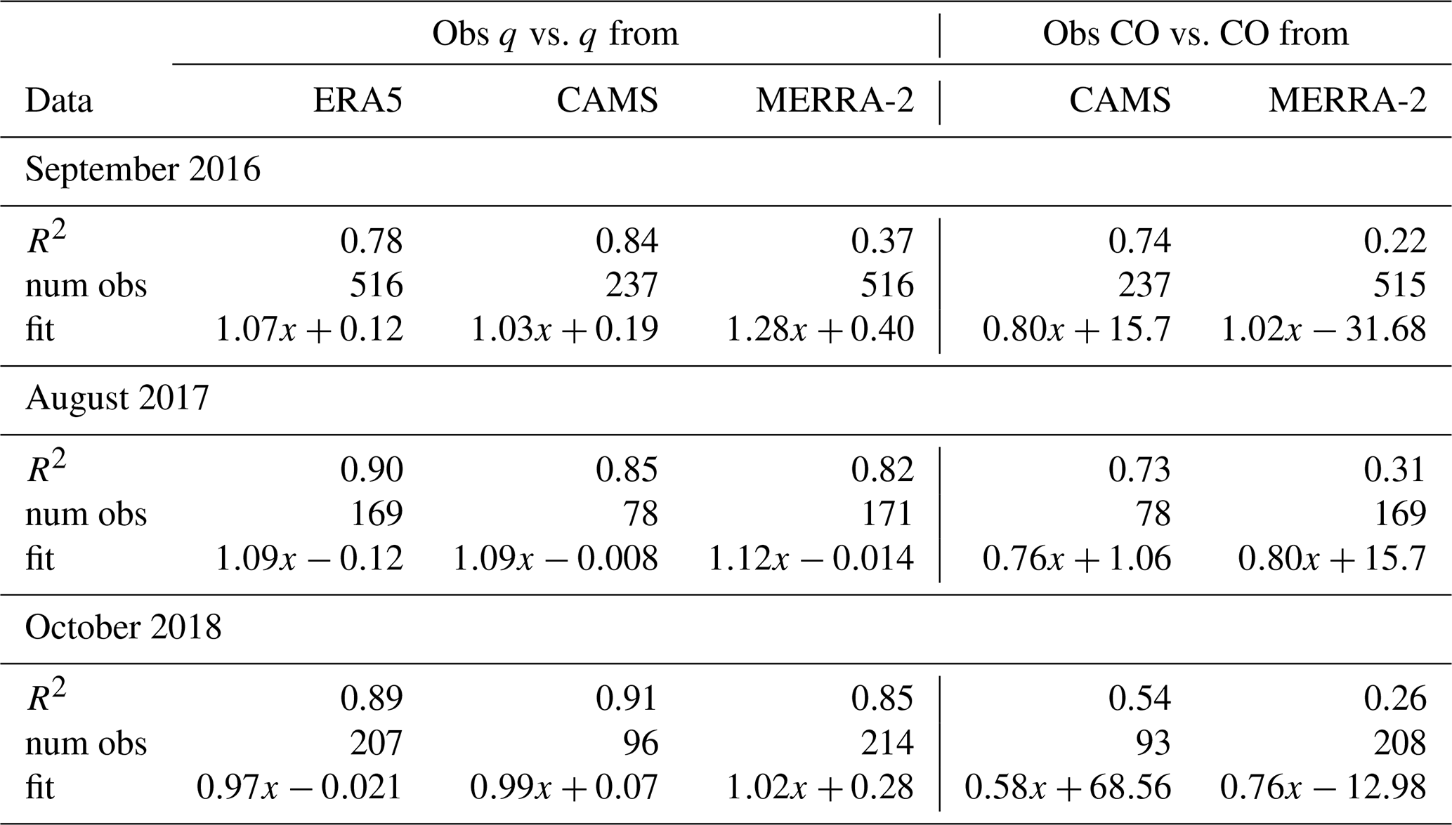
The data from August 2017 (Fig. 3) and October 2018 (Fig. 4) are largely consistent with those from September 2016, with a few notable differences. First, the correlations of observed versus CAMS or ERA5 water vapor are slightly better than in 2016 and substantially better for MERRA-2 (Table 1; with the caveat that there are fewer profile matches for these years). However, the observed versus CAMS CO is a somewhat poorer match both in terms of the R2 values and the slope for the latter deployments. (All correlation coefficients are statistically significant at the p<0.0001 level.) This difference in correlations between the three deployments may be partly explained by the seasonal evolution of the smoke plume; specifically, higher CO observed in August 2017 results in a slope which is skewed low due to the CAMS high CO underestimation, and the lower CO observed in October 2018 results in a less robust (i.e., lower) R2 value due to a smaller dynamic range in CO values. It is also possible that there are differences in the emissions inventory assimilated into CAMS for each month of the BB season, although such diagnostics would be beyond the scope of this paper.
In addition to the direct comparisons between observations and reanalyses, Figs. 2–4 also show how the correlation between CO and q is represented by each entity (bottom row). The differences between plume level (orange circles) values versus PBL observations (blue squares) are evident (i.e., humid but low-CO air masses are found only in the oceanic PBL), but overall these relationships continue to be well represented, despite the mismatch in location for some reanalyses versus observations (e.g., the displacement in MERRA-2). As was discussed briefly in Pistone et al. (2021), the magnitude of the observed CO–q relationship varies across different deployments/months (from observations, slopes were 0.020, 0.023, and 0.05 (g kg−1) ppb−1 for August, September, and October, respectively), due in large part to the changing meteorological and BB conditions, namely, the increase in humidity and decrease in BB loading as the season progresses (Adebiyi et al., 2015; Ryoo et al., 2022).
In light of the better CAMS and ERA5 agreement with observations compared with MERRA-2, in the subsequent sections we focus our analysis on the ECMWF reanalyses (higher-resolution ERA5 for water vapor, and CAMS for chemistry).
3.2 Aerosol loading and aerosol optical depth
Ultimately, our interest in characterizing the atmospheric structure in this region stems from a desire to understand and quantify the aerosol radiative and dynamic effects of the BB plume. We have focused on a BB tracer field from the reanalyses (i.e., CO) because, due to the complexities in atmospheric aerosol processing in the real world and in models, CO is a simpler parameter to model accurately compared with speciated aerosol. Of course, this exercise will be only tangential to the radiative question if the CO tracer does not correspond to aerosol loading in the real world. To explore whether this is the case, Fig. 5 shows the aircraft-observed CO versus extinction (nephelometer scattering plus PSAP absorption; Sect. 2.1.3) subset to the same profiles as Figs. 2–4. There are a few outlier points in 2016 (during this deployment, the nephelometer had an issue with dead air when entering or exiting the plume altitudes), but overall the correlations are strong (R2>0.9 for 2017 and 2018 and R2=0.83 for 2016). Importantly, the slopes themselves are consistent year to year (dashed lines; total least-squares fit slopes of 1.20–1.28 over the 3 months) suggesting the CO–aerosol extinction relationship does not exhibit a significant seasonal dependence, at least for these dried, inlet-based measurements.
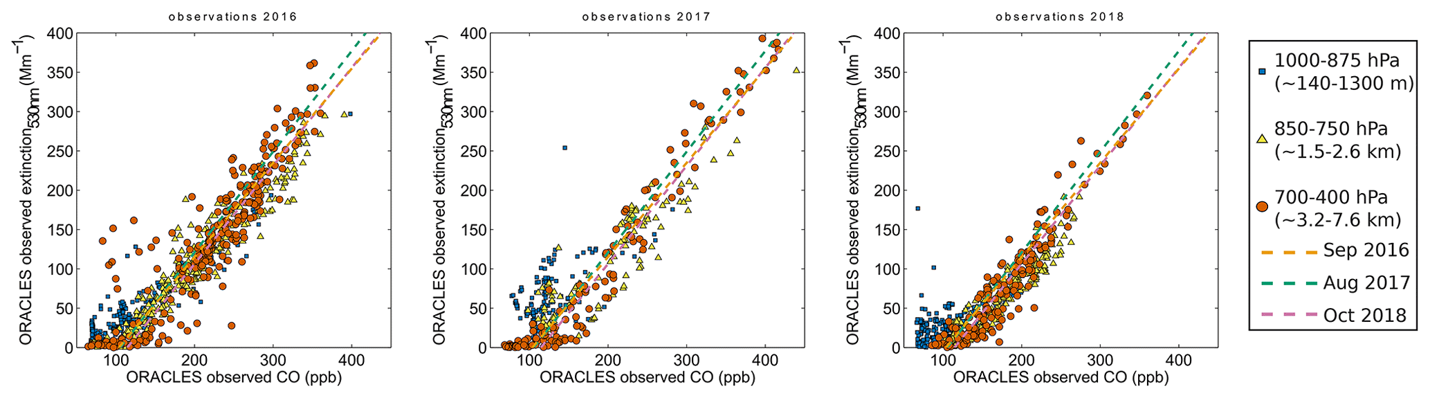
Figure 5Inlet-based observed CO and aerosol extinction (in situ scattering plus absorption) for ORACLES deployment for the same profiles shown in Figs. 2–4. The R2 correlations are > 0.9 for plume level (> 700 hPa) for 2017 and 2018 and R2=0.83 for 2016. The lower 2016 correlation was due to issues with dead air in the nephelometer which produced artifacts while profiling during that deployment. Lines show the total least-squares fit to all data above 3 km for each year, and the relationship is consistent throughout the season (slopes of 1.20–1.28) despite variability in loading.
Figure 6 shows comparisons between 4STAR-measured AODs and CAMS AOD (both at 550 nm) for the same profile locations. Note that we show both reported “total” CAMS AOD as well as the sum of the CAMS-reported organics and BC components of AOD to isolate the BB plume signal from potential other sources such as sea salt. Sea salt in particular is likely to be excluded from much of the ORACLES AOD measurements, which only include above-aircraft column AOD due to 4STAR viewing geometry.

Figure 64STAR to CAMS for 2016 (a, b), 2017 (c, d), and 2018 (e, f) deployments at the location of aircraft profiles (Fig. 1) for total (a, c, e) and BB-only (b, d, f) CAMS AODs. Colors indicate the altitude of the aircraft measurement (i.e., the lowest value in the given aircraft profile); the observed AOD is for the column above this altitude compared with the full-column values reported by CAMS. Dashed lines show the 1 : 1 line.
Figure 6 shows the variation in correlations and spreads for the different deployments. Contrasting the years, we see a poorer correlation and greater spread in CAMS-4STAR differences in September 2016 compared with later years (direct differences and their distributions are shown in Figs. S2 and S3). Table 2 summarizes the correlations, slopes, and agreement between the observations and the CAMS BB AOD. All years share some features: for all years, using only BB aerosol types in CAMS brings the average more in line with the observations compared with “total” AOD, but this offset is reasonably consistent across all data. Also, in all years, particularly for higher loading conditions, CAMS tends to overestimate AOD relative to 4STAR, a curious feature since, as shown previously, CAMS tends to underestimate CO concentration particularly for higher loadings (Figs. 2–4). As noted in Sect. 2.2, the assimilated satellite-observed aerosol is total-column AOD, whereas CAMS aerosol is partitioned into a speciated model, with aerosol and chemistry largely independent of one another (Inness et al., 2019), and then summed to column AOD. Because of this and previous results showing that total AOD from MODIS in this region is greater than that observed from aircraft due to the difficulties in retrieving above-cloud aerosol (LeBlanc et al., 2020), it is not surprising that CAMS overestimates AOD relative to the aircraft observations, as the CAMS AOD is a less constrained parameter than CO.
Table 2Agreement between CAMS AOD (organic and BC) and 4STAR ACAOD for the profiles shown in Fig. 1 from each ORACLES deployment. All correlation coefficients are significant at p<0.0001.
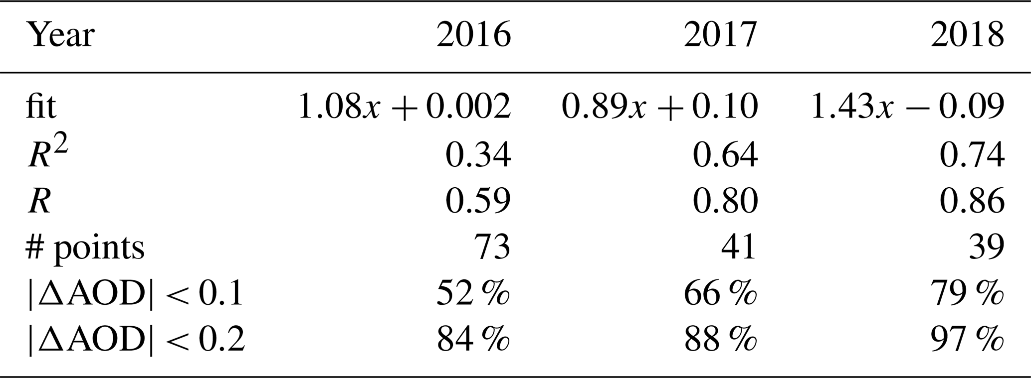
Regardless, the majority of the available comparisons agree within AOD ± 0.2 of one another (Table 2; Figs. S2, S3), despite the tendency of CAMS to overestimate AOD relative to 4STAR in all years, even when only BB AOD is considered. We note that Cochrane et al. (2022) found that the aerosol heating rate increased by ∼ 0.5 K d−1 per 0.1 increase in AOD, suggesting that it is worth further characterizing the nature and impacts of a disagreement of this magnitude. Potential sources of uncertainty from the 4STAR measurements include only partial columns due to aircraft altitude; indeed, it is particularly evident in the 2016 and 2017 panels of Fig. 6 that the higher altitudes (yellow points, i.e., a smaller fraction of a “full column”) tend to show the largest negative deviations compared with CAMS, possibly due to 4STAR missing below-aircraft AOD contributions. Differences in spatial sampling may also contribute to the year-to-year differences.
In terms of column aerosol measurements, Pistone et al. (2019) demonstrated that 4STAR AODs, while generally consistent with other measurements of optical depth, tended to be slightly larger than co-located values by other measurement methods (there, integrated column extinction from inlet-based instruments and remotely sensed measurements from downward-looking sensors), most likely due to the differences in viewing geometry. Chang et al. (2021) showed good agreement both between the 4STAR AOD and HSRL-2 AOD products, and between 4STAR and several satellite-derived (MODIS and SEVIRI) ACAOD products, for conditions of close temporal collocations. Under more relaxed temporal agreement constraints, when compared with the two different MODIS ACAOD algorithms, 4STAR tended to report slightly lower ACAOD than one and slightly higher than the other. The authors concluded that these results suggested aerosol loading conditions over the SEA can vary substantially within a 3 h period, which may also help to explain the poorer agreement of the 3-hourly CAMS reanalysis relative to the hourly ERA5 results for q, although the AOD results in Fig. 6 are not altered by excluding profiles with the greatest temporal mismatch between reanalysis and flights.
Interestingly, when we consider CAMS column CO versus column BB (organics plus BC) AOD, the relationship does vary with season (example shown in Fig. S4). For each of the deployments in the years 2016–2018, the October data show a steeper slope (i.e., more AOD per unit CO) than do the earlier months, similar to the pattern shown in Fig. 2 versus Fig. 4. This is not inconsistent with Fig. 6, considering the contributions of the boundary layer to modeled column values, and this could potentially also be affected by aerosol hygroscopicity, which is included in the CAMS aerosol scheme (Inness et al., 2019; Morcrette et al., 2009) and which would likely be more prominent in the more humid October months. We note that Shinozuka et al. (2020) concluded that 90 % of free tropospheric ORACLES-2016 measurements were not significantly affected by hygroscopic swelling (f(RH)<1.2) although hygroscopicity effects were more pronounced in PBL measurements (f(RH)>2.2 for half the valid inlet-based measurements). Hygroscopic swelling would not be a factor in the inlet-based aircraft measurements (Fig. 5) which were dried to RH < 40 %. Overall, these considerations complicate studies using modeled or observed aerosol extinction, which explains our approach of using a CO tracer, while also emphasizing the importance of field measurements in the region.
Despite the considerations discussed above, our analysis shows a general good agreement between the ORACLES aircraft data and the ERA5 and CAMS reanalyses from all three deployments. These products are thus useful to the end goal of a more complete characterization of the atmospheric structure of the region as a whole. We approach this section with the goal of being able to characterize the frequency of profiles over the SEA region as a whole and climatologically during the BB season, beyond solely during flight periods and locations.
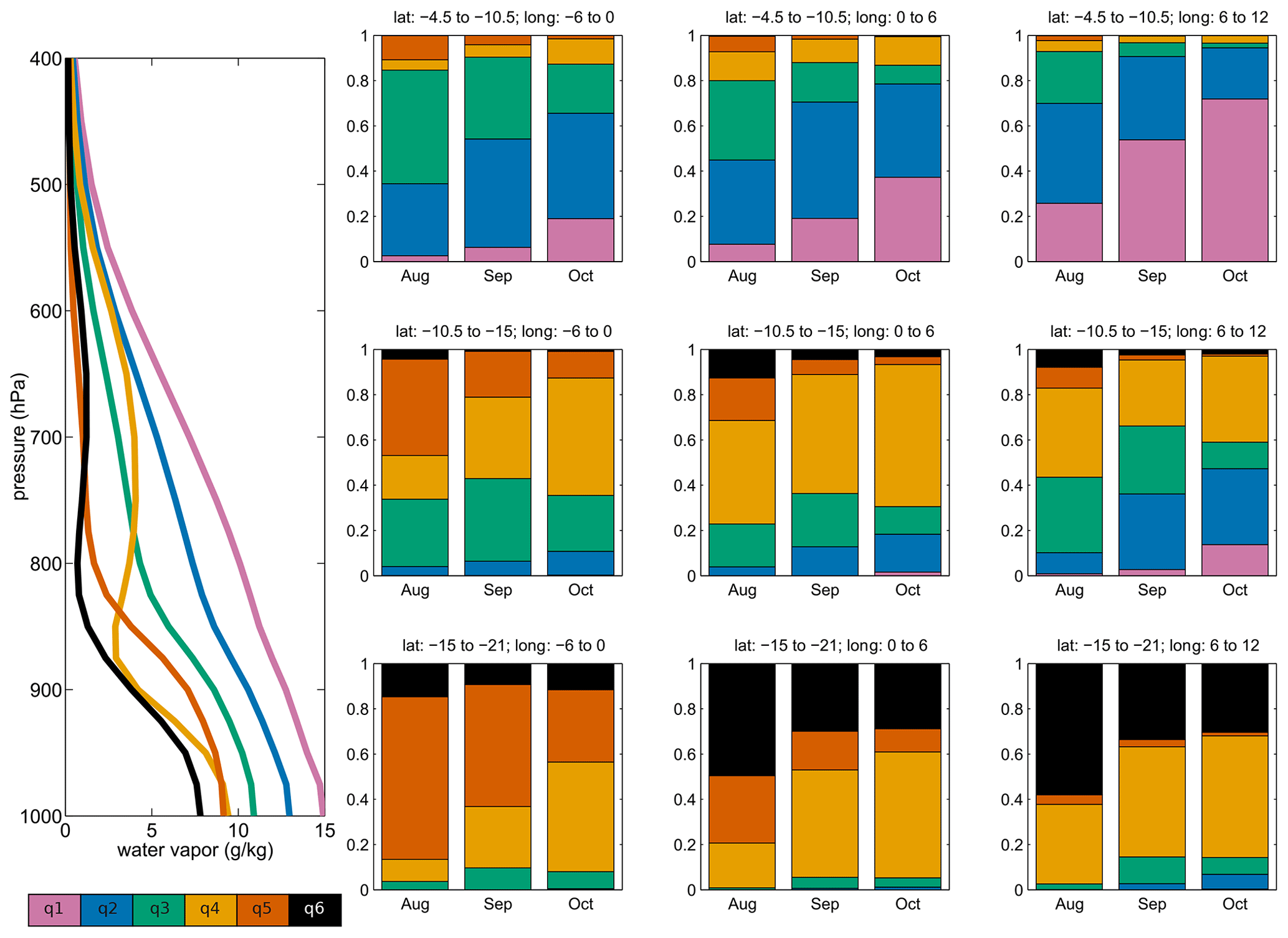
Figure 7The six k-means profile types determined from ERA5 reanalysis water vapor (left). Fractional incidence of k-means water vapor classifications, by month, for ERA5 August–October 2014–2020 (right). The grid corresponds to the black outlines in Fig. 1d. Note that the top and middle rows correspond to the AEJ-S latitudes (5–15° S), with the top row is slightly extended to align with the CAMS 0.75° resolution used in Fig. 8.

Figure 8The six k-means profile types determined from CAMS reanalysis CO (left). Fractional incidence of k-means CO classifications, by month, for CAMS 2014–2020 for the regions shown in Fig. 1d (black grid).
To accomplish this, we performed a k-means cluster analysis, similar to the methods used by Schelbergen et al. (2020), on the full reanalysis subset of 3-hourly August, September, and October data from 2014 through 2020, from the Equator to 30° S and 15° W to 12.5° E (i.e., close to the coast without including land). We use vertical pressure levels between 1000 to 400 hPa, giving 18 levels of q from ERA5 and 10 levels of CO from CAMS. First we perform a principal component analysis separately for q and CO by decomposing the full set of all profiles for each variable into two principal components describing the variability of the profiles. The ranges of values classed into each profile cluster are shown in Fig. S5 and the principal components are shown in Figs. S6 and S7. Then the distribution of ERA5 profiles in the phase space of the two principal components is passed to a k-means clustering algorithm to arrive at a set of canonical profiles for each variable. For each variable, six clusters (shown in Figs. 7 and 8) were determined from the two principal components, whose variability corresponded to (1) total concentration (i.e., profile q1 vs. q2 vs. q3) and (2) the ratio of upper-level (∼ 600–700 hPa) to lower-level (∼ 900 hPa) values (i.e., q1 vs. q4 vs. q6; distributions varying across each of the two principal components for q and CO are shown in Figs. S8–S11). The profile labeling corresponds roughly to the column concentration, i.e., q1 is the most humid and q6 is the driest; C1 has the highest CO concentrations and C6 has the lowest. We chose a six-cluster configuration because with this number we were able to adequately capture the variability of conditions (described below) while limiting the number of defined profiles for ease of interpretation. ERA5 outputs subsampled to the CAMS spatial resolution produce similar results, and the k-means cluster method produces similar results (i.e., the same general types and range of profile types) for slight differences in the spatial domain of the data used in the analysis and for the number of clusters chosen. A silhouette analysis of various configurations between three and nine clusters suggests the addition of more clusters is not more optimal than with the six-cluster configuration.
The identified profiles span the range in conditions seen spatially and through the BB season. For water vapor (Fig. 7), there is a range in both total concentration and vertical structure across the six profile types. In terms of water vapor concentration, the range in surface q varies from 7.8 to 14.9 g kg−1, with q6 and q5 being the driest profiles and q1 and q2 being the most humid. At the plume level (∼ 700 hPa), q ranges from 7.2 to 1.0 g kg−1 across the six profiles, and all profiles approach 0 above 500 hPa (0.2–0.5 g kg−1 at 400 hPa). Profiles q5 and q6 are also similar in that they both have a dry free troposphere (> 800 hPa, or ∼ 2 km); the principal differences distinguishing the two are a more humid/slightly deeper BL in q5 and the presence of a dry air gap in q6, with slightly greater humidity at 600–700 hPa compared with at 800 hPa.
Regarding vertical structure, two of the profiles (q1 and q2) are structurally similar, with a very humid PBL (with ∼ 2 g kg−1 difference in surface q) below a constant monotonic decrease in q with altitude. Two other profiles (q6 and q4) feature a dry gap at the top of the PBL with increased humidity above (600–800 hPa), with q6 being the driest profile overall; again the surface q difference is slightly less than 2 g kg−1 between the two profiles. The final two (q3 and q5) are intermediate; they show a well-defined boundary layer and a layer of more uniform humidity above. The remainder of Fig. 7 shows how the distribution of these profiles varies over the region.
There are notable spatial and temporal variations in the incidence of the profile types. Figure 7 shows the fractional incidence of each water vapor profile within the gridded SEA region (Fig. 1d) for each month. Given the continental source of the water vapor and the seasonal evolution seen in the aircraft data, it is not surprising that the most humid profiles (q1 and q2) are most frequent in the northeast of the SEA basin (4.5–10.5° S, 6–12° E). The most humid, q1, increases in frequency as the season progresses, from 26 % of August profiles within this domain to 54 % of September and 72 % of October profiles (50 % overall). If the sum of the two most humid profiles (q1 and q2) are considered together, 70 % of August and 94 % of October (85 % overall) profiles fit these classifications. This is consistent with the continental influence in these domains as well as warmer sea surface temperatures in the northeast compared with the rest of the region (e.g., Zuidema et al., 2016).

Figure 9Monthly averaged zonal winds at 600 hPa (a, d, d) and 700 hPa (b, e, h), corresponding to the AEJ-S altitudes for September/October and August, respectively. The easterly transport north of 10–15° S is evident. (c, f, i) Monthly averaged profiles of wind (u,v) at the ERA5 pressure altitudes for August (blue), September (orange), and October (yellow) in the same grid. Dashed horizontal lines show the altitude subdivisions used in Figs. 2–4. The northerly motion is evident at the lower altitudes (below 700 hPa).
The northern sectors farther from the coast (10.5-15° S, 0–6° E and 6° W–0° E) also have a high incidence of high-humidity profiles (q1 and q2), with the frequency dropping off with distance from the continent (i.e., 21 % q1 and 43 % q2 overall in the middle region and 9 % q1 and 42 % q2 in the western-most region shown). This is again consistent with a pattern of continental outflow of humid air which experiences a gradual mixing with less-humid air masses as it moves over the SEA basin. There are also significant differences in air-mass transport based on altitude, due to the presence of the AEJ-S in this region, with the AEJ-S maximum in the northeast sector and 600–700 hPa (Fig. 9). The AEJ-S weakens further from the coast, and a northerly component of the wind interrupts the direct-westward transport and brings the humid outflow to higher latitudes at those altitudes, which may be responsible for the high incidence of profile q4 in the middle of our study region.
Further south (Fig. 7, bottom row), the atmosphere is significantly less humid. In the southwest sector (15–21° S, 6° W–0° E), q5 is dominant, making up 52 % of profiles over the 3 months (72 % of August, 54 % of September, and 32 % of October profiles). This condition is most common in August and far from the coast, most likely due to dry air intrusion from the southwest (Ryoo et al., 2021) and a more limited contribution of air masses from the continental source. South of the AEJ-S latitudes, profile q4 is also frequently present (28 %–45 % over all months), and the q6 profile is increasingly common (36 %–40 % in the bottom center and bottom east boxes: 15–21° S, 0–12° E).
In this visualization of water vapor profiles shown in Fig. 7, one can see two different air masses sourced into this region: the humid air masses (monotonically decreasing with altitude) enter from the northeast and move south and west in the AEJ-S (q1, q2); and the dry air masses (more uniform with altitude above the boundary layer) enter from the southwest and move north and east (q5, q6). The middle row of Fig. 7 is where they meet. Indeed, profiles q5 and q6 are uncommon north of 15° S (with the exception of the western sector, with 43 % q5 in August and 25 % overall), and similarly profile q1 is much less common south of 10.5° S, comprising only 6 % of the total profiles and those mostly in October (1 % August, 3 % September, and 14 % October). An additional quarter of the profiles are classed as q2 in this near-coast region. Profile q1 is almost entirely absent further from the coast (< 2 % in 0–6° E) at this latitude range; these patterns are all reasonable with the climatological transport described above.
In the poleward half of the AEJ-S latitudes (10.5–15° S; middle row), q4 is the predominant profile type in particular in the middle region (10.5–15° S, 0–6° E); there, it accounts for 54 % of all profiles overall, and is fairly consistent month to month (46 % in August, 53 % in September, and 63 % in October). This profile with an elevated humidity layer of ∼ 5 g kg−1 around ∼ 650–800 hPa and a drier gap above the (again more humid) boundary layer most likely results when an elevated humidity air parcel moves with AEJ-S velocity while being subjected to vertical subsidence, whereas drier air at lower altitudes originates from another, non-continental source (likely southwesterly winds). This is supported by the zonal wind patterns shown in Fig. 9. Profile q4 is also common over much of the southernmost part of the region (28 %–46 % south of 15° S) and increases throughout the season. The fact that a less humid gap is present between free tropospheric humidity and boundary layer humidity highlights the air mass sourcing as over the continent at high altitude. Overall, this means that for the higher-latitude regions (south of 10.5° S), air masses at jet altitude appear to more frequently originate from higher altitudes to the north rather than from the continent directly to the east. This anticyclonic transport was also observed in the trajectory analysis in Pistone et al. (2021) and illustrated in Redemann et al. (2021) and Ryoo et al. (2021).
Profile q3, of intermediate total humidity with a humidity gradient at the PBL top, may be seen as a less humid evolution of q1 or q2, most likely resulting from a similar mechanism of mixing of continental air above ∼ 850 hPa (∼ 1.5 km) with drier air masses as the continental air moves farther from the its source (as with q4). Within this middle latitude range, q3 is consistently a significant albeit not dominant fraction of the profiles (10 %–36 %), with the prevalence increasing with distance from the coast and decreasing through the season (August to October) as overall humidity increases.
Considering only the water vapor picture, the story is thus fairly straightforward: humidity enters at the AEJ-S outflow region and circulates in the FT, increasing through the season. Considering the biomass burning tracer as well adds more complexity to the picture.
The conditions captured in the 6 k-means-defined CO profiles (Fig. 8) are somewhat less varied in structure than those for q. While it may seem counterintuitive that two parameters so closely correlated exhibit different vertical structures, this is due to the (above background level) CO in this region indicating an air-mass origin over the smoky continent, whereas q in this region may originate either on the smoky (and humid) continent or from evaporation from the ocean surface. Essentially, despite their different shapes, the two sets of k-means profiles show the same feature: a variation in (humid smoke) plume altitude and vertical extent, always with a more humid and less smoky boundary layer underneath. Regardless, for the CO profiles there is still variability in BL CO (ranging between 63 and 178 ppb for 950–1000 hPa, with mean values nearly constant for a given profile), but the primary difference is the range in the free troposphere, from a high concentration (∼ 400 ppb) to a background value of 60–70 ppb. The peak concentration is seen either at 700 hPa (C3, C5) or 800 hPa (C1, C4), with C2 nearly uniform across this range (∼ 2–3.2 km). This is lower in altitude than the typical maximum of the south African Easterly Jet (AEJ-S) at 600–700 hPa (Adebiyi and Zuidema, 2016; Pistone et al., 2021; Ryoo et al., 2022); the coarse pressure level resolution of the CAMS reanalysis is likely a limiting factor, plus there is a degree of vertical subsidence with time over the region (∼ 50–80 hPa d−1) which is seen in both the reanalysis and the observations, as was previously shown.
We note that a curious outcome of applying this method to CO profiles is that profile C6 (the background/smokeless case) shows slightly increasing CO with increasing altitude, from 65 ppb at 1000 hPa to 88 ppb at 400 hPa. We suspect this may not be a real characteristic of the atmospheric structure (as the continental outflow peaks around 500 hPa and there is large-scale subsidence over the ocean, it would be puzzling for there to be a maximum in CO above this altitude), but rather it may be an artifact resulting from limitations in the CAMS satellite assimilation. Previous studies have documented low biases in CO in the lower and middle troposphere when compared with aircraft profiles (e.g., Inness et al., 2019, 2022). Specifically, Inness et al. (2019) showed consistent low biases of 10 %–20 % in CAMS reanalysis CO between 600 hPa and the surface for all airport sites considered. While the Windhoek, Namibia (i.e., closest geographically to our study area) site showed a fairly constant low bias through these altitudes (with a slight improvement in the reanalysis–observation bias near the surface), other sites show a pronounced increase in the negative bias at the lower altitudes relative to higher altitudes in the troposphere. The complicated atmospheric structure in this region makes it plausible that this may also be occurring in the present case. In other words, profile C6 is not showing a true decrease in CO with z, but rather an unphysical artifact in an actually constant-CO atmospheric structure. Manual inspection of some C6 profiles indicates the presence of a small CO layer in some cases and a more uniform profile in others, but the majority of profiles classed as C6 fall close to this profile structure (Fig. S5). Taken together, the evidence suggests this result may be a limitation of our k-means classification method; by aiming to identify a limited number of profile conditions, some less smoky profiles with somewhat varied structure end up collapsed into one effectively smokeless case (i.e., close to background CO values at all altitudes). Inness et al. (2022) also mention that the underestimation of CO is a common problem in many atmospheric chemistry models, although we note that the minimum CO observed (i.e., background) by aircraft during ORACLES is around 60 ppb, closer to the low-altitude values in this profile, which suggests instead a potential overestimation in CAMS CO at higher altitudes rather than an underestimation at the lower altitudes. (A full quantification of the sources of uncertainties in the reanalysis is beyond the scope of the present work.) Nonetheless, the demonstrated presence of an effectively smoke-free atmospheric profile (C6) is consistent with expectations in this region and is a useful case study towards our goal of a broader, and necessarily simplified, classification of the complex and varied atmospheric states in this region. We will leave the specific implications of the particular shape and incidence of C6 for future work. Overall, this k-means method produces a range of profile types which are consistent with the observations across the SEA.
The CO profile classifications (Fig. 8) are in many ways more straightforward than those of q, but their spatial distribution is more complex. Compared with the q distributions in Fig. 7, the CO distributions are somewhat less continuous throughout the season, although some general patterns are still clear. The northeasternmost sector (4.5–10.5° S, 6–12° E) has the highest percentage of high-CO profiles, although the incidence of these profiles (C1 and C2) shows a seasonal trend opposite to that of q. Specifically, the CO concentration is greatest in August and decreases in October, in contrast to the increase in q over this time. The profile frequencies for that sector are 41 % (C1 only) and 85 % (C1 or C2) in August; in September, C1 alone drops to 12 % frequency, but the summed frequency of C1 plus C2 is still 73 % overall. By October, less than 0.5 % of profiles are classed as C1, and only around 19 % are classed as C2. In other words, even as the water vapor increases from August to October, the CO (and by proxy, smoke) decreases dramatically, providing an opportunity to better examine the impacts of the dynamic range of the two profiles together.
There are other features which distinguish the distribution of CO profiles from that of the q profiles. There is a notable lack of a consistent trend across a 3-month season within a specific region, particularly south of 10° S, in contrast to the consistent increase in q (and the increase in associated q profile types) in all regions. Instead, the CO profiles often peak (or trough) in September, with a lower (or higher) incidence in August and October (e.g., C3 in the northern and middle latitudes far from the coast and C2 near the coast); alternatively, in other sectors the CO values increase (e.g., C5, south of 10.5° S) or decrease (e.g., C6, in the south) through the season. CO profiles in the middle and southern sectors are more likely to be classed as one of the more smoky profiles in September than in August or October, despite the progression of more to less smoky in the more northern regions. By September, almost all profiles north of 15° S have some CO between 500 and 900 hPa, while south of 15° S, 12 %–35 % of profiles are still classified as “unpolluted” (C6), again most likely due to intrusion of southwesterly air masses (Ryoo et al., 2021). Some expected seasonal patterns are still evident; despite the significant frequency of smoky profiles especially in September, by October, the middle west region is dominated by the cleaner profiles (72 % here are C6 or C5, i.e., one of the two least smoky profiles), and the northwestern and middle regions are almost half (45 % and 48 %, respectively) C5 or C6. This reflects the decreased amount of smoke available for circulation later in the season due to a combination of seasonal factors, e.g., seasonal changes in burning patterns, namely, the southeastern progression of detected fires (e.g., Redemann et al., 2021); a potential increase in smoldering versus flaming burn conditions (e.g., Eck et al., 2013) into October–November; and the more frequent precipitation events at AEJ-S latitudes in October (Ryoo et al., 2021). These changes in BB conditions occur as the high-humidity profiles become more frequent in these same regions over this period (Fig. 7), following the increasing incidence of moist convection over the southern African continent (Ryoo et al., 2022). A strong AEJ-S condition also persists in all months (Fig. 9), ensuring these continental air masses move over the SEA throughout this season. Taken together, this does not mean that the more remote areas of the SEA region are never influenced by the seasonal biomass burning plume (indeed, this sector contains the island of St Helena, whose smoke and humidity vertical structure have been studied by Adebiyi et al. (2015) and others, and the Ascension Island observatory is located to the west of the northwesternmost sector we consider, i.e., even more removed from the source); but the presence of smoke there is more episodic rather than a consistent plume. Overall, this variability indicates the importance of the combined effects of atmospheric circulation patterns over the region (Fig. 9), the accumulation of CO due to its longer atmospheric lifetime, and the seasonal shifts in both fuel type and fire location through the season (e.g., Che et al., 2022).
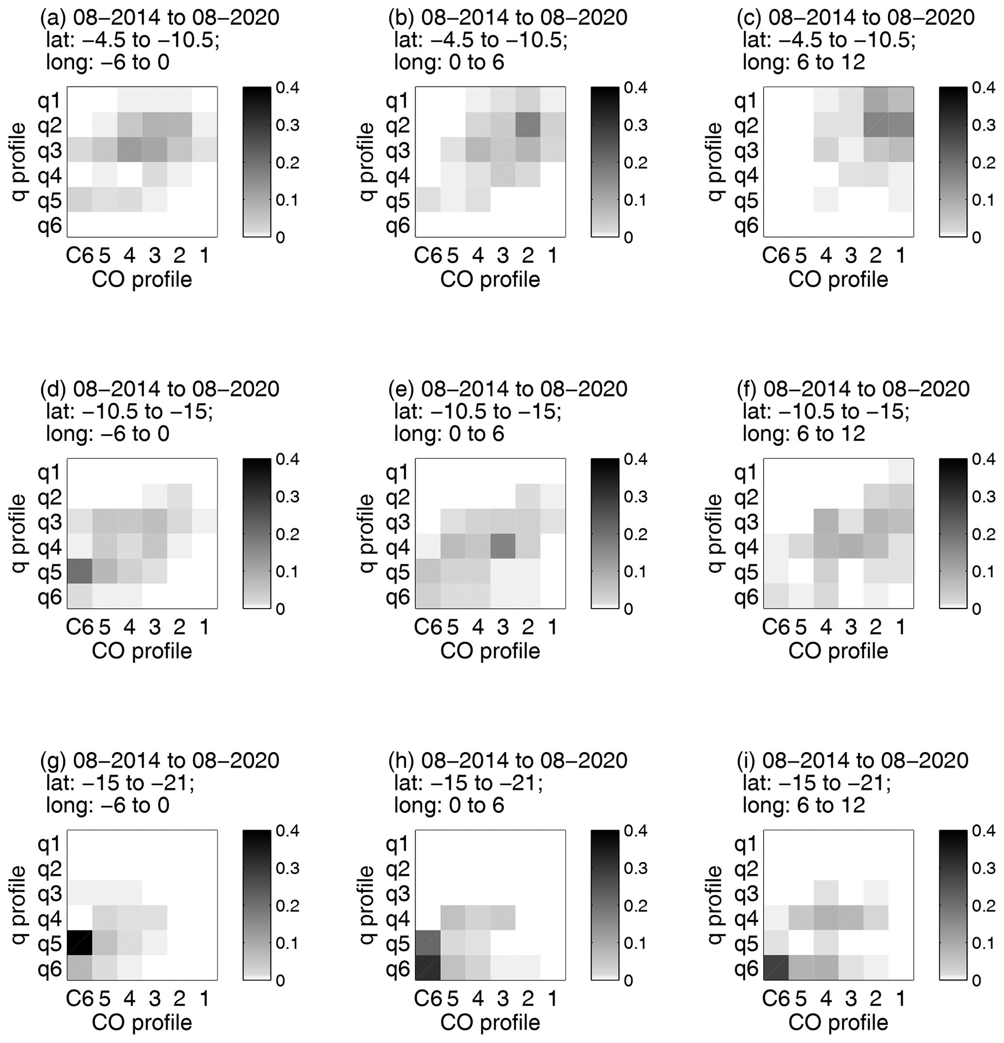
Figure 10The k-means classifications of q vs. CO for August. The profiles are ordered from left to right, clearest to smokiest, and from bottom to top, driest to most humid, and are standardized to show the fractional incidence of each profile in the same shading scale for each region. As described in the text, the spatial patterns of the smoke and humidity profiles are evident.
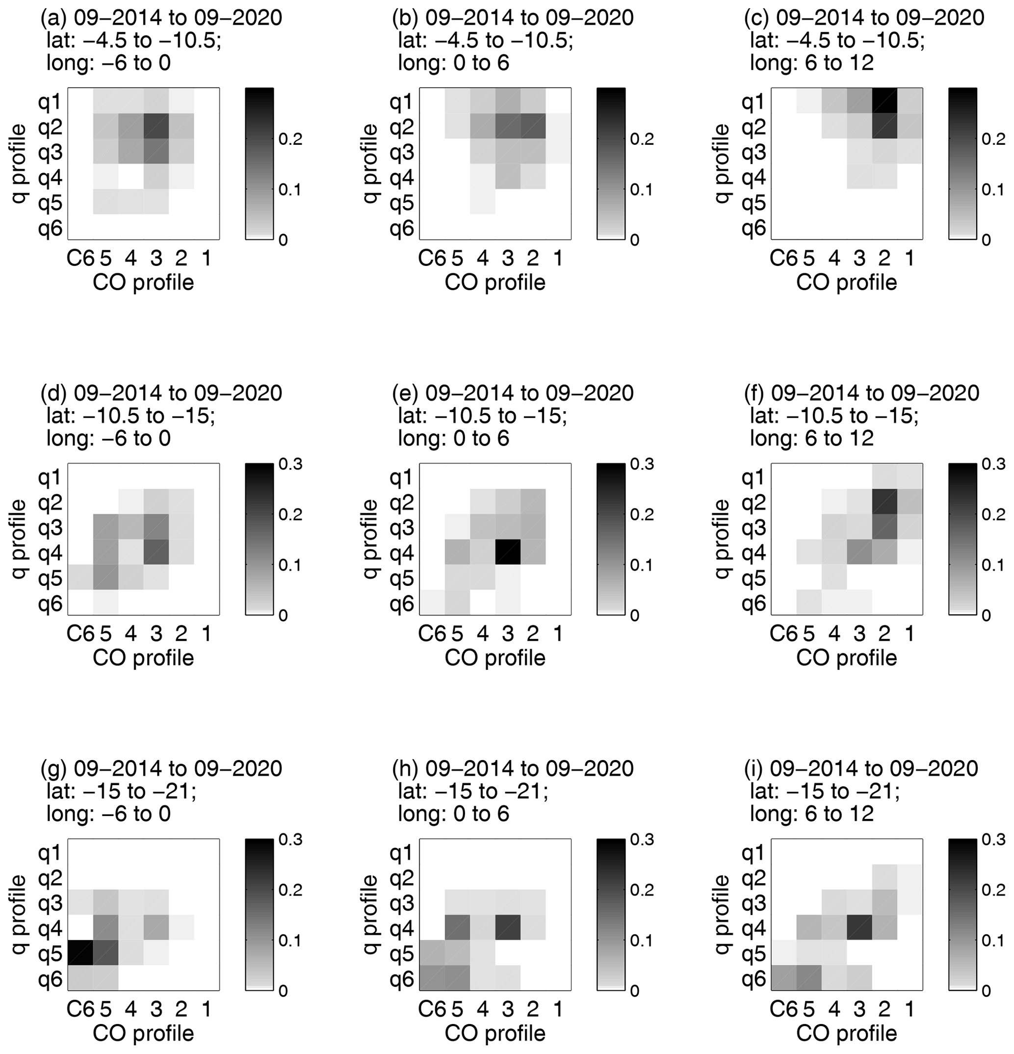

Viewing the SEA atmospheric structure in this way gives us 36 different potential smoke/water vapor combined structures, but fortunately there are fewer in reality. Figures 10, 11, and 12 show the frequency of CO–q profile combinations for each month divided into the same latitude/longitude sectors. Again, profiles are ordered from nominally least to most CO and q on their respective axes. The results are consistent with those shown in Sect. 3 using data from the ORACLES flights: while there is a range of combinations in all months, the highest frequency combinations fall along the low–low/high–high continuum. The patterns of Figs. 7 and 8 hold as well: the southernmost zones have the greatest incidence of clean and dry profiles from the southwest. The high–high conditions (q2/C2) are seen to be most frequent mid-season in September, and the latitudes of the AEJ-S have the greatest CO and vapor, decreasing with distance from the coast and with time.
There is a good deal of spatial and temporal variation to how these profiles covary. For example, in August (Fig. 10), moving from east to west along the northernmost sectors (following the AEJ-S outflow), there is a relatively disperse range of conditions that are generally high-q, high-CO combinations at around 10 % each (i.e., medium/high: q2/[C3,C4], q3/[C2,C3,C4]), although the q2/C2 condition is still a frequent combination especially nearest to the coast (∼ 20 %). In the middle latitudes, conditions become progressively more distributed along the high–high/low–low continuum, q5/C5, q4/C5, and q4/C4, again on the order of 10 % each. The maximum frequencies in this range are q5/C6 (with a maximum of 24 % farthest from coast) and q4/C3 (21 % middle longitudes). To the south, the low-CO, low-q conditions (q5/C6, q6/C6) dominate more significantly (a combined 70 %, 59 %, and 33 % moving west to east), although episodes of smoky air still occur (27 % C4 nearest to the coast) under a range of humidity conditions (for C4, the conditions are fairly evenly split between q4 and q6).
In September (Fig. 11), the profiles more strongly favor a more frequent incidence of fewer combinations in all regions (e.g., q1/C2 and q2/C2 comprise 56 % of cases in the northeast, and q5/C6 and q5/C5 comprise 51 % of cases in the southwest). By October (Fig. 12), when the highest CO (C1) profiles are almost entirely absent, the most common northeastern coastal profile is high humidity, medium–low CO (i.e., q1/[C2,C3,C4] at [39 %, 12 %, 12 %] for a total of 64 % of cases in this range), consistent with the aircraft observations. A good example of the seasonal progression is in the middle-easternmost box, which shows a range of combinations in all months, but progresses from skewed high-CO, low-q (i.e., q5/C1, q6/C4) in August to high-q, low-CO (q4/C5, q2/C4) in October, with around 10 % incidence of each. This presentation also highlights how smokeless conditions are rarely seen after August at the northern AEJ-S latitudes, despite lower smoke emissions in October. We also see an evolution of the overall variability in conditions, with some sectors (e.g., September/October in the south) showing more variability in q than in CO, while others show more variability in CO than in q (e.g., August in middle latitudes or October in the northern latitudes). We also note that while clear diurnal cycles in temperature, potential temperature, humidity, and CO are evident in the reanalysis over land, these effects are muted once the air is transported over the ocean regions, and there are no significant changes in profile class across the diurnal cycle. The major variations in atmospheric structure seen here are spatial and seasonal and may reflect the episodic nature of smoke transport across the AEJ-S (e.g., Ryoo et al., 2021; Pistone et al., 2021). While a bit daunting, this large range of conditions within a limited spatial area offers an ideal framework in which to quantify the radiative impacts of vapor, aerosol, and their various combinations.
Our work thus far has provided a descriptive characterization for the smoke–vapor relationship, both from targeted aircraft-based field measurements and in a larger reanalysis-based context. In this section, we aim to place this characterization into the broader analysis context, so as to describe its relevance to other studies and to motivate future work utilizing the results presented here.
Several previous studies highlighted the importance of examining the aerosol–water vapor covariance over this SEA region, and this work is relevant to those results. As was discussed earlier, Adebiyi et al. (2015) used a few idealized case studies (low, medium, and high AOD) based on satellite and radiosonde data at St Helena (15.9° S, 5.6° W) to estimate a maximum increase in shortwave heating due to moisture of 0.12 K d−1 compared with 1.2 K d−1 of aerosol SW heating. In the longwave, they found the presence of moisture resulted in a maximum net cooling of 0.45 K d−1 at the top of the moisture layer, with a consequent reduction in radiation passing through the humid layer into the boundary layer. Within the context of this current study, we expect these conditions, which fall into the southwest grid box of our framework (Fig. 1d), to reflect only a small amount of the total radiative forcing, given the higher plume concentrations which are more frequent elsewhere over the SEA.
Deaconu et al. (2019) similarly noted the water vapor and aerosol covariance in their study using POLDER, MODIS, CALIPSO, and ERA-Interim, but this study focused on the less humid June–August time frame and specifically was interested in the impacts of this layer on underlying clouds. They found roughly 6 K d−1 aerosol warming at the aerosol layer for defined high- vs. low-aerosol cases and a corresponding water vapor effect of 0.76 K d−1 SW (warming) and −0.14 K d−1 LW (cooling). We note that both this work and that of Adebiyi et al. (2015) chose a framework of essentially “low” or “high” aerosol rather than a more discretized classification or one that considers the varying vertical structure of the atmosphere over this region.
A more targeted study was performed by Cochrane et al. (2022), who used high-vertical-resolution aircraft data to quantify the aerosol and water vapor heading rates for specific case studies from flights in ORACLES-2016 and ORACLES-2017. The authors found that for the cases examined, the average maximum aerosol heating rate was 4.6 K d−1 and that of water vapor was 2.8 K d−1 or ∼ 60 % of the aerosol value and 4–10 times greater than the water vapor heating of the other studies. The cases considered in Cochrane et al. (2022) are noted to have had much higher aerosol loading (AODs typically exceeding 0.4, compared to the > 0.2 threshold used by Adebiyi et al., 2015). The localized nature of each of these previous results highlights the importance of being able to accurately characterize atmospheric conditions over different parts of a given region. We also note that the case studies of Cochrane et al. (2022) are included in the profile-based analysis we present here (specifically, distributed across the middle/coastal longitude ranges north of 15° S and in the southeast zone south of 15° S), which will allow us to directly assess the agreement between the approaches.
Another recent study from Johnson and Haywood (2023) calculated that BC absorption in models facilitated self-lofting (increase in buoyancy due to aerosol heating), which has various potentially significant impacts on atmospheric dynamics and aerosol lifetime. Over the SEA, they calculated an additional lofting of 0.5 km, which may be significant given the consistent subsidence in the region, delaying the eventual mixing into the underlying cloud deck. Finally, a recent study from Baró Pérez et al. (2024) used large eddy simulations initialized by ORACLES-2017 observations to isolate and quantify the effects of the humid smoke plume on the underlying cloud fields. They concluded that the presence of moisture in the plume overlying the stratocumulus clouds produced a cooling effect of roughly the same magnitude as the total aerosol effect in these cases, highlighting the importance of humidity on the clouds and climate in this region.
Here, we have utilized observational datasets to describe the atmospheric structure of the SEA during the springtime BB season and to assess how well the unique vertical features of the region are captured in several frequently used reanalyses. Using different elements of the comprehensive ORACLES airborne dataset, we conclude that the ECMWF reanalyses offer a fairly accurate characterization throughout the season August–October and that the vertical structure of the CO tracer is a reasonable proxy for aerosol optical effects. These results are important because the radiative conditions vary over the region and with the season. The radiative heating of a given atmospheric layer strongly depends on the local insolation/solar zenith angle (e.g., Cochrane et al., 2022), which varies spatially and seasonally. Additionally, by characterizing the spatial (specifically longitudinal) variation of conditions in the region, we may be able to gain a better understanding of the lifetime influence of a particular air mass, i.e., the temporal extent of its radiative influence on the atmosphere/cloud column. This framework allows us to characterize the conditions in a more digestible format and to construct a more realistic atmospheric frequency distribution. The results of this study can aid in performing radiative transfer calculations in the regions of plume maximum, allowing us to put both isolated aircraft-based case studies and analysis of surface-based measurement sites into a broader context. This will be the subject of future work. Overall, the large range of conditions seen here, validated by the ORACLES aircraft measurements, offers an intriguing opportunity to explore the differing radiative impacts of water vapor in conjunction with a radiatively active BB plume.
Here, we have explored various aspects of the observed BB layer and coincident elevated humidity signal over the SEA. We show the observed CO–q relationship is consistent across three field deployments over the BB season, although the magnitude of the relationship varies (slopes of 0.020, 0.023, and 0.05 (g kg−1) ppb−1 for August 2017, September 2016, and October 2018, respectively) due to changing meteorological and BB conditions as the season progresses. Despite the differing locations and timing of each deployment, we have shown that good agreement between the airborne ORACLES dataset and large-scale reanalyses is consistent across the deployments, specifically for the ECMWF ERA5 and CAMS reanalyses.
Consistent with the results of Pistone et al. (2021) for September 2016, the ERA5 reanalysis of water vapor agrees well with the ORACLES observations (R2=0.78, 0.90, and 0.89 for September 2016, August 2017, and October 2018, respectively). The CAMS reanalysis also agrees well with observed water vapor (R2=0.84, 0.85, and 0.92 for September 2016, August 2017, and October 2018, respectively), albeit with lower resolution than the ERA5 reanalysis. CAMS represents water vapor somewhat more realistically than it does CO (campaign-wide R2=0.74, 0.73, and 0.54 for September 2016, August 2017, and October 2018), with CO tending to be underestimated relative to observations especially under high smoke concentrations. By contrast, CAMS column aerosol optical depth (AOD) shows similar correlations to those of CO, but the CAMS AOD values are generally overestimated relative to the field measurements. While NASA's MERRA-2 reanalysis preserves the observed correlation between CO and q, the smoky air masses are frequently displaced (too low in altitude) in MERRA-2 relative to the observations, resulting in poorer direct correlations between MERRA-2 and the observations. This is consistent with the results of Pistone et al. (2021), which focused on the September 2016 observations. Nonetheless, inlet-based observations show a consistent relationship between CO and aerosol extinction across all observations, demonstrating the utility of the CO tracer to understanding vertical aerosol distribution across the season.
Following this good agreement between ORACLES and CAMS/ERA5, we next presented a k-means clustering method using 7 years of the reanalyses (August–October 2014–2020) to examine the multi-year seasonal patterns and trends. While the humidity profiles are distinguished by both variations in total humidity and vertical structure, the CO profiles show a more uniform range, being primarily distinguished by maximum concentration in the free troposphere. Spatially and temporally, we see consistent spatial and temporal variations in smoke and humidity distribution (total concentration and vertical structure) and their correlations to one another, reflecting changing conditions through the BB season. Generally, the high-humidity, high-CO profiles dominate in August and September in the northeast of the study region, and high-humidity, medium-CO dominates in October, with consistently lower concentrations in the southwest of the region. There, the atmosphere is largely unaffected by the smoke transported in the AEJ-S in August, although by October the entire region considered (6° W–12° E, 5–21° S) is influenced by smoke and humidity to some degree. The distributions of the covaried q/CO profiles range from being fairly strongly dominated by one type (30 %–40 % for a given CO/q combination) to more evenly distributed between many profile types (∼ 5 %–10 % per type) in different places and times or indeed in the same places at different times, highlighting the variation in episodic transport over this region.
With this work, we have established a framework which allows us to more completely understand the spatial and temporal variations over the SEA, not just in atmospheric structure of water vapor and chemical species, but also ultimately of the radiative effects of the elevated water vapor signal working in concert with the absorbing aerosol biomass burning plume. By establishing the consistently good agreement between the ERA5 and CAMS reanalyses and the aircraft observations, we can use the reanalyses to describe the frequency of conditions over the SEA. The six k-means profiles each for CO and q allow for a comprehensive range of conditions to be described, while still limiting the total number of permutations to a manageable number. Previous studies have demonstrated the importance of water vapor and BB heating in this region, and in further work will use this framework to comprehensively assess the impacts of the vertical and spatial structural variance of this region. The range in profile types, even as the general high-smoke, high-humidity pattern remains, will allow us to quantify the radiative effects of atmospheric humidity and aerosol in this region, both together and as separate components. These results have potential impacts on our understanding of general circulation in the region, large-scale subsidence, precipitation distribution, and mixing of BB into the cloud-topped boundary layer. Overall, this will allow for a more complete and nuanced assessment of the aerosol–radiation–climate interactions in this region.
The flight data used in this paper are publicly available at https://doi.org/10.5067/Suborbital/ORACLES/P3/2016_V1 (ORACLES Science Team, 2017), https://doi.org/10.5067/Suborbital/ORACLES/P3/2017_V1 (ORACLES Science Team, 2019a), and https://doi.org/10.5067/Suborbital/ORACLES/P3/2018_V1 (ORACLES Science Team, 2019b) for the 2016, 2017, and 2018 data, respectively. The codes used in processing 4STAR data may be found at https://doi.org/10.5281/zenodo.1492912 (4STAR Team et al., 2018). ECMWF reanalyses are available at the Copernicus Climate Data Store (https://doi.org/10.24381/cds.143582cf, Hersbach et al., 2017) or the Atmospheric Data Store (https://ads.atmosphere.copernicus.eu/cdsapp#!/dataset/cams-global-reanalysis-eac4, Inness et al., 2019) for ERA5 and CAMS, respectively, subset and ordered according to the parameters described in the text. The MERRA-2 products used are available online at https://portal.nccs.nasa.gov/datashare/iesa/campaigns/ORACLES/ (Collow et al., 2020).
The supplement related to this article is available online at: https://doi.org/10.5194/acp-24-7983-2024-supplement.
KP designed the research, performed the ORACLES/reanalysis comparisons, and produced the figures. EMW processed the ERA5 and CAMS reanalyses to provide the k-means cluster results, methodology, analysis, and relevant supplementary figures. COMA data were collected and processed by JP. 4STAR data were collected and processed by SEL, KP, and MK. HiGEAR data were collected and processed by SGH and SF. KP wrote the paper in discussion with EMW and PZ; all other coauthors had the opportunity to provide feedback on the methods, manuscript, and results.
The contact author has declared that none of the authors has any competing interests.
Publisher's note: Copernicus Publications remains neutral with regard to jurisdictional claims made in the text, published maps, institutional affiliations, or any other geographical representation in this paper. While Copernicus Publications makes every effort to include appropriate place names, the final responsibility lies with the authors.
This article is part of the special issue “New observations and related modelling studies of the aerosol–cloud–climate system in the Southeast Atlantic and southern Africa regions (ACP/AMT inter-journal SI)”. It is not associated with a conference.
Kristina Pistone, Eric M. Wilcox, and Marco Giordano's time was funded by NASA ACCDAM grant 20-ACCDAM20-0087. The ORACLES mission was funded by NASA Earth Venture Suborbital-2 grant NNH13ZDA001N-EVS2. Like most field work, the ORACLES project was very much a team effort; we thank the ORACLES deployment support teams, the ORACLES science team (for a more complete accounting, see the author list and Table C1 in Redemann et al., 2021), and the governments and people of Walvis Bay and Swakopmund, Namibia, and of São Tomé, São Tomé and Príncipe, for a successful and productive mission. We thank Ju-Mee Ryoo for many helpful conversations and comments and Stephen Broccardo for comments on earlier drafts of this work.
This research has been supported by the National Aeronautics and Space Administration (grant no. 20-ACCDAM20-0087, NNH13ZDA001N-EVS2).
This paper was edited by N'Datchoh Evelyne Touré and reviewed by two anonymous referees.
4STAR Team, LeBlanc, S., Flynn, C. J., Shinozuka, Y., Segal-Rozenhaimer, M., Pistone, K., Kacenelenbogen, M., Redemann, J., Schmid, B., Russell, P., Livingston, J., and Zhang, Q.: 4STAR_codes: 4STAR processing codes (v1.0.1), Zenodo [code], https://doi.org/10.5281/zenodo.1492912, 2018. a
Ackerman, A. S., Kirkpatrick, M. P., Stevens, D. E., and Toon, O. B.: The impact of humidity above stratiform clouds on indirect aerosol climate forcing, Nature, 432, 1014–1017, https://doi.org/10.1038/nature03174, 2004. a
Adebiyi, A. A. and Zuidema, P.: The role of the southern African easterly jet in modifying the southeast Atlantic aerosol and cloud environments, Q. J. Roy. Meteor. Soc., 142, 1574–1589, https://doi.org/10.1002/qj.2765, 2016. a
Adebiyi, A. A., Zuidema, P., and Abel, S. J.: The Convolution of Dynamics and Moisture with the Presence of Shortwave Absorbing Aerosols over the Southeast Atlantic, J. Climate, 28, 1997–2024, https://doi.org/10.1175/JCLI-D-14-00352.1, 2015. a, b, c, d, e, f
Anderson, T. and Ogren, J.: Determining aerosol radiative properties using the TSI 3563 integrating nephelometer, Aerosol Sci. Tech., 29, 57–69, https://doi.org/10.1080/02786829808965551, 1998. a
Anderson, T., Masonis, S., Covert, D., Ahlquist, N., Howell, S., Clarke, A., and McNaughton, C.: Variability of aerosol optical properties derived from in situ aircraft measurements during ACE-Asia, J. Geophys. Res.-Atmos., 108, 8647, https://doi.org/10.1029/2002JD003247, 2003. a
Baró Pérez, A., Diamond, M. S., Bender, F. A.-M., Devasthale, A., Schwarz, M., Savre, J., Tonttila, J., Kokkola, H., Lee, H., Painemal, D., and Ekman, A. M. L.: Comparing the simulated influence of biomass burning plumes on low-level clouds over the southeastern Atlantic under varying smoke conditions, Atmos. Chem. Phys., 24, 4591–4610, https://doi.org/10.5194/acp-24-4591-2024, 2024. a, b
Buchard, V., Randles, C. A., da Silva, A. M., Darmenov, A., Colarco, P. R., Govindaraju, R., Ferrare, R., Hair, J., Beyersdorf, A. J., Ziemba, L. D., and Yu, H.: The MERRA-2 Aerosol Reanalysis, 1980 Onward. Part II: Evaluation and Case Studies, J. Climate, 30, 6851–6872, https://doi.org/10.1175/JCLI-D-16-0613.1, 2017. a
Chang, I., Gao, L., Burton, S. P., Chen, H., Diamond, M. S., Ferrare, R. A., Flynn, C. J., Kacenelenbogen, M., LeBlanc, S. E., Meyer, K. G., Pistone, K., Schmidt, S., Segal-Rozenhaimer, M., Shinozuka, Y., Wood, R., Zuidema, P., Redemann, J., and Christopher, S. A.: Spatiotemporal Heterogeneity of Aerosol and Cloud Properties Over the Southeast Atlantic: An Observational Analysis, Geophys. Res. Lett., 48, e2020GL091469, https://doi.org/10.1029/2020GL091469 2021. a
Che, H., Segal-Rozenhaimer, M., Zhang, L., Dang, C., Zuidema, P., Sedlacek III, A. J., Zhang, X., and Flynn, C.: Seasonal variations in fire conditions are important drivers in the trend of aerosol optical properties over the south-eastern Atlantic, Atmos. Chem. Phys., 22, 8767–8785, https://doi.org/10.5194/acp-22-8767-2022, 2022. a
Cochrane, S. P., Schmidt, K. S., Chen, H., Pilewskie, P., Kittelman, S., Redemann, J., LeBlanc, S., Pistone, K., Segal Rozenhaimer, M., Kacenelenbogen, M., Shinozuka, Y., Flynn, C., Ferrare, R., Burton, S., Hostetler, C., Mallet, M., and Zuidema, P.: Biomass burning aerosol heating rates from the ORACLES (ObseRvations of Aerosols above CLouds and their intEractionS) 2016 and 2017 experiments, Atmos. Meas. Tech., 15, 61–77, https://doi.org/10.5194/amt-15-61-2022, 2022. a, b, c, d, e, f
Collow, A., Lucchesi, R., and Da Silva, A.: File Specification for GEOS Products Sampled Along Aircraft Trajectories, Tech. Rep. Office Note No. 18 (Version 1.0), GMAO, http://gmao.gsfc.nasa.gov/pubs/office_notes (last access: 21 June 2021), 2020. a, b
Das, S., Harshvardhan, H., Bian, H., Chin, M., Curci, G., Protonotariou, A. P., Mielonen, T., Zhang, K., Wang, H., and Liu, X.: Biomass burning aerosol transport and vertical distribution over the South African-Atlantic region, J. Geophys. Res.-Atmos., 122, 6391–6415, https://doi.org/10.1002/2016JD026421, 2017. a
Deaconu, L. T., Ferlay, N., Waquet, F., Peers, F., Thieuleux, F., and Goloub, P.: Satellite inference of water vapour and above-cloud aerosol combined effect on radiative budget and cloud-top processes in the southeastern Atlantic Ocean, Atmos. Chem. Phys., 19, 11613–11634, https://doi.org/10.5194/acp-19-11613-2019, 2019. a, b
Doherty, S. J., Saide, P. E., Zuidema, P., Shinozuka, Y., Ferrada, G. A., Gordon, H., Mallet, M., Meyer, K., Painemal, D., Howell, S. G., Freitag, S., Dobracki, A., Podolske, J. R., Burton, S. P., Ferrare, R. A., Howes, C., Nabat, P., Carmichael, G. R., da Silva, A., Pistone, K., Chang, I., Gao, L., Wood, R., and Redemann, J.: Modeled and observed properties related to the direct aerosol radiative effect of biomass burning aerosol over the southeastern Atlantic, Atmos. Chem. Phys., 22, 1–46, https://doi.org/10.5194/acp-22-1-2022, 2022. a
Dunagan, S. E., Johnson, R., Zavaleta, J., Russell, P. B., Schmid, B., Flynn, C., Redemann, J., Shinozuka, Y., Livingston, J., and Segal-Rosenhaimer, M.: Spectrometer for Sky-Scanning Sun-Tracking Atmospheric Research (4STAR): Instrument Technology, Remote Sens., 5, 3872–3895, https://doi.org/10.3390/rs5083872, 2013. a
Eck, T. F., Holben, B. N., Reid, J. S., Mukelabai, M. M., Piketh, S. J., Torres, O., Jethva, H. T., Hyer, E. J., Ward, D. E., Dubovik, O., Sinyuk, A., Schafer, J. S., Giles, D. M., Sorokin, M., Smirnov, A., and Slutsker, I.: A seasonal trend of single scattering albedo in southern African biomass-burning particles: Implications for satellite products and estimates of emissions for the world's largest biomass-burning source, J. Geophys. Res.-Atmos., 118, 6414–6432, https://doi.org/10.1002/jgrd.50500, 2013. a
Forster, P., Storelvmo, T., Armour, K., Collins, W., Dufresne, J.-L., Frame, D., Lunt, D., Mauritsen, T., Palmer, M., Watanabe, M., Wild, M., and Zhang, H.: The Earth's Energy Budget, Climate Feedbacks, and Climate Sensitivity, book section 7, in: Climate Change 2021: The Physical Science Basis. Contribution of Working Group I to the Sixth Assessment Report of the Intergovernmental Panel on Climate Change, edited by: Masson-Delmotte, V., Zhai, P., Pirani, A., Connors, S. L., Péan, C., Berger, S., Caud, N., Chen, Y., Goldfarb, L., Gomis, M. I., Huang, M., Leitzell, K., Lonnoy, E., Matthews, J. B. R., Maycock, T. K., Waterfield, T., Yelekçi, O., Yu, R., and Zhou, B., Cambridge University Press, Cambridge, United Kingdom and New York, NY, USA, 923–1054, https://doi.org/10.1017/9781009157896.009, 2021. a
Gelaro, R., McCarty, W., Suárez, M. J., Todling, R., Molod, A., Takacs, L., Randles, C. A., Darmenov, A., Bosilovich, M. G., Reichle, R., Wargan, K., Coy, L., Cullather, R., Draper, C., Akella, S., Buchard, V., Conaty, A., da Silva, A. M., Gu, W., Kim, G.-K., Koster, R., Lucchesi, R., Merkova, D., Nielsen, J. E., Partyka, G., Pawson, S., Putman, W., Rienecker, M., Schubert, S. D., Sienkiewicz, M., and Zhao, B.: The Modern-Era Retrospective Analysis for Research and Applications, Version 2 (MERRA-2), J. Climate, 30, 5419–5454, https://doi.org/10.1175/JCLI-D-16-0758.1, 2017. a
Haywood, J., Francis, P., Dubovik, O., Glew, M., and Holben, B.: Comparison of aerosol size distributions, radiative properties, and optical depths determined by aircraft observations and Sun photometers during SAFARI 2000, J. Geophys. Res.-Atmos., 108, 8471, https://doi.org/10.1029/2002JD002250, 2003. a
Hersbach, H., Bell, B., Berrisford, P., Hirahara, S., Horányi, A., Muñoz‐Sabater, J., Nicolas, J., Peubey, C., Radu, R., Schepers, D., Simmons, A., Soci, C., Abdalla, S., Abellan, X., Balsamo, G., Bechtold, P., Biavati, G., Bidlot, J., Bonavita, M., De Chiara, G., Dahlgren, P., Dee, D., Diamantakis, M., Dragani, R., Flemming, J., Forbes, R., Fuentes, M., Geer, A., Haimberger, L., Healy, S., Hogan, R. J., Hólm, E., Janisková, M., Keeley, S., Laloyaux, P., Lopez, P., Lupu, C., Radnoti, G., de Rosnay, P., Rozum, I., Vamborg, F., Villaume, S., and Thépaut, J.-N.: Complete ERA5 from 1940: Fifth generation of ECMWF atmospheric reanalyses of the global climate, Copernicus Climate Change Service (C3S) Data Store (CDS) [data set], https://doi.org/10.24381/cds.143582cf, 2017. a
Hersbach, H., Bell, B., Berrisford, P., Hirahara, S., Horányi, A., Muñoz-Sabater, J., Nicolas, J., Peubey, C., Radu, R., Schepers, D., Simmons, A., Soci, C., Abdalla, S., Abellan, X., Balsamo, G., Bechtold, P., Biavati, G., Bidlot, J., Bonavita, M., De Chiara, G., Dahlgren, P., Dee, D., Diamantakis, M., Dragani, R., Flemming, J., Forbes, R., Fuentes, M., Geer, A., Haimberger, L., Healy, S., Hogan, R. J., Hólm, E., Janisková, M., Keeley, S., Laloyaux, P., Lopez, P., Lupu, C., Radnoti, G., de Rosnay, P., Rozum, I., Vamborg, F., Villaume, S., and Thépaut, J.-N.: The ERA5 global reanalysis, Q. J. Roy. Meteor. Soc., 146, 1999–2049, https://doi.org/10.1002/qj.3803, 2020. a, b
Inness, A., Ades, M., Agustí-Panareda, A., Barré, J., Benedictow, A., Blechschmidt, A.-M., Dominguez, J. J., Engelen, R., Eskes, H., Flemming, J., Huijnen, V., Jones, L., Kipling, Z., Massart, S., Parrington, M., Peuch, V.-H., Razinger, M., Remy, S., Schulz, M., and Suttie, M.: The CAMS reanalysis of atmospheric composition, Atmos. Chem. Phys., 19, 3515–3556, https://doi.org/10.5194/acp-19-3515-2019, 2019 (data available at: https://ads.atmosphere.copernicus.eu/cdsapp#!/dataset/cams-global-reanalysis-eac4, last access: 31 August 2021). a, b, c, d, e, f, g, h
Inness, A., Aben, I., Ades, M., Borsdorff, T., Flemming, J., Jones, L., Landgraf, J., Langerock, B., Nedelec, P., Parrington, M., and Ribas, R.: Assimilation of S5P/TROPOMI carbon monoxide data with the global CAMS near-real-time system, Atmos. Chem. Phys., 22, 14355–14376, https://doi.org/10.5194/acp-22-14355-2022, 2022. a, b
Johnson, B. T. and Haywood, J. M.: Assessing the Impact of Self-Lofting on Increasing the Altitude of Black Carbon in a Global Climate Model, J. Geophys. Res.-Atmos., 128, e2022JD038039, https://doi.org/10.1029/2022JD038039, 2023. a
Koch, D. and Del Genio, A. D.: Black carbon semi-direct effects on cloud cover: review and synthesis, Atmos. Chem. Phys., 10, 7685–7696, https://doi.org/10.5194/acp-10-7685-2010, 2010. a
LeBlanc, S. E., Redemann, J., Flynn, C., Pistone, K., Kacenelenbogen, M., Segal-Rosenheimer, M., Shinozuka, Y., Dunagan, S., Dahlgren, R. P., Meyer, K., Podolske, J., Howell, S. G., Freitag, S., Small-Griswold, J., Holben, B., Diamond, M., Wood, R., Formenti, P., Piketh, S., Maggs-Kölling, G., Gerber, M., and Namwoonde, A.: Above-cloud aerosol optical depth from airborne observations in the southeast Atlantic, Atmos. Chem. Phys., 20, 1565–1590, https://doi.org/10.5194/acp-20-1565-2020, 2020. a, b, c
Liu, X., Huey, L. G., Yokelson, R. J., Selimovic, V., Simpson, I. J., Müller, M., Jimenez, J. L., Campuzano-Jost, P., Beyersdorf, A. J., Blake, D. R., Butterfield, Z., Choi, Y., Crounse, J. D., Day, D. A., Diskin, G. S., Dubey, M. K., Fortner, E., Hanisco, T. F., Hu, W., King, L. E., Kleinman, L., Meinardi, S., Mikoviny, T., Onasch, T. B., Palm, B. B., Peischl, J., Pollack, I. B., Ryerson, T. B., Sachse, G. W., Sedlacek, A. J., Shilling, J. E., Springston, S., St. Clair, J. M., Tanner, D. J., Teng, A. P., Wennberg, P. O., Wisthaler, A., and Wolfe, G. M.: Airborne measurements of western U.S. wildfire emissions: Comparison with prescribed burning and air quality implications, J. Geophys. Res.-Atmos., 122, 6108–6129, https://doi.org/10.1002/2016JD026315, 2017. a
Magi, B. and Hobbs, P.: Effects of humidity on aerosols in southern Africa during the biomass burning season, J. Geophys. Res.-Atmos., 108, 8495, https://doi.org/10.1029/2002JD002144, 2003. a
McNaughton, C. S., Clarke, A. D., Freitag, S., Kapustin, V. N., Kondo, Y., Moteki, N., Sahu, L., Takegawa, N., Schwarz, J. P., Spackman, J. R., Watts, L., Diskin, G., Podolske, J., Holloway, J. S., Wisthaler, A., Mikoviny, T., de Gouw, J., Warneke, C., Jimenez, J., Cubison, M., Howell, S. G., Middlebrook, A., Bahreini, R., Anderson, B. E., Winstead, E., Thornhill, K. L., Lack, D., Cozic, J., and Brock, C. A.: Absorbing aerosol in the troposphere of the Western Arctic during the 2008 ARCTAS/ARCPAC airborne field campaigns, Atmos. Chem. Phys., 11, 7561–7582, https://doi.org/10.5194/acp-11-7561-2011, 2011. a
Morcrette, J.-J., Boucher, O., Jones, L., Salmond, D., Bechtold, P., Beljaars, A., Benedetti, A., Bonet, A., Kaiser, J. W., Razinger, M., Schulz, M., Serrar, S., Simmons, A. J., Sofiev, M., Suttie, M., Tompkins, A. M., and Untch, A.: Aerosol analysis and forecast in the European Centre for Medium-Range Weather Forecasts Integrated Forecast System: Forward modeling, J. Geophys. Res.-Atmos., 114, D06206, https://doi.org/10.1029/2008JD011235, 2009. a
ORACLES Science Team: Suite of Aerosol, Cloud, and Related Data Acquired Aboard P3 During ORACLES 2016, Version 1, NASA Ames Earth Science Project Office (ESPO), Moffett Field, CA [data set], https://doi.org/10.5067/Suborbital/ORACLES/P3/2016_V1, 2017. a
ORACLES Science Team: Suite of Aerosol, Cloud, and Related Data Acquired Aboard P3 During ORACLES 2017, Version 1, NASA Ames Earth Science Project Office (ESPO), Moffett Field, CA [data set], https://doi.org/10.5067/Suborbital/ORACLES/P3/2017_V1, 2019a. a
ORACLES Science Team: Suite of Aerosol, Cloud, and Related Data Acquired Aboard P3 During ORACLES 2018, Version 1, NASA Ames Earth Science Project Office (ESPO), Moffett Field, CA [data set], https://doi.org/10.5067/Suborbital/ORACLES/P3/2018_V1, 2019b. a
Pistone, K., Redemann, J., Doherty, S., Zuidema, P., Burton, S., Cairns, B., Cochrane, S., Ferrare, R., Flynn, C., Freitag, S., Howell, S. G., Kacenelenbogen, M., LeBlanc, S., Liu, X., Schmidt, K. S., Sedlacek III, A. J., Segal-Rozenhaimer, M., Shinozuka, Y., Stamnes, S., van Diedenhoven, B., Van Harten, G., and Xu, F.: Intercomparison of biomass burning aerosol optical properties from in situ and remote-sensing instruments in ORACLES-2016, Atmos. Chem. Phys., 19, 9181–9208, https://doi.org/10.5194/acp-19-9181-2019, 2019. a, b
Pistone, K., Zuidema, P., Wood, R., Diamond, M., da Silva, A. M., Ferrada, G., Saide, P. E., Ueyama, R., Ryoo, J.-M., Pfister, L., Podolske, J., Noone, D., Bennett, R., Stith, E., Carmichael, G., Redemann, J., Flynn, C., LeBlanc, S., Segal-Rozenhaimer, M., and Shinozuka, Y.: Exploring the elevated water vapor signal associated with the free tropospheric biomass burning plume over the southeast Atlantic Ocean, Atmos. Chem. Phys., 21, 9643–9668, https://doi.org/10.5194/acp-21-9643-2021, 2021. a, b, c, d, e, f, g, h, i, j, k, l, m, n, o, p, q, r
Provencal, R., Gupta, M., Owano, T. G., Baer, D. S., Ricci, K. N., O'Keefe, A., and Podolske, J. R.: Cavity-enhanced quantum-cascade laser-based instrument for carbon monoxide measurements, Appl. Opt., 44, 6712–6717, https://doi.org/10.1364/AO.44.006712, 2005. a
Randles, C. A., da Silva, A. M., Buchard, V., Colarco, P. R., Darmenov, A., Govindaraju, R., Smirnov, A., Holben, B., Ferrare, R., Hair, J., Shinozuka, Y., and Flynn, C. J.: The MERRA-2 Aerosol Reanalysis, 1980 Onward. Part I: System Description and Data Assimilation Evaluation, J. Climate, 30, 6823–6850, https://doi.org/10.1175/JCLI-D-16-0609.1, 2017. a
Redemann, J., Wood, R., Zuidema, P., Doherty, S. J., Luna, B., LeBlanc, S. E., Diamond, M. S., Shinozuka, Y., Chang, I. Y., Ueyama, R., Pfister, L., Ryoo, J.-M., Dobracki, A. N., da Silva, A. M., Longo, K. M., Kacenelenbogen, M. S., Flynn, C. J., Pistone, K., Knox, N. M., Piketh, S. J., Haywood, J. M., Formenti, P., Mallet, M., Stier, P., Ackerman, A. S., Bauer, S. E., Fridlind, A. M., Carmichael, G. R., Saide, P. E., Ferrada, G. A., Howell, S. G., Freitag, S., Cairns, B., Holben, B. N., Knobelspiesse, K. D., Tanelli, S., L'Ecuyer, T. S., Dzambo, A. M., Sy, O. O., McFarquhar, G. M., Poellot, M. R., Gupta, S., O'Brien, J. R., Nenes, A., Kacarab, M., Wong, J. P. S., Small-Griswold, J. D., Thornhill, K. L., Noone, D., Podolske, J. R., Schmidt, K. S., Pilewskie, P., Chen, H., Cochrane, S. P., Sedlacek, A. J., Lang, T. J., Stith, E., Segal-Rozenhaimer, M., Ferrare, R. A., Burton, S. P., Hostetler, C. A., Diner, D. J., Seidel, F. C., Platnick, S. E., Myers, J. S., Meyer, K. G., Spangenberg, D. A., Maring, H., and Gao, L.: An overview of the ORACLES (ObseRvations of Aerosols above CLouds and their intEractionS) project: aerosol–cloud–radiation interactions in the southeast Atlantic basin, Atmos. Chem. Phys., 21, 1507–1563, https://doi.org/10.5194/acp-21-1507-2021, 2021. a, b, c, d, e
Ryoo, J.-M., Pfister, L., Ueyama, R., Zuidema, P., Wood, R., Chang, I., and Redemann, J.: A meteorological overview of the ORACLES (ObseRvations of Aerosols above CLouds and their intEractionS) campaign over the southeastern Atlantic during 2016–2018: Part 1 – Climatology, Atmos. Chem. Phys., 21, 16689–16707, https://doi.org/10.5194/acp-21-16689-2021, 2021. a, b, c, d, e
Ryoo, J.-M., Pfister, L., Ueyama, R., Zuidema, P., Wood, R., Chang, I., and Redemann, J.: A meteorological overview of the ORACLES (ObseRvations of Aerosols above CLouds and their intEractionS) campaign over the southeastern Atlantic during 2016–2018: Part 2 – Daily and synoptic characteristics, Atmos. Chem. Phys., 22, 14209–14241, https://doi.org/10.5194/acp-22-14209-2022, 2022. a, b, c
Schelbergen, M., Kalverla, P. C., Schmehl, R., and Watson, S. J.: Clustering wind profile shapes to estimate airborne wind energy production, Wind Energ. Sci., 5, 1097–1120, https://doi.org/10.5194/wes-5-1097-2020, 2020. a
Segal-Rosenheimer, M., Russell, P. B., Schmid, B., Redemann, J., Livingston, J. M., Flynn, C. J., Johnson, R. R., Dunagan, S. E., Shinozuka, Y., Herman, J., Cede, A., Abuhassan, N., Comstock, J. M., Hubbe, J. M., Zelenyuk, A., and Wilson, J.: Tracking elevated pollution layers with a newly developed hyperspectral Sun/Sky spectrometer (4STAR): Results from the TCAP 2012 and 2013 campaigns, J. Geophys. Res.-Atmos., 119, 2611–2628, https://doi.org/10.1002/2013JD020884, 2014. a
Shinozuka, Y., Saide, P. E., Ferrada, G. A., Burton, S. P., Ferrare, R., Doherty, S. J., Gordon, H., Longo, K., Mallet, M., Feng, Y., Wang, Q., Cheng, Y., Dobracki, A., Freitag, S., Howell, S. G., LeBlanc, S., Flynn, C., Segal-Rosenhaimer, M., Pistone, K., Podolske, J. R., Stith, E. J., Bennett, J. R., Carmichael, G. R., da Silva, A., Govindaraju, R., Leung, R., Zhang, Y., Pfister, L., Ryoo, J.-M., Redemann, J., Wood, R., and Zuidema, P.: Modeling the smoky troposphere of the southeast Atlantic: a comparison to ORACLES airborne observations from September of 2016, Atmos. Chem. Phys., 20, 11491–11526, https://doi.org/10.5194/acp-20-11491-2020, 2020. a, b
Shinozuka, Y., Johnson, R. R., Flynn, C. J., Russell, P. B., Schmid, B., Redemann, J., Dunagan, S. E., Kluzek, C. D., Hubbe, J. M., Segal-Rosenheimer, M., Livingston, J. M., Eck, T. F., Wagener, R., Gregory, L., Chand, D., Berg, L. K., Rogers, R. R., Ferrare, R. A., Hair, J. W., Hostetler, C. A., and Burton, S. P.: Hyperspectral aerosol optical depths from TCAP flights, J. Geophys. Res.-Atmos., 118, 12180–12194, https://doi.org/10.1002/2013JD020596, 2013. a
Szopa, S., Naik, V., Adhikary, B., Artaxo, P., Berntsen, T., Collins, W., Fuzzi, S., Gallardo, L., Kiendler-Scharr, A., Klimont, Z., Liao, H., Unger, N., and Zanis, P.: Short-Lived Climate Forcers, in: Climate Change 2021: The Physical Science Basis. Contribution of Working Group I to the Sixth Assessment Report of the Intergovernmental Panel on Climate Change, edited by: Masson-Delmotte, V., Zhai, P., Pirani, A., Connors, S. L., Péan, C., Berger, S., Caud, N., Chen, Y., Goldfarb, L., Gomis, M. I., Huang, M., Leitzell, K., Lonnoy, E., Matthews, J. B. R., Maycock, T. K., Waterfield, T., Yelekçi, O., Yu, R., and Zhou, B., Cambridge University Press, Cambridge, United Kingdom and New York, NY, USA, 817–922, https://doi.org/10.1017/9781009157896.008, 2021. a
Virkkula, A.: Correction of the Calibration of the 3-wavelength Particle Soot Absorption Photometer (3 PSAP), Aerosol Sci. Tech., 44, 706–712, https://doi.org/10.1080/02786826.2010.482110, 2010. a
Wilcox, E. M.: Stratocumulus cloud thickening beneath layers of absorbing smoke aerosol, Atmos. Chem. Phys., 10, 11769–11777, https://doi.org/10.5194/acp-10-11769-2010, 2010. a
Wilcox, E. M., Thomas, R. M., Praveen, P. S., Pistone, K., Bender, F. A.-M., and Ramanathan, V.: Black carbon solar absorption suppresses turbulence in the atmospheric boundary layer, P. Natl. Acad. Sci. USA, 113, 11794–11799, https://doi.org/10.1073/pnas.1525746113, 2016. a
Zuidema, P., Chang, P., Medeiros, B., Kirtman, B. P., Mechoso, R., Schneider, E. K., Toniazzo, T., Richter, I., Small, R. J., Bellomo, K., Brandt, P., de Szoeke, S., Farrar, J. T., Jung, E., Kato, S., Li, M., Patricola, C., Wang, Z., Wood, R., and Xu, Z.: Challenges and Prospects for Reducing Coupled Climate Model SST Biases in the Eastern Tropical Atlantic and Pacific Oceans: The U.S. CLIVAR Eastern Tropical Oceans Synthesis Working Group, B. Am. Meteorol. Soc., 97, 2305–2328, https://doi.org/10.1175/BAMS-D-15-00274.1, 2016. a
- Abstract
- Introduction
- Aircraft data and reanalyses
- Agreement between reanalyses and aircraft observations
- Spatial and temporal incidence of atmospheric vertical profiles: k-means analysis
- Discussion
- Conclusions
- Code and data availability
- Author contributions
- Competing interests
- Disclaimer
- Special issue statement
- Acknowledgements
- Financial support
- Review statement
- References
- Supplement