the Creative Commons Attribution 4.0 License.
the Creative Commons Attribution 4.0 License.
 | 19 Jan 2024
Quantifying effects of long-range transport of NO2 over Delhi using back trajectories and satellite data
Richard J. Pope
Martyn P. Chipperfield
Sandip S. Dhomse
Matilda Pimlott
Wuhu Feng
Vikas Singh
Ying Chen
Oliver Wild
Ranjeet Sokhi
Gufran Beig
Exposure to air pollution is a leading public health risk factor in India, especially over densely populated Delhi and the surrounding Indo-Gangetic Plain. During the post-monsoon seasons, the prevailing north-westerly winds are known to influence aerosol pollution events in Delhi by advecting pollutants from agricultural fires as well as from local sources. Here we investigate the year-round impact of meteorology on gaseous nitrogen oxides (). We use bottom-up NOx emission inventories (anthropogenic and fire) and high-resolution satellite measurement based tropospheric column NO2 (TCNO2) data, from S5P aboard TROPOMI, alongside a back-trajectory model (ROTRAJ) to investigate the balance of local and external sources influencing air pollution changes in Delhi, with a focus on different emissions sectors. Our analysis shows that accumulated emissions (i.e. integrated along the trajectory path, allowing for chemical loss) are highest under westerly, north-westerly and northerly flow during pre-monsoon (February–May) and post-monsoon (October–February) seasons. According to this analysis, during the pre-monsoon season, the highest accumulated satellite TCNO2 trajectories come from the east and north-west of Delhi. TCNO2 is elevated within Delhi and the Indo-Gangetic Plain (IGP) to the east of city. The accumulated NOx emission trajectories indicate that the transport and industry sectors together account for more than 80 % of the total accumulated emissions, which are dominated by local sources (>70 %) under easterly winds and north-westerly winds. The high accumulated emissions estimated during the pre-monsoon season under north-westerly wind directions are likely to be driven by high NOx emissions locally and in nearby regions (since NOx lifetime is reduced and the boundary layer is relatively deeper in this season). During the post-monsoon season the highest accumulated satellite TCNO2 trajectories are advected from Punjab and Haryana, where satellite TCNO2 is elevated, indicating the potential for the long-range transport of agricultural burning emissions to Delhi. However, accumulated NOx emissions indicate local (70 %) emissions from the transport sector are the largest contributor to the total accumulated emissions. High local emissions, coupled with a relatively long NOx atmospheric lifetime and shallow boundary layer, aid the build-up of emissions locally and along the trajectory path. This indicates the possibility that fire emissions datasets may not capture emissions from agricultural waste burning in the north-west sufficiently to accurately quantify their influence on Delhi air quality (AQ). Analysis of daily ground-based NO2 observations indicates that high-pollution episodes (>90th percentile) occur predominantly in the post-monsoon season, and more than 75 % of high-pollution events are primarily caused by local sources. But there is also a considerable influence from non-local (30 %) emissions from the transport sector during the post-monsoon season. Overall, we find that in the post-monsoon season, there is substantial accumulation of high local NOx emissions from the transport sector (70 % of total emissions, 70 % local), alongside the import of NOx pollution into Delhi (30 % non-local). This work indicates that both high local NOx emissions from the transport sector and the advection of highly polluted air originating from outside Delhi are of concern for the population. As a result, air quality mitigation strategies need to be adopted not only in Delhi but in the surrounding regions to successfully control this issue. In addition, our analysis suggests that the largest benefits to Delhi NOx air quality would be seen with targeted reductions in emissions from the transport and agricultural waste burning sectors, particularly during the post-monsoon season.
- Article
(8353 KB) - Full-text XML
- BibTeX
- EndNote


The Indo-Gangetic Plain (IGP) covers ∼20 % of the Indian subcontinent's geographical area and houses almost 40 % of the population, producing >40 % of the total food grain (Badarinath et al., 2009). Within the region, much of the agricultural land is used for rice and wheat production, with ha in a wheat–rice crop pattern (Badarinath et al., 2009). Each year there are two major growing seasons: rice is grown from May–September, with harvesting in October–November, and wheat is grown from November–April, with harvesting in April–May. Since the 1980s there has been a shift towards machine harvesting of crops (Badarinath et al., 2009; Jethva et al., 2019). However, this method leaves a large portion of the crop stem root-bound and difficult to remove quickly before sowing the next crop. Wheat stubble is valued for animal feed, and a considerable fraction is removed for this purpose before burning. However, rice stubble is generally burned to clear the land quickly as the high silica content of rice stubble means it is not suitable for animal consumption, and burning is both more economically viable and quicker than manual removal (Ahmed et al., 2015). Recently Kumar et al. (2021) estimated that a total of ∼17 000 Tg of rice stubble is burnt each year in India. As a result, burning of rice stubble in the north-west IGP alone accounts for almost 85 % of biomass burning in India seasonally and almost 20 % annually (Jethva et al., 2019).
The timing of agricultural waste burning has shifted over the past decade due to the introduction of the Subsoil Water Act (SSWA). The SSWA was passed by the government of Punjab in 2009 and requires farmers to delay sowing and transplantation of rice until mid-May and mid-June, respectively (Singh, 2009). The law was introduced to reduce ground water demand by bringing the rice-growing season into line with the arrival of the summer monsoon rainfall (Singh, 2009). However, the SSWA shortened the time period between rice harvest and wheat sowing, resulting in an increased reliance on rice stubble burning to clear land more quickly (Jethva et al., 2019). This has been observed through shifts in the timing of burning from early to late October and an increase in the prevalence of fires (Sembhi et al., 2020; Liu et al., 2021; Kant et al., 2022).
During the post-monsoon season of October and November synoptic meteorology is favourable for the advection of air pollution from agricultural burning towards Delhi and surrounding areas (e.g. Jethva et al., 2018; Mor et al., 2022). Bikkina et al. (2019) performed cluster analysis of back trajectories released from Delhi and found that north-west IGP emissions have a large (80 %–100 %) influence on air quality in Delhi during autumn (October–November) and winter seasons (January–February). Additionally, a shallow boundary layer over Delhi and the surrounding IGP region during autumn and winter seasons, low wind speeds (1–3 m s−1), and poor ventilation and mixing means air pollutants from the IGP advected towards Delhi remain close to the surface, aiding the build-up of pollutants. Previous studies have found that ∼40 % of black carbon loadings in Delhi originate from crop residue and other biomass burning sources in October and November (e.g. Bikkina et al., 2019; Kanawade et al., 2020).
Delhi is one of the world's largest cities, with a population exceeding 11 million (Census of India, 2011), experiencing some of the poorest air quality in the world (Pandey et al., 2021). A rapid population growth coinciding with the ever-expanding transportation and city infrastructure has made Delhi one of the most polluted megacities in India (Singh et al., 2021), and indeed the world (Kumar et al., 2017; Hama et al., 2020), suffering ∼10 000 cases of premature mortality per year caused by air pollution (Chen et al., 2020). Winter air pollutant concentrations are particularly high, with daily mean particulate matter with a diameter less than 2.5 µm (PM2.5) concentrations of 100–200 µg m−3 (Singh et al., 2021) and hourly concentrations peaking at over 1000 µg m−3 (Bikkina et al., 2019). The high pollution levels in Delhi are also apparent in long-term satellite observations of tropospheric column NO2 (TCNO2) (Vohra et al., 2021). As a result of the high pollution levels in Delhi, several policies have been implemented over the past few decades (Guttikunda et al., 2023). For example, an odd–even traffic intervention was brought in during winter and summer in 2016, allowing only odd and even number plates to be used on alternate days. However, analysis of surface observational data did not show any clear concentration reduction in PM2.5 (Kumar et al., 2017), highlighting one of the key challenges in this region: a lack of understanding surrounding the impacts of emissions from the wider region on air quality in Delhi, which prevents effective policy implementation.
Several previous studies have used back trajectories and chemical transport models to link high pollutant concentrations in selected cities to the arrival of air masses which had passed over high-emission regions (Wehner et al., 2008; Reddington et al., 2014; dos Santos and Hoinaski, 2021). Reddington et al. (2014) found that during high-pollution episodes linked with biomass burning, increased concentrations of related tracer species (e.g. levoglucosan) were observed (Atwood et al., 2013; Engling et al., 2014). Similarly, back-trajectory methods and weather typing have also been applied to assess the contribution of local emissions and long-range transport to regional and city-level air pollution in many European regions (Pope et al., 2014, 2016; Graham et al., 2020; Stirling et al., 2020). For example, Pope et al. (2014) sampled satellite NO2 under different synoptic weather patterns (Lamb weather types, LWTs) to show that UK NO2 is generally increased under wintertime anti-cyclonic conditions through pollutant accumulation. NO2 was also enhanced under south-easterly flow due to long-range transport of pollutants from continental Europe. The wintertime increase was attributed to the combined effect of increased emissions, more stable meteorological conditions and decreased photolysis, allowing accumulation over emission sources. Subsequently, Stirling et al. (2020) and Graham et al. (2020) developed this methodology further, including the accumulation of emissions along the trajectory path by combining back trajectories with bottom-up emissions inventories, to analyse changes in NOx and PM2.5 concentrations. They found that long-range transport of NOx and PM2.5 played a larger role in cities in the south of the UK than the north, with the highest contribution from long-range transport under easterly, south-easterly and southerly flows.
Here our approach is similar to Stirling et al. (2020) and Graham et al. (2020). Our method can be split into three parts. For the first time we combine satellite tropospheric column NO2 (TCNO2) (top-down) with back trajectories (released from Delhi during 2017 and 2018). Secondly, we combine anthropogenic and fire emissions of NOx (bottom-up) with back trajectories, in the same way as Stirling et al. (2020) and Graham et al. (2020). Both steps allow us to quantify the contribution of local and non-local emissions sources to poor NOx air quality (AQ) in Delhi. And thirdly, we exclude sectors from the bottom-up anthropogenic emissions dataset in order to identify key source sectors contributing to poor NOx AQ in Delhi. This develops the methodology of Stirling et al. (2020) and Graham et al. (2020) further. Section 2 describes the datasets and method used, Sect. 3 presents our results, and Sect. 4 summarises the implications of our findings.
2.1 Anthropogenic NOx emissions
We created a merged emissions dataset for India containing both anthropogenic and daily fire emissions (Fig. 1f). Table 1 summarises the datasets used to generate this dataset.
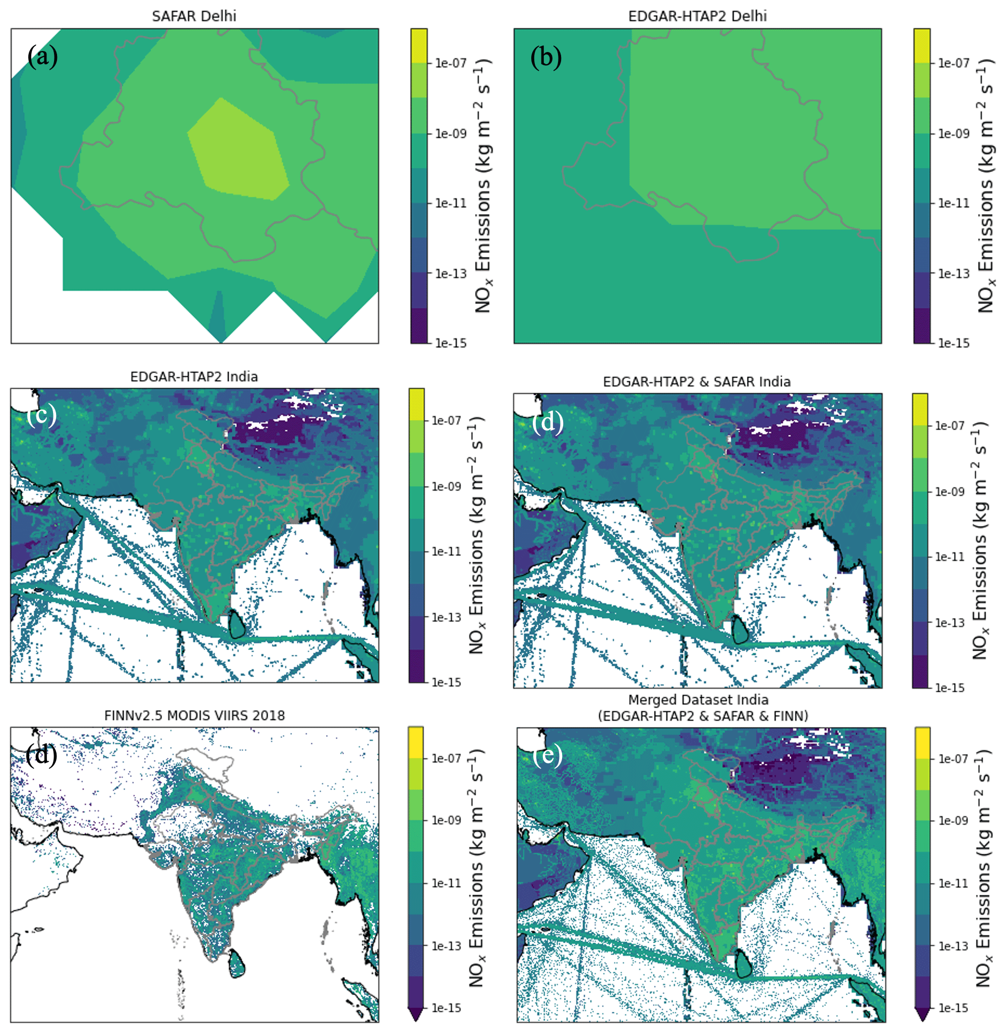
Figure 1(a) NOx emissions () within Delhi from the System of Air Quality and Weather Forecasting and Research (SAFAR) (Beig et al., 2018) for 2018 regridded from 400 m to 10 km resolution. (b) NOx emissions within Delhi from the Emission Database for Global Atmospheric Research with Task Force on Hemispheric Transport of Air Pollution version 2.2 (EDGAR-HTAP2) (Janssens-Maenhout et al., 2015) emissions for 2010 at 10 km resolution. (c) Global NOx emissions from EDGAR-HTAP2 for 2010 at 10 km resolution. (d) Merged EDGAR-HTAP2 and SAFAR NOx emissions, where EDGAR-HTAP2 NOx emissions within Delhi have been replaced with NOx emissions from SAFAR. (e) Global fire emissions provided by the FINNv2.5 dataset for 2018 at 10 km resolution. (e) Merged anthropogenic and fire NOx emissions dataset, where SAFAR, EDGAR-HTAP2 and FINNv2.5 emissions have been combined.
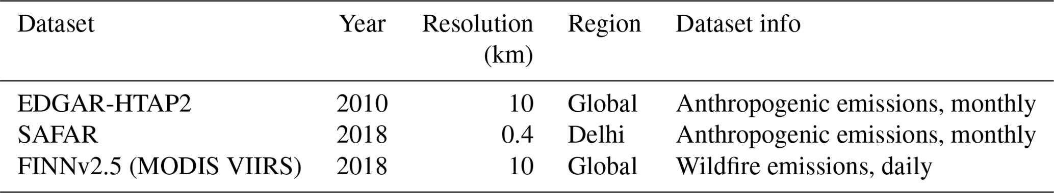
Table 1Details of the anthropogenic and fire emissions datasets used in this study. These were combined to generate daily emissions for India and the surrounding region.
2.1.1 Global emissions
Global monthly NOx emissions are from the Emission Database for Global Atmospheric Research with Task Force on Hemispheric Transport of Air Pollution (EDGAR-HTAP2) 2010 dataset (Janssens-Maenhout et al., 2015), which are at 10 km resolution (Fig. 1c). A comparison between emissions over Delhi from the SAFAR and EDGAR-HTAP2 emissions datasets is also shown in Fig. 1a and b. This clearly demonstrates the SAFAR dataset provides more spatial detail than EDGAR-HTAP2. EDGAR-HTAP2 is a global, gridded air pollution emission inventory compiled using officially reported, national gridded inventories; if national emissions datasets for specific sectors were not available EDGAR v4.3 grid maps were used. The resulting EDGAR-HTAP2 dataset provides a monthly and annual emission distribution along with emission factors that are fuel-, technology-, process- and human-activity-dependent. Emissions include all anthropogenic emissions except large-scale biomass burning (e.g. wildfires).
2.1.2 Delhi emissions
Monthly anthropogenic NOx emissions for Delhi are taken from the 2018 System of Air Quality and Weather Forecasting and Research (SAFAR) dataset (Beig et al., 2018) (Fig. 1a). Data for the SAFAR emission inventory were collected during a 37 500 h campaign and are provided at very high (400 m) resolution over a region covering 70 km×65 km. Emissions are provided for 26 different source sectors. Emissions are very detailed; for example, emissions for transport were calculated using traffic volume collected by click counters across the region. Collected data were then converted into emissions using a Geographical Information System (GIS)-based statistical model. Since SAFAR provides a much more detailed and up-to-date inventory of emissions in Delhi, we regrid SAFAR emissions to 10 km and then replace all EDGAR-HTAP2 emissions (see Sect. 2.1.1 for more details) in Delhi with SAFAR emissions using a simple mask method. We create an empty 10 km global grid and first add SAFAR emissions. Then we add EDGAR-HTAP2 emissions where the grid is still empty (i.e. where no SAFAR emissions were added). The combined dataset is resampled to daily resolution by interpolating monthly values to daily temporal resolution.
2.1.3 Fire emissions
Wildfire NOx emissions for 2018 are taken from the Fire Inventory from NCAR (FINNv2.5) dataset (Wiedinmyer et al., 2023) at 10 km resolution (Fig. 1e) and added to the anthropogenic emissions dataset (to generate Fig. 1f). FINNv2.5 combines data from the Moderate Resolution Imaging Spectroradiometer (MODIS) sensors on NASA's Terra and Aqua satellites with the Visible Infrared Imaging Radiometer Suite (VIIRS) on Suomi NPP. We chose to use FINNv2.5 because of its improved ability to detect small, low-temperature fires, which are likely to be important in India (e.g. agricultural burning). Both MODIS and VIIRS use a thermal anomalies product to provide detections of active fires. MODIS detections are provided at 1 km resolution, while VIIRS has a resolution of 375 m. In FINN, fire hotspot detections from MODIS and VIIRS are combined with land cover, biomass consumption estimates and emission factors to calculate daily fire emissions globally at 1 km resolution. The burned area is assumed to be 1 or 0.14 km2 for each fire identified by MODIS or VIIRS, respectively, and scaled back based on the density of vegetation from the MODIS Vegetation Continuous Fields (VCF) (i.e. if 50 % bare = 0.5 or 0.07 km2 burned area). The type of vegetation burned during a detected fire is determined using the MODIS Collection 5 Land Cover Type (LCT). Each fire pixel is assigned to 1 of 16 possible land cover/land use types. The 16 land cover types are then aggregated into eight generic categories to which fuel loadings are applied (Wiedinmyer et al., 2011). Fuel loadings are from Hoelzemann et al. (2004), and emission factors are from Andreae and Merlet (2001), McMeeking (2008) and Akagi et al. (2011). FINN includes all emissions from above-ground vegetation but not from the combustion of peat (Kiely et al., 2019). Fire types included are wildfires and prescribed and agricultural burning. However, trash burning or biofuel use are not included.
The merged emission dataset described above provides the control scenario in which all sectors are included (Fig. 1f). Additionally, a further six emissions files were generated where individual sectors are excluded (transport, industry, power, residential, other and fires) to quantify their contribution to accumulated NOx along the trajectory path.
2.2 Satellite data
We use tropospheric column nitrogen dioxide (TCNO2) measurements for February 2018 to January 2020 from the TROPOMI instrument aboard ESA's Sentinel-5 Precursor (S5P) satellite that was launched on 13 October 2017. TROPOMI is a hyper-spectral nadir-viewing imager with an Equator overpass time at an ascending node of 13:30 LT. The NO2 columns are derived using TROPOMI's UVIS spectrometer backscattered solar radiation measurements in the 405–465 nm wavelength range (van Geffen et al., 2015, 2022). The swath is divided into 450 individual measurement pixels, which results in a near-nadir resolution of 7.0 km×3.5 km. The total NO2 slant column density is retrieved from the level-1b UVIS radiance and solar irradiance spectra using differential optical absorption spectroscopy (van Geffen et al., 2022). Tropospheric and stratospheric slant column densities are separated from the total slant column using a data assimilation system based on the TM5-MP chemical transport model, after which they are converted into vertical column densities using a lookup table of altitude-dependent air mass factors. As data were available from February 2018 onwards, we selected the 2 years (2018–2019) closest to the back trajectories (2017–2018) and anthropogenic (2010/18) and fire emissions (2018) for our analysis. We follow the approach of Pope et al. (2018) to map TROPOMI TCNO2 data onto a grid over India. The approach of Pope et al. (2018) uses an oversampling methodology where TROPOMI pixels are sliced into sub-pixels and mapped onto a high-resolution level-3 grid. Individual retrievals are filtered for a geometric cloud fraction <0.2 and a quality control flag >75 using all the available daily TROPOMI data for both years.
2.3 Back trajectories
Our approach is to combine back trajectories with top-down satellite TCNO2 or bottom-up NOx emission estimates to investigate the influence of long-range transport (advection) of NOx on Delhi AQ under different wind directions. In the following section we refer to bottom-up NOx emissions; however, the method is the same when using satellite TCNO2.
We use primary NOx emissions integrated over air mass back trajectories to determine the relative influence of direct NOx emissions on those air masses. Back trajectories are calculated using the Reading Offline Trajectory (ROTRAJ) Lagrangian transport model (Methven et al., 2003). The model uses dynamical fields from ERA-Interim reanalysis from the European Centre for Medium-Range Weather Forecasts (ECMWF) to calculate trajectories at 1.125∘ horizontal resolution. After a trajectory parcel is released, its location is calculated every 6 h; for vertical interpolation the model uses cubic Lagrangian interpolation, and horizontal fields are calculated using bilinear interpolation. This approach primarily focuses on large-scale advection and does not resolve small-scale sub-grid turbulent transport or convection.
In this study, ROTRAJ back trajectories were released from just above the surface (0.99 sigma level; a terrain-following coordinate system where 1 is the surface) in central Delhi at 06:00 UTC (11:30 LT) for the years 2017 and 2018, extending back 4 d in 6 h time steps. We choose 06:00 UTC (11:30 LT) as this is close to midday local time and so matches the time of the satellite overpass time (13:30 LT) most closely. We are restricted to using ROTRAJ back trajectories for 2017 and 2018, while using satellite data for 2018 and 2019, as the ECMWF ERA-Interim reanalysis dataset was terminated in August 2019 and satellite data are not available until 2018. NOx emissions were accumulated along each trajectory over 4 d at 15 min time intervals (interpolated linearly from 6-hourly position output) (Fig. 2).
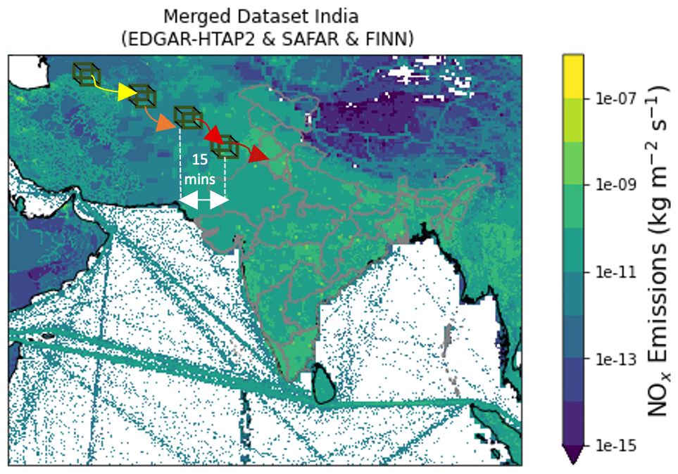
Figure 2Back-trajectory method used in this study. Gridded emissions from a bottom-up inventory (Fig. 1e) are summed every 15 min (15 min) along the back-trajectory path (arrows) when the air parcel is within the boundary layer (indicated by boxes). NOx accumulates along the trajectory path towards Delhi (indicated by line shading). Satellite tropospheric column NO2 (TCNO2) is also summed in a similar way.
NOx emissions were only accumulated if the trajectory path was within the boundary layer (which we determine based on ERA-Interim reanalysis). At each location, we accumulate the entire emission within an emission grid box (TCNO2: ∼5 km; emissions: ∼10 km) over which the trajectory passes. The surface area of each grid box that the trajectory points passed over is also accumulated over time.
The along-trajectory emission accumulation can be represented by Eq. (1):
where N (=384) and E0=0.0.
Ei is the accumulated NOx (kg) at any given point i along the trajectory (with E at point 0 [E0] being equal to 0), ϕi is the emissions flux of NOx () at point i, Δt is the 15 min time step, α at point i is the surface area of the grid box (m2) and τ at point i is the specified NOx lifetime (τ). Therefore, E is total accumulated NOx mass (kg) and N is the number of 15 min time steps within the 4 d trajectory (384).
To account for chemical loss of NOx along the trajectory path, the lifetime of NO2 was calculated at each time step from TOMCAT (Chipperfield, 2006; Monks et al., 2017) 3-D hourly hydroxyl radical (OH), pressure and temperature fields, assuming the main loss pathway in Eq. (2), where NO2 is oxidised by OH to form nitric acid (HNO3) (which dominates over photolysis within the boundary layer). The NOx lifetime (τ) (Eq. 3) was calculated using a temperature and pressure-dependent rate constant (k) (IUPAC, 2021). The calculated lifetime (τ) was then applied to the total NOx accumulated emission in the air parcel in Eq. (1).
To remove the dependence of the accumulated emissions calculated in Eq. (1) on emission grid resolution (since we assumed the air mass has the same width as the emission grid box), the total accumulated NOx mass (E) was divided by accumulated surface area (S) and then scaled by 109 to give E units of µg m−2. S is given by Eq. (4):
Emissions accumulated within Delhi (EDelhi) were also determined using the same approach but only implemented when the trajectories enter the Delhi region, which we define using a bounding box (28.1–28.9∘ N, 76.8–77.5∘ E). To derive EDelhi in units of µg m−2, the accumulated NOx mass from Delhi was divided by the accumulated surface area (S) over the full trajectory path. The ratio between represents the fractional contribution of Delhi sources towards the total accumulated NOx emissions.
Finally, the daily (06:00 UTC) total accumulated emission and ratios from all sites were binned by eight wind directions (north through to north-westerly) based on their end point in relation to Delhi. This methodology provides a powerful tool to identify which flow directions are the most polluted and to derive the proportion of pollutant emissions from long-range transport versus local sources.
2.4 Observational data
Hourly averaged surface NO2 concentrations from 36 sites across the Delhi region for 2018 and 2019 (Fig. 3) were obtained from the CAAQMS (Continuous Ambient Air Quality Monitoring Stations) portal (https://app.cpcbccr.com/ccr/#/caaqm-dashboard-all/caaqm-landing, last access: 7 October 2022) of the Central Pollution Control Board (CPCB) of India. The ambient NO2 concentration was measured based on the gas phase chemiluminescence methodology; the technical details of monitoring can be found in CPCB (2019). The data were further quality controlled to remove outliers and missing values (Singh et al., 2020). As TROPOMI has a local overpass time of approximately 13:30, the average NO2 between 13:00–14:00 LT was calculated for each site to represent the daily NO2 corresponding to the overpass of TROPOMI. From this, the daily median NO2 concentration across all sites was calculated to represent daily NO2 levels over Delhi in 2018 and 2019.
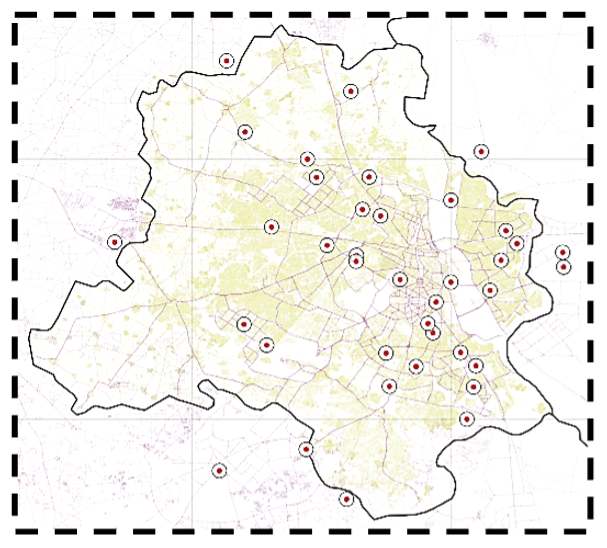
Figure 3Map showing the location of NO2 monitoring sites across the Delhi region (n_sites = 36). In this study we use the daily 07:30–08:30 UTC (13:00–14:00 LT) median NO2 concentration (calculated using all sites shown) to determine the timing of high-pollution days in Delhi. We define high-pollution days as days where the NO2 concentration exceeds the 90th percentile of NO2 concentrations between 2018 and 2019.
3.1 TCNO2 back-trajectory analysis
The contribution of local and non-local sources to NO2 levels in Delhi is controlled by primary emissions, the chemical lifetime of NO2 and advection by meteorology (i.e. accumulation/advection of pollutants under stable conditions or ventilation of source emissions downwind). Figure 4b–d show the annual average TCNO2, surface NO2 lifetime and boundary layer height (BLH) over India along with the anomalies for the pre-monsoon (February–May), monsoon (May–October) and post-monsoon (October–February) seasons.
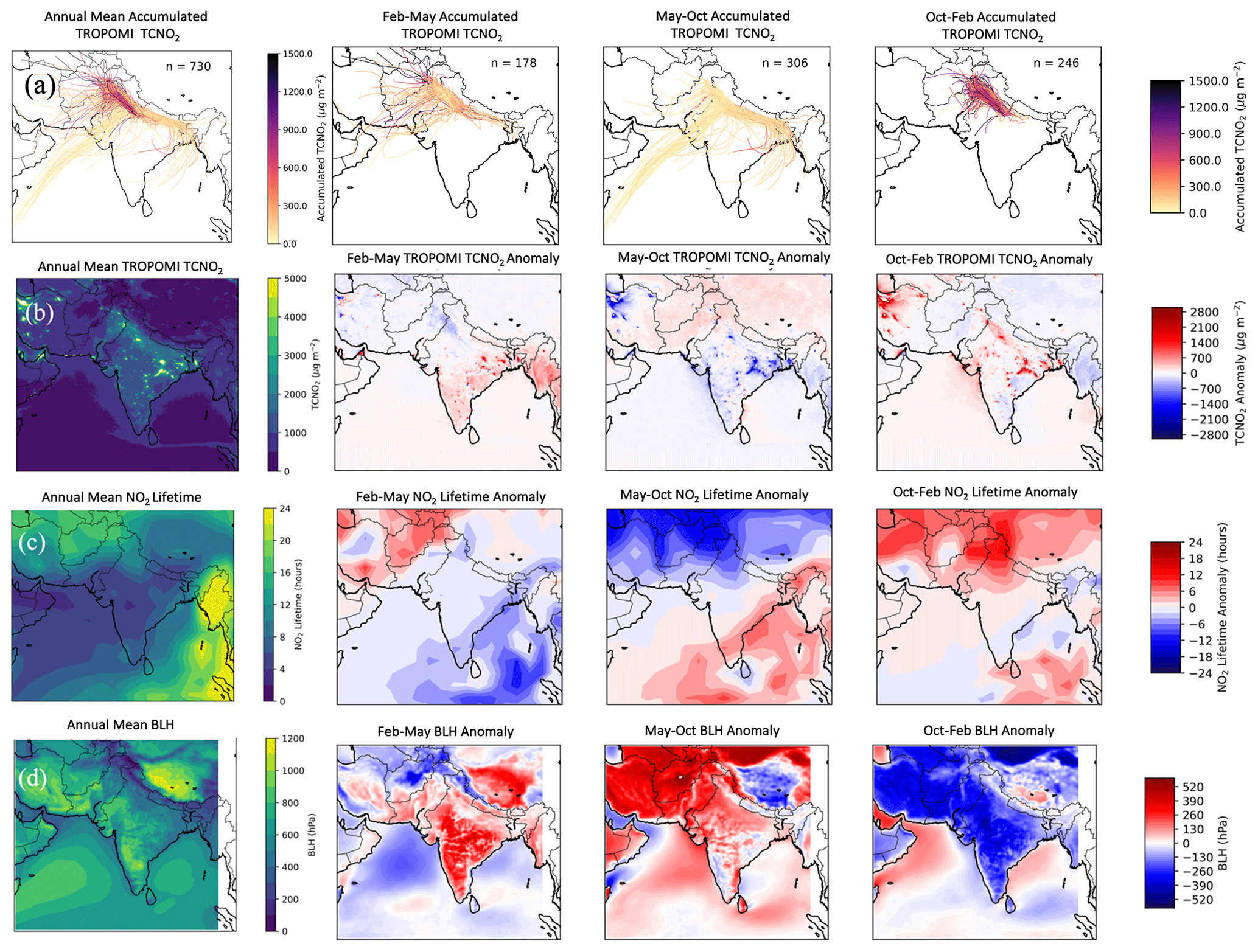
Figure 4(a) Total annual (and seasonal) accumulated TROPOMI TCNO2 (µg m−2) arriving in Delhi along 4 d back trajectories. Trajectories are coloured by their total accumulated TCNO2, with darker trajectories indicating higher levels of accumulated TCNO2. (b) Mean annual (and seasonal) TCNO2 (anomaly) (µg m−2), (c) mean annual (and seasonal) NO2 lifetime (anomaly) (h) and (d) mean annual (and seasonal) boundary layer height (BLH) (anomaly) (hPa) compared to all seasons. All panels show the time period of 2017 and 2018 annually and seasonally – during the pre-monsoon (February–May), monsoon (May–October) and post-monsoon (October–February) seasons, respectively.
Peak annual TCNO2 ranges between 4000 and 5000 µg m−2 over the source regions (e.g. Delhi, Kolkata, Nagpur and industrial sources in the east (approximately 20–25∘ N, 80–85∘ E)) (Fig. 4b). Smaller urban NO2 hotspots range between 3000 and 4000 µg m−2, higher than values across large European hotspots, which peak at 3500 µg m−2 (Pope et al., 2019). In the seasonal anomaly, the pre-monsoon TCNO2 values increase by approximately 500–1000 µg m−2 around Delhi but with similar decreases to the north-west. However, the majority of the country experiences TCNO2 increases greater than 2000 µg m−2. During the monsoon season there is a decrease in TCNO2 by 1000–1500 µg m−2 over Delhi, which is reflected in most other urban centres and industrial regions. The post-monsoon season experiences the largest degradation in NO2-related air quality as all hotspots increase by >2000 µg m−2 (e.g. for Delhi), with peak enhancements over the industrialised region in the east of India and to the north-west of Delhi in Punjab and Haryana, where agricultural burning is common during this time.
The calculated NO2 lifetime (based on modelled OH, temperature and pressure) typically ranges between 1.5 and 15 h over India (between 20 and 24 h over Bangladesh and Myanmar) and between 8 and 12 h over Delhi (Fig. 4c). During the pre-monsoon season, there is little change from the annual average, decreasing by 1 to 2 h over Delhi. Along the east Indian coastline, there is a general decrease of 3–5 h. During the monsoon season, there are large reductions in the NO2 lifetime over the northern segment of the domain, decreasing by 5 to 10 h and propagating southwards to Delhi with a decrease of approximately 3–5 h. Central India remains similar to the annual average, while the east coastline now experiences increases in the NO2 lifetime of 3 to 5 h. In the post-monsoon season, while southern India experiences little change, Delhi and the north of India see an increase in the lifetime by 3–7 h.
Western India has an annual average BLH ranging between 800 and 1100 m (400–800 m over eastern India), while the Delhi BLH is between 400 and 600 m (Fig. 4d). In the pre-monsoon season, the Indian boundary layer is well ventilated with an increase in BLH by ∼200 to 400 m (50–100 m for Delhi). In the monsoon season, the boundary layer remains well ventilated with enhancements of typically 100 to 200 m (although with some regions of reduction in the BLH), relative to the annual average. In the post-monsoon season, colder temperatures cause countrywide shallowing of the boundary layer by 200 to 400 m, including Delhi, peaking at over 500 m in central India.
During the pre-monsoon and, especially, post-monsoon seasons, conditions are favourable for the degradation of NO2 air quality. In the pre- and post-monsoon seasons, primary NOx emissions (e.g. from increased domestic heating, power demands and agriculture burning) are typically larger, and there is a longer NO2 lifetime (i.e. less chemical loss) and a shallower boundary layer, trapping emissions over Delhi and the wider IGP. This effect is largest in the post-monsoon season, though it is also apparent in the pre-monsoon season. In contrast, during the monsoon there are lower primary NOx emissions, a shorter NO2 lifetime and increased atmospheric ventilation of the boundary layer, all of which yield lower pollution levels during the monsoon season. We have thus demonstrated the seasonal influences on NO2 levels in Delhi and the surrounding region but now exploit the back-trajectory integrated emissions methodology (see Sect. 2) to determine the balance of local versus non-local sources of NOx in Delhi air quality. Here, we accumulate TCNO2 from TROPOMI under the back trajectories to investigate the seasonal influence of wind direction on the advection of TCNO2 into Delhi. As discussed above, there is a clear seasonal influence of the monsoon circulation on the back-trajectory integrated emission totals.
On average, the back trajectories arrive in Delhi at the surface from the south-west, east and north-west (Fig. 4a). Trajectories from the south-west have the lowest accumulated TCNO2 levels (0–200 µg m−2), largely originating over the Arabian Sea (i.e. fewer NOx sources) before arriving in Delhi. Trajectories originating from east India pass over several large urban centres and industrial regions, yielding integrated TCNO2 trajectories with TCNO2 levels that range between 400 and 900 µg m−2 before arriving in Delhi. The trajectories from the north-west are the most polluted, with peak TCNO2 levels of >1500 µg m−2. When split seasonally, the pre-monsoon season shows trajectories approaching Delhi from the north-west (200–>1000 µg m−2) and east (200–900 µg m−2). In the monsoon, cleaner air masses (0–200 µg m−2) originate from the south-west, while many eastern air masses remain polluted similarly to the pre-monsoon season (200–900 µg m−2). During the post-monsoon season, most trajectories are from the north-west of India and show the largest seasonal pollution levels (i.e. integrated TCNO2 back trajectories of typically 600 to >1500 µg m−2), suggesting that agricultural waste burning in north-west India contributes to poor AQ in Delhi during this time.
3.2 NOx emissions back-trajectory analysis
We repeated this approach using the bottom-up emissions inventory (Fig. 5), finding that the results are generally in close agreement to the TCNO2 results, with the highest accumulated emissions being observed in the pre- and post-monsoon seasons. In the pre-monsoon season, the integrated emission back trajectories range between 100 and 800 µg m−2 from both the east and north-west. Note that the emission trajectory values are lower than the equivalent TCNO2 values as they are emission fluxes and not the tropospheric integrated column. In terms of altitude, the trajectories range from the near-surface to 400 hPa. At t=96 h before arrival at Delhi, the median trajectory position is near 800 hPa before descending below 950 hPa at approximately 30 h from Delhi (t=30 h). In the vertical distribution, there is no clear link between the integrated emission trajectory values and altitude. During the monsoon season, there are two limbs of integrated emission trajectories, with TCNO2 ranging between 0 and 400 µg m−2 from the south-west and between 300 and 500 µg m−2 from the east. The average trajectory position is lower in altitude, starting at approximately 950 hPa and remaining below this pressure level. There appears to be a split in the trajectory origins and altitudes with south-western trajectories coming from the Arabian Sea near the surface with few emissions sources (air masses will be influenced to some extent by shipping emissions, but the short NO2 lifetime will yield limited impact in Delhi), while more polluted trajectories (i.e. substantial upwind sources) from the east are typically 900–600 hPa in altitude. During the post-monsoon season, the median trajectory altitude is approximately 875 hPa at t=96 h before arrival in Delhi. For the final 24 h or so, the trajectories converge on Delhi below 950 hPa. As a result, while all seasons experience trajectories 1 d out from Delhi below 950 hPa, the post-monsoon trajectories are closer to the surface than the pre-monsoon equivalent throughout the 4 d and are exposed to larger emission fluxes than those during the monsoon. Secondly, as these post-monsoon trajectories originate from the north-west and are trapped in the IGP by the Himalayas, there is the opportunity for re-circulation of the trajectory over upwind NOx sources. Overall, the meteorological, chemical and emission factors, all trapped against the Himalayas, in the post-monsoon season are key for the substantial degradation in the air quality.
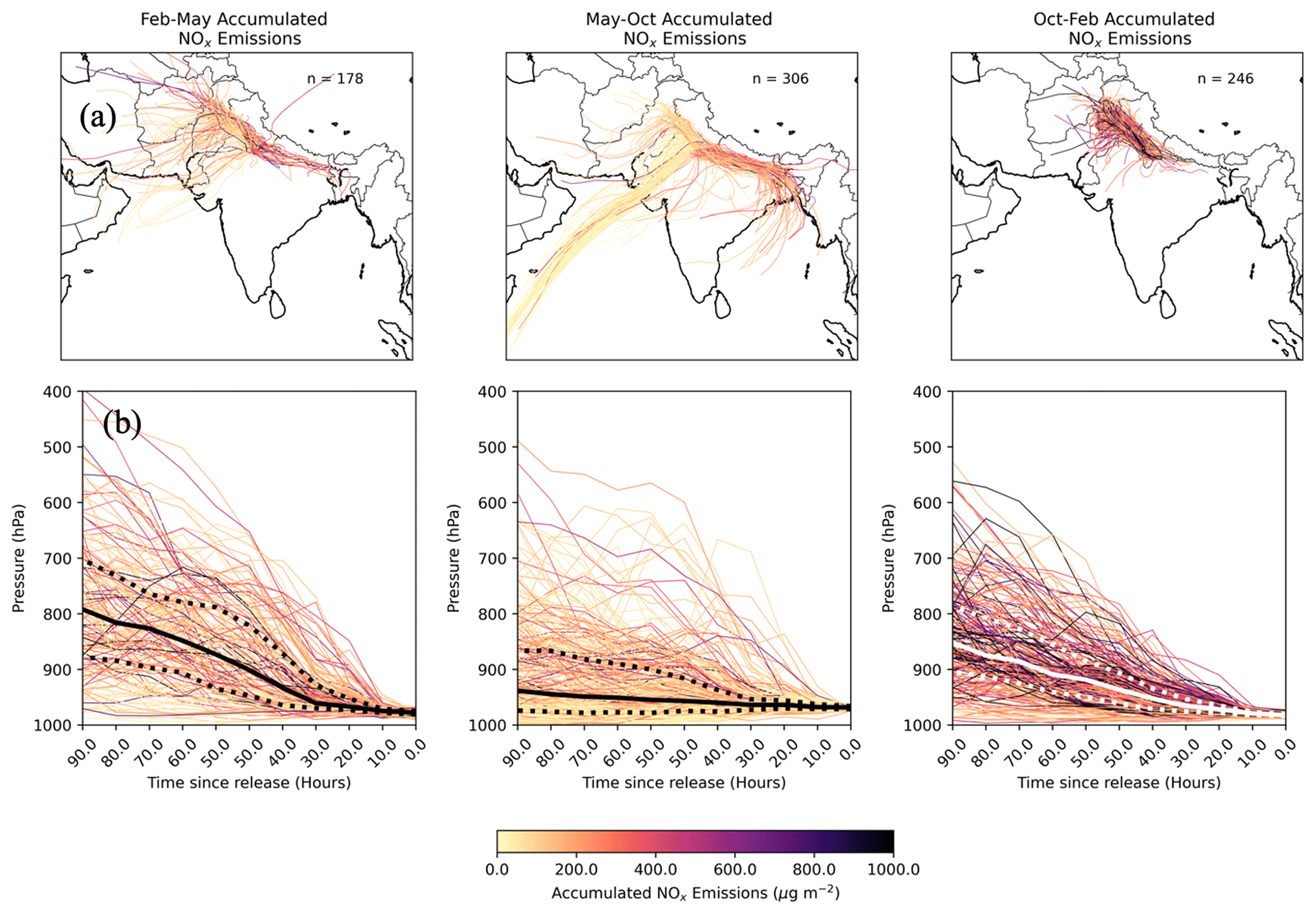
Figure 5(a) Total accumulated NOx emissions (µg m−2) arriving in Delhi in 2017 and 2018 and (b) pressure level of air parcels as they converge on Delhi, just above the surface (∼1000 hPa) at hour 0 in pre-monsoon (February–May), monsoon (May–October) and post-monsoon (October–February) seasons. Median (black/white line) and 25th and 75th percentiles (black/white dashed lines) of the trajectory pressure are also indicated. Trajectories are coloured by their total accumulated emissions, with darker trajectories indicating higher levels of accumulated NOx.
The integrated emission trajectories also provide the opportunity to gain better insight about the proportion of local vs. non-local sources (i.e. integrated trajectories over the full 4 d vs. integrated trajectories just over Delhi). Figure 6 shows this, but note that we only plot wind directions where the sample size is greater than or equal to 10. We find that during the pre-monsoon season, the grouped integrated emissions trajectories are moderately polluted (south-west, west and north-west) and range between 30 and 120 µg m−2, with peak average north-westerly and easterly values of approximately 300 µg m−2. In terms of local contributions, all flows are dominated by local sources (i.e. 75 %–100 %). During the monsoon, all wind directions (easterly, south-easterly, south-westerly, westerly and north-westerly) have lower integrated emission back trajectories (integrated NOx emissions peaking at approximately 200 µg m−2), with 80 %–95 % of emissions coming from local sources. For poor air quality, as discussed above, the post-monsoon season is the most important, as integrated emission trajectory values from the north (sample size (n)=17), north-west (n=179), north-east (n=10) and east (n=21) range between 300 and >400 µg m−2 on average. Despite the larger integrated emissions trajectory median values, the key factor is the local contribution is much lower, ranging from 65 %–80 %. The north-westerly trajectory median accumulated NOx emissions are the largest and most frequent (i.e. 73 % of trajectories originate from the north-west) during the post-monsoon season, with approximately 35 % of emission contributions coming from outside of Delhi. Thus, we find that the advection of highly polluted air originating from both inside and outside Delhi is an important contributor to the Delhi population, and air quality mitigation strategies need to be adopted not only in Delhi but also in the surrounding regions to successfully control this issue.
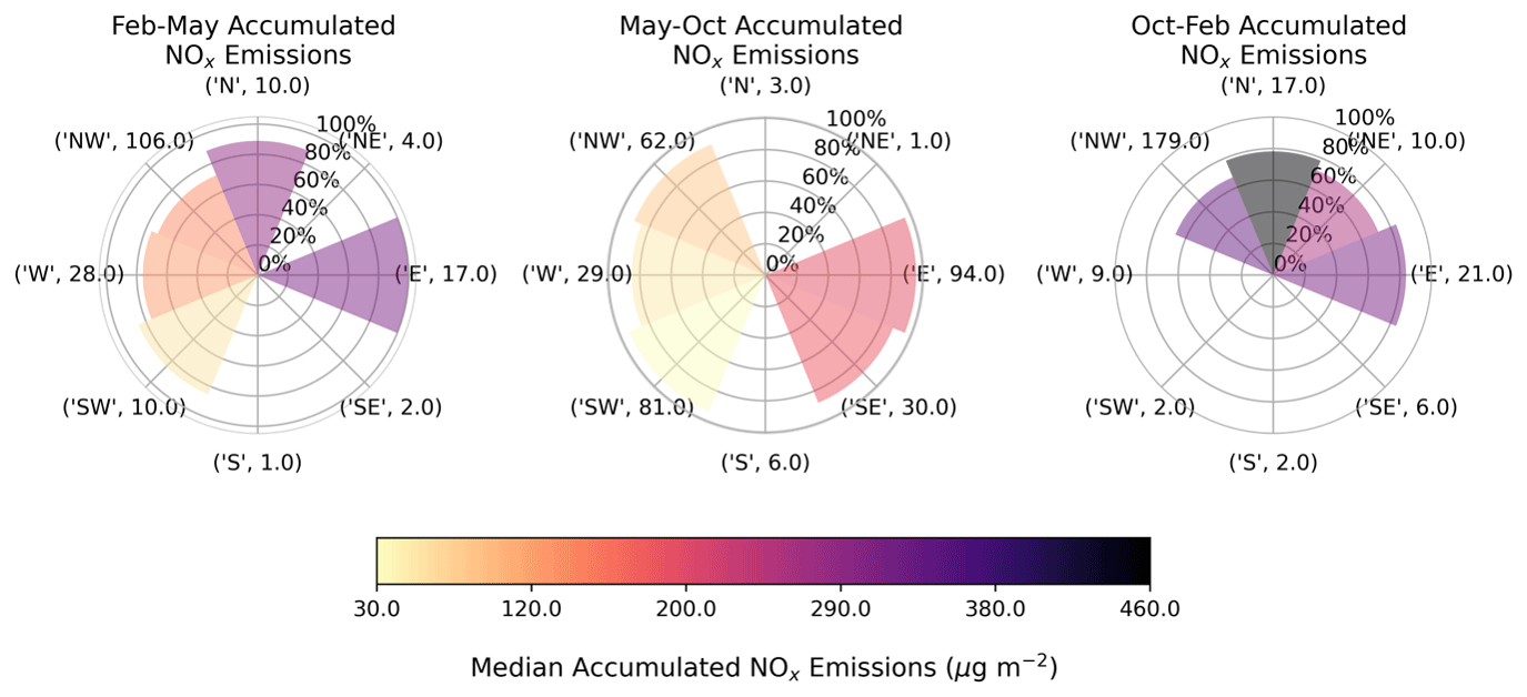
Figure 6Wind rose of median accumulated NOx emissions (µg m−2) from 4 d back trajectories with 6 h time steps arriving at Delhi in 2017 and 2018 for pre-monsoon (February–May), monsoon (May–October) and post-monsoon (October–February) seasons. Total accumulated emissions are indicated by the shading of the segments. The area of the segment indicates the non-local contribution to the total integrated emissions. The percentage of local emissions is indicated on the circles. The number of days on which each wind direction occurs in each season is also indicated in brackets. For example, NW in the post-monsoon season is very polluted (∼350 µg m−2), 65 % of total integrated emissions are non-local and this wind direction occurs on 179 d.
3.2.1 Contribution of individual emissions sectors
Next, we quantify the influence of individual sectoral emissions on the total accumulated emissions by running the back-trajectory analysis without individual emissions source sectors and analysing accumulated emissions (Fig. 7; note that only wind directions with a sample size greater than or equal to 10 are shown). During the pre-monsoon season, accumulated emissions from the transport sector are the dominant contributor (>70 %), and, though local sources dominate (>70 %), non-local sources are also important (30 %) under the most frequent north-westerly and westerly wind directions. Trajectories travel close to the surface, within the boundary layer, in the final 24 h, and the NOx lifetime is short. This indicates that a large fraction of the total integrated emissions reaching Delhi are likely to have originated in the region surrounding the city, where the NOx burden from transport is high. Additionally, the contribution of local industrial and other emissions is evident.
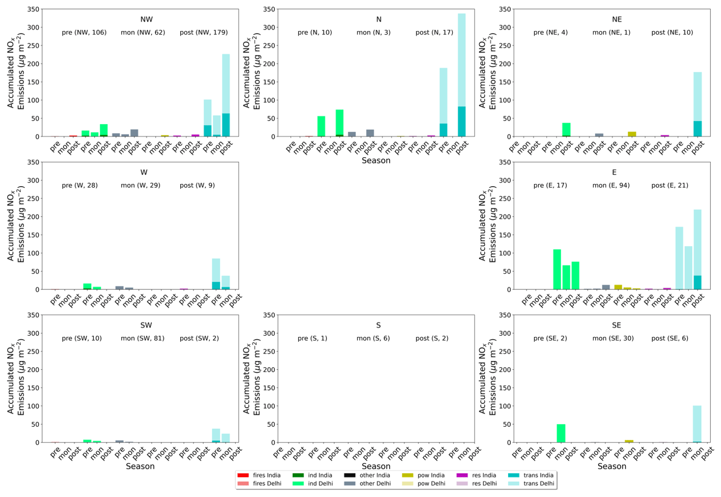
Figure 7Sector-specific accumulated NOx emissions (µg m−2) from 4 d back trajectories with 6 h time steps arriving in Delhi in 2017 and 2018 in the pre-monsoon (pre) (February–May), monsoon (mon) (May–October) and post-monsoon (post) (October–February) seasons. Light shading indicates accumulated NOx emissions originating within Delhi, and darker shading indicates accumulated NOx emissions originating from outside of Delhi. Sectors included are fire (FIRES) (red), industrial (IND) (green), other (OTHER) (black), power generation (POW) (gold), residential (RES) (magenta) and transportation (TRANS) (cyan) emissions. The number of days for which each wind direction occurs in each season is indicated in brackets. For example, north-westerly winds occur on 179 d during the post-monsoon season and transport emissions dominate (∼80 µg m−2). The contribution from transport is split into ∼55 µg m−2 for non-local (India) and ∼25 µg m−2 for local (Delhi).
During the monsoon season, easterly (easterly and south-easterly) and westerly (south-westerly and north-westerly) winds dominate. Under all directions, local accumulated emissions show nearly similar contribution (>90 %) for all sectors. Although many trajectories travel from distant regions, remaining close to the surface, there are few sources over the ocean (apart from shipping) and the NOx lifetime is short, so the advection of accumulated emissions concentration is much lower. Therefore, the small contribution of non-local sources is likely from nearby regions within the polluted IGP. Overall, transport emissions have the highest contribution to overall accumulated emissions (>70 %), which is likely driven by transport emissions dominating the NOx burden in Delhi. In addition, contributions from local power and industrial emissions are also important under easterly and south-easterly (and north-westerly) wind directions, with only a small non-local contribution to the overall emissions (<10 %), and are likely to originate from the large industrial region to the east of Delhi and from power generation to the north-west.
During the post-monsoon season, winds are primarily north-westerly and are associated with high contributions from transport emissions (>70 % transport, 70 % local emissions), with non-negligible contributions from industry, other, power and residential emissions (and negligible contributions from fires). Again, local sources generally dominate for these sectors, except residential and power (85 % and 100 % non-local), which have the largest probable contribution from within the IGP region surrounding Delhi, where residential emissions are high, and to the north-west, where many power stations are located. This suggests the increase in accumulated NOx emissions during the post-monsoon season is driven by a combination of several factors. First, a longer NOx lifetime, arising from OH being less abundant (to react with NOx), enables accumulated emissions to be advected over long (and short) distances from high-emission regions north-west of Delhi, increasing the contribution of non-local sources to AQ in Delhi. Second, a shallow boundary layer traps emissions close to the surface, allowing local emissions to accumulate, as well as allowing the accumulation of emissions along the trajectory path. Third, there is an increase in emissions during winter months due to increased demand for heating (residential sector) and power (power sector).
3.2.2 High-pollution events
Finally, we apply the same back-trajectory emissions method to the high-pollution days in Delhi to investigate the drivers of high-pollution events in the city. We use daily median ground-based NO2 observations from sites in Delhi and the surrounding region to identify high-pollution days, defined as days where daily median NO2 concentrations are above the 90th percentile of daily median NO2 concentrations (>37 µg m−3) between 1 January 2017 and 31 December 2018 (Fig. 8a). We then subsample the trajectories using these high-pollution days and attribute the accumulated emissions to specific emissions sectors.
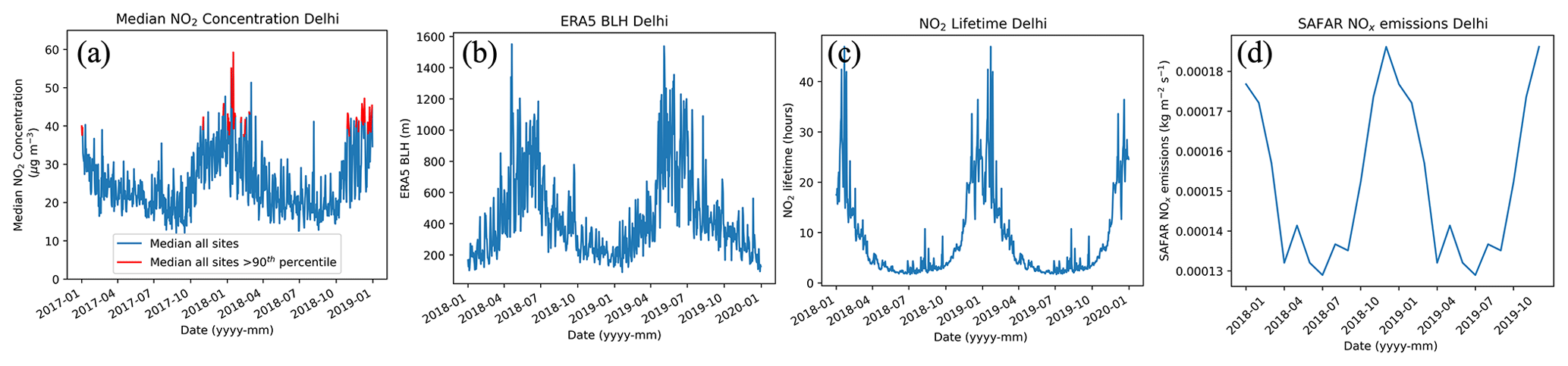
Figure 8(a) Daily median NO2 concentrations (µg m−3) in Delhi (blue). Concentrations above the 90th percentile of observations are indicated in red. (b) Daily mean boundary layer height (BLH) (m) in Delhi from ERA5 re-analysis, (c) daily mean NOx lifetime (h) in Delhi and (d) monthly mean NOx emissions () from the SAFAR emissions inventory. All panels show the time period between 1 January 2017 and 31 December 2018.
There is a clear seasonal cycle in NO2 concentrations in Delhi, with maximum NO2 values occurring during pre- and post-monsoon seasons that peak in December (up to ∼60 µg m−3) and minima during monsoon seasons (20 to ∼30 µg m−3) (Fig. 8a). We also find that BLH is inversely related with median NO2 concentrations, indicating a shallow boundary layer (<600 m) during the pre- and post-monsoon seasons and a higher boundary layer (600–1500 m) during the monsoon (Fig. 8b). Additionally, the atmospheric lifetime of NOx is highest in pre- and post-monsoon seasons (>10–70 h) and is lowest during the monsoon season (∼10 h) (Fig. 8c). Finally, NOx emissions are also highest during the pre- and post-monsoon seasons (∼0.05–0.07 ) and lowest during the monsoon season (<0.055 Fig. 8d). The combination of these factors aids the accumulation of increased local emissions during the pre- and post-monsoon seasons and the dispersal of the decreased emissions during the monsoon. Thus, the non-monsoon seasons, especially in the post-monsoon season, experience a substantial degradation in air quality.
The back-trajectory emissions analysis indicates that high-NO2-pollution days are associated with trajectories from the north-west of Delhi (Fig. 9a) in both the pre-monsoon (n=12 d) and post-monsoon (n=60 d) seasons. Note that we only include wind directions with a sample size greater than or equal to 5 (easterly and north-westerly). Trajectories gradually descend towards the surface between 90 and 20 h out from Delhi, remaining close to the surface (>950 hPa) until they reach Delhi (Fig. 9b). However, during the post-monsoon season, trajectories are much closer to the surface from hour 90 (910–810 hPa) compared with the pre-monsoon season (840–770 hPa), likely allowing increased accumulation of emissions. During post-monsoon high-pollution days, local (∼70 % local) transport emissions dominate (>75 %) the total accumulated emissions (Fig. 10). This is likely due to the trajectories remaining close to the surface for the final 24 h, within a shallow boundary layer, at a period when the NOx atmospheric lifetime and emissions are increased. The contribution of other sectors to the remaining accumulated emissions (residential, industrial, other and power) is smaller, but local emissions remain important (25 %–100 %). There is also a negligible contribution (<2 µg m−3) from non-local (100 %) fires under north-westerly winds. Overall, this suggests that non-local NOx emissions from long-range transport (advection) contribute to poor NO2 AQ in Delhi, but the accumulation of local emissions under a shallow boundary layer dominates.
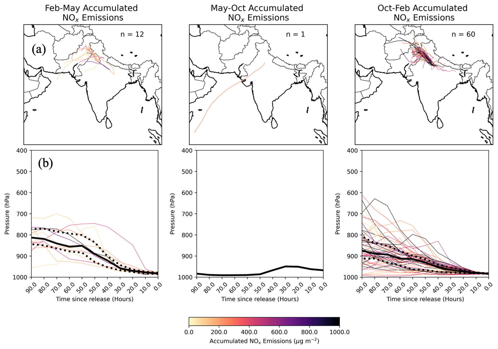
Figure 9(a) Total accumulated NOx emissions (µg m−2) arriving at Delhi during high-pollution events in 2017 and 2018, (b) pressure level of air parcels as they converge on Delhi just above the surface (∼1000 hPa) at hour 0 in pre-monsoon (February–May), monsoon (May–October) and post-monsoon (October–February) seasons. Median (black line) and 25th and 75th percentiles (black dashed lines) of the trajectory pressure are also indicated. Trajectories are coloured by their total accumulated emissions, with darker trajectories indicating higher levels of accumulated NOx.
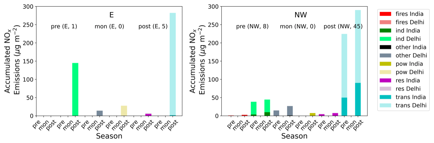
Figure 10Sector-specific accumulated NOx emissions (µg m−2) from 4 d back trajectories with 6 h time steps arriving at Delhi during high-pollution events in 2017 and 2018 in the pre-monsoon (pre) (February–May), monsoon (mon) (May–October) and post-monsoon (post) (October–February) seasons. Light shading indicates accumulated NOx emissions originating within Delhi and darker shading accumulated NOx emissions from outside of Delhi. Sectors included are fire (FIRES) (red), industrial (IND) (green), other (OTHER) (black), power generation (POW) (gold), residential (RES) (magenta) and transportation (TRANS) (cyan) emissions. The number of days for which each wind direction occurs in each season is indicated in brackets. For example, north-westerly winds occur on 45 d during high-pollution days in the post-monsoon season, and transport emissions dominate (>250 µg m−2). The contribution from transport is split into ∼80 µg m−2 for non-local (trans India) and ∼200 µg m−2 for local (trans Delhi).
4.1 Seasonal wind flow regimes
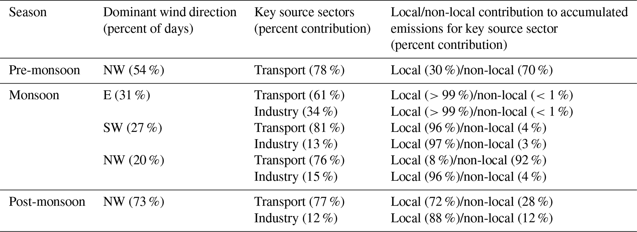
In this study we have used high-resolution satellite tropospheric column NO2 (TCNO2) data from TROPOMI and bottom-up NOx emission inventories alongside a back-trajectory model to investigate the relative contribution of local and non-local pollutants to air quality in Delhi throughout the year. We also performed sensitivity simulations to separate the influence of various sectoral emissions on the accumulated pollution by removing individual emission source sectors. We summarise our findings in Table 2, which gives the dominant wind direction(s) in each season as a percentage of days in the season, the source sectors with the largest contribution to the accumulated emissions under that wind direction, and finally the contribution of local (Delhi) or non-local (rest of India) accumulated emissions to the total accumulated emissions. Our analysis indicates that both TCNO2 and emissions accumulated over 4 d are highest under easterly, northerly and north-westerly directions during the pre-monsoon (TCNO2: 200–1000 µg m−2; emissions: ∼300–800 µg m−2) and post-monsoon (TCNO2: 600–1500 µg m−2; emissions: ∼200–>1000 µg m−2) seasons. During the pre-monsoon season, north-westerly wind directions dominate (54 %). The seasonal satellite TCNO2 anomaly indicates decreased TCNO2 in the north-west of Delhi but increased TCNO2 locally in Delhi, suggesting that local emissions are the dominant influence on AQ in Delhi during this time. In agreement with this, accumulated NOx emissions indicate that emissions from the transport sector account for >70 % of the total accumulated emissions but indicate ∼70 % contribution from local emissions. The high accumulated emissions observed under these wind directions are likely driven by high local NOx emissions during the pre-monsoon season (since NOx lifetime is relatively short and the boundary layer is relatively deep). During the post-monsoon season, north-westerly wind dominates (73 %). The seasonal satellite TCNO2 anomaly indicates increased TCNO2 over Haryana, Punjab and Delhi, suggesting that agricultural waste burning and local emissions are likely to influence AQ in Delhi during this time. In contrast, accumulated NOx emissions indicate that transport emissions (>70 %), which are predominantly local (70 %), are most important. During the post-monsoon season high emissions are accompanied by a longer NOx atmospheric lifetime and shallow boundary layer. These two mechanisms aid the build-up of emissions along the trajectory path and lead to increased advection of NOx into the city under north-westerly flow. In addition, the accumulation of local emissions increases too. Alongside this, local and non-local (50 %–100 %) residential, other and industrial emissions also contribute to the total accumulated emissions under north-westerly winds during the post-monsoon season. Emissions are likely due to increased demand for heating and energy during the colder post-monsoon season in nearby states, such as Uttar Pradesh, where there is a strong reliance on open stoves and fires for cooking and heating.
Table 2Summary of key wind directions in the pre-monsoon (February–April), monsoon (May–September) and post-monsoon (October–January) seasons (as percent of total days in each season). The key source sectors with the largest contribution to the overall total accumulated emissions are also indicated (as percent contribution) alongside the contribution of local (Delhi) and non-local (rest of India) accumulated emissions to overall accumulated emissions for that sector. For example, in the post-monsoon season NW winds occur in 73 % of days, transport emissions contribute 77 % of the overall integrated emissions, and 72 % of transport emissions are local while 28 % are non-local. Seasonal sector-specific accumulated NOx emissions (µg m−2) are calculated from 4 d back trajectories with 6 h time steps arriving in Delhi in 2017 and 2018 in pre-monsoon, monsoon and post-monsoon seasons.
It should be noted that the mismatch between the spatial pattern of TCNO2 anomalies, which clearly indicate increased TCNO2 over agricultural waste burning regions in the post-monsoon season, and the NOx emissions sectoral analysis may suggest fire emissions are underestimated in the fire emissions dataset. The reasons for this are discussed further in Sect. 4.3.
4.2 Source attribution during high-pollution episodes
We also applied the back-trajectory method to high-pollution days, defined as days where median NO2 concentrations (from ground-based observations) are above the 90th percentile. The ground-based observations indicate that high-pollution episodes are most common in the post-monsoon season (>80 % of occurrences) and are dominated by days where winds were from the north-west (>75 %). On these days (north-westerly winds during the post-monsoon season) local (70 %) transport emissions dominate (>75 %). The large contribution of local transport emissions is likely driven by high NOx emissions in a shallow boundary layer, which acts to trap pollutants at the surface, while the increased non-local contribution of transport emissions (30 %) is likely driven by trajectories (air masses) that travel towards Delhi, remaining close to the surface, accumulating increased emissions that are not quickly lost due to decreased sunlight and therefore less abundant OH during winter months.
4.3 Comparison to previous work
The results of this study are in line with previous work by Jethva et al. (2018) and Sembhi et al. (2020). Jethva et al. (2018) used 3 d HYSPLIT back trajectories which were released from three different altitudes (100, 500 and 1500 m) in Delhi each day between October–November 2013–2016 at 13:30 LT. Trajectories were grouped according to the 24 h averaged PM2.5 concentration at the US embassy in Delhi (0 to <100, 100 to <200, 200 to <300 and >300 µg m−3). In most cases, near-surface trajectories passed over crop burning regions in north-west India (Punjab and Haryana) (52 %, 81 %, 89 % and 84 %, respectively). Thus, indicating air masses passing over crop burning regions are associated with increased PM2.5 concentrations in Delhi. In addition, Jethva et al. (2018) estimated that trajectories took around 14–22 h to be advected from Punjab and Haryana to Delhi, indicating the potential for the advection of NOx emissions to Delhi too. Sembhi et al. (2020) used a model to simulate air quality in Delhi during a poor AQ episode in 2016 with and without the implementation of the SSWA. They found that timing shift in agricultural burning in north-west India caused by the introduction of the SSWA contributed only around 3 % to the poor AQ observed, indicating that this was largely driven by other factors. We also find that trajectories originating from the north-west during post-monsoon seasons have a polluted footprint in our analysis of satellite data and emissions. Both previous studies from Jethva et al. (2018) and Sembhi et al. (2020) suggest the potential for the advection of NOx fire emissions towards Delhi from source regions. However, within our work we do not see an impact from the advection of NOx fire emissions, which could be due to several reasons. Firstly, Jethva et al. (2018) do not consider the interaction of boundary layer height and trajectory height when including trajectories in their analysis, whereas, in this study, fire (and anthropogenic) emissions are only accumulated if the trajectory is within the boundary layer, which is very shallow during the post-monsoon season. As a result, few trajectories are accumulated. Since fire emissions are buoyant and create plumes, which often extend above the boundary layer, the influence of fires may be underestimated in this study. Secondly, Sembhi et al. (2020) focussed on PM2.5, which has a much longer atmospheric lifetime than NOx (days to weeks compared with hours to days). In our results, the shorter atmospheric lifetime of NOx, relative to PM2.5, leads to a smaller contribution in the advection of NOx from fires, occurring in north-west India during the post-monsoon season, towards Delhi. Finally, and arguably most importantly, fire emissions inventories are generated using polar-orbiting satellites which have a single daytime overpass and thus may miss fires which have a short burn time; fire emissions inventories currently struggle to detect agricultural waste burning fires due to their small size and often short burn times (Zhang et al., 2020; Liu et al., 2020). Although we have used VIIRS in this study (which is able to detect smaller, lower-temperature fires than MODIS), the total emissions from agricultural waste burning may still be underestimated (Zhang et al., 2020; Liu et al., 2020). In addition, inventories struggle with fire detection during hazy periods, particularly those which use active fire detection (such as FINNv2.5 used in this study), leading to underestimations in fire emissions. This is supported by the large range in fire emissions estimates for November 2018, ranging from 0.63 to 5.52 Tg. To accurately quantify the influence of fire emissions on Delhi AQ in the post-monsoon season, fire emissions inventories need to overcome these known issues. However, with the introduction of geostationary satellites and sensors which can continuously detect smaller fires (e.g. Himawari) it should be easier to constrain the emissions from agricultural waste burning in the future.
4.4 Implications for policy to control air pollution over Delhi
The post-monsoon season is most polluted. During this time, trajectories arrive in Delhi from the north-west. Satellite TCNO2 indicates this is likely due to a combination of high emissions from agricultural burning in Haryana and Punjab alongside high local emissions in Delhi, whereas NOx emissions datasets indicate that transport emissions dominate under all wind directions and seasons, indicating that emissions reductions in this sector would lead to the largest benefits. To improve local AQ in Delhi, both local and regional transport and agricultural waste burning emissions would need to be reduced.
Code used to generate the figures in this paper is available on request.
Data used in this paper are available on request.
AMG processed emissions datasets; adapted and ran back-trajectory code, previously written by RJP; and created all figures. RJP downloaded and processed satellite data. SSD downloaded and processed ERA-Interim data. AMG wrote the manuscript with input from RJP, SSD and MPC. MP provided TOMCAT 3D OH fields from model simulations which WF helped set up. VS provided ground-based NO2 observations from Delhi. YC and OW helped with NO2 lifetime calculations. RS provided guidance and feedback on the work. GB provided SAFAR NOx emissions.
The contact author has declared that none of the authors has any competing interests.
Publisher's note: Copernicus Publications remains neutral with regard to jurisdictional claims made in the text, published maps, institutional affiliations, or any other geographical representation in this paper. While Copernicus Publications makes every effort to include appropriate place names, the final responsibility lies with the authors.
This work was supported by the UK Natural Environment Research Council (NERC) (NE/P016391/1 and NE/R001782/1) and by UK Research and Innovation through the Science and Technology Fund (ST/V00266X/1).
This research has been supported by the Natural Environment Research Council (grant nos. NE/P016391/1 and NE/R001782/1) and UK Research and Innovation (grant no. ST/V00266X/1).
This paper was edited by Ilse Aben and reviewed by two anonymous referees.
Ahmed, T., Ahmad, B., and Ahmad, W.: Why do farmers burn rice residue? Examining farmers' choices in Punjab, Pakistan, Land Use Policy, 47, 448–458, 2015.
Akagi, S. K., Yokelson, R. J., Wiedinmyer, C., Alvarado, M. J., Reid, J. S., Karl, T., Crounse, J. D., and Wennberg, P. O.: Emission factors for open and domestic biomass burning for use in atmospheric models, Atmos. Chem. Phys., 11, 4039–4072, https://doi.org/10.5194/acp-11-4039-2011, 2011.
Andreae, M. O. and Merlet, P.: Emission of trace gases and aerosols from biomass burning, Global Biogeochem. Cy., 15, 955–966, https://doi.org/10.1029/2000GB001382, 2001.
Atwood, S. A., Reid, J. S., Kreidenweis, S. M., Liya, E. Y., Salinas, S. V., Chew, B. N., and Balasubramanian, R.: Analysis of source regions for smoke events in Singapore for the 2009 El Nino burning season, Atmos. Environ., 78, 219–230, https://doi.org/10.1016/j.atmosenv.2013.04.047, 2013.
Badarinath, K. V. S., Kharol, S. K., Sharma, A. R., and Prasad, V. K.: Analysis of aerosol and carbon monoxide characteristics over Arabian Sea during crop residue burning period in the Indo-Gangetic Plains using multi-satellite remote sensing datasets, J. Atmos. Sol.-Terr. Phy., 71, 1267–1276, https://doi.org/10.1016/j.jastp.2009.04.004, 2009.
Beig, G., Sahu, S. K., Dhote, M., Tikle, S., Mangaraj, P., Mandal, A., Dhole, S., Dash, S., Korhale, N., Rathod, A., and Pawar, P.: SAFAR-high resolution emission inventory of Megacity Delhi for 2018, Special Scientific Report, SAFAR-Delhi-2018A, ISSN 0252-1075, 2018.
Bikkina, S., Andersson, A., Kirillova, E. N., Holmstrand, H., Tiwari, S., Srivastava, A. K., Bisht, D. S., and Gustafsson, Ö.: Air quality in megacity Delhi affected by countryside biomass burning, Nature Sustainability, 2, 200–205, https://doi.org/10.1038/s41893-019-0219-0, 2019.
Census of India: Census of India: Provisional Population Totals Paper 1 of 2011, NCT of Delhi, https://web.archive.org/web/20220119042828/https://censusindia.gov.in/2011-prov-results/prov_data_products_delhi.html (last access: 31 January 2023), 2011.
Chen, Y., Wild, O., Conibear, L., Ran, L., He, J., Wang, L., and Wang, Y.: Local characteristics of and exposure to fine particulate matter (PM2.5) in four Indian megacities, Atmospheric Environment: X, 5, 100052, https://doi.org/10.1016/j.aeaoa.2019.100052, 2020.
Chipperfield, M. P.: New version of the TOMCAT/SLIMCAT off-line chemical transport model: Intercomparison of stratospheric tracer experiments, Q. J. Roy. Meteor. Soc., 132, 1179–1203, https://doi.org/10.1256/qj.05.51, 2006.
CPCB – Central Pollution Control Board: Central Control Room for Air Quality Management – All India, https://app.cpcbccr.com/ccr/#/caaqm-dashboard-all/caaqm-landing (last access: 7 October 2022), 2019.
dos Santos, O. N. and Hoinaski, L.: Incorporating gridded concentration data in air pollution back trajectories analysis for source identification, Atmos. Res., 263, 105820, https://doi.org/10.1016/j.atmosres.2021.105820, 2021.
Engling, G., He, J., Betha, R., and Balasubramanian, R.: Assessing the regional impact of indonesian biomass burning emissions based on organic molecular tracers and chemical mass balance modeling, Atmos. Chem. Phys., 14, 8043–8054, https://doi.org/10.5194/acp-14-8043-2014, 2014.
Graham, A. M., Pringle, K. J., Arnold, S. R., Pope, R. J., Vieno, M., Butt, E. W., Conibear, L., Stirling, E. L., and McQuaid, J. B.: Impact of weather types on UK ambient particulate matter concentrations, Atmospheric Environment: X, 5, 100061, https://doi.org/10.1016/j.aeaoa.2019.100061, 2020.
Guttikunda, S. K. Dammalapati, S. K. Pradhan, G. Krishna, B. Jethva, H. T., and Jawahar, P.: What Is Polluting Delhi's Air? A Review from 1990 to 2022, Sustainability, 15, 4209, https://doi.org/10.3390/su15054209, 2023.
Hama, S. M., Kumar, P., Harrison, R. M., Bloss, W. J., Khare, M., Mishra, S., Namdeo, A., Sokhi, R., Goodman, P., and Sharma, C.: Four-year assessment of ambient particulate matter and trace gases in the Delhi-NCR region of India, Sustain. Cities Soc., 54, 102003, https://doi.org/10.1016/j.scs.2019.102003, 2020.
Hoelzemann, J. J., Schultz, M. G., Brasseur, G. P., Granier, C., and Simon, M.: Global Wildland Fire Emission Model (GWEM): Evaluating the use of global area burnt satellite data, J. Geophys. Res.-Atmos., 109, 1–18, https://doi.org/10.1029/2003JD003666, 2004.
IUPAC – Task Group on Atmospheric Chemical Kinetic Data Evaluation: Evaluated Kinetic Data, https://iupac-aeris.ipsl.fr/ (last access: 21 April 2022), 2021.
Janssens-Maenhout, G., Crippa, M., Guizzardi, D., Dentener, F., Muntean, M., Pouliot, G., Keating, T., Zhang, Q., Kurokawa, J., Wankmüller, R., Denier van der Gon, H., Kuenen, J. J. P., Klimont, Z., Frost, G., Darras, S., Koffi, B., and Li, M.: HTAP_v2.2: a mosaic of regional and global emission grid maps for 2008 and 2010 to study hemispheric transport of air pollution, Atmos. Chem. Phys., 15, 11411–11432, https://doi.org/10.5194/acp-15-11411-2015, 2015.
Jethva, H., Torres, O., Field, R. D., Lyapustin, A., Gautam, R., and Kayetha, V.: Connecting crop productivity, residue fires, and air quality over northern India, Sci. Rep.-UK, 9, 1–11, https://doi.org/10.1038/s41598-019-52799-x, 2019.
Jethva, H. T., Chand, D., Torres, O., Gupta, P., Lyapustin, A., and Patadia, F.: Agricultural burning and air quality over northern India: a synergistic analysis using NASA's A-train satellite data and ground measurements, Aerosol Air Qual. Res., 18, 1756–1773, https://doi.org/10.4209/aaqr.2017.12.0583, 2018.
Kanawade, V. P., Srivastava, A. K., Ram, K., Asmi, E., Vakkari, V., Soni, V. K., Varaprasad, V., and Sarangi, C.: What caused severe air pollution episode of November 2016 in New Delhi?, Atmos. Environ., 222, 117125, https://doi.org/10.1016/j.atmosenv.2019.117125, 2020.
Kant, Y., Chauhan, P., Natwariya, A., Kannaujiya, S., and Mitra, D.: Long term influence of groundwater preservation policy on stubble burning and air pollution over North-West India, Sci. Rep., 12, 2090, https://doi.org/10.1038/s41598-022-06043-8, 2022.
Kiely, L., Spracklen, D. V., Wiedinmyer, C., Conibear, L., Reddington, C. L., Archer-Nicholls, S., Lowe, D., Arnold, S. R., Knote, C., Khan, M. F., Latif, M. T., Kuwata, M., Budisulistiorini, S. H., and Syaufina, L.: New estimate of particulate emissions from Indonesian peat fires in 2015, Atmos. Chem. Phys., 19, 11105–11121, https://doi.org/10.5194/acp-19-11105-2019, 2019.
Kumar, P., Gulia, S., Harrison, R. M., and Khare, M.: The influence of odd–even car trial on fine and coarse particles in Delhi, Environ. Pollut., 225, 20–30, https://doi.org/10.1016/j.envpol.2017.03.017, 2017.
Kumar, P., Sahu, N. C., Ansari, M. A., and Kumar, S.: Climate change and rice production in India: role of ecological and carbon footprint, Journal of Agribusiness in Developing and Emerging Economies, 13, 260–278, https://doi.org/10.1108/JADEE-06-2021-0152, 2021.
Liu, T., Mickley, L. J., Marlier, M. E., DeFries, R. S., Khan, M. F., Latif, M. T., and Karambelas, A.: Diagnosing spatial biases and uncertainties in global fire emissions inventories: Indonesia as regional case study, Remote Sens. Environ., 237, 111557, https://doi.org/10.1016/j.rse.2019.111557, 2020.
Liu, T., Mickley, L. J., Gautam, R., Singh, M. K., DeFries, R. S., and Marlier, M. E.: Detection of delay in post-monsoon agricultural burning across Punjab, India: Potential drivers and consequences for air quality, Environ. Res. Lett., 16, 014014, https://doi.org/10.1088/1748-9326/abcc28, 2021.
McMeeking, G. R.: The optical, chemical, and physical properties of aerosols and gases emitted by the laboratory combustion of wildland fuels, Colorado State University, 2008.
Methven, J., Arnold, S. R., O'Connor, F. M., Barjat, H., Dewey, K., Kent, J. and Brough, N.: Estimating photochemically produced ozone throughout a domain using flight data and a Lagrangian model, J. Geophys. Res.-Atmos., 108, 4271, https://doi.org/10.1029/2002JD002955, 2003.
Monks, S. A., Arnold, S. R., Hollaway, M. J., Pope, R. J., Wilson, C., Feng, W., Emmerson, K. M., Kerridge, B. J., Latter, B. L., Miles, G. M., Siddans, R., and Chipperfield, M. P.: The TOMCAT global chemical transport model v1.6: description of chemical mechanism and model evaluation, Geosci. Model Dev., 10, 3025–3057, https://doi.org/10.5194/gmd-10-3025-2017, 2017.
Mor, S., Singh, T., Bishnoi, N. R., Bhukal, S., and Ravindra, K.: Understanding seasonal variation in ambient air quality and its relationship with crop residue burning activities in an agrarian state of India, Environ. Sci. Pollut. R., 29, 4145–4158, https://doi.org/10.1007/s11356-021-15631-6, 2022.
Pandey, A., Brauer, M., Cropper, M. L., Balakrishnan, K., Mathur, P., Dey, S., Turkgulu, B., Kumar, G. A., Khare, M., Beig, G., and Gupta, T.: Health and economic impact of air pollution in the states of India: the Global Burden of Disease Study 2019, The Lancet Planetary Health, 5, 25–38, https://doi.org/10.1016/S2542-5196(20)30298-9, 2021.
Pope, R. J., Savage, N. H., Chipperfield, M. P., Arnold, S. R., and Osborn, T. J.: The influence of synoptic weather regimes on UK air quality: analysis of satellite column NO2, Atmos. Sci. Lett., 15, 211–217, https://doi.org/10.1002/asl2.492, 2014.
Pope, R. J., Butt, E. W., Chipperfield, M. P., Doherty, R. M., Fenech, S., Schmidt, A., Arnold, S. R., and Savage, N. H.: The impact of synoptic weather on UK surface ozone and implications for premature mortality, Environ. Res. Lett., 11, 124004, https://doi.org/10.1088/1748-9326/11/12/124004, 2016.
Pope, R. J., Arnold, S. R., Chipperfield, M. P., Latter, B. G., Siddans, R., and Kerridge, B. J.: Widespread changes in UK air quality observed from space, Atmos. Sci. Lett., 19, 817, https://doi.org/10.1002/asl.817, 2018.
Pope, R. J., Graham, A. M., Chipperfield, M. P., and Veefkind, J. P.: High resolution satellite observations give new view of UK air quality, Weather, 74, 316–320, https://doi.org/10.1002/wea.3441, 2019.
Reddington, C. L., Yoshioka, M., Balasubramanian, R., Ridley, D., Toh, Y. Y., Arnold, S. R., and Spracklen, D. V.: Contribution of vegetation and peat fires to particulate air pollution in Southeast Asia, Environ. Res. Lett., 9, 094006, https://doi.org/10.1088/1748-9326/9/9/094006, 2014.
Sembhi, H., Wooster, M., Zhang, T., Sharma, S., Singh, N., Agarwal, S., Boesch, H., Gupta, S., Misra, A., Tripathi, S. N., and Mor, S.: Post-monsoon air quality degradation across Northern India: assessing the impact of policy-related shifts in timing and amount of crop residue burnt, Environ. Res. Lett., 15, 104067, https://doi.org/10.1088/1748-9326/aba714, 2020.
Singh, K.: Act to Save Groundwater in Punjab: Its Impact on Water Table, Electricity Subsidy and Environment, Agricultural Economics Research Review, 22, 365–386, https://doi.org/10.22004/ag.econ.57482, 2009.
Singh, V., Singh, S., Biswal, A., Kesarkar, A. P., Mor, S., and Ravindra, K.: Diurnal and temporal changes in air pollution during COVID-19 strict lockdown over different regions of India, Environ. Pollut., 266, 115368, https://doi.org/10.1016/j.envpol.2020.115368, 2020.
Singh, V., Singh, S., and Biswal, A.: Exceedances and trends of particulate matter (PM2.5) in five Indian megacities, Sci. Total Environ., 750, 141461, https://doi.org/10.1016/j.scitotenv.2020.141461, 2021.
Stirling, E. L., Pope, R. J., Graham, A. M., Chipperfield, M. P., and Arnold, S. R.: Quantifying the transboundary contribution of nitrogen oxides to UK air quality, Atmos. Sci. Lett., 21, 955, https://doi.org/10.1002/asl.955, 2020.
van Geffen, J. H. G. M., Boersma, K. F., Van Roozendael, M., Hendrick, F., Mahieu, E., De Smedt, I., Sneep, M., and Veefkind, J. P.: Improved spectral fitting of nitrogen dioxide from OMI in the 405–465 nm window, Atmos. Meas. Tech., 8, 1685–1699, https://doi.org/10.5194/amt-8-1685-2015, 2015.
van Geffen, J. H. G. M., Eskes, H. J., Boersma, K. F., Maasakkers, J. D., and Veetind, J. P.: TROPOMI ATBD of the total and tropospheric NO2 data products, Report S5P-KNMI-L2-0005-RP, version 2.4.0, released 11 July 2022, KNMI, De Bilt, the Netherlands, https://sentinel.esa.int/documents/247904/2476257/sentinel-5p-tropomi-atbd-no2-dataproducts (last access: 12 January 2024), 2022.
Vohra, K., Marais, E. A., Suckra, S., Kramer, L., Bloss, W. J., Sahu, R., Gaur, A., Tripathi, S. N., Van Damme, M., Clarisse, L., and Coheur, P.-F.: Long-term trends in air quality in major cities in the UK and India: a view from space, Atmos. Chem. Phys., 21, 6275–6296, https://doi.org/10.5194/acp-21-6275-2021, 2021.
Wehner, B., Birmili, W., Ditas, F., Wu, Z., Hu, M., Liu, X., Mao, J., Sugimoto, N., and Wiedensohler, A.: Relationships between submicrometer particulate air pollution and air mass history in Beijing, China, 2004–2006, Atmos. Chem. Phys., 8, 6155–6168, https://doi.org/10.5194/acp-8-6155-2008, 2008.
Wiedinmyer, C., Akagi, S. K., Yokelson, R. J., Emmons, L. K., Al-Saadi, J. A., Orlando, J. J., and Soja, A. J.: The Fire INventory from NCAR (FINN): a high resolution global model to estimate the emissions from open burning, Geosci. Model Dev., 4, 625–641, https://doi.org/10.5194/gmd-4-625-2011, 2011.
Wiedinmyer, C., Kimura, Y., McDonald-Buller, E. C., Emmons, L. K., Buchholz, R. R., Tang, W., Seto, K., Joseph, M. B., Barsanti, K. C., Carlton, A. G., and Yokelson, R.: The Fire Inventory from NCAR version 2.5: an updated global fire emissions model for climate and chemistry applications, Geosci. Model Dev., 16, 3873–3891, https://doi.org/10.5194/gmd-16-3873-2023, 2023.
Zhang, T., de Jong, M. C., Wooster, M. J., Xu, W., and Wang, L.: Trends in eastern China agricultural fire emissions derived from a combination of geostationary (Himawari) and polar (VIIRS) orbiter fire radiative power products, Atmos. Chem. Phys., 20, 10687–10705, https://doi.org/10.5194/acp-20-10687-2020, 2020.