Aggravated surface O₃ pollution primarily driven by meteorological variations in China during the 2020 COVID-19 pandemic lockdown period

Due to the lockdown during the COVID-19 pandemic in China from late January to early April in 2020, a significant reduction in primary air pollutants, as compared to the same time period in 2019, has been identified by satellite and ground observations. However, this reduction is in contrast with the increase of surface ozone (O₃) concentration in many parts of China during the same period from 2019 to 2020. The reasons for this contrast are studied here from two perspectives: emission changes and inter-annual meteorological variations. Based on top-down constraints of nitrogen oxide (NO_x) emissions from TROPOMI measurements and GEOS-Chem model simulations, our analysis reveals that NO_x and volatile organic compound (VOC) emission reductions as well as meteorological variations lead to 8 %, −3 % and 1 % changes in O₃ over North China, respectively. In South China, however, we find that meteorological variations cause ∼ 30 % increases in O₃, which is much larger than −1 % and 2 % changes due to VOC and NO_x emission reductions, respectively, and the overall O₃ increase in the simulations is consistent with the surface observations. The higher temperature associated with the increase in solar radiation and the decreased relative humidity are the main reasons that led to the surface O₃ increase in South China. Collectively, inter-annual meteorological variations had a larger impact than emission reductions on the aggravated surface O₃ pollution in China during the lockdown period of the COVID-19 pandemic.

1 Introduction

Surface ozone (O₃), an important air pollutant that is harmful to human health (Jerrett et al., 2009) and stomatal conductance of green vegetation (Gong et al., 2020), is produced by photochemical reactions of nitrogen oxides (NO_x) and volatile organic compounds (VOCs; Liu et al., 1987; Sillman et al., 1990). In addition to emissions, meteorological conditions, such as temperature, solar radiation and relative humidity, also have large impacts on surface O₃ formation (Lu et al., 2019).

Ground observations show that surface O₃ increased dramatically during the COVID-19 lockdown period in China by around 40 % on average (Tong et al., 2023) and even more than 100 % (Shi and Brasseur, 2020; Liu et al., 2021) depending on the time period and region. The reduction in economic activities during the lockdown period led to a significant decrease in several primary air pollutant emissions. The NO₂ vertical column density (VCD) from satellite measurements and the surface NO₂ concentrations from ground measurements were reduced by 40 %–60 % in China during the lockdown period (Bauwens et al., 2020; Shi and Brasseur, 2020; F. Liu et al., 2020; Zhang et al., 2020). A lower but discernible reduction in sulfur dioxide (SO₂), carbon monoxide (CO) and formaldehyde (HCHO) has also been identified by satellite or ground-based observations in China (Shi and Brasseur, 2020; Levelt et al., 2022; Ghahremanloo et al., 2021). However, during this period, surface O₃ concentrations increased, and the respective roles of meteorological factors and emission reduction for the aggravated surface O₃ pollution during the lockdown in China need to be further quantified.

This study provides a quantitative analysis of the causes for the unexpectedly aggravated surface O₃ pollution in China during the lockdown period of the pandemic from two perspectives using the GEOS-Chem model. One perspective involves anthropogenic emission reduction of NO_x and VOC in response to the lockdown, possibly under a VOC-limiting chemical regime of surface O₃ production (Guo et al., 2023). The other perspective involves the impact of natural variability in meteorological conditions. Previous studies have reported the enhanced surface O₃ due to NO_x emission decline during the lockdown period in North China using chemical transport model (CTM) simulations without controlling for the impacts of meteorological variability (Zhang et al., 2021; Huang et al., 2020; Miyazaki et al., 2020). Other studies quantified or excluded the meteorological impacts on surface O₃ using statistical analysis instead of CTMs that account for the physical and chemical processes (Venter et al., 2020; Bi et al., 2022; Tong et al., 2023). Although a few studies have investigated the contributions from both emission reduction and meteorological variability to surface O₃ increase using CTMs, most of their results have uncertainties due to the limitations of their analysis. For example, some of them keep the emissions unchanged (Zhao et al., 2020) or assume an arbitrarily uniform emission reduction instead of constraining the emission based on observations (Le et al., 2020; Liu et al., 2021). In cases where the emissions were constrained by the observations, the focus was limited to several cities in China (T. Liu et al., 2020). Furthermore, in these past studies, the surface O₃ increase during the lockdown period of 2–4 weeks is quantified in reference to the time period right before the lockdown, instead of the same period in previous years; such comparisons, by design, cannot exclude the possibility that the seasonal variation in meteorology from early January to early April may have dominated the cause for the surface O₃ increase. A comprehensive analysis of the contributions from emission reductions and meteorological variations to the surface O₃ increase during the first round of the lockdown period, with respect to the same time period in previous years in China, is therefore overdue.

Here, we apply a top-down method to update NO_x and VOC emissions in February and March in 2020 based on the TROPOMI NO₂ and formaldehyde (HCHO) product. GEOS-Chem model simulations, with NO_x and VOC emissions and meteorological fields in different time periods, are then conducted. Based on the difference in surface O₃ concentration in different modeling sensitivity experiments, we quantitatively assess the respective roles of emission and meteorology in regulating surface O₃ concentration in continental China. The ground observations of surface O₃ and NO₂ concentrations are compared with the model simulations to verify our analysis. Section 2 introduces the satellite and ground-based measurements, NO_x emission update scheme, and the configurations of GEOS-Chem simulation experiments. Section 3 provides an evaluation of the constrained NO_x emission and surface O₃ simulations, as well as the analysis of the mechanism of the aggravated surface O₃ pollution. The summary and conclusions are presented in Sect. 4.

2 Datasets and methods

2.1 TROPOMI NO₂ and HCHO product

We used tropospheric NO₂ and the HCHO level 2 VCD product provided by the TROPOspheric Monitoring Instrument (TROPOMI) on board the Sentinel-5 Precursor (S5P) satellite (Veefkind et al., 2012). S5P is a sun-synchronous polar orbit satellite launched on 13 October 2017, which covers the near-global domain in a single day. TROPOMI provides NO₂ and HCHO retrievals at an approximately 7 km × 3.5 km spatial resolution (5.5 km × 3.5 km since 6 August 2019) from the ascending orbit, with an equatorial crossing time of ∼ 13:30 LT (local time; Van Geffen et al., 2020; De Smedt et al., 2018). The datasets were obtained from the NASA Goddard Earth Sciences Data and Information Services Center (https://daac.gsfc.nasa.gov, last access: 16 August 2023). A quality control procedure similar to Bauwens et al. (2020) but with slightly stricter criteria is adopted for TROPOMI NO₂ and HCHO data. The TROPOMI retrievals, under one or more than one of the following conditions, are screened out for data quality control: (1) the quality assurance value is no larger than 0.5, (2) the cloud radiance fraction within the NO₂ or HCHO retrieval window is larger than 0.3, (3) the solar zenith angle is larger than 70°, and (4) the viewing zenith angle is larger than 70°.

2.2 Ground O₃ and NO₂ measurements

Surface measurements of O₃ and NO₂ were collected from ∼ 1600 operational air quality monitoring stations, over mainland China managed by the China National Environmental Monitoring Centre (http://www.cnemc.cn/en/, last access: 5 September 2023). We calculated daily maximum 8 h average (MDA8) O₃ concentration from hourly in situ measurements. Surface O₃ is measured by the ultraviolet photometric method and indigo disulfonate spectrophotometry, following the national environmental standards of HJ 590-2010 and HJ 504-2009. Surface NO₂ concentrations are measured by the chemiluminescence method (Zhang and Cao, 2015) that quantifies the NO₂ concentrations by measuring the NO decomposed from NO₂, which can cause a positive bias in the NO₂ measurements (Steinbacher et al., 2007) because NO_z (compounds produced from the atmospheric oxidation of NO_x) can also be decomposed to NO. The true NO₂ concentrations only account for 43 %–76 % and 70 %–83 % of measured values for rural and urban sites (Steinbacher et al., 2007). Following Wang et al. (2020b), we also applied a correction factor but with a lower value of 0.75 to the measured NO₂, considering that we included both rural and urban sites. The sampling ports are placed at 3 to 15 m above ground level (a.g.l.) following the national environmental monitoring method standard HJ 664-2013. The measured data are reported in the units of µg m⁻³ under standard temperature (273.15 K) and pressure (101.325 kPa) according to the national environmental standard GB 3095-2012.

2.3 The GEOS-Chem model and its adjoint

The global 3D chemical transport model GEOS-Chem (Bey et al., 2001) version 12.7.2 is used here. We apply the nested-grid version of GEOS-Chem (Chen et al., 2009; Wang et al., 2004) with the horizontal resolution of 0.25° × 0.3125° and 47 vertical hybrid-sigma levels over East Asia (15–55° N, 70–140° E). The boundary conditions are obtained from the 2° × 2.5° global simulation. The model is driven by the GEOS-FP meteorological field provided by the NASA Global Modeling and Assimilation Office (GMAO). A detailed O₃–NO_x–hydrocarbon chemistry (Mao et al., 2010, 2013; Travis et al., 2016) is included in the GEOS-Chem model. The altitude of the surface O₃ output from GEOS-Chem is specified at 9 $\mathrm{m}\mathrm{a}.\mathrm{g}.\mathrm{l}.$ to match the in situ measurements (Travis et al., 2017; Zhang et al., 2012). Through our sensitivity test using GEOS-Chem, the variation in surface O₃ from 3 to 9 m a.g.l. is generally less than 0.723 ppb (75th percentile), and the median bias is 0.283 ppb. Travis et al. (2017) reported that from 60 to 10 $\mathrm{m}\mathrm{a}.\mathrm{g}.\mathrm{l}.$, the MDA8 O₃ could decrease by ∼ 3 ppb. Therefore, when comparing GEOS-Chem surface O₃ with in situ measurements, the differences caused by inconsistent reported altitudes (9 m versus 3–15 m) can be ignored.

The global anthropogenic emission used in the GEOS-Chem model is the Community Emissions Data System (CEDS) inventory (Hoesly et al., 2018), which is replaced by the MIX inventory (Li et al., 2017) over the Asian region. Biogenic emissions for VOCs follow the Model of Emissions of Gases and Aerosols from Nature (MEGAN) inventory (Guenther et al., 2012). Natural NO_x emissions include biomass burning from the GFED4 inventory (Van Der Werf et al., 2017), soil NO_x emissions (Hudman et al., 2012) and lightning sources (Murray et al., 2012; Ott et al., 2010).

The adjoint of the GEOS-Chem model (Henze et al., 2007; Henze et al., 2009) is a component of the four-dimensional variational (4D-Var) inversion method that can efficiently optimize spatially disaggregated aerosol and gas emissions. This is done simultaneously through iterative minimization of a cost function using the model adjoint to calculate the gradient of the cost function with respect to a large number of model parameters (such as anthropogenic NO_x emissions in each grid box). The cost function is the sum of the error-weighted difference between forward model outputs and observations and the divergence of posterior model parameters from the prior estimate (Sect. 2.4). We developed and validated the observation operator for TROPOMI NO₂ in the GEOS-Chem adjoint model version 35n similarly to Wang et al. (2020a) and used it to optimize the anthropogenic NO_x emission during the lockdown period in China. The monthly NO_x emission optimization is implemented using the 4D-Var method with the GEOS-Chem adjoint at a nested grid resolution of 0.25° × 0.3125° by assimilating the daily TROPOMI NO₂ measurements. The prior anthropogenic NO_x emission used in the GEOS-Chem adjoint is HTAP version 2 (Janssens-Maenhout et al., 2015), which is equivalent to the MIX inventory in East Asia (Li et al., 2017).

2.4 NO_x and VOC emission updates

Two approaches are used to update the emissions during the lockdown period in 2020. The first is a simple mass balance approach (Leue et al., 2001; Martin et al., 2003; Vinken et al., 2014) for updating the NO_x emission by assuming a constant NO_x lifetime and ${\mathrm{NO}}_x/{\mathrm{NO}}_{\mathrm{2}}$ ratio. In the period from 2010 to 2019, the anthropogenic NO_x emissions declined significantly as a result of the clean air actions of the Chinese government (Zheng et al., 2018). We scale the anthropogenic NO_x emission from year 2010 to 2019 using the spatially gridded ratio of mean TROPOMI tropospheric NO₂ VCD in February–March 2019 to the GEOS-Chem-simulated NO₂ column, with a default MIX 2010 emission (Appendix A) to obtain the baseline anthropogenic NO_x emission in 2019, which is denoted as MIX 2019. To derive anthropogenic NO_x emissions in 2020 in China during the COVID-19 lockdown (MIX 2020), the spatially gridded ratio of mean TROPOMI tropospheric NO₂ VCD in February–March 2020 to that in February–March 2019 is taken as a scaling factor for the updated baseline anthropogenic NO_x emission in 2019 (MIX 2019). The 2-month means of TROPOMI NO₂ VCD in 2019 and 2020 are calculated with the physical oversampling procedure (Sun et al., 2018). Scaling factors in regions where the mean TROPOMI tropospheric NO₂ VCD in February–March 2019 is less than 0.1 Dobson units (DU) are set to 1 for emission updates in both 2020 and 2019, assuming that the lockdown only affects the populated areas (that have high NO₂ in 2019).

The second method for updating NO_x emission is 4D-Var via the GEOS-Chem adjoint model. The anthropogenic NO_x emissions in the 2020 lockdown period derived from the GEOS-Chem adjoint are hereafter denoted as 2020 Adjoint. Following Wang et al. (2020a), the cost function J for optimizing the NO_x emission is defined as

$$\begin{array}{}\text{(1)}& \begin{array}{rl}J& ={\displaystyle \frac{\mathrm{1}}{\mathrm{2}}}\sum _{c\in \mathrm{\Omega }}\left[H\right(\mathit{c})-\mathit{s}{]}^{\mathrm{T}}{\mathbf{S}}_{\text{obs}}^{-\mathrm{1}}[H\left(\mathit{c}\right)-\mathit{s}]\\ & +{\displaystyle \frac{\mathrm{1}}{\mathrm{2}}}\mathit{\gamma }(\mathit{\sigma }-{\mathit{\sigma }}_{\mathrm{a}}{)}^{\mathrm{T}}{\mathbf{S}}_{\mathrm{a}}^{-\mathrm{1}}(\mathit{\sigma }-{\mathit{\sigma }}_{\mathrm{a}}),\end{array}\end{array}$$

where s is the tropospheric slant column density of TROPOMI NO₂, which is the product of TROPOMI NO₂ VCD and air mass factor. H is the TROPOMI NO₂ observation operator that maps the modeled NO₂ concentrations c to the observations in time and space and calculates the corresponding slant column density to make an apple-to-apple comparison of the model to TROPOMI. Ω is the spatial and temporal domain where both model simulations and observations are available. σ is the scaling factor of anthropogenic NO_x emissions to be optimized, and σ_a is the prior emission scaling factor, which equals 1. S_obs and S_a are observational and prior error covariance matrices, respectively. γ is the regularization factor that balances the weights of the observational term and prior term. We assumed S_obs to be diagonal, following Wang et al. (2020a), with the diagonal values calculated as the square of the standard error in tropospheric NO₂ slant column density from the TROPOMI product. The prior error in the NO_x emissions is assumed to be 100 %. The spatial correlation of NO_x emissions is considered in this study, and the off-diagonal elements of S_a are computed by assuming an exponentially decaying error correlation with a fixed decaying distance of 150 km following Qu et al. (2017). The γ value was determined as 500 via the total error minimization and L-curve test (Henze et al., 2009; Qu et al., 2017).

We developed the observation operator for the TROPOMI NO₂ product in the GEOS-Chem adjoint model, with the GEOS-Chem NO₂ vertical profiles and TROPOMI NO₂ averaging kernel applied to minimize the discrepancies between the assumptions in the TROPOMI NO₂ retrieval and GEOS-Chem model simulation. See Appendix B for additional details. The observation operator has been validated using the finite difference method (Appendix C).

For an anthropogenic VOC emissions update, we only applied the mass balance method based on the TROPOMI HCHO data. The default anthropogenic VOC emissions used in the GEOS-Chem are also part of the MIX 2010 inventory (Li et al., 2017). We ignore the change in anthropogenic VOC emissions from 2010 to 2019 (Appendix D). The baseline VOC emission in 2019 (MIX 2019) is identical to that of MIX 2010. The updated anthropogenic VOC emissions during the lockdown period are denoted as MIX 2020. HCHO is one species of VOC and may not be able to represent other VOC species. Unlike NO_x, biogenic sources, meteorological impacts and the large retrieval uncertainties of HCHO (due to its low optical depth) prevent accurately quantifying the emission decline due to lockdown from satellite retrievals (Levelt et al., 2022). Vigouroux et al. (2020) reported that TROPOMI HCHO tends to be overestimated by ∼ 26 % for the HCHO column lower than 2.5 × 10¹⁵ $\mathrm{molec}.{\mathrm{cm}}^{-\mathrm{2}}$ and underestimated by ∼ 31 % for the HCHO column higher than 8.0 × 10¹⁵ $\mathrm{molec}.{\mathrm{cm}}^{-\mathrm{2}}$. To optimize the signal, we spatially aggregate the ratio of TROPOMI HCHO in February–March 2020 to that in February–March 2019 to the resolution of 0.5°, which is used as the scaling factor for updating the anthropogenic VOC emissions during the lockdown period. The aggregation is based on the oversampling of TROPOMI HCHO at a 0.01° resolution, and the ratio is computed as the mean of the lowest 25th percentile of all ratios at a 0.01° resolution in each 0.5° ×  0.5° grid box, which ensures that only statistically significant changes are considered. We assumed the change in anthropogenic VOC emissions over sparsely populated areas (TROPOMI NO₂ in February–March 2019 less than 0.1 DU) is insignificant and assigned the ratio values as 1. To further evaluate the uncertainties associated with this approach, we also conducted a sensitivity study using a different threshold in the aggregation.

We assess the results from model experiments (as described in Sect. 2.5), adopting the updated NO_x emission by comparing mean tropospheric NO₂ VCD from GEOS-Chem and TROPOMI observations in February–March of 2019 and 2020. The averaging kernel of TROPOMI NO₂ is applied to the modeled NO₂ column for this comparison, following Sha et al. (2021). A further quantitative evaluation of the model results also used the TROPOMI measurements of HCHO and surface observations of O₃ and NO₂.

Table 1 Configurations of model sensitivity experiments.

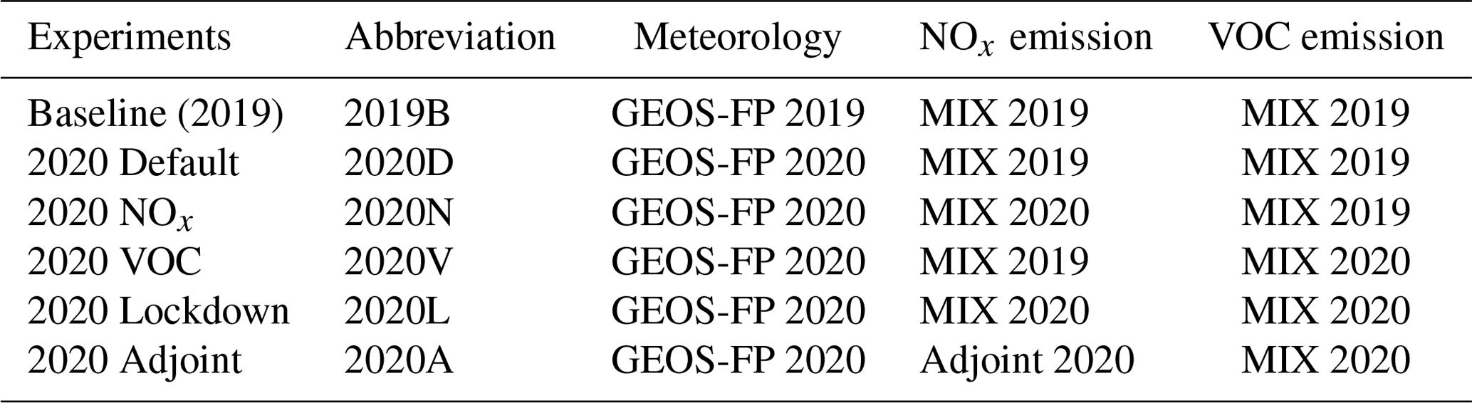
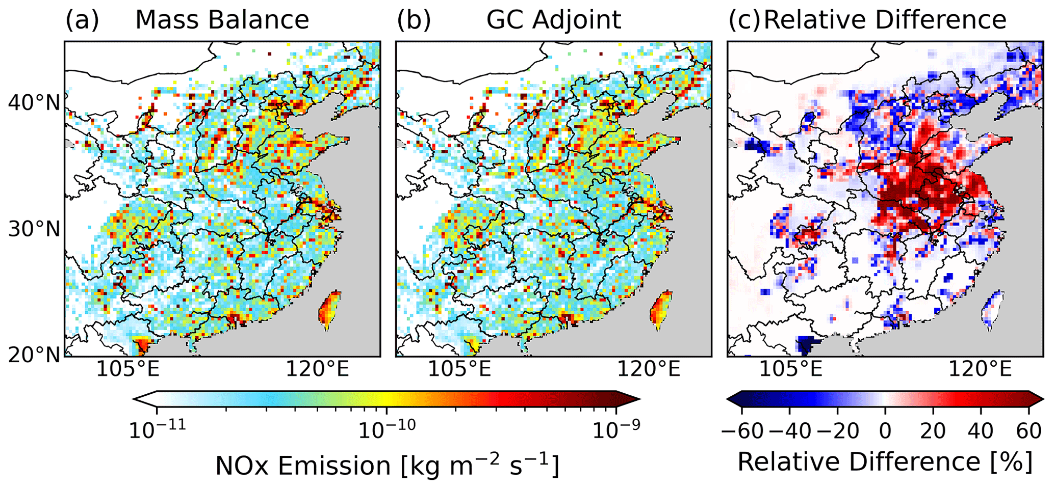
Figure 1 Updated anthropogenic NO_x emission during February–March 2020 from (a) the mass balance method and (b) the 4D-Var method as well as (c) their relative difference. The relative difference is calculated by subtracting the value in panel (a) from panel (b) and then dividing the difference by panel (a).

2.5 GEOS-Chem model experiments

A series of sensitivity experiments are conducted over China with different NO_x and VOC emissions and GEOS-FP meteorological fields in different years using the GEOS-Chem (version 12.7.2) model. All simulations are conducted from 15 January to 31 March. The 17 d before 1 February is used for spin-up, and the model outputs for February and March are used for the analysis. The configurations of different simulations are listed in Table 1.

We use the following equations to quantify the contributions from NO_x and VOC emission reductions due to COVID-19 and meteorological variations to the increase in surface O₃ as follows:

$$\begin{array}{}\text{(2)}& {\displaystyle }& {\displaystyle }\mathrm{\Delta }{\mathbf{O}}_{\mathbf{3}}^{{\mathrm{NO}}_x}={\displaystyle \frac{{\mathbf{O}}_{\mathbf{3}}^{\mathrm{2020}\mathrm{A}}-{\mathbf{O}}_{\mathbf{3}}^{\mathrm{2020}\mathrm{V}}}{{\mathbf{O}}_{\mathbf{3}}^{\mathrm{2019}\mathrm{B}}}}\times \mathrm{100}\mathit{\%},\text{(3)}& {\displaystyle }& {\displaystyle }\mathrm{\Delta }{\mathbf{O}}_{\mathbf{3}}^{\mathrm{VOC}}={\displaystyle \frac{{\mathbf{O}}_{\mathbf{3}}^{\mathrm{2020}\mathrm{L}}-{\mathbf{O}}_{\mathbf{3}}^{\mathrm{2020}\mathrm{N}}}{{\mathbf{O}}_{\mathbf{3}}^{\mathrm{2019}\mathrm{B}}}}\times \mathrm{100}\mathit{\%},\text{(4)}& {\displaystyle }& {\displaystyle }\mathrm{\Delta }{\mathbf{O}}_{\mathbf{3}}^{\mathrm{ems}}={\displaystyle \frac{{\mathbf{O}}_{\mathbf{3}}^{\mathrm{2020}\mathrm{A}}-{\mathbf{O}}_{\mathbf{3}}^{\mathrm{2020}\mathrm{D}}}{{\mathbf{O}}_{\mathbf{3}}^{\mathrm{2019}\mathrm{B}}}}\times \mathrm{100}\mathit{\%},\end{array}$$

$$\begin{array}{}\text{(5)}& \mathrm{\Delta }{\mathbf{O}}_{\mathbf{3}}^{\mathrm{met}}={\displaystyle \frac{{\mathbf{O}}_{\mathbf{3}}^{\mathrm{2020}\mathrm{D}}-{\mathbf{O}}_{\mathbf{3}}^{\mathrm{2019}\mathrm{B}}}{{\mathbf{O}}_{\mathbf{3}}^{\mathrm{2019}\mathrm{B}}}}\times \mathrm{100}\mathit{\%},\end{array}$$

where $\mathrm{\Delta }{\mathbf{O}}_{\mathbf{3}}^{{\mathrm{NO}}_x}$, $\mathrm{\Delta }{\mathbf{O}}_{\mathbf{3}}^{\mathrm{VOC}}$ and $\mathrm{\Delta }{\mathbf{O}}_{\mathbf{3}}^{\mathrm{ems}}$ are the relative differences in surface O₃ concentration caused by emission decline in NO_x, VOC, and both NO_x and VOC resulting from COVID-19. $\mathrm{\Delta }{\mathbf{O}}_{\mathbf{3}}^{\mathrm{met}}$ represents the relative contribution to the surface O₃ change from the meteorological variation between 2 years. ${\mathbf{O}}_{\mathbf{3}}^{\mathrm{2019}\mathrm{B}}$, ${\mathbf{O}}_{\mathbf{3}}^{\mathrm{2020}\mathrm{D}}$, ${\mathbf{O}}_{\mathbf{3}}^{\mathrm{2020}\mathrm{N}}$, ${\mathbf{O}}_{\mathbf{3}}^{\mathrm{2020}\mathrm{V}}$, ${\mathbf{O}}_{\mathbf{3}}^{\mathrm{2020}\mathrm{L}}$ and ${\mathbf{O}}_{\mathbf{3}}^{\mathrm{2020}\mathrm{A}}$ are mean MDA8 surface O₃ concentrations simulated by the modeling experiments Baseline (2019), 2020 Default, 2020 NO_x, 2020 VOC, 2020 Lockdown and 2020 Adjoint, respectively (Table 1).

The difference in simulated surface O₃ between 2020 and 2019 is the result of both emission reductions and meteorological variations and is denoted as $\mathrm{\Delta }{\mathbf{O}}_{\mathbf{3}}^{\mathrm{all}}$. It is calculated and evaluated against the observed relative difference in mean MDA8 O₃ in February to March between 2019 and 2020 at all ground sites as follows:

$$\begin{array}{}\text{(6)}& \mathrm{\Delta }{\mathbf{O}}_{\mathbf{3}}^{\mathrm{all}}={\displaystyle \frac{{\mathbf{O}}_{\mathbf{3}}^{\mathrm{2020}\mathrm{A}}-{\mathbf{O}}_{\mathbf{3}}^{\mathrm{2019}\mathrm{B}}}{{\mathbf{O}}_{\mathbf{3}}^{\mathrm{2019}\mathrm{B}}}}\times \mathrm{100}\mathit{\%}.\end{array}$$

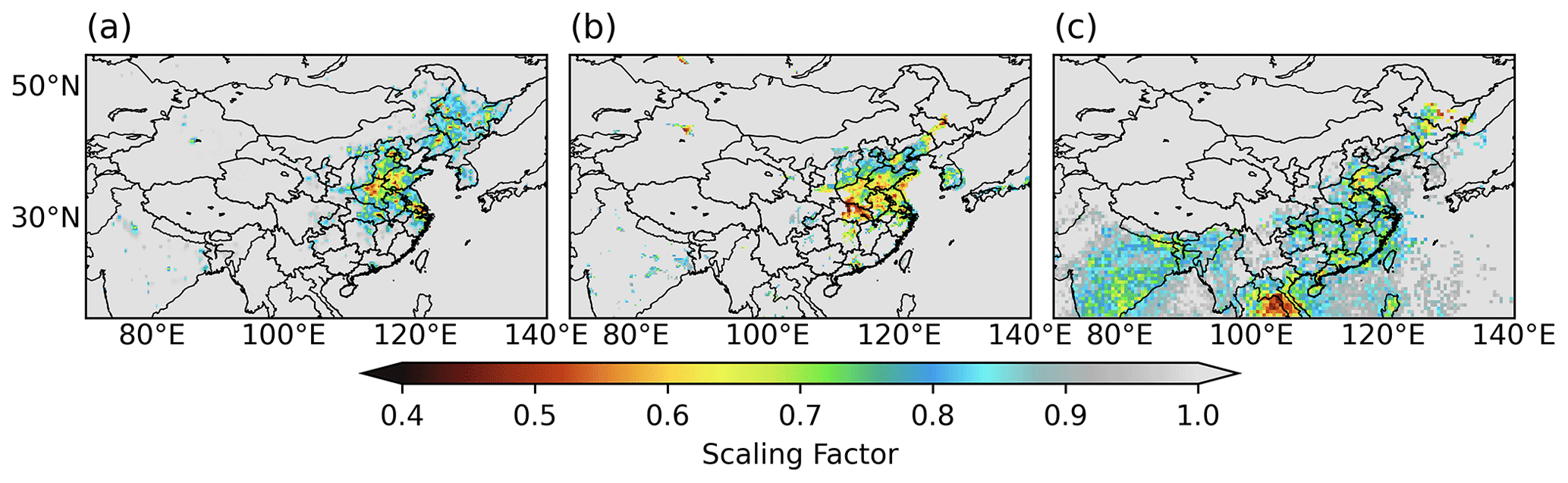
Figure 2 Scaling factors for anthropogenic NO_x emissions in February–March from 2019 to 2020 as derived from the (a) 4D-Var method and (b) mass balance method. Scaling factors for anthropogenic VOC emissions from the mass balance are shown in panel (c).

3 Results

3.1 Changes in NO_x and VOC emissions during COVID-19

We updated the anthropogenic NO_x emissions during the COVID-19 lockdown using both the 4D-Var method and mass balance method (Figs. 1 and 2). The NO_x emissions from the 4D-Var inversion share a similar spatial pattern and magnitude with those found using the mass balance method (Fig. 1). However, the NO_x emissions from the 4D-Var inversion are lower overall than those from the mass balance method over North China by ∼ 10 % and larger over central China by ∼ 40 %. Figure 2a and b show that the 4D-Var NO_x emission reduction is more severe over urban regions and displays a smoother spatial pattern than that from the mass balance approach, which is caused by the arbitrary cutoff with 0.1 DU of NO₂ VCD in the latter. Furthermore, the 4D-Var inversion captured the NO_x emission decline in northeast China where the mass balance approach did not because of the low NO₂ VCD. During February–March 2020, the anthropogenic NO_x emissions in East China decreased by ∼ 30 % compared to those in the same period in 2019.

We also scale the anthropogenic VOC emissions based on the TROPOMI HCHO data (Fig. 2c). The VOC emissions decrease by ∼ 20 %–30 % in East Asia and South Asia. The anthropogenic VOC emission changes in sparsely populated areas over northwest China are neglected. TROPOMI HCHO data cannot distinguish the anthropogenic emissions from biogenic and biomass burning sources for the Indochinese Peninsula in Southeast Asia because of the dense vegetation in this region. However, this study investigated the O₃ pollution in China; Southeast Asia, with its dense vegetation, is outside our study domain. The impact of a VOC emission bias in Southeast Asia on surface O₃ pollution in China is negligible, considering the generally short lifetime of biogenic VOC (Atkinson, 2000). For the populated urban regions in China, where the surface O₃ pollution exerts more significant health impacts, the anthropogenic source dominates the VOC emissions (Williams and Koppmann, 2007).

Figure 3 Comparison of tropospheric NO₂ VCD from (a) the TROPOMI product in February–March 2020 with that from the GEOS-Chem (b) 2020 Default simulation, (c) 2020 NO_x simulation and (d) 2020 Adjoint simulation. The pink and black circles mark the areas where NO_x emissions from 4D-Var mitigated the NO₂ overestimation by the mass balance method. The emissions and meteorology configurations are listed in Table 1 for the GEOS-Chem 2020 Default simulation, 2020 NO_x simulation and 2020 Adjoint simulation.

Figure 4 Scatterplot of TROPOMI NO₂ VCD versus the GEOS-Chem simulations for (a) Baseline (2019), (b) 2020 Default, (c) 2020 NO_x and (d) 2020 Adjoint. TROPOMI data in February–March of 2019 were used in panel (a), and those of 2020 were used in panels (b)–(d). The emissions and meteorology configurations for GEOS-Chem simulations are listed in Table 1. Only pixels larger than 0.1 DU, with TROPOMI NO₂ VCD in February–March 2019, are included in all comparisons.

3.2 Validation of NO₂ simulations

We further assess our updated anthropogenic NO_x emissions by comparing the NO₂ VCD from TROPOMI with that from GEOS-Chem with the anthropogenic NO_x emissions before and after the scaling (Figs. 3 and 4). Before updating the NO_x emissions, the 2020 Default (Fig. 3b) simulation significantly overestimates the NO₂ VCD compared to the TROPOMI NO₂ observations (Fig. 3a). With the NO_x emissions updated, the 2020 NO_x (Fig. 3c) and 2020 Adjoint (Fig. 3d) simulations exhibit a much better agreement with the TROPOMI NO₂ observation than the 2020 Default observation. However, Fig. 3c shows that the GEOS-Chem simulation with the NO_x emissions from the mass balance approach overestimated the NO₂ VCD over Beijing and the southwest Hebei Province (pink and black circles in Fig. 3) compared with TROPOMI data. The reason is that scaling factors are applied only to anthropogenic NO_x emissions, not total NO_x emissions, so it is expected that the model may still overestimate the NO₂ column after scaling part of the total NO_x emission. With the anthropogenic NO_x emissions optimized by the 4D-Var method, the overestimation of NO₂ VCD over Beijing and the southwest Hebei Province (pink and black circles in Fig. 3) is mitigated compared with the NO_x emissions from the mass balance approach.

Figure 4 further displays the statistics for the comparison between the TROPOMI NO₂ and GEOS-Chem simulations via the scatterplot. The Baseline (2019) simulation captures the magnitude of NO₂ VCD observations in 2019 well (Fig. 4a). The root mean square error (RMSE) and mean bias error (MBE) for the simulation with 2020 NO_x emissions derived from the mass balance method (Fig. 4b) decreased by 0.050 and 0.057 DU as compared to the 2020 Default (Fig. 4c) simulation. Compared with the result from the GEOS-Chem simulation 2020 NO_x, emissions from the 2020 Adjoint simulation (Fig. 4d) further led to the reduction in the MBE of the NO₂ VCD by 0.006 DU and improved the correlation coefficient by 0.003. The significant overestimation of several pixels, with the TROPOMI NO₂ VCD larger than 0.4 DU by the simulation 2020 NO_x, is also mitigated by the 2020 Adjoint simulation. The MBEs between GEOS-Chem and TROPOMI for the Baseline (2019), 2020 NO_x and 2020 Adjoint simulations are −0.004, 0.015 and 0.009 DU, respectively. The corresponding relative biases are 1.9 %, 10 % and 6.0 %, which are all less than the relative uncertainty of ∼ 30 % for the TROPOMI tropospheric NO₂ VCD over East China (Van Geffen et al., 2022). The improved agreement between the simulation with updated NO_x emission and TROPOMI NO₂ provides a basis for further analyzing the mechanism of aggravated surface O₃ pollution.

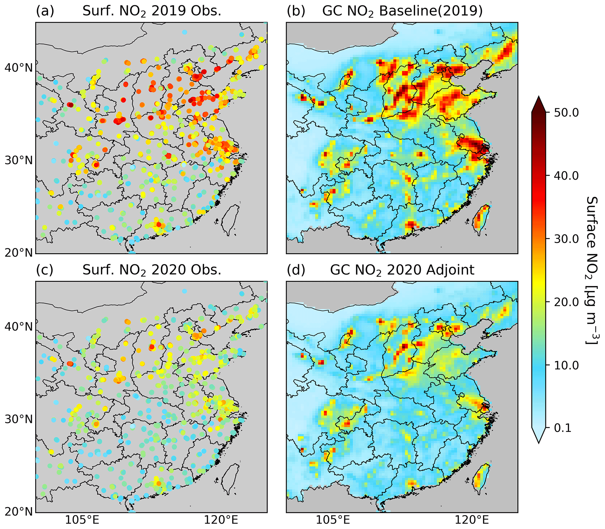
Figure 5 Comparison of surface NO₂ concentrations from ground measurements for (a) February–March 2019 and (c) February–March 2020 versus those from the GEOS-Chem (b) Baseline (2019) and (d) 2020 Adjoint simulations. Grey color means no data are presented.

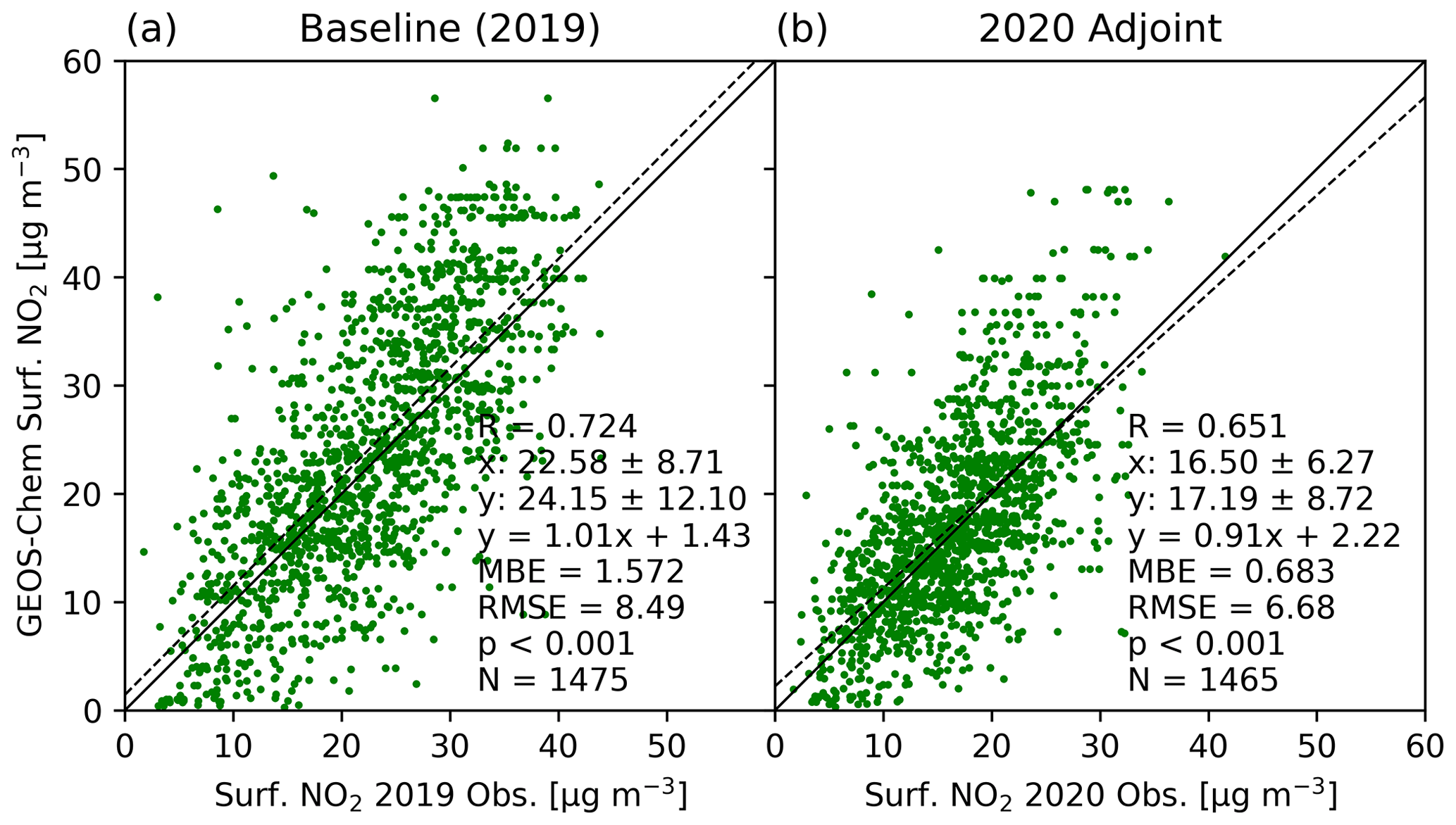
Figure 6 Scatterplots for comparing the surface NO₂ concentrations from the GEOS-Chem simulations and ground measurements. (a) The GEOS-Chem Baseline (2019) simulation versus ground measurements in February–March 2019. (b) The GEOS-Chem 2020 Adjoint simulation versus ground measurements in February–March 2020. Note that the number of ground sites differs in these 2 years.

Table 2 Evaluation statistics for modeled surface NO₂ compared with the in situ measurements.^∗

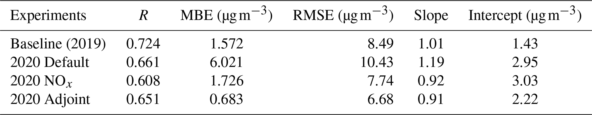
^∗ The Baseline (2019) simulation experiment is compared with the ground measurements in February–March 2019. The other three experiments are compared with the ground measurements in February–March 2020.

Figures 5 and 6 show the comparison of surface NO₂ between ground measurements and GEOS-Chem simulations. The GEOS-Chem Baseline (2019; Fig. 5b) and 2020 Adjoint (Fig. 5d) simulations capture both the spatial pattern and magnitude of surface NO₂ measurements in February–March of 2019 (Fig. 5a) and 2020 (Fig. 5c) well, respectively. Figure 6 further displays the good agreements of surface NO₂ from Baseline (2019) (Fig. 6a) and 2020 Adjoint (Fig. 6b) with the in situ measurements via scatterplots. Table 2 displays the evaluation statistics, including the correlation coefficient (R), MBE, RMSE, and the slope and intercept of the linear regression, for the simulated surface NO₂ from various simulation experiments compared with the in situ measurements. The correlation coefficient, MBE and RMSE between the Baseline (2019) simulation and the ground measurements in February–March 2019 are 0.724, 1.572 and 8.49 µg m⁻³, respectively. Without updating the NO_x emissions in 2020, the 2020 Default simulation overestimates the ground measurements of surface NO₂ in February–March 2020 (Table 2). The slope for the linear regression is 1.19, and the MBE and RMSE are 6.021 and 10.43 µg m⁻³, respectively (Table 2). After updating the NO_x emissions, the GEOS-Chem 2020 NO_x and 2020 Adjoint simulations have good agreements with the in situ measurements in February–March 2020. The correlation coefficient between the simulation 2020 Adjoint and the in situ measurements is 0.651, which is higher than that of 0.608 for the simulation 2020 NO_x versus the ground measurements (Table 2). The MBE and RMSE of 2020 Adjoint (0.683 and 6.68 µg m⁻³) are lower than those of 2020 NO_x (1.726 and 7.74 µg m⁻³; Table 2). This result further indicates the superiority of 4D-Var for optimizing NO_x emissions compared with the mass balance method (Cooper et al., 2017; Streets et al., 2013).

Figure 7 Taylor diagram for evaluating the GEOS-Chem simulations of (a) surface NO₂ and (b) surface O₃ during the lockdown period (February–March 2020) using ground observations for different simulation experiments listed in Table 1. The evaluation of surface O₃ only includes the areas where the NO_x emissions, optimized by 4D-Var, reduced by more than 10 %.

Figure 7a is the Taylor diagram for evaluating the GEOS-Chem simulations of surface NO₂ concentrations from the 2020 Default, 2020 NO_x and 2020 Adjoint simulations using the in situ measurements. The 2020 Adjoint simulation (inverted triangle in Fig. 7a) has the best performance among these three simulations with the lowest relative bias and lowest normalized centered RMSE. Without updating the NO_x emission, the 2020 Default simulation features a relative bias of ∼ 37 %. After updating the NO_x emissions, the 2020 NO_x simulation reduces the relative bias, the normalized centered RMSE and the normalized standard deviation from around 37 %, 1.38 and 1.80 to around 10 %, 1.20 and 1.51 compared with the 2020 Default simulation, but the correlation coefficient also decreases. Using the 4D-Var method, the 2020 Adjoint simulation further reduces the relative bias, normalized centered RMSE and normalized standard deviation and increases the correlation coefficient compared with the 2020 NO_x simulation. We also validated the VOC emissions by comparing the simulated HCHO VCD with TROPOMI measurements (Appendix D).

3.3 Evaluation of surface O₃ simulations

We evaluated the GEOS-Chem simulations of MDA8 surface O₃ from different simulation experiments listed in Table 1 using ground measurements. Figure 7b is the Taylor diagram for comparing the surface O₃ concentrations during February–March 2020 from the ground measurements and GEOS-Chem simulations. We focused on areas with significant NO_x emissions reduction to better assess the role of updated NO_x emissions in improving surface O₃ simulations. The ground sites are excluded where the NO_x emissions from 4D-Var decline by less than 10 %. The correlation coefficient between the Baseline (2019) simulation and ground observations is ∼ 0.53, and the relative bias is around −25 %. By applying 2020 meteorological fields and scaling the VOC emissions, the correlation coefficients decreased to ∼ 0.40 for model 2020 Default and 2020 VOC simulations, with little reduction in the relative bias. By updating the NO_x emissions, the relative bias reduced to around −10 %, while the correlation coefficients remained at ∼ 0.50 for model simulations 2020 NO_x, 2020 Lockdown and 2020 Adjoint. This indicates that the NO_x emission updates significantly improve the surface O₃ simulations. Comparing the simulations 2020 Default and 2020 VOC, or 2020 NO_x and 2020 Lockdown, the results show that scaling VOC emissions does not improve the surface O₃ simulations significantly over continental China; however, over South China, the VOC emissions update reduces the relative bias by 3 %. Among all simulations, 2020 Adjoint exhibits the best performance with the lowest normalized centered RMSE, the largest correlation coefficient and a low relative bias of ∼ 10 %. This result further confirms the superiority of the 4D-Var with respect to the mass balance method for optimizing NO_x emissions. Therefore, we used the 2020 Adjoint to evaluate the impacts of NO_x emission on surface O₃ in the following analysis.

Figure 8 Comparison of MDA8 surface O₃ in 2019 and February–March 2020 and the relative difference between 2 years from the GEOS-Chem model simulations (a–c) versus ground observations (d–f). Also shown is the GEOS-Chem mean MDA8 O₃ at 9 $\mathrm{m}\mathrm{a}.\mathrm{s}.\mathrm{l}.$ under standard temperature and pressure (STP; 273.15 K and 101.325 kPa) from the (a) Baseline (2019) and (b) 2020 Adjoint simulations (Table 1) together with (c) their relative difference. Ground observed mean MDA8 surface O₃ under STP in (d) February–March 2019 and (e) February–March 2020 with (f) their relative difference. The pink and green boxes in panel (c) and panel (f) define the North China and South China domain.

Figure 8 compares the modeled surface O₃ in February–March of 2019 (Fig. 8a) and 2020 (Fig. 8b) and the relative difference (Fig. 8c) computed from Eq. (6) with the in situ measurements (Fig. 8d–f). The ground observations show that the highest level of surface O₃ pollution occurs in North China and in the southwest of China. The average MDA8 O₃ in 2 months can reach up to ∼ 110 µg m⁻³ at STP (∼ 51.4 ppbv), which is higher than the China National Ambient Air Quality Standard daily maximum 8 h grade I standard of 100 µg m⁻³. The GEOS-Chem model underestimates the surface O₃ over North China for both years compared with ground observations, which could be a result of the underestimation of biogenic VOC emissions (Appendix D). The underestimation of the simulated O₃ over North China does not significantly affect our study purpose since this study focuses on revealing the impacts of emissions and meteorology change on the surface O₃ change by each region. The bias is predominantly systematic and was substantially canceled when we computed the relative difference in the surface O₃. The model captures well the magnitude and spatial distribution of surface O₃ and the increasing trend in South China. In South China, the measured surface O₃ in February–March 2020 increases by 30 %–50 %, while over North China, it increases generally by less than 20 % and even decreases in some regions. The relative differences in simulated surface O₃ between 2 years is comparable to the ground observations over South China (green box in Fig. 8c and f). In the Sichuan Basin, the trend of the surface O₃ change from the model is opposite to that of the measurements, which is probably caused by the inaccurate simulation of the meteorological effects (see Sect. 3.4) due to the complex terrain features in this region. The localized improvement of the model simulation is further needed for the regional study. Over North China (pink box in Fig. 8c and f), the average relative differences between 2 years from the model and observation are 4.27 % and −3.01 %, respectively, both of which are much smaller than their counterparts in South China. While the relative difference from model simulations has different signs as compared to that of observations on average, the change in O₃ is indeed small and the model is able to capture the part of O₃ decrease in the southwest part of the North China domain (Fig. 8c). We note that some previous studies showed a large increase in O₃ in North China, but such an increase is in comparison with the O₃ in the month right before the lockdown (not the same time in 2019; Shi and Brasseur, 2020; Liu et al., 2021).

Figure 9 Relative difference in simulated surface O₃ caused by (a) NO_x emission reduction, (b) VOC emission reduction, (c) overall emission reduction and (d) meteorological variations due to the COVID-19 lockdown. The pink and green boxes in each panel define the North China and South China domain.

3.4 Relative contribution from declining emissions and meteorological variations

Using Eqs. (2)–(5), we can analyze the mechanism of surface O₃ increase in China during the COVID-19 pandemic (Fig. 9). NO_x emission reduction as a result of the COVID-19 lockdown leads to a ∼ 8 % increase in the mean MDA8 surface O₃ over North China (pink boxes in Fig. 9) between 2019 and February–March 2020 (Fig. 9a), while the VOC emission decline causes ∼ 3 % of O₃ decrease (Fig. 9b). The average contribution of the meteorological variations to the surface O₃ change is less than 1 % in North China (Fig. 9d). However, in South China, the inter-annual meteorological variations dominate the surface O₃ increases, causing a ∼ 30 % increase (Fig. 9d), while the reduction in NO_x and VOC emissions has little impact. The overall magnitude of emissions contribution to the surface O₃ change over North China is ∼ 5 %, which is similar to that of the meteorological effects, but meteorological variations lead to both O₃ increases and decreases in different regions. Over South China, the meteorological effect is much larger than the net effects of declining emissions. Overall, the impact of inter-annual meteorological variations between 2019 and 2020 is almost 30 times larger than the overall emissions impacts on the aggregated surface O₃ pollution in China.

Our results are consistent with the conclusion from Zhao et al. (2020) that states that the meteorological variations have larger impacts than emissions reduction on surface O₃ in the southern city of Guangzhou, but in Beijing, emission reduction has a larger impact during 23–29 January. Wang et al. (2022) also showed that ∼ 80 % of the O₃ MDA8 increase during the COVID-19 lockdown period is caused by the meteorological factors and that ∼ 20 % is caused by the emission decline in East China. T. Liu et al. (2020) reported that the surface O₃ increase in the major cites of the Yangtze River Delta region was driven by both emission reduction and meteorological variations to a similar degree from the pre-lockdown period (1–22 January 2020) to the lockdown period (23 January–29 February 2020). However, Zhao et al. (2020), Wang et al. (2022) and T. Liu et al. (2020) only focused on the lockdown period of 1 to 5 weeks in reference to the time period right before the lockdown instead of the same period in previous years, which did not provide a comprehensive analysis over the whole lockdown period, and Zhao et al. (2020) and T. Liu et al. (2020) did not separate the effects of the seasonal trend from the meteorological anomalies. Moreover, T. Liu et al. (2020) and Wang et al. (2022) only analyzed four representative cities of the East China region instead of showing the analysis at a national scale. Further, Zhao et al. (2020) did not update the anthropogenic emissions during the lockdown period, which brings significant uncertainties into their analysis. Previous studies found that the TROPOMI NO₂ product has a negative bias of −7 % to −20 % (Verhoelst et al., 2021; Judd et al., 2020; Li et al., 2021). The sensitivity simulations indicate that this low bias does not significantly affect the model evaluation and our main conclusions (figures not shown).

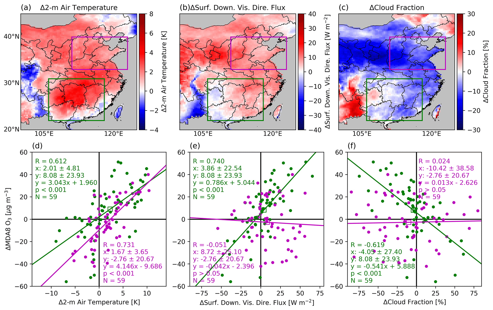
Figure 10 The changes in (a) the 2 m air temperature, (b) the downward visible direct flux at the surface and (c) the cloud fraction from February–March 2019 to February–March 2020. Scatterplots between the daily difference in surface O₃ measurements and (d) the 2 m air temperature, (e) the downward visible direct flux at the surface and (f) the cloud fraction in February–March between 2020 and 2019 over South China (green dots) and North China (pink dots). The green and pink open squares in (d–f) mark the predicted average change in surface MDA8 O₃ in South China and North China, respectively, based on the linear regression against the change in meteorological variables.

3.5 Critical meteorological variables causing aggravated surface O₃ pollution in South China

To identify the critical meteorological variables that led to the aggravated surface O₃ pollution in South China, we investigated the correlations between the surface O₃ concentrations and 2 m air temperature, downward visible direct flux at the surface, cloud fraction, relative humidity, and wind speed. The positive correlation between the surface O₃ and temperature is widely observed and reported in the literature (Pusede et al., 2015). A higher temperature leads to higher concentrations of surface O₃ because it improves the O₃ production rate by affecting the organic reactivity, production of HO_x radicals, and the formation and decomposition of peroxy nitrates and alkyl nitrates (Pusede et al., 2015). We calculated the daily difference in February–March between 2020 and 2019 (excluding 29 February 2020) for the daily mean of MDA8 O₃ from ground measurements and 2 m air temperature and the downward visible direct flux at the surface and cloud fraction from GEOS-FP data used in our GEOS-Chem simulations for South China (22–31° N, 106–118° E; green box in Fig. 10a–c) and North China (33–40° N, 111–123° E; pink box in Fig. 10a–c). Figure 10 displays the difference in the 2-month mean 2 m air temperature (Fig. 10a), downward visible direct flux at the surface (Fig. 10b) and cloud fraction (Fig. 10c) in February–March between 2020 and 2019 as well as the scatterplot between the daily difference in measured surface O₃ concentration and 2 m air temperature (Fig. 10d), downward visible direct flux at the surface (Fig. 10e) and cloud fraction (Fig. 10f) over both South China (green dots in Fig. 10d–f) and North China (pink dots in Fig. 10d–f). We found that the 2 m air temperature increased by ∼ 2.3 °C in South China and that the daily differences in surface O₃ concentration and 2 m air temperature are well correlated, with a positive correlation coefficient of 0.612. Therefore, the temperature increase contributed to the significant aggravated surface O₃ pollution in South China. The enhanced solar radiation at the surface could also promote the production of O₃ via photochemical reactions. The correlation coefficient between the daily difference in surface O₃ concentration and downward visible direct flux at the surface is as high as 0.740 in South China (Fig. 10e). The reason for the increase in temperature and solar radiation at the surface is the lower cloud fraction. By analyzing the GEOS-FP data, we found the cloud fraction decreased by ∼ 5 % (Fig. 10c), and the downward visible direct flux at the surface increased by 5 W m⁻² (Fig. 10b) over South China. The lower cloud fraction increases the downward solar radiation at the surface during the lockdown period, leading to a higher surface air temperature. The change in cloud fraction is negatively correlated with the change in surface O₃ in South China, with a correlation coefficient of −0.619 (Fig. 10f).

Figure 11 Same as Fig. 10 but for (a, c) relative humidity and (b, d) wind speed.

In North China, the 2 m air temperature also increased by 1.8 ° C, but the measured surface MDA8 O₃ decreased by 3 % (Fig. 8f). Figure 10d shows the daily difference in MDA8 O₃, and the 2 m air temperature over North China also has a high correlation coefficient of 0.731. However, the intercept of the linear regression line is negative, indicating that surface O₃ could decrease even though the temperature increases. This negative intercept is caused by the net effects of factors, other than temperature, including chemistry, emissions and other meteorological factors. It is a challenge to quantify the contributions of each individual factor because these factors are thermodynamically or dynamically related. The predicted average changes in surface MDA8 O₃ in South China and North China are marked by the open green and pink squares, respectively, in Fig. 10d based on the linear regression. Because of the different intercepts, the predicted MDA8 O₃ in South China increases by ∼ 9.0 µg m⁻³, while it decreases by 2.2 µg m⁻³ in North China, although the average temperature increased in both South and North China. Contrary to South China, the change in solar radiation at the surface and cloud fractions is poorly correlated with the change in surface O₃ concentrations in North China (Fig. 10e and f), mainly due to a more important role of emission change in regulating the surface O₃ in North China.

The impacts of relative humidity and wind speed on the surface O₃ change are also investigated (Fig. 11). The relative humidity increased, on average, by ∼ 5.1 % in North China and decreased by ∼ 3.0 % in South China. The strong correlation (R = −0.675) between the change in relative humidity and surface O₃ in South China indicates that the decrease in relative humidity also contributes to the increase in surface O₃ pollution in South China, but the correlation between them in North China is very low. The wind speed also changed in opposite directions in South China and North China, but we cannot identify any significant impact of wind speed on the surface O₃ pollution since the correlation coefficients are low in both South China and North China. In summary, the significant increase in surface O₃ pollution during the lockdown period in South China could be primarily attributed to the higher temperature, enhanced solar radiation at the surface and decreased relative humidity.

4 Summary

A significant reduction in primary air pollutants has been identified by surface and satellite observations during the COVID-19 pandemic in China (Bauwens et al., 2020; Miyazaki et al., 2020), which is in contrast to the increase in surface O₃. In this study, we analyzed the reasons for the enhanced surface O₃ pollution from two perspectives: anthropogenic emissions reduction and inter-annual meteorological variations. We constrain the NO_x emissions based on the TROPOMI NO₂ product using both the mass balance and 4D-Var methods. The VOC emissions were also updated based on the TROPOMI HCHO product via the mass balance approach. We analyzed the contributions from emissions reduction and meteorological variations to surface O₃ increases through a series of sensitivity simulations using the GEOS-Chem model.

The updated NO_x emissions from the 4D-Var and mass balance approaches share a similar spatial pattern. However, the NO_x emissions from 4D-Var are lower than those from the mass balance method over North China by ∼ 10 % but larger over central China by ∼ 40 %. The evaluation of the simulations with the updated emissions against the TROPOMI NO₂, in situ measurements of surface NO₂ and O₃ indicates that the NO_x emissions from the 4D-Var inversion leads to better model performance than that from the mass balance approach. The updated anthropogenic VOC emissions using the mass balance method are evaluated by comparing the GEOS-Chem HCHO and TROPOMI HCHO. However, the updated VOC emissions may still suffer from large uncertainties because of the low retrieval accuracy of TROPOMI HCHO (Vigouroux et al., 2020), large biogenic sources of VOC emissions and limited representativeness of HCHO for the whole VOC species.

The anthropogenic NO_x emission decreased by ∼ 30 % over East China during February–March 2020 compared to the same period in 2019. Over North China, NO_x emission reduction leads to a ∼ 8 % increase in the mean MDA8 surface O₃, while the VOC emissions decline causes O₃ to decrease by ∼ 3 %. The average contribution of meteorological variations to the surface O₃ change is less than 1 % in North China. However, in South China, the inter-annual meteorological variation dominates the surface O₃ increase, causing a ∼ 30 % increase, while the NO_x and VOC emission reduction has nearly no impact on O₃. Overall, the impact of inter-annual meteorological variations between 2019 and 2020 is almost 30 times larger than the impact of emissions on the enhanced surface O₃ pollution in China.

The significant increase in surface O₃ in South China could be attributed to the higher temperature, enhanced solar radiation at the surface and decreased relative humidity during the lockdown period. The lower cloud fraction increases the downward solar radiation at the surface during the lockdown period, leading to a higher surface air temperature. We cannot identify any significant impact of wind speed on the surface O₃ pollution.

Appendix A: NO_x emission reduction in China from 2010 to 2019

The default anthropogenic NO_x emission over East Asia in GEOS-Chem is MIX 2010 (Li et al., 2017). To generate the anthropogenic NO_x emission in 2019, we calculated the ratio of mean TROPOMI tropospheric NO₂ VCD in February–March 2019 to GEOS-Chem simulated NO₂ VCD with the default MIX 2010 emission as the scaling factor (Fig.  A1). The scaling factors in regions where mean TROPOMI tropospheric NO₂ VCD in February–March 2019 is less than 0.1 DU are set to 1. From 2010 to 2019, the anthropogenic NO_x emission has declined significantly as a result of the clean air actions of the Chinese government (Zheng et al., 2018).

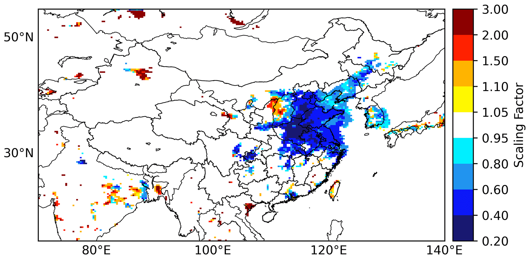
Figure A1 The scaling factor of anthropogenic NO_x emissions from year 2010 to 2019.

Appendix B: Applying the TROPOMI NO₂ averaging kernel in the observation operator

To optimize the NO_x emissions and minimize the cost function (Eq. 1) with the 4D-Var method, the GEOS-Chem adjoint needs to compute the derivative of the cost function with respect to the model parameters to be optimized, which are the scaling factors of the anthropogenic NO_x emissions in this study. An essential step is to calculate the adjoint forcing F, which is the derivative of the cost function with respect to the modeled NO₂ concentration shown as Eq. (B1):

$$\begin{array}{}\text{(B1)}& \mathit{F}={\displaystyle \frac{\partial J}{\partial \mathit{c}}}={\mathbf{S}}_{\text{obs}}^{-\mathrm{1}}\left[H\right(\mathit{c})-\mathit{s}]{\displaystyle \frac{\partial H\left(\mathit{c}\right)}{\partial \mathit{c}}}.\end{array}$$

For each single TROPOMI NO₂ observation, the adjoint forcing component f and cost function component j are computed as Eqs. (B2) and (B3):

$$\begin{array}{}\text{(B2)}& {\displaystyle }& {\displaystyle }f={\displaystyle \frac{M_{\text{gc}}{v}_{\text{gc}}-M_{\text{obs}}{v}_{\text{obs}}}{e_{\text{obs}}{M}_{\text{obs}}}}{M}_{\text{gc}},\text{(B3)}& {\displaystyle }& {\displaystyle }j={\displaystyle \frac{\mathrm{0.5}f(M_{\text{gc}}{v}_{\text{gc}}-M_{\text{obs}}{v}_{\text{obs}})}{M_{\text{gc}}}}.\end{array}$$

Here, M_gc is the GEOS-Chem air mass factor applying the GEOS-Chem NO₂ vertical profiles and TROPOMI NO₂ averaging kernel. M_obs is the TROPOMI air mass factor. v_gc and v_obs are the tropospheric NO₂ VCD from the GEOS-Chem model and TROPOMI observation, respectively. The product of the air mass factor and NO₂ VCD is the NO₂ slant column density. e_obs is the standard error in the TROPOMI tropospheric NO₂ VCD.

We calculated the GEOS-Chem air mass factor M_gc as Eq. (B4) following Qu et al. (2019).

$$\begin{array}{}\text{(B4)}& M_{\text{gc}}={\displaystyle \frac{{\sum }_{i\in \text{trop.}}{c}_i^{\text{gc}}\mathrm{\Delta }{p}_i^{\text{gc}}{w}_i^{\text{gc}}}{{\sum }_{i\in \text{trop.}}{c}_i^{\text{gc}}\mathrm{\Delta }{p}_i^{\text{gc}}}}\end{array}$$

Here, $c_i^{\text{gc}}$ is the GEOS-Chem NO₂ mixing ratio at the vertical layer i and $\mathrm{\Delta }{p}_i^{\text{gc}}$ is the pressure difference between the GEOS-Chem vertical layer i and i+1. $w_i^{\text{gc}}$ is the scattering weight at the GEOS-Chem vertical layer i, which is calculated by the linear interpolation of the scattering weights at the vertical coordinate of the model TM5 used for the TROPOMI NO₂ retrieval. The scattering weight at the TM5 vertical layer l ($w_{\mathrm{l}}^{\text{TM5}}$) is computed as the product of the TROPOMI air mass factor and the TROPOMI averaging kernel at the TM5 vertical layer l ($A_{\mathrm{l}}^{\text{TM5}}$) using Eqs. (B5) and (B6) (Eskes and Boersma, 2003; Palmer et al., 2001):

$$\begin{array}{}\text{(B5)}& {\displaystyle }& {\displaystyle }{w}_l^{TM\mathrm{5}}={\displaystyle \frac{M_{\text{obs}}{A}_l^{TM\mathrm{5}}}{M_{\text{geo}}}},\text{(B6)}& {\displaystyle }& {\displaystyle }{M}_{\text{geo}}=\sec {\mathit{\theta }}_{\mathrm{0}}+\sec \mathit{\theta },\end{array}$$

where M_geo is the geometric air mass factor and θ₀ and θ are the solar zenith angle and viewing zenith angle, respectively.

Appendix C: Validation of the TROPOMI NO₂ observation operator

We validated the observation operator by comparing the sensitivity of the cost function with respect to the emission scaling factor from GEOS-Chem adjoint and a finite difference estimation as shown in Eq. (C1). We shut down the transport and excluded a priori the term from the cost function for the validation so that the gradient of the cost function component in each grid cell to the local emission scaling factor equals the gradient of total cost function to the emission scaling factor in the same grid cell.

$$\begin{array}{}\text{(C1)}& {\displaystyle \frac{\partial J\left(\ln \mathit{\sigma }\right)}{\partial \ln \mathit{\sigma }}}\approx {\displaystyle \frac{J\left(\ln \right(\mathit{\sigma }+\mathrm{0.05}\left)\right)-J\left(\ln \right(\mathit{\sigma }-\mathrm{0.05}\left)\right)}{\ln (\mathit{\sigma }+\mathrm{0.05})-\ln (\mathit{\sigma }-\mathrm{0.05})}}\end{array}$$

Figure C1 compares the cost function sensitivities calculated from the GEOS-Chem adjoint and the finite difference method for the nested grids with the spatial resolution of 0.25° × 0.3125°. The spatial pattern and the magnitude of the cost function sensitivities from the two methods match with each other, with a correlation coefficient of 0.97. The statistics show that the agreement between the adjoint sensitivities and finite difference sensitivities in this study is comparable to that in Wang et al. (2020a), although we constrain the NO_x emission at a much finer resolution of 0.25° × 0.3125° than in their study (2° × 2.5°).

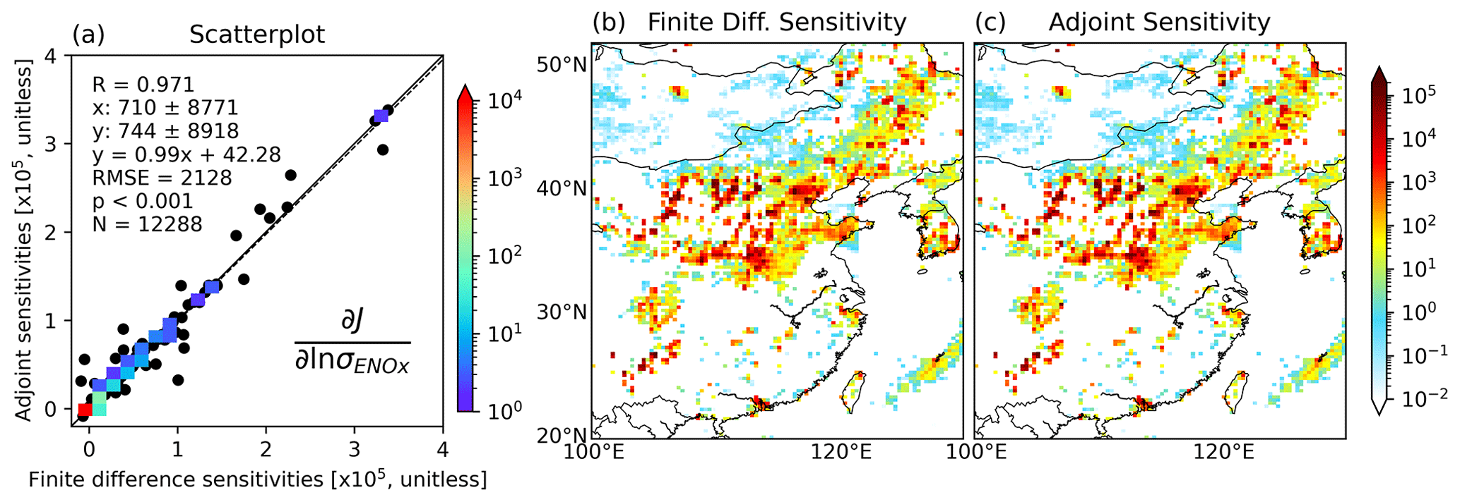
Figure C1 Comparison of adjoint sensitivities and finite difference sensitivities. (a) Scatterplot of the adjoint sensitivity of the cost function with respect to the logarithm of the NO_x emission scaling factor versus the finite difference sensitivities. The color scheme for panel (a) encodes the number of samples (the legend on the right of panel (a)). (b) Map of finite difference sensitivity. (c) Map of adjoint sensitivity.

Appendix D: Validation of HCHO simulations

It is not practical to validate the VOC emissions species by species in this study. We compare the GEOS-Chem simulation of HCHO with TROPOMI data for a rough validation of the VOC emissions. Overall, the GEOS-Chem Baseline (2019) and 2020 Adjoint simulations agree well with TROPOMI HCHO in February–March of 2019 and 2020, respectively (Fig. D1). The correlation coefficients for the two comparisons are 0.878 and 0.874, and the MBEs are −0.036 and −0.042 DU, respectively. This good agreement also supports our assumption of ignoring the change in VOC emissions from 2010 to 2019, since the anthropogenic VOC emission used for Baseline (2019) is equivalent to MIX 2010. However, Fig. D1 shows that GEOS-Chem tends to overestimate the HCHO VCD over urban regions and underestimate it over rural regions, which indicates the partition of total emissions may overestimate the anthropogenic emissions and underestimate the biogenic emissions, at least for HCHO. A more comprehensive evaluation for various species and emission sectors would be helpful for further improvement of the VOC emissions used in the model.

Figure D1 Comparison of tropospheric HCHO VCD from TROPOMI and GEOS-Chem. (a) TROPOMI HCHO in February–March 2019. (b) GEOS-Chem HCHO from Baseline (2019). (c) Scatterplot between panel (a) and panel (b). (d) TROPOMI HCHO in February–March 2020. (e) GEOS-Chem HCHO from 2020 Adjoint. (f) Scatterplot between panel (d) and panel (e). The emissions and meteorology configurations for the GEOS-Chem Baseline (2019) and 2020 Adjoint simulations are listed in Table 1.