the Creative Commons Attribution 4.0 License.
the Creative Commons Attribution 4.0 License.
 | 05 Jul 2024
A lightweight NO2-to-NOx conversion model for quantifying NOx emissions of point sources from NO2 satellite observations
Erik F. M. Koene
Maarten Krol
Dominik Brunner
Alexander Damm
Nitrogen oxides (NOx = NO + NO2) are air pollutants which are co-emitted with CO2 during high-temperature combustion processes. Monitoring NOx emissions is crucial for assessing air quality and for providing proxy estimates of CO2 emissions. Satellite observations, such as those from the TROPOspheric Monitoring Instrument (TROPOMI) on board the Sentinel-5P satellite, provide global coverage at high temporal resolution. However, satellites measure only NO2, necessitating a conversion to NOx. Previous studies have applied a constant NO2-to-NOx conversion factor. In this paper, we develop a more realistic model for NO2-to-NOx conversion and apply it to TROPOMI data of 2020 and 2021. To achieve this, we analysed plume-resolving simulations from the MicroHH large-eddy simulation model with chemistry for the Bełchatów (PL), Jänschwalde (DE), Matimba (ZA) and Medupi (ZA) power plants, as well as a metallurgical plant in Lipetsk (RU). We used the cross-sectional flux method to calculate NO, NO2 and NOx line densities from simulated NO and NO2 columns and derived NO2-to-NOx conversion factors as a function of the time since emission. Since the method of converting NO2 to NOx presented in this paper assumes steady-state conditions and that the conversion factors can be modelled by a negative exponential function, we validated the conversion factors using the same MicroHH data. Finally, we applied the derived conversion factors to TROPOMI NO2 observations of the same sources. The validation of the NO2-to-NOx conversion factors shows that they can account for the NOx chemistry in plumes, in particular for the conversion between NO and NO2 near the source and for the chemical loss of NOx further downstream. When applying these time-since-emission-dependent conversion factors, biases in NOx emissions estimated from TROPOMI NO2 images are greatly reduced from between −50 % and −42 % to between only −9.5 % and −0.5 % in comparison with reported emissions. Single-overpass estimates can be quantified with an uncertainty of 20 %–27 %, while annual NOx emission estimates have uncertainties in the range of 4 %–21 % but are highly dependent on the number of successful retrievals. Although more simulations covering a wider range of meteorological and trace gas background conditions will be needed to generalise the approach, this study marks an important step towards a consistent, uniform, high-resolution and near-real-time estimation of NOx emissions – especially with regard to upcoming NO2-monitoring satellites such as Sentinel-4, Sentinel-5 and CO2M.
- Article
(4384 KB) - Full-text XML
-
Supplement
(3369 KB) - BibTeX
- EndNote


Nitrogen oxides (NOx = NO + NO2) are reactive trace gases and important air pollutants since they cause oxidative stress when respired, are involved in the formation of ground-level ozone (O3) and particulate matter, and contribute to acid rain (Thurston, 2017). As most NOx emissions originate from high-temperature combustion processes, monitoring these sources is crucial for air quality regulation and can be used to estimate the (co-emitted) CO2 emissions, provided that one knows the CO2:NOx emission ratio for a given source (e.g. Goldberg et al., 2019a; Kuhlmann et al., 2021; Liu et al., 2020; Reuter et al., 2019; Hakkarainen et al., 2023). Estimating CO2 emissions from large sources such as power plants and cities will be an important component of the CO2 Monitoring and Verification Support (CO2MVS) service that is currently being developed under the European Copernicus CO2 project (CoCO2) in support of the Paris Agreement (Pinty et al., 2017; Janssens-Maenhout et al., 2020). For this purpose, emission data should be available in near-real time. A convenient method to obtain such high-resolution, uniform, consistent emission estimates is to use satellite observations (Pinty et al., 2017).
Several case studies have investigated the potential and limitations of quantifying point source CO2 emissions from space (e.g. Bovensmann et al., 2010; Goldberg et al., 2019b; Kuhlmann et al., 2021; Nassar et al., 2017; Reuter et al., 2019). One of the methods to quantify emissions is the cross-sectional flux method, which determines emissions by dividing a plume into several cross-sections. By integrating the measured vertical column densities along a cross-section, a line density is obtained. Each line density can be converted into a flux by multiplication by an effective wind speed representing the mean transport speed of the plume. Under the assumption of steady-state conditions, the flux at each cross-section along the plume can be used to estimate the emissions (Varon et al., 2018).
Estimating CO2 emissions from NO2 satellite data is appealing because local NO2 enhancements can be measured with higher accuracy than for CO2. There are also a number of existing and upcoming satellites that provide NO2 products with high temporal and spatial coverage in comparison with CO2 satellites. The most prominent existing instrument is the TROPOspheric Monitoring Instrument (TROPOMI) on the Sentinel-5 Precursor satellite, which provides daily observations of NO2 and other trace gases with a spatial resolution of 3.5 km × 5.5 km at nadir (van Geffen et al., 2022; Veefkind et al., 2012). Several case studies have shown that TROPOMI data can be used to estimate NOx emissions from cities and power plants (e.g. Douros et al., 2023; Goldberg et al., 2019b; Lorente et al., 2019).
Satellite-based radiance data only allow for the retrieval of NO2 but not NO. However, more than 90 % of NOx from combustion processes is emitted as NO, which is then partially oxidised to NO2 inside the plume (Pronobis, 2020; Seinfeld and Pandis, 2016). To retrieve NOx emissions, it is therefore necessary to convert the measured NO2 quantities to NOx. Previous studies have often used a constant NO2-to-NOx conversion factor of about 1.32, derived assuming steady-state conditions (e.g. Beirle et al., 2011, 2021; de Foy et al., 2015; Kuhlmann et al., 2021). Recent studies that used regional chemistry transport model simulations derived spatially varying conversion factors in the range of 1.1 to 1.9 but acknowledged that the values near sources are likely larger (e.g. Lorente et al., 2019; Rey-Pommier et al., 2022; Goldberg et al., 2022; Lange et al., 2022; Hakkarainen et al., 2024).
To study the NO2-to-NOx conversion factor inside plumes, plume-resolving large-eddy simulations of atmospheric transport with chemistry are necessary. In the CoCO2 project such simulations were conducted using the MicroHH model (van Heerwaarden et al., 2017; Krol et al., 2024). These simulations are described in further detail in Sect. 2.1.2. Krol et al. (2024) showed that the NOx:NO2 ratios inside the plume are the highest near the source and decrease roughly exponentially with increasing time after emission. Figure 1 schematically depicts the evolution of NO, NO2 and NOx concentrations in a plume. While more than 90 % of NOx is emitted as NO (Pronobis, 2020), it is rapidly oxidised to NO2 in the presence of ozone (O3), titrating the available O3. The concentration of O3 starts to increase again only after dilution and mixing of the plume with ambient air along the plume, leading to further oxidation of NO. As a result, the ratio of NOx to NO2 is the largest shortly after the emission and gradually decreases over time. The rate of this oxidation process depends on several factors, such as the amount of NOx emitted, the concentration of O3 and volatile organic compounds (VOCs), photolysis rates, and meteorological conditions. Subsequently, NO2 is mainly removed by reacting with OH radicals with lifetimes ranging from hours to a few days in the lower troposphere (Seinfeld and Pandis, 2016). According to Fig. 1, NOx decays exponentially with a constant e-folding lifetime, but in reality the lifetime may change along the plume due to changing OH radical concentrations.
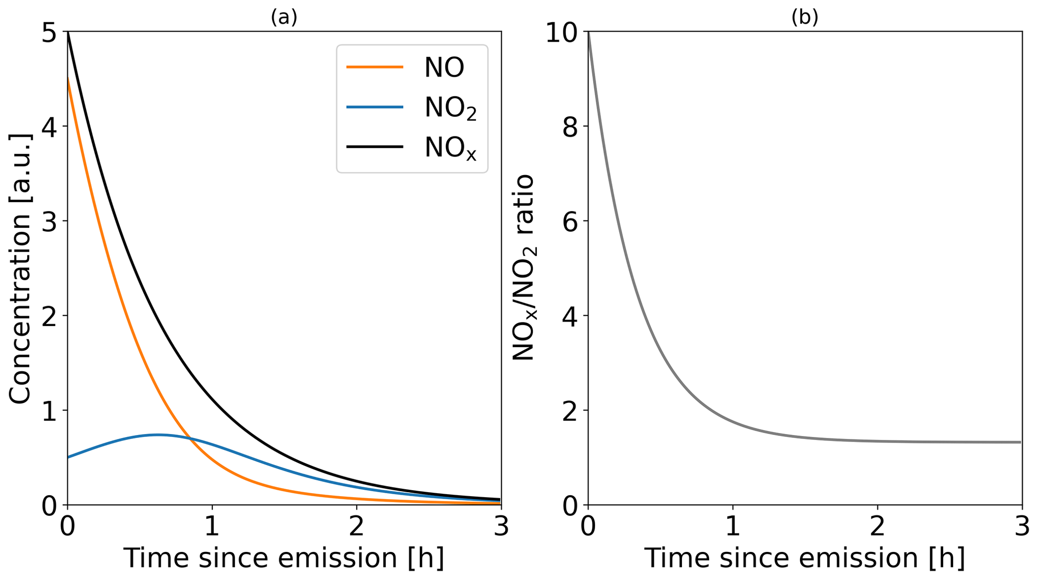
Figure 1(a) Schematic illustration of NO, NO2 and NOx concentrations after the emission of NOx, where 90 % of NOx is emitted as NO. (b) Resulting ratio.
Since the NOx:NO2 ratio inside plumes cannot be assumed to be constant, the aim of this study is to develop a more realistic model for a NO2-to-NOx conversion factor that accounts for the spatiotemporal variations in NOx chemistry in plumes. The model is applied in combination with the cross-sectional flux (CSF) method, which were both implemented in the Python package for “data-driven emission quantification” (see Sect. 2.1.1) (ddeq; Kuhlmann et al., 2024). To develop a more realistic conversion of NO2 to NOx that varies with time since emission and hence with the distance of the cross-section from the source, we use MicroHH simulations that were conducted within the CoCO2 project. Simulations were performed for the power plants in Bełchatów (PL), Jänschwalde (DE), and Matimba and Medupi (ZA) (hereafter referred to as Matimba), as well as a metallurgical plant in Lipetsk (RU). The derived parameterisation is then applied to TROPOMI observations of these four sources over a 2-year period.
2.1 Development of a NO2-to-NOx conversion model using MicroHH simulations
2.1.1 Estimating emissions with the cross-sectional flux method
The CSF method is a common mass-balance approach, which can be used to estimate emissions of point sources. An implementation of the approach is available in the open-source Python library for data-driven emission quantification (ddeq; Kuhlmann et al., 2024). Since the CSF method divides a plume into several cross-sections perpendicular to the plume direction and establishes a plume-following coordinate system with along-plume and across-plume coordinates, it is ideal for studying the progress of the NOx chemistry inside of the plume.

Figure 2Example of the cross-sectional flux method. (a) Satellite image of a NO2 plume divided into sub-polygons. (b) Integrated trace gas concentration for six sub-polygons. For downstream polygons, Eq. (2) is used. For the upstream polygon, the gas columns are summed up. (c) Estimated trace gas fluxes as mass NO2 along the plume and the corresponding fitted function to estimate the emissions.
Figure 2 shows the application of the CSF method for a TROPOMI NO2 image containing the plume from the Matimba and Medupi power plants in South Africa. Note that the power plants are only 6 km apart so that their plumes appear as a single plume in the TROPOMI image. In a first step, a plume detection algorithm is used to determine the location of the plume (Kuhlmann et al., 2019). A centre line is drawn along the ridge of the plume, which is used to compute along- and across-plume coordinates (denoted by x and y, respectively) and to outline the plume area (yellow polygon in Fig. 2a). The polygon is subdivided into sub-polygons of 12 km length (Kuhlmann et al., 2020). For each sub-polygon, the mass of the trace gas enhancement over the background ΔΩ (g m−2) is integrated over the width of the plume, which yields line densities q (g m−1) at distance x:
The plume width is defined as twice the maximum distance of a detected plume pixel from the centre of the curve. As an alternative, the line density q can be computed by fitting a Gaussian curve to the enhancements inside the polygon, perpendicular to the direction of the plume:
with g being the fitted column using the standard width σ and centre position μ to the observations (Kuhlmann et al., 2021). Figure 2b shows the computation of the line densities for six examples at different distances from the plume. The line densities computed from NO2 observations at different distances from the source need to be converted to NOx line densities using a NO2-to-NOx conversion model f that depends on the time since emission t:
The time since emission t is computed from an effective wind speed ueff at the source and the arc length of the centre line (see Sect. 4.3). Details of the estimation of the function f(t) are presented in Sect. 2.1.3.
Finally, the line densities are converted to fluxes F by multiplying them by ueff. Finally, the emission Q is estimated by fitting a negative exponential function to the fluxes F(t), with the additional fit parameter τ representing the NOx lifetime:
Figure 2c shows how NOx and NO2 fluxes evolve with distance from the source. Note that the decrease in the flux is caused by the NOx lifetime τ, while the NO2-to-NOx conversion model f is the ratio of the two lines.
2.1.2 Synthetic satellite observations
We use high-resolution atmospheric transport simulations with chemistry to simulate the NOx and NO2 concentrations inside plumes and to gain a better understanding of the NOx:NO2 ratios in plumes. For this study, we used simulations from the MicroHH large-eddy simulation (LES) (van Heerwaarden et al., 2017), which has recently been extended with a chemistry module (Krol et al., 2024).
The simulations used are part of the library of plumes generated in the CoCO2 project, where different models were used to simulate the plumes of point sources (Krol and van Stratum, 2021; Koene and Brunner, 2022). For the library, MicroHH was run on a 128 km × 128 km × 4 km domain in the latitude, longitude and altitude directions, respectively, for Matimba and a 51.2 km × 51.2 km × 4 km domain for Bełchatów, Jänschwalde and Lipetsk. The spatial resolution was set to 100 m × 100 m × 25 m for the Matimba case and 50 m × 50 m × 25 m for the others. Each case was simulated for 48 h, starting at 00:00 UTC, and the output was saved hourly. The simulation periods were selected based on the availability of measurements from aircraft campaigns and cloud-free TROPOMI images.
Table 1Details of the four MicroHH simulations used in this study. Additional details can be found in Krol et al. (2024).
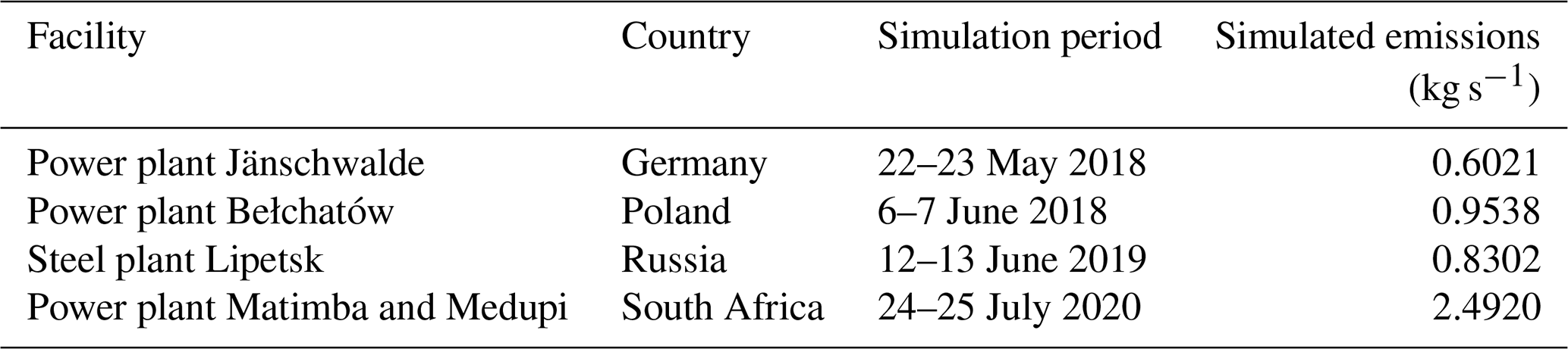
MicroHH simulates reactive trace gases and CO2 as well as meteorological variables such as temperature, pressure and wind speed. The model includes a simplified version of the chemistry scheme implemented in the Integrated Forecasting System (IFS) model of the European Centre for Medium-Range Weather Forecasts (Huijnen et al., 2016), simulating the species O3, NO, NO2, NO3, N2O5, HNO3, CO, CO2, CH4 (fixed), H2 (fixed), HO2, OH, H2O2, CH2O, RO2 and ROOH, as well as C3H6 as a representative of VOCs. The chemistry was tuned to match the NOx and HOx chemistry of IFS and to realistically represent the photostationary state between NO, NO2 and O3. The model was initialised and driven with hourly meteorological data from the ERA5 reanalysis. For the background concentrations of trace gases, reanalysis data from the Copernicus Atmosphere Monitoring Service (CAMS) were used (Krol et al., 2024; van Stratum et al., 2023). To simulate the plumes, typical quantities of NOx emissions from bottom-up-reported values of previous years were released at the respective locations of the power plants and industrial facilities (see Table 1). The NOx emissions were split into 95 % NO and 5 % NO2 by mass (Krol and van Stratum, 2021).
The model output consisted of 3D data of the reactive trace gases as well as meteorological variables such as temperature, pressure and wind speed. The output was post-processed into 2D datasets resembling synthetic satellite observations but without including any measurement noise. The resolution was degraded to the expected resolution of the CO2M satellites of 2 km × 2 km. For the wind speeds, a 2D weighted average of the 3D wind fields was calculated based on the vertical emission profile. The temporal evolution of wind speeds, background concentrations and photolysis rates is displayed in Figs. S1, S2 and S4 in the Supplement. These wind speeds are used to estimate the simulated emissions. The specific model settings and boundary conditions used for the MicroHH model runs are described in Krol and van Stratum (2021) and Krol et al. (2024), while the post-processing is documented in Koene and Brunner (2023).
2.1.3 Conversion of NO2 to NOx line densities in MicroHH
To derive a more realistic conversion model of NO2 to NOx line densities f(t), the vertically integrated MicroHH simulations were analysed for the Bełchatów, Jänschwalde, Lipetsk and Matimba sources by applying the CSF method as outlined above.
We analysed the time steps from 08:00 to 14:00 UTC for both simulated days instead of only the ones at the TROPOMI overpass time to derive more robust NO2-to-NOx conversion factors that better represent varying atmospheric and site conditions. For each polygon of the detected plumes, the line densities of NO and NO2 were calculated. The along-plume distance of each plume was divided by the profile-weighted wind speed at the source to convert them to a time since emission. Such a conversion allows us to account for the effects of varying wind speeds on the concentration of trace gases. For each source, we fitted a negative exponential function to the median NOx:NO2 ratio, using the standard deviations of the analysed time steps as uncertainties.
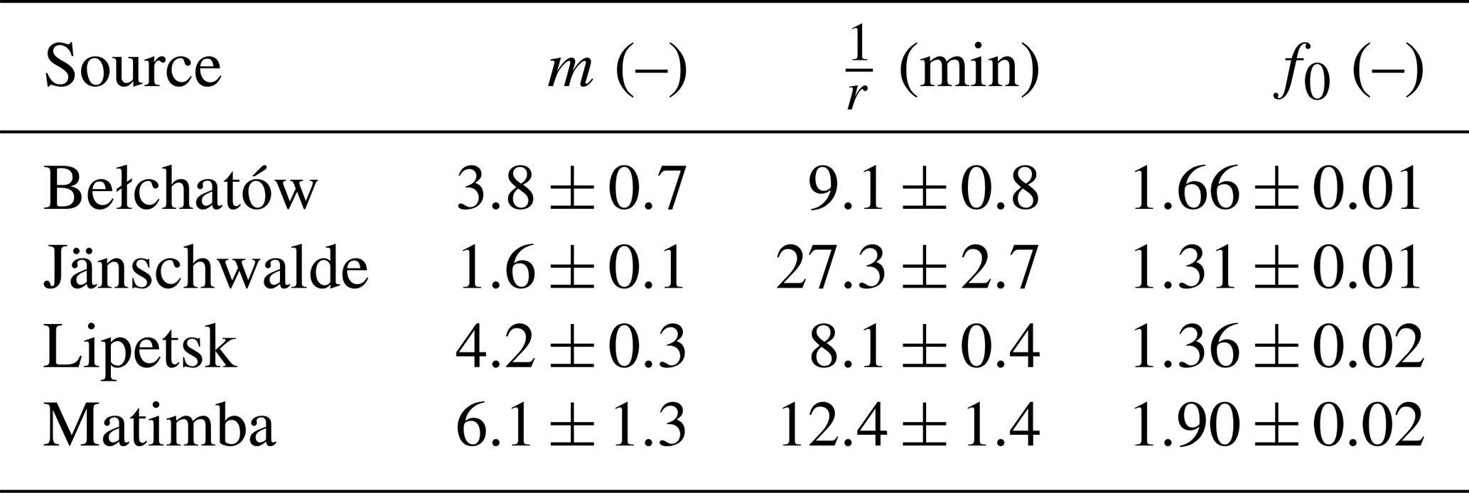
The fitting parameter m represents a scaling factor, r the rate at which the NOx:NO2 ratio decreases and f0 the offset to which the ratio will converge to with time. A negative exponential function was chosen for the conversion of NO2 to NOx to account for the initial increase in NO2 due to the oxidation of NO. The resulting conversion factor f(t) can be multiplied by the corresponding line densities to obtain . The uncertainty σf of f is calculated from the fitted uncertainties in the three parameters by propagation of uncertainty:
and used to update the uncertainty σl of the NOx line densities q:
The method of converting NO2 to NOx presented in this paper relies on the assumption of steady-state conditions and an exponential decay of the conversion factor (Eq. 5). Therefore, it is important to check if NOx emission estimates derived from the time-dependent algorithm are consistent with the emitted quantities. For this purpose, we estimated the NOx emissions of the same daytime time steps of MicroHH three times: once using the modelled NOx fields, once using the NO2 fields and applying the constant NO2-to-NOx conversion factor of 1.32 (referred to as the algorithm with a constant factor), and once using the negative exponential function fitted above as conversion factors (referred to as the time-dependent algorithm).
2.2 Application to TROPOMI NO2 satellite observations
2.2.1 TROPOMI satellite observations
We applied the method of converting NO2 to NOx line densities developed in the current study to the latest processing version (v2.4.0) of the tropospheric NO2 observations from TROPOMI for the years 2020 and 2021 (Copernicus Sentinel-5P, 2021). In accordance with van Geffen et al. (2019), only data with quality assurance values higher than 0.75 were utilised. In addition, we downloaded the auxiliary data comprising 3D NO2 fields from the 3D chemistry-transport model TM5-MP to recompute the air mass factors (AMFs) (see Sect. 2.2.2) (Eskes and van Geffen, 2021). To determine the NO2 line densities, we fit a Gaussian curve (Eq. 2) to the observed NO2 vertical column densities (VCDs) using a weighted least squares (WLS) method. Since the errors in NO2 VCDs depend on the retrieved VCDs, computing the weights from the reported errors would give lower weight to higher VCDs and, as a result, would tend to underestimate the line density. To avoid this, we set the precision of the retrieved tropospheric NO2 VCDs to 7.6 × 10⁻⁷ kg m−2, which corresponds to 1 × 10⁻¹⁵ . This is an average uncertainty over polluted regions and corresponds to approximately 20 % of the measured NO2 VCDs (van Geffen et al., 2019).
Emissions were estimated by applying the constant and time-dependent algorithms to the AMF-corrected images. For each source, the respective fitting parameters m, r and f0 from the MicroHH simulations were used to convert NO2 into NOx. Estimates were then aggregated by month, and annual emissions were estimated as the median of the monthly statistics. This was done to avoid a potential bias due to an unbalanced number of data points per month. To estimate the uncertainty in the annual emissions, a seasonal cycle was fitted to all emission estimates using a cubic Hermite spline with periodic boundary conditions (Kuhlmann et al., 2021). The corresponding uncertainty σe accounts for the uncertainties in the single-overpass estimates through error propagation. To further account for uncertainties in the diurnal (σd) and seasonal (σs) cycles, the total uncertainty σtot was calculated as follows:
Here, both σd and σs were set to 30 % according to Hill and Nassar (2019). As the estimated NOx emissions with the time-dependent algorithm depend on the NO2-to-NOx conversion factor, a sensitivity analysis was performed by applying the NO2-to-NOx conversion factors calculated for Jänschwalde and Matimba to all four sources.
2.2.2 Air mass factor correction
For the retrieval of NO2 VCDs, a priori NO2 profiles from a 3D chemistry transport simulation called TM5-MP are used. Due to its coarse resolution of 1° × 1°, the model cannot resolve individual plumes but rather represents them as smeared-out NO2 enhancements. Consequently, the TM5-MP pixels have neither the correct concentration profile of the plume nor the correct background concentration. This tends to lead to an overestimation of AMFs and consequently an underestimation of VCDs within the observed plumes and, vice versa, outside of the plumes. Such a bias over polluted regions is known from previous studies (Griffin et al., 2019; Verhoelst et al., 2021; Douros et al., 2023). To address these biases we constructed a more realistic NO2 profile that is representative of the observed plumes. To this end, we interpolated the auxiliary data from the TM5-MP model and the ERA5 planetary boundary layer (PBL) height data to the higher-resolution TROPOMI pixels. We set the NO2 mole fraction within the PBL to 5 × 10⁻⁹ mol mol−1 for all detected plume pixels of the images for the years 2020 and 2021. This is an average NO2 concentration within the PBL of detected plumes based on the four MicroHH simulations, independent of the along-plume distance. However, we acknowledge that the profile concentration should ideally decrease along the plume. With the new NO2 profiles xnew, we recalculated the AMFs according to Eskes et al. (2022):
Finally, we updated the VCDs inside the detected plumes for all images using the recalculated AMFnew:
We only recalculated the AMFs and VCDs of detected plume pixels because no other anthropogenic sources other than the power plants and steel plant under consideration were simulated by MicroHH. Thus, the NOx concentrations were too low to obtain representative background concentrations.
2.2.3 ERA5 wind data
The CSF method requires wind data to convert trace gas line densities into fluxes. For this purpose, we weighted the 3D wind fields of the ERA5 reanalysis (Hersbach et al., 2018) with a profile representing the expected vertical distribution of emissions for power plants in Brunner et al. (2019) and integrated them vertically to obtain 2D wind fields. As in Kuhlmann et al. (2021), we assumed a fixed wind speed uncertainty in metres per second (m s−1) for the error propagation in the emission estimation.
2.2.4 Comparison with bottom-up-reported NOx emissions at high temporal resolution
Since the year 2000, member states of the European Union have been required to report the emissions of air and water pollutants from large point sources (European Parliament and the Council of the European Union, 2006). These data were made publicly available in 2006 through the European Pollutant Release and Transfer Register (E-PRTR). The database contains the annual emissions of pollutants from nine major sectors, such as energy production or metal processing, and is available on the European Industrial Emissions Portal (https://industry.eea.europa.eu/, last access: 26 June 2024). We use the bottom-up-reported emissions to assess the accuracy of our emission estimates. We obtained data as annual NOx emissions from the Jänschwalde power plant for the years 2020 to 2021. For the Bełchatów power plant, the data are only available up to 2017. Therefore, we used the CO2 and NOx emissions for 2017 to extrapolate the expected emissions for the years 2020 to 2021 according to Nassar et al. (2022). For the metallurgical plant in Lipetsk, no accurate data on emissions were available since there are no bottom-up-reported emissions for this specific site in the annual report of the operating company NLMK. Moreover, from the reports it is not clear if emissions from the captive power plants at the Lipetsk site are included in the reported emissions. For the Matimba and Medupi power plants, monthly emissions are provided by the operating company Eskom.
For all three power plants, we interpolated the annual and monthly bottom-up-reported CO2 and NOx emissions to hourly and daily temporal resolutions by weighting them with the power plant's energy output according to Nassar et al. (2022). For the European power plants, we used the hourly electricity generation from the transparency platform of the European Network of Transmission System Operators for Electricity (ENTSO-E) (https://transparency.entsoe.eu/, last access: 26 June 2024). For the Matimba and Medupi power plants, we used the daily electricity production provided by the operating company Eskom.
3.1 NOx to NO2 ratios in plumes
An example of the NO2 and NOx vertical column fields simulated with MicroHH for the Matimba case and the corresponding NOx:NO2 ratios is depicted in Fig. 3. The spatiotemporal patterns in the NOx:NO2 ratios of all simulations are displayed in Fig. A1.
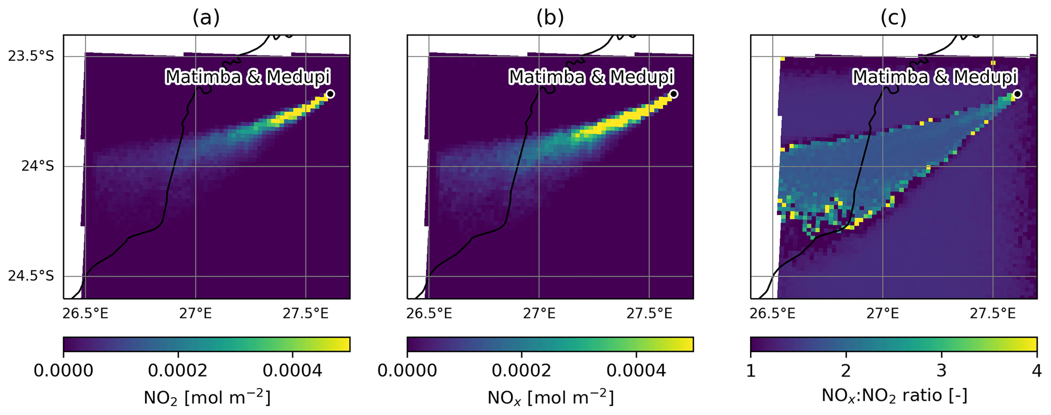
Figure 3Simulated NO2 (a) and NOx (b) fields as well as the resulting NOx:NO2 ratios (c) from time step 32 (08:00 UTC) of the MicroHH simulation of Matimba.
The evolution of NOx:NO2 ratios in the MicroHH model as a function of time since emission is summarised in Fig. 4 for all four cases (Bełchatów, Jänschwalde, Lipetsk and Matimba). The figure contains results from all hourly time steps between 08:00 and 14:00 UTC from both simulated days.

Figure 4Mean NOx:NO2 ratios of the 08:00–14:00 UTC MicroHH time steps as a function of time since emission. (a) Median and standard deviation. (b) Fitted negative exponential function and corresponding standard deviation. The time axis is converted to a space axis using the median wind speed in all analysed plumes.
Figure 4a shows the median and standard deviation of the ratios, while Fig. 4b depicts the corresponding fitted negative exponential functions and the fitted standard deviations. The figure confirms our expectation that the NOx:NO2 ratios are the largest close to the source and decrease with increasing distance downwind. The ratios are generally much larger than the previously used conversion factor f0 = 1.32 (horizontal black line) and only approach this value at distances larger than 50–100 km and only in some cases. Because most of the NOx is emitted as NO, NO concentrations close to the source are very high, which leads to complete titration of O3 present in background air and therefore limits the production of NO2 through the oxidation of NO by O3. With increasing dilution and mixing of the plume with background air downwind of the source, the concentration of NO decreases, while the concentration of O3 increases. This accelerates the oxidation of NO and gradually shifts the photostationary equilibrium ratio of NO:NO2 towards NO2 and reduces the NOx:NO2 ratio accordingly (Seinfeld and Pandis, 2016). Compared to the other three simulations, the NOx:NO2 ratio of the Matimba simulation is higher both at the source and further downwind. The main reason for this behaviour is the amount of NOx emitted: the more NOx that is emitted, the longer it takes for the plume to mix with sufficient O3 from the surrounding air masses to reach the background photostationary state for NOx (Krol et al., 2024). Another reason for the different NOx:NO2 ratios is the meteorological conditions which determine how fast the plumes are mixed with surrounding air masses. Furthermore, the background concentrations of O3 and VOCs that are different for all simulations have a strong influence on the NOx:NO2 ratios and partly explain the higher values of f0 for Bełchatów and Matimba (see Figs. S2–S4) (Seinfeld and Pandis, 2016). In all four simulations, the ratios level off half an hour after the emission or 50 km along the plume, assuming a median wind speed of the analysed time steps of about 5.7 m s−1. Furthermore, Fig. 4 illustrates that the standard deviation close to the source is the largest for Bełchatów, which leads to a higher uncertainty in the fitted function. The corresponding fitting parameters of the NOx:NO2 ratios and their uncertainties are listed in Table 2.
Table 2Fitting parameters of the negative exponential function in Eq. (5) to the mean NOx:NO2 ratios of the four MicroHH simulations for the steps from 08:00 to 14:00 UTC.
To convert NO2 line densities into NOx line densities, they are multiplied by f(t) following Eq. (5). The results for the Matimba plume are shown in Fig. 5. As a result of the multiplication, the NOx line densities peak at the source and approximately follow an exponential decay similar to the schematic in Fig. 1. In contrast, the NO2 line densities peak between 20 and 30 km.

Figure 5Example of estimating NOx emissions from the Matimba MicroHH simulation using the time-dependent conversion of NO2 to NOx for the cross-sectional flux method implemented in ddeq.
Applying the NO2-to-NOx conversion factors to the MicroHH data as a validation in Fig. 6 shows that the estimated NOx emissions with the time-dependent algorithm are in good agreement with the estimates from the modelled NOx fields. However, the spread of the estimates is larger when converting NO2 to NOx, which is due to the assumption that the conversion can be modelled by a negative exponential function. Furthermore, emissions estimated from the modelled NOx fields should align with the prescribed emissions. However, the emissions are overestimated for Bełchatów and Jänschwalde and underestimated for Matimba, which is due to uncertainties in the CSF method (see Sect. 4).
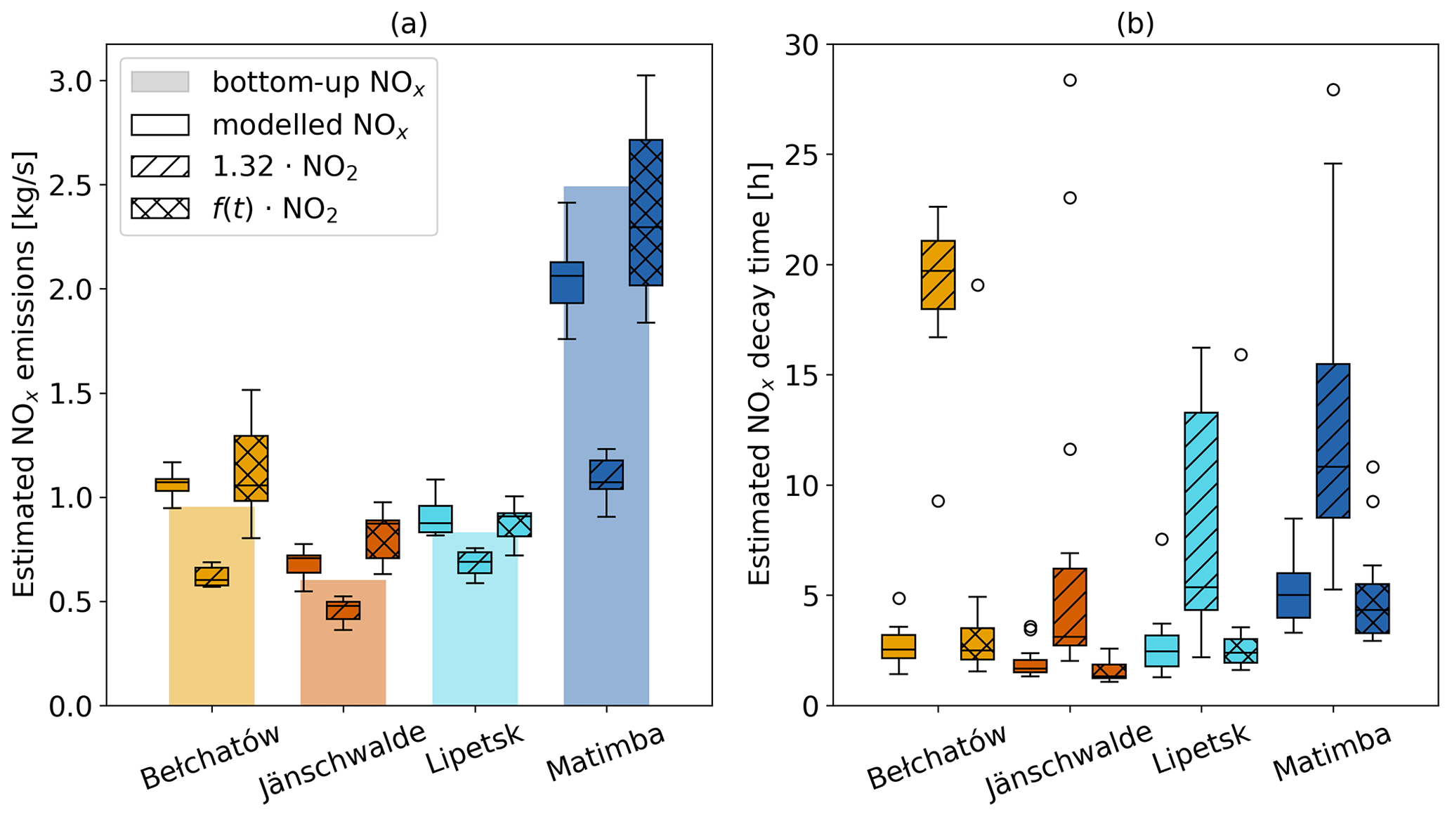
Figure 6(a) Comparison of estimated NOx emissions against the prescribed (bottom-up) emissions and (b) estimated NOx decay times using the constant and time-dependent algorithms as well as the modelled NOx fields. Only the daytime time steps of the MicroHH simulations were utilised. The boxes in the histograms represent the interquartile range (IQR; 25th to 75th percentiles), whiskers the range between Q1 − 1.5 ⋅ IQR and Q3 + 1.5 ⋅ IQR, and circles all data points that fall outside of this range.
Similar to the emission estimates, the estimated NOx decay times using the time-dependent algorithm are more consistent with those from the modelled NOx fields, whereas the estimates using the algorithm with a constant factor are more than twice as high. This overestimation with the algorithm with a constant factor is due to the fact that NO2 decreases less rapidly than NOx due to the gradual shift in the NO:NO2 photostationary equilibrium ratio towards NO2 as mentioned earlier.
The improved agreement between the estimates from modelled NOx fields and the time-dependent algorithm shows that this model of converting NO2 to NOx accounts for the NOx chemistry in the plumes simulated by MicroHH quite well. The larger discrepancies for Bełchatów and Jänschwalde compared to the other cases are probably due to the higher relative uncertainties in the fitted NO2:NOx ratios as seen in Fig. 4b. Nevertheless, the estimated emissions and lifetimes are a significant improvement over the approach of converting NO2 to NOx using a constant factor of 1.32.
3.2 Application of the conversion of NO2 to NOx to TROPOMI observations
For the years 2020 and 2021, a total of 737 TROPOMI images were available for Bełchatów, 807 for Jänschwalde, 862 for Lipetsk and 454 for Matimba. However, for the first three sources, only about 7 % of the images were sufficiently cloud-free. For Bełchatów and Jänschwalde, the plume detection only worked for half of these cloud-free images due to the proximity to other coal-fired powerplants. As a result, the plumes often mixed, rendering the estimation of emissions impossible. For Matimba, almost half of the total available images were cloud-free, with plume detection working on more than 80 % of these images due to the remote location. An example image of the emission estimation for TROPOMI can be seen in Fig. 2.
The AMFs computed for the four cases result in a mean increase in the VCDs inside the plume by a factor of 1.11–1.35 (see Fig. A2). The estimated NOx emissions from the AMF-corrected TROPOMI data for the years 2020 and 2021 are presented in Fig. 7 and listed in Table 3. While the emissions estimated with the algorithm with a constant factor only amount to 48 %–69 % of the bottom-up-reported emissions, the emissions derived with the time-dependent algorithm are more in line and reach about 88 %–109 %. For all four sources, these estimates are within 1 standard deviation of the bottom-up-reported emissions.
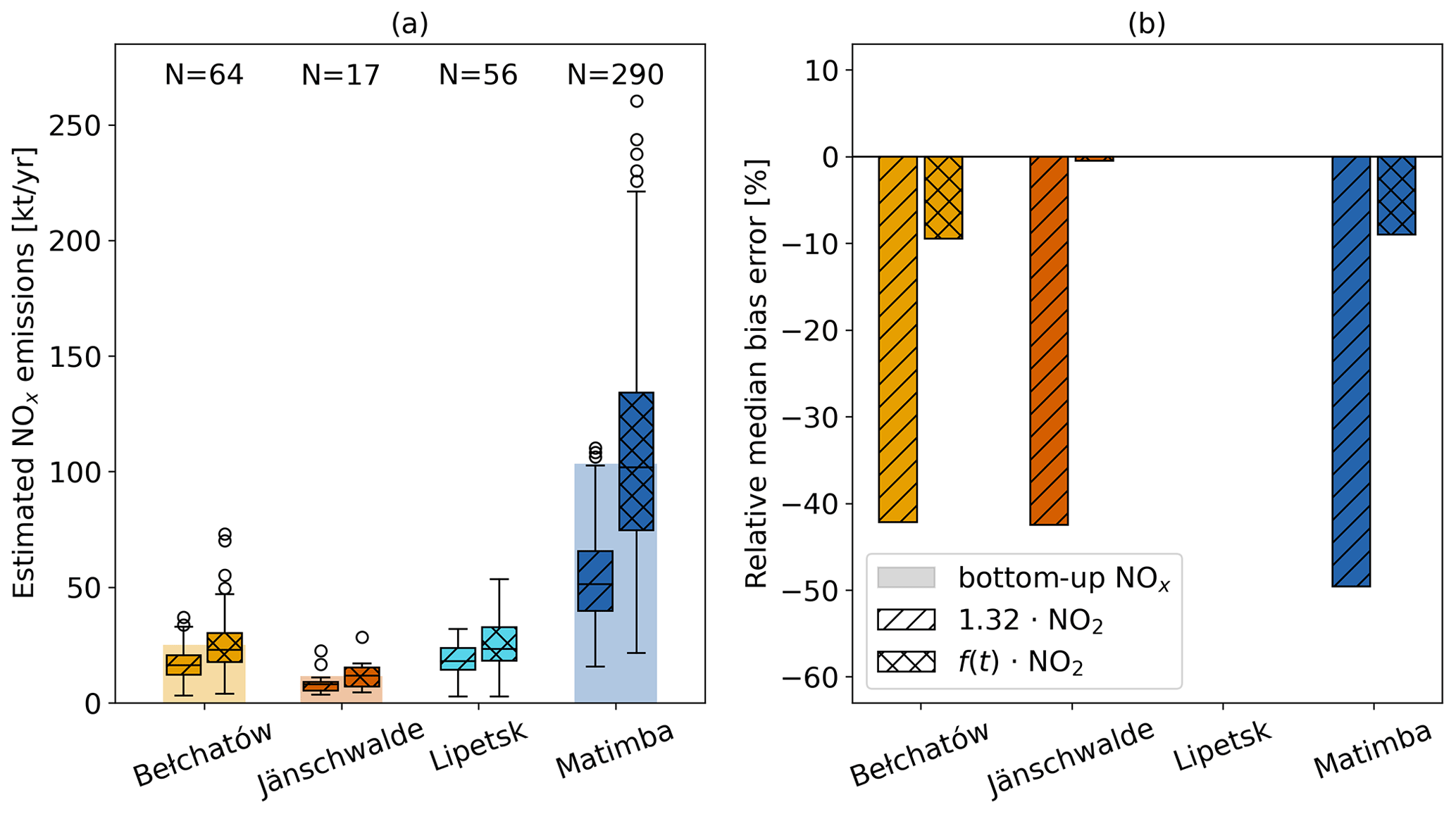
Figure 7(a) Estimated NOx emissions and (b) their median bias errors relative to the bottom-up-reported emissions for Bełchatów, Jänschwalde, Lipetsk and Matimba for TROPOMI data of the years 2020 and 2021.
Table 3Median and standard deviation of estimated NOx emissions in kt NO2 a−1 for the years 2020 and 2021 for Bełchatów, Jänschwalde, Lipetsk and Matimba derived from TROPOMI images.

Figure 7 also shows that the range of estimated emissions is the largest for Matimba with a large number of outliers. The most likely explanation is that the plumes are the longest for this source, meaning that parts of the plume are several hours old and have likely been subject to different chemistry and wind speeds (see Fig. A6). This leads to strong violations of the assumed steady-state conditions along the plume and results in outliers in the NOx fluxes along the plume. The relative mean bias error of a given method is in a similar range for all four sources. While the bias is around −50 % relative to the bottom-up-reported emissions with the algorithm with a constant factor, it is reduced to between only −9.5 % and −0.5 % with the time-dependent algorithm.
The uncertainties in the single-overpass and annual estimates are listed in Table 4. The first column shows the median uncertainty in all single-overpass estimates. The second column represents the standard deviation of the difference between estimated and bottom-up emissions. The uncertainties in the first column would agree with those in the second if the bottom-up-reported emissions corresponded to the true emissions and all uncertainties were included in the emission estimation. However, the larger magnitude of the values in the second column indicates uncertainties in bottom-up-reported emissions (e.g. due to the temporal interpolation) and the presence of other uncertainties in the emission estimation which were not considered. These include the simplified representation of instrument noise, wind speed and AMF correction. On top of these random errors, there are uncertainties due to systematic errors, such as the estimation of background concentrations, the application of the NO2-to-NOx conversion factors to annual data and methodological uncertainties, which are not represented in the estimated uncertainties.
Table 4Uncertainties in NOx emission estimates for single-overpass and annual estimates for Bełchatów, Jänschwalde, Lipetsk and Matimba.

The third column in Table 4 shows the uncertainties in annual emissions according to error propagation, while the fourth column additionally accounts for uncertainties in diurnal and seasonal cycles.
A simple sensitivity analysis in which the NO2-to-NOx conversion factors of Jänschwalde and Matimba were applied to all four sources resulted in emission estimates ranging from 10 % lower to 50 % higher than the estimates shown in Fig. 7. This illustrates that the parameterisation of the conversion of NO2 to NOx depends on the specific situation, such as meteorological conditions, background concentrations and emission strength, and not representing this situation appropriately adds a significant uncertainty to the emission estimates. To get a better understanding of these uncertainties, it would be necessary to run more high-resolution chemistry transport simulations covering a wider range of conditions and to account for these conditions in an extended parameterisation. These simulations could be used to generate a look-up table for the NO2-to-NOx conversion parameters for different conditions. Despite its simplicity, the first-order parameterisation proposed here, which builds on a small set of high-resolution MicroHH simulations for each source, already leads to a substantial reduction in the bias.
4.1 Strengths and weaknesses of the time-dependent conversion of NO2 to NOx
The analysis of NOx:NO2 ratios in modelled plumes demonstrated the importance of chemical processes, leading to a general decrease in this ratio with distance from the source, but it also revealed considerable variability from case to case, which is likely the result of different amounts of emitted quantities, background concentrations, temperatures, and wind and turbulent mixing conditions. The aim of the time-dependent algorithm developed in this study is to reproduce the NO2-to-NOx conversion of line densities along the plume (Fig. 1). If the true chemistry is well approximated, this should lead to good agreement with the prescribed emissions. The remaining discrepancy is therefore due to deviations from our simplified assumptions (e.g. the assumption of an exponential decay of the ratios along the plume) and due to uncertainties in the CSF method. One important source of uncertainty in the CSF method is the wind speed used to convert line densities to fluxes, which is discussed in Sect. 4.3. The errors in the time-dependent algorithm are more in line with those of the modelled NOx fields but are slightly larger because the implemented conversion of NO2 to NOx does not take into account the specific meteorological and background conditions of each time step but is based on the median conditions. Thus, the bias is likely to increase when the NO2-to-NOx conversion factors derived in this study are applied to annual data, as the chemical and meteorological conditions vary considerably during a year. Nevertheless, we argue that applying the four fitted NO2-to-NOx conversion functions to annual TROPOMI images yields suitable emission estimates because most of the images that can be used for plume detection were acquired between April and October (see Fig. A3). Images taken during the rest of the year often cannot be used for NOx estimation due to high cloud cover. Consequently, the prevailing conditions for most of the emission estimates are comparable to the conditions in the MicroHH model simulations, which represent days in May to July. This is supported by Fig. A7, which shows that the simulated wind speeds of the time steps used for the analysis at the source locations are within the interquartile range of ERA5 wind speeds for the same locations for the years 2020 and 2021. As the newly implemented conversion function for NO2 to NOx showed a significant improvement in the estimation of NOx emissions and lifetimes from MicroHH simulations, we consider it suitable for the application to TROPOMI images.
4.2 Quantification of NOx emissions using TROPOMI observations
The application of the time-dependent conversion of NO2 to NOx to the TROPOMI data in Fig. 7 has shown that the NOx emission estimates obtained with the time-dependent algorithm are much closer to the bottom-up-reported emissions than the estimates from the algorithm with a constant NO2-to-NOx conversion factor of 1.32. The relative median bias is reduced from between −50 % and −42 % to only between −9.5 % and −0.5 %. However, the significant variance in estimated emissions for Matimba indicates the necessity for further refinement of the approach. One improvement would be to investigate very long plumes that have been subject to different meteorological conditions than those under which the NO2-to-NOx conversion factors were derived.
As the number of successful emission estimates per year has a strong influence on the uncertainties in the annual emission estimates, maximising the number of suitable satellite images is crucial. Nevertheless, only a fraction of the TROPOMI images could be used for Bełchatów, Jänschwalde and Lipetsk due to cloud cover. Between October and February in particular, emissions could only be estimated for a few days (see Fig. A3). The strong seasonal bias in the number of successful estimates may lead to an underestimation of annual emissions as emissions in winter are expected to be larger due to the higher demand for electricity and heating. This gap cannot be filled by the upcoming polar-orbiting Sentinel-5 satellite either but could be alleviated by existing and upcoming geostationary satellites, such as GEMS, TEMPO and Sentinel-4: the hourly temporal resolution increases the probability of obtaining a usable image on a cloudy day. Multiple images during a day would also allow the diurnal cycle of NOx emissions to be resolved, which currently cannot be captured with only one or two overpasses around noon. However, GEMS, Sentinel-4 and Sentinel-5 have a coarser resolution compared to Sentinel-5P. The complications caused by a coarse spatial resolution can be seen in the example of Jänschwalde: as there are two coal-fired power plants in the vicinity of Jänschwalde (e.g. the Boxberg and Schwarze Pumpe power plants), the plumes often mix, which is why the emissions cannot be estimated reliably using the CSF method. This applies to a lesser extent to Bełchatów. In contrast, fewer sources that could lead to overlapping plumes are located around Lipetsk and Matimba. As shown in Kuhlmann et al. (2021), a satellite with higher spatial resolution, such as CO2M, can help to better differentiate between plumes, mitigating the challenge of overlapping plumes.
The comparison of the uncertainties in the NOx emission estimates in this study with those in Kuhlmann et al. (2021) highlights the importance of the number of successful emission estimates. The uncertainties in the annual emissions of 4 % to 21 % in this study are significantly lower than the uncertainties of 16 % to 73 % and 13 % to 52 % for two and three of the CO2M satellites in Kuhlmann et al. (2021). The reasons are the higher temporal resolution of TROPOMI compared to CO2M and the high source strength of the power plants considered in the current study. The single-overpass estimates due to random error, in contrast, are only marginally lower in this study than the 29 % derived in Kuhlmann et al. (2021). This difference may be attributed to the consideration of additional uncertainties in their study by including a source-strength-dependent factor and an offset.
The systematic biases due to the application of the NO2-to-NOx conversion factors to annual TROPOMI data were investigated in the form of a sensitivity analysis. Applying the NO2-to-NOx conversion factors of Jänschwalde and Matimba to all four sources resulted in emission estimates ranging from 10 % lower to 50 % higher, which illustrates that the parameterisation of the conversion of NO2 to NOx still adds a significant but unknown uncertainty to the emission estimates. This is because it is not possible to determine how well the conditions under which these parameterisations were derived match those of a given TROPOMI image. However, since most of the suitable satellite images are from the season for which the MicroHH simulations were run, we argue that the calculated NO2-to-NOx conversion factors are likely to be in good agreement with the conditions of the TROPOMI images.
Overall, the application of the newly developed NO2-to-NOx conversion factors resulted in more accurate emission estimates compared to the previous constant conversion factor of 1.32. Nevertheless, extrapolating the conversion factors for different meteorological and background conditions remains a challenge.
4.3 Effective wind speeds in plumes
Apart from the NOx chemistry, a realistic representation of the effective wind speed at which the plume is transported is a key issue. This includes the vertical averaging of 3D wind fields and the consideration of time-varying wind fields. To address the first challenge, the 3D wind speeds were weighted with the expected emission profiles. An advantage of this method is that the weighted winds correspond better to the plume when it is not yet well mixed within the PBL, i.e. close to the source or in a stably stratified atmosphere. However, with increasing distance from the source, the trace gases become progressively more well mixed within the PBL. Depending on meteorological conditions, homogeneous mixing can occur within the first few kilometres of the plume (Krol et al., 2024). In such cases, it would be more reasonable to use the mean wind speed within the PBL. Furthermore, Brunner et al. (2019) have shown that plumes typically rise to a height of 250 m in winter but up to 360 m in summer. Winds are strongly influenced by the dynamics of the PBL, which has a distinct diurnal cycle, especially in summer. These results suggest that a fixed emission profile is likely not sufficient to vertically weigh the 3D wind fields. Instead, the effective wind should be calculated dynamically and account for parameters such as stack height, flue gas properties and meteorological conditions (Brunner et al., 2019). Ultimately, further studies are needed to assess the suitability of this method to vertically average the wind speeds under different conditions.
4.4 Impact of air mass factors
The coarse resolution of the a priori NO2 profiles used for the retrieval of NO2 VCDs leads to an underestimation of VCDs within the plume and an overestimation outside. As the NO2 background VCDs are subtracted from the plume enhancements, updating the NO2 profiles both within and outside the plume would further increase NOx emission estimates. This would lead to higher emission estimates and possibly an overestimation, which would be in line with the slight overestimation of NOx emissions when using the time-dependent algorithm in Fig. 6 for the same reasons as discussed in Sect. 3.1.
Ideally, the a priori NO2 profiles of the TM5-MP model should be replaced by profiles from higher-resolution models such as GEM-MACH (Goldberg et al., 2019b) or CAMS regional (Douros et al., 2023). However, updating the AMFs for all pixels was beyond the scope of this study. For this reason, the a priori NO2 profiles of plume pixels were replaced by a constant NO2 mole fraction of 5 × 10⁻⁹ mol mol−1 within the PBL. This resulted in lower AMFs and consequently higher VCDs by a factor of 1.15 to 1.35. Other studies have calculated significantly larger corrections. For example, Beirle et al. (2019) found that the VCD excess needs to be corrected by a factor of 1.35 for South Africa and 1.98 for Germany. The higher values are attributed to the assumption made by Beirle et al. (2019) that the entire plume is confined between 60 and 200 m above ground level, where the height-resolved AMFs are typically smaller than at higher altitudes. In contrast, the correction factors in this study were calculated assuming a homogeneous distribution within the PBL, which is more realistic and in line with the MicroHH simulations. Douros et al. (2023) analysed the impact of replacing the TROPOMI a priori NO2 profiles over Europe with data from the higher-resolution CAMS regional model at a resolution of 0.1° × 0.1°. They found that the NO2 VCDs increased by a factor of 1.05 for less polluted sites and up to 1.3 for more polluted sites, which is in good agreement with the increases in VCDs calculated in this study. We conducted a sensitivity study with the MicroHH profiles of Matimba to assess the impact of varying NO2 profiles inside the plume, showing that the use of the AMF calculated when assuming constant NO2 PBL concentrations to convert slant column densities (SCDs) to VCDs leads to an underestimation of 8.5 % compared to when using the true MicroHH NO2 VCDs (see Fig. S5).
4.5 Bottom-up-reported emissions
In this study, knowledge of bottom-up-reported NOx and CO2 emissions is important for two reasons. Firstly, they are used to evaluate the accuracy of the estimated NOx emissions from satellites. Secondly, reported emissions can be used to convert the estimated NOx emissions into CO2. For both applications it is crucial to have information on the reliability and accuracy of the bottom-up-reported emissions. However, many of the bottom-up-reported CO2 emissions are estimated from fuel consumption, making assumptions about combustion efficiency, fuel purity and other factors difficult, introducing many uncertainties, which are difficult to quantify (IPCC, 2006). It is assumed that bottom-up uncertainties for CO2 are in the range of ± 10 % (Gurney et al., 2016) but significantly higher for NOx (e.g. Zhao et al., 2011). Deviations between estimated and bottom-up-reported emissions are therefore not necessarily due to errors in the estimates but could also originate from inaccuracies in the reported emissions.
In this study, we derived a more realistic model for the conversion of NO2 to NOx in plumes of large-NOx sources. We derived parameters for this model using high-resolution chemistry transport model simulations. The conversion model was then applied to TROPOMI observations from 2020 to 2021.
The results show that annual NOx emissions can be reliably estimated with TROPOMI: the discrepancies between bottom-up and top-down estimates were reduced from between −50 % and −42 % to only between −9.5 % and −0.5 %, with uncertainties ranging from 4 % to 21 %. These more accurate NOx emission estimates are important for air quality monitoring and can be used to convert NOx to CO2 emissions using CO2:NOx emission ratios, allowing for the use of NO2 imaging satellites such as GEMS, TEMPO, Sentinel-4 and Sentinel-5 to estimate CO2 emission with high temporal resolution. Furthermore, geostationary satellites will allow researchers to better resolve the diurnal cycle of emissions and could help to reduce a potential seasonal bias by reducing the number of failed emission estimates caused by cloud cover.
This study also highlights several shortcomings of the current approach. More comprehensive and systematic studies are necessary to determine the dependence of the NO2-to-NOx conversion factor on prevailing conditions such as wind speed, atmospheric stability, solar radiation, temperature and background concentrations of reactive trace gases. An alternative approach for converting NO2 to NOx line densities would be to use machine learning such as neural networks. Once trained with a high-resolution model with chemistry like MicroHH, the network could predict the NO2-to-NOx conversion factors without the need to run a high-resolution chemistry transport model for each plume. However, a large number of simulations covering a wide range of conditions would need to be run for proper training and validation of a machine learning model. Furthermore, as mentioned earlier, more research is necessary to determine how wind speeds should be vertically averaged in plumes and how systematic uncertainties due to AMFs can be best accounted for.
The time-dependent NO2-to-NOx conversion model has been implemented in ddeq and can be adjusted for different sources and conditions. A Jupyter Notebook using Python is available in the Supplement, which provides easy access to the implementations and enables users to estimate NOx emissions from NO2 satellite observations of specific sources using their own set of NO2-to-NOx conversion parameters. These emissions can then be converted to CO2 emissions using CO2:NOx ratios. Therefore, the current study is an important step towards consistent, uniform, high-resolution and near-real-time estimation of NOx and CO2 emissions with the use of satellites, which is crucial for air quality monitoring and greenhouse gas emission monitoring and verification.
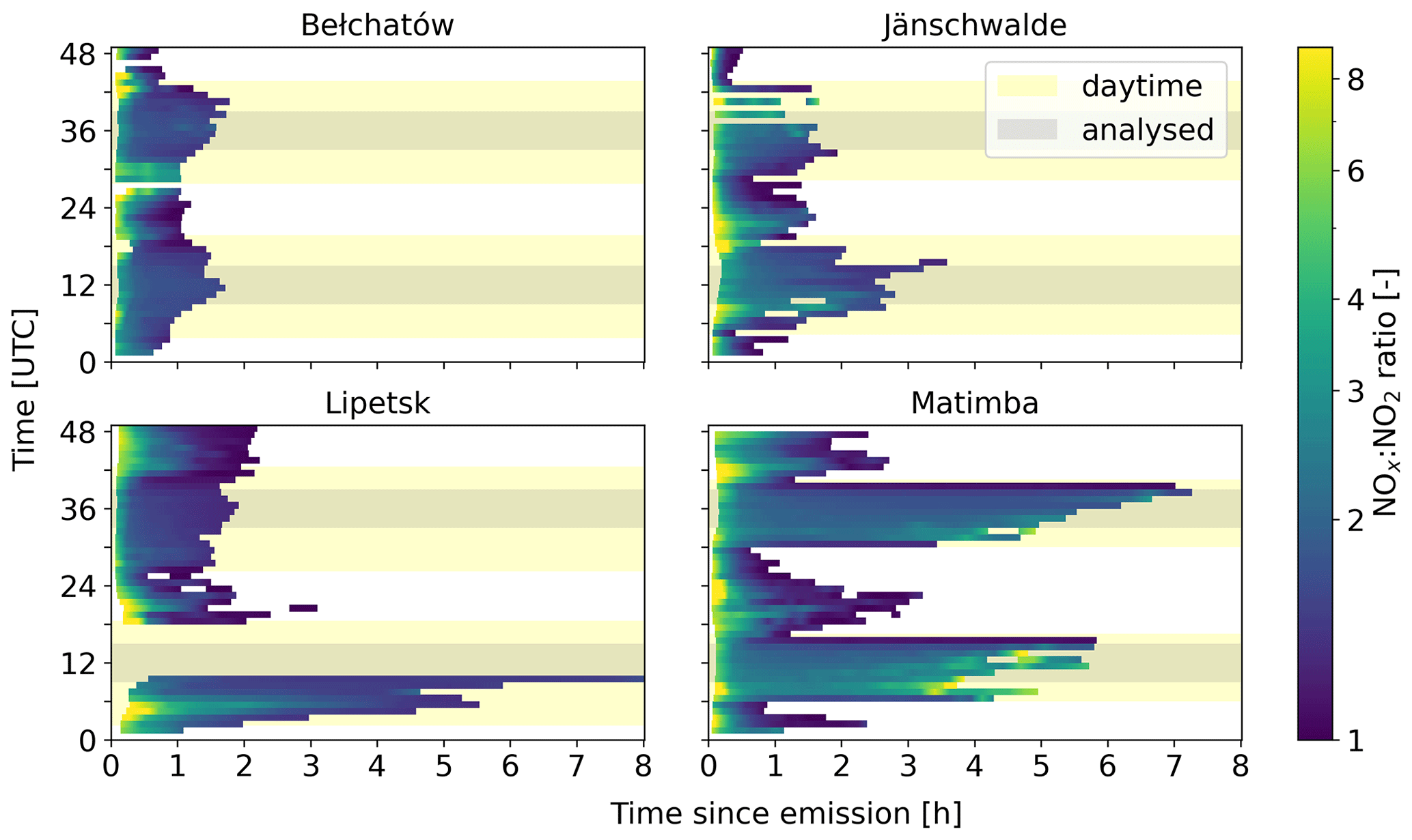
Figure A1NOx:NO2 ratios for 48 individual hourly time steps of the MicroHH simulations of Bełchatów, Jänschwalde, Lipetsk and Matimba as a function of time since emission, highlighting the spatiotemporal patterns in the NOx chemistry. The yellow shading represents daytime, and the grey shading represents the time steps used in the analysis.
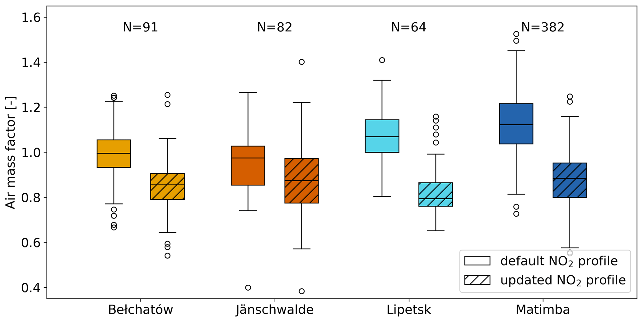
Figure A2Default and updated AMF of TROPOMI images of Bełchatów, Jänschwalde, Lipetsk and Matimba for the years 2020 and 2021. For the updated AMFs, the NO2 mole fraction was set to 5 × 10⁻⁹ mol mol−1 within the PBL of the detected plumes.

Figure A3Number of successful NOx emission estimates per month using TROPOMI for 2020 and 2021.
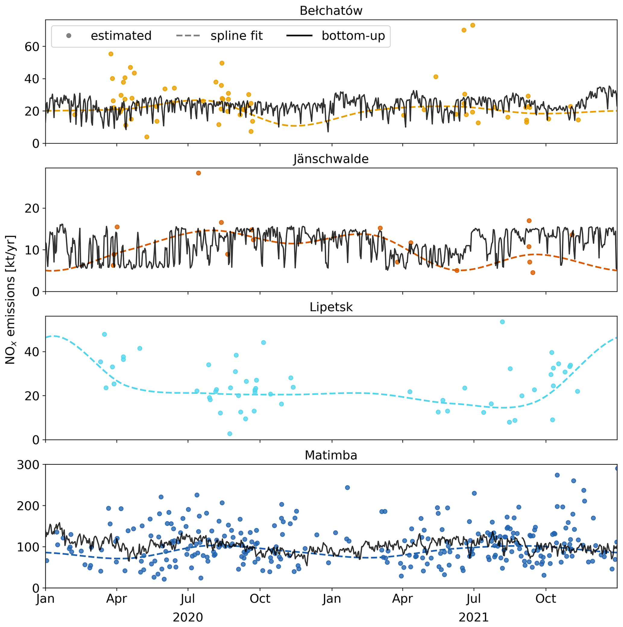
Figure A4Time series of NOx emission estimates using TROPOMI and bottom-up-reported emissions for the years 2020 and 2021. A cubic Hermite spline with periodic boundary conditions was fitted to each time series.

Figure A5(a) TM5-MP and MicroHH NO2 profiles of the Sentinel-5P source pixel for Matimba on 25 July 2020 at 12:00 UTC. (b) Histogram of the default and recalculated AMFs of the TROPOMI pixel containing the Matimba power plant based on MicroHH NO2 profiles.

Figure A6Maximum lengths and ages of detected plumes from TROPOMI observations for the years 2020 and 2021. Ages were calculated by dividing the plume length by the profile-weighted wind speed at the source.

Figure A7Vertically integrated ERA5 wind speeds at TROPOMI overpass time for the years 2020 and 2021 and vertically integrated simulated wind speeds in MicroHH for the time steps from 08:00 to 14:00 UTC on both simulated days. For both variables, the wind speed was sampled at the location of the Bełchatów, Jänschwalde, Lipetsk and Matimba sources.
Data-driven emission quantification version 1.0 used for this study is available on GitLab.com (https://gitlab.com/empa503/remote-sensing/ddeq, Kuhlmann et al., 2024). MicroHH data can be downloaded on Zenodo at https://doi.org/10.5281/zenodo.7448144 (Koene and Brunner, 2022). An example notebook on how to use the conversion of NO2 to NOx covered in this paper can be found in the Supplement. ERA5 data are available at https://doi.org/10.24381/cds.adbb2d47 (Hersbach et al., 2018). TROPOMI data are available at https://doi.org/10.5270/S5P-9bnp8q8 (Copernicus Sentinel-5P, 2021).
The supplement related to this article is available online at: https://doi.org/10.5194/acp-24-7667-2024-supplement.
SM conducted the analysis and wrote the paper with input from all co-authors; EK processed the MicroHH model simulations into pseudo-satellite images; MK provided insight into the MicroHH simulations and NOx chemistry; DB and AD offered constructive feedback on the paper; GK coordinated and supervised the project.
The contact author has declared that none of the authors has any competing interests.
Publisher's note: Copernicus Publications remains neutral with regard to jurisdictional claims made in the text, published maps, institutional affiliations, or any other geographical representation in this paper. While Copernicus Publications makes every effort to include appropriate place names, the final responsibility lies with the authors.
We would like to acknowledge the ICOS Carbon Portal for providing the computational resources needed for the analysis shown in this paper.
This research has been supported by the EU's Horizon Digital, Industry and Space project (CORSO; grant no. 101082194) and the Staatssekretariat für Bildung, Forschung und Innovation (SERI; grant no. 22.00422).
This paper was edited by Michel Van Roozendael and reviewed by two anonymous referees.
Beirle, S., Boersma, K. F., Platt, U., Lawrence, M. G., and Wagner, T.: Megacity Emissions and Lifetimes of Nitrogen Oxides Probed from Space, Science, 333, 1737–1739, https://doi.org/10.1126/science.1207824, 2011. a
Beirle, S., Borger, C., Dörner, S., Li, A., Hu, Z., Liu, F., Wang, Y., and Wagner, T.: Pinpointing nitrogen oxide emissions from space, Science Advances, 5, eaax9800, https://doi.org/10.1126/sciadv.aax9800, 2019. a, b
Beirle, S., Borger, C., Dörner, S., Eskes, H., Kumar, V., de Laat, A., and Wagner, T.: Catalog of NOx emissions from point sources as derived from the divergence of the NO2 flux for TROPOMI, Earth Syst. Sci. Data, 13, 2995–3012, https://doi.org/10.5194/essd-13-2995-2021, 2021. a
Bovensmann, H., Buchwitz, M., Burrows, J. P., Reuter, M., Krings, T., Gerilowski, K., Schneising, O., Heymann, J., Tretner, A., and Erzinger, J.: A remote sensing technique for global monitoring of power plant CO2 emissions from space and related applications, Atmos. Meas. Tech., 3, 781–811, https://doi.org/10.5194/amt-3-781-2010, 2010. a
Brunner, D., Kuhlmann, G., Marshall, J., Clément, V., Fuhrer, O., Broquet, G., Löscher, A., and Meijer, Y.: Accounting for the vertical distribution of emissions in atmospheric CO2 simulations, Atmos. Chem. Phys., 19, 4541–4559, https://doi.org/10.5194/acp-19-4541-2019, 2019. a, b, c
Copernicus Sentinel-5P (processed by ESA): TROPOMI Level 2 Nitrogen Dioxide total column products, Version 02, European Space Agency [data set], https://doi.org/10.5270/S5P-9bnp8q8, 2021. a, b
de Foy, B., Lu, Z., Streets, D. G., Lamsal, L. N., and Duncan, B. N.: Estimates of power plant NOx emissions and lifetimes from OMI NO2 satellite retrievals, Atmos. Environ., 116, 1–11, https://doi.org/10.1016/j.atmosenv.2015.05.056, 2015. a
Douros, J., Eskes, H., van Geffen, J., Boersma, K. F., Compernolle, S., Pinardi, G., Blechschmidt, A.-M., Peuch, V.-H., Colette, A., and Veefkind, P.: Comparing Sentinel-5P TROPOMI NO2 column observations with the CAMS regional air quality ensemble, Geosci. Model Dev., 16, 509–534, https://doi.org/10.5194/gmd-16-509-2023, 2023. a, b, c, d
Eskes, H. and van Geffen, J.: Product user manual for the TM5 NO2, SO2 and HCHO profile auxiliary support product, Tech. rep., KNMI, S5P-KNMI-L2-0035-MA, https://sentinel.esa.int/documents/247904/2474726/PUM-for-the-TM5-NO2-SO2-and-HCHO-profile-auxiliary-support-product.pdf/de18a67f-feca-1424-0195-756c5a3df8df (last access: 26 June 2024), 2021. a
Eskes, H., van Geffen, J., Boersma, F., Eichmann, K.-U., Apituley, A., Pedergnana, M., Sneep, M., Veefkind, J., and Loyola, D.: Sentinel-5 precursor/TROPOMI Level 2 Product User Manual Nitrogendioxide, Tech. rep., KNMI, S5P-KNMI-L2-0021-MA, https://sentinel.esa.int/documents/247904/2474726/Sentinel-5P-Level-2-Product-User-Manual-Nitrogen-Dioxide.pdf(last access: 26 June 2024), 2022. a
European Parliament and the Council of the European Union: REGULATION (EC) No 166/2006: Establishment of a European Pollutant Release and Transfer Register and amending Council Directives 91/689/EEC and 96/61, Official Journal of the European Union, http://data.europa.eu/eli/reg/2006/166/oj (last access: 26 June 2024), 2006. a
Goldberg, D. L., Lu, Z., Oda, T., Lamsal, L. N., Liu, F., Griffin, D., McLinden, C. A., Krotkov, N. A., Duncan, B. N., and Streets, D. G.: Exploiting OMI NO2 satellite observations to infer fossil-fuel CO2 emissions from US megacities, Sci. Total Environ., 695, 133805, https://doi.org/10.1016/j.scitotenv.2019.133805, 2019a. a
Goldberg, D. L., Lu, Z., Streets, D. G., de Foy, B., Griffin, D., McLinden, C. A., Lamsal, L. N., Krotkov, N. A., and Eskes, H.: Enhanced capabilities of TROPOMI NO2: Estimating NOx from north american cities and power plants, Environ. Sci. Technol., 53, 12594–12601, 2019b. a, b, c
Goldberg, D. L., Harkey, M., de Foy, B., Judd, L., Johnson, J., Yarwood, G., and Holloway, T.: Evaluating NOx emissions and their effect on O3 production in Texas using TROPOMI NO2 and HCHO, Atmos. Chem. Phys., 22, 10875–10900, https://doi.org/10.5194/acp-22-10875-2022, 2022. a
Griffin, D., Zhao, X., McLinden, C. A., Boersma, F., Bourassa, A., Dammers, E., Degenstein, D., Eskes, H., Fehr, L., Fioletov, V., Hayden, K., Kharol, S. K., Li, S.-M., Makar, P., Martin, R. V., Mihele, C., Mittermeier, R. L., Krotkov, N., Sneep, M., Lamsal, L. N., ter Linden, M., van Geffen, J., Veefkind, P., and Wolde, M.: High-resolution mapping of nitrogen dioxide with TROPOMI: First results and validation over the Canadian oil sands, Geophys. Res. Lett., 46, 1049–1060, 2019. a
Gurney, K. R., Huang, J., and Coltin, K.: Bias present in US federal agency power plant CO2 emissions data and implications for the US clean power plan, Environ. Res. Lett., 11, 064005, https://doi.org/10.1088/1748-9326/11/6/064005, 2016. a
Hakkarainen, J., Ialongo, I., Oda, T., Szeląg, M. E., O'Dell, C. W., Eldering, A., and Crisp, D.: Building a bridge: characterizing major anthropogenic point sources in the South African Highveld region using OCO-3 carbon dioxide snapshot area maps and Sentinel-5P/TROPOMI nitrogen dioxide columns, Environ. Res. Lett., 18, 035003, https://doi.org/10.1088/1748-9326/acb837, 2023. a
Hakkarainen, J., Kuhlmann, G., Koene, E., Santaren, D., Meier, S., Krol, M. C., van Stratum, B. J., Ialongo, I., Chevallier, F., Tamminen, J., Brunner, D., and Broquet, G.: Analyzing nitrogen dioxide to nitrogen oxide scaling factors for data-driven satellite-based emission estimation methods: A case study of Matimba/Medupi power stations in South Africa, Atmos. Pollut. Res., 15, 102171, https://doi.org/10.1016/j.apr.2024.102171, 2024. a
Hersbach, H., Bell, B., Berrisford, P., Biavati, G., Horányi, A., Muñoz Sabater, J., Nicolas, J., Peubey, C., Radu, R., Rozum, I., Schepers, D., Simmons, A., Soci, C., Dee, D., and Thépaut, J.-N.: ERA5 hourly data on single levels from 1940 to present, Copernicus Climate Change Service (C3S) Climate Data Store (CDS) [data set], https://doi.org/10.24381/cds.adbb2d47, 2018. a, b
Hill, T. and Nassar, R.: Pixel size and revisit rate requirements for monitoring power plant CO2 emissions from space, Remote Sens., 11, 1608, https://doi.org/10.3390/rs11131608, 2019. a
Huijnen, V., Flemming, J., Chabrillat, S., Errera, Q., Christophe, Y., Blechschmidt, A.-M., Richter, A., and Eskes, H.: C-IFS-CB05-BASCOE: stratospheric chemistry in the Integrated Forecasting System of ECMWF, Geosci. Model Dev., 9, 3071–3091, https://doi.org/10.5194/gmd-9-3071-2016, 2016. a
IPCC: 2006 IPCC guidelines for national greenhouse gas inventories, Institute for Global Environmental Strategies, ISBN 4-88788-032-4, 2006. a
Janssens-Maenhout, G., Pinty, B., Dowell, M., Zunker, H., Andersson, E., Balsamo, G., Bézy, J.-L., Brunhes, T., Bösch, H., Bojkov, B., Brunner, D., Buchwitz, M., Crisp, D., Ciais, P., Counet, P., Dee, D., Denier van der Gon, H., Dolman, H., Drinkwater, M., Dubovik, O., Engelen, R., Fehr, T., Fernandez, V., Heimann, M., Holmlund, K., Houweling, S., Husband, R., Juvyns, O., Kentarchos, A., Landgraf, J., Lang, R., Löscher, A., Marshall, J., Meijer, Y., Nakajima, M., Palmer, P., Peylin, P., Rayner, P., Scholze, M., Sierk, B., Tamminen, J., and Veefkind, P.: Towards an operational anthropogenic CO2 emissions monitoring and verification support capacity, B. Am. Meteorol. Soc., 101, 1439–1451, https://doi.org/10.1175/BAMS-D-19-0017.1, 2020. a
Koene, E. and Brunner, D.: CoCO2 WP4.1 Library of Plumes, Version 1.0, Zenodo [data set], https://doi.org/10.5281/zenodo.7448144, 2022. a, b
Koene, E. and Brunner, D.: D4.2 Assessment of Plume Model Performance, Tech. rep., Empa, https://coco2-project.eu/node/357 (last access: 26 June 2024), 2023. a
Krol, M. and van Stratum, B.: D4.1 Definition of simulation cases and model system for building a library of plumes, Tech. rep., WUR, https://www.coco2-project.eu/node/293 (last access: 26 June 2024), 2021. a, b, c
Krol, M., van Stratum, B., Anglou, I., and Boersma, K. F.: Estimating NOx emissions of stack plumes using a high-resolution atmospheric chemistry model and satellite-derived NO2 columns, EGUsphere [preprint], https://doi.org/10.5194/egusphere-2023-2519, 2024. a, b, c, d, e, f, g, h
Kuhlmann, G., Broquet, G., Marshall, J., Clément, V., Löscher, A., Meijer, Y., and Brunner, D.: Detectability of CO2 emission plumes of cities and power plants with the Copernicus Anthropogenic CO2 Monitoring (CO2M) mission, Atmos. Meas. Tech., 12, 6695–6719, https://doi.org/10.5194/amt-12-6695-2019, 2019. a
Kuhlmann, G., Brunner, D., Broquet, G., and Meijer, Y.: Quantifying CO2 emissions of a city with the Copernicus Anthropogenic CO2 Monitoring satellite mission, Atmos. Meas. Tech., 13, 6733–6754, https://doi.org/10.5194/amt-13-6733-2020, 2020. a
Kuhlmann, G., Henne, S., Meijer, Y., and Brunner, D.: Quantifying CO2 Emissions of Power Plants With CO2 and NO2 Imaging Satellites, Frontiers in Remote Sensing, 2, 689838, https://doi.org/10.3389/frsen.2021.689838, 2021. a, b, c, d, e, f, g, h, i, j
Kuhlmann, G., Koene, E., Meier, S., Santaren, D., Broquet, G., Chevallier, F., Hakkarainen, J., Nurmela, J., Amorós, L., Tamminen, J., and Brunner, D.: The ddeq Python library for point source quantification from remote sensing images (version 1.0), Geosci. Model Dev., 17, 4773–4789, https://doi.org/10.5194/gmd-17-4773-2024, 2024 (code available at: https://gitlab.com/empa503/remote-sensing/ddeq, last access: 26 June 2024). a, b, c
Lange, K., Richter, A., and Burrows, J. P.: Variability of nitrogen oxide emission fluxes and lifetimes estimated from Sentinel-5P TROPOMI observations, Atmos. Chem. Phys., 22, 2745–2767, https://doi.org/10.5194/acp-22-2745-2022, 2022. a
Liu, F., Duncan, B. N., Krotkov, N. A., Lamsal, L. N., Beirle, S., Griffin, D., McLinden, C. A., Goldberg, D. L., and Lu, Z.: A methodology to constrain carbon dioxide emissions from coal-fired power plants using satellite observations of co-emitted nitrogen dioxide, Atmos. Chem. Phys., 20, 99–116, https://doi.org/10.5194/acp-20-99-2020, 2020. a
Lorente, A., Boersma, K., Eskes, H., Veefkind, J., van Geffen, J., De Zeeuw, M., Denier van Der Gon, H., Beirle, S., and Krol, M.: Quantification of nitrogen oxides emissions from build-up of pollution over Paris with TROPOMI, Sci. Rep.-UK, 9, 20033, https://doi.org/10.1038/s41598-019-56428-5, 2019. a, b
Nassar, R., Hill, T. G., McLinden, C. A., Wunch, D., Jones, D. B. A., and Crisp, D.: Quantifying CO2 Emissions From Individual Power Plants From Space, Geophys. Res. Lett., 44, 10,045–10,053, https://doi.org/10.1002/2017GL074702, 2017. a
Nassar, R., Moeini, O., Mastrogiacomo, J.-P., O'Dell, C. W., Nelson, R. R., Kiel, M., Chatterjee, A., Eldering, A., and Crisp, D.: Tracking CO2 emission reductions from space: A case study at Europe's largest fossil fuel power plant, Frontiers in Remote Sensing, 3, 1028240, https://doi.org/10.3389/frsen.2022.1028240, 2022. a, b
Pinty, B., Janssens-Maenhout, G., Dowell, M., Zunker, H., Brunhe, T., Ciais, P., Dee, D., van der Gon, H. D., Dolman, H., Drinkwater, M., Engelen, R., Heimann, M., Holmlund, K., Husband, R., Kentarchos, A., Meijer, Y., Palmer, P., and Scholz, M.: An Operational Anthropogenic CO2 Emissions Monitoring & Verification Support capacity – Baseline Requirements, Model Components and Functional Architecture, Report, European Commission Joint Research Centre, https://doi.org/10.2760/39384, 2017. a, b
Pronobis, M.: Reduction of nitrogen oxide emissions, Environmentally Oriented Modernization of Power Boilers, Elsevier, Amsterdam, the Netherlands, 79–133, https://doi.org/10.1016/C2019-0-00441-4, 2020. a, b
Reuter, M., Buchwitz, M., Schneising, O., Krautwurst, S., O'Dell, C. W., Richter, A., Bovensmann, H., and Burrows, J. P.: Towards monitoring localized CO2 emissions from space: co-located regional CO2 and NO2 enhancements observed by the OCO-2 and S5P satellites, Atmos. Chem. Phys., 19, 9371–9383, https://doi.org/10.5194/acp-19-9371-2019, 2019. a, b
Rey-Pommier, A., Chevallier, F., Ciais, P., Broquet, G., Christoudias, T., Kushta, J., Hauglustaine, D., and Sciare, J.: Quantifying NOx emissions in Egypt using TROPOMI observations, Atmos. Chem. Phys., 22, 11505–11527, https://doi.org/10.5194/acp-22-11505-2022, 2022. a
Seinfeld, J. H. and Pandis, S. N.: Atmospheric chemistry and physics: from air pollution to climate change, John Wiley & Sons, ISBN 9781118947401, ISBN 1118947401, 2016. a, b, c, d
Thurston, G. D.: Outdoor Air Pollution: Sources, Atmospheric Transport, and Human Health Effects, in: International Encyclopedia of Public Health (Second Edition), edited by: Quah, S. R., Academic Press, Oxford, 2nd edn., 367–377, https://doi.org/10.1016/B978-0-12-803678-5.00320-9, ISBN 978-0-12-803708-9, 2017. a
van Geffen, J., Eskes, H., Boersma, K., and Veefkind, J.: TROPOMI ATBD of the total and tropospheric NO2 data products, Tech. rep., KNMI, S5P-KNMI-L2-0005-RP, https://sentinel.esa.int/documents/247904/2476257/Sentinel-5P-TROPOMI-ATBD-NO2-data-products.pdf (last access: 26 June 2024), 2019. a, b
van Geffen, J., Eskes, H., Compernolle, S., Pinardi, G., Verhoelst, T., Lambert, J.-C., Sneep, M., ter Linden, M., Ludewig, A., Boersma, K. F., and Veefkind, J. P.: Sentinel-5P TROPOMI NO2 retrieval: impact of version v2.2 improvements and comparisons with OMI and ground-based data, Atmos. Meas. Tech., 15, 2037–2060, https://doi.org/10.5194/amt-15-2037-2022, 2022. a
van Heerwaarden, C. C., van Stratum, B. J. H., Heus, T., Gibbs, J. A., Fedorovich, E., and Mellado, J. P.: MicroHH 1.0: a computational fluid dynamics code for direct numerical simulation and large-eddy simulation of atmospheric boundary layer flows, Geosci. Model Dev., 10, 3145–3165, https://doi.org/10.5194/gmd-10-3145-2017, 2017. a, b
van Stratum, B., van Heerwaarden, C. C., and de Arellano, J. V.-G.: The Benefits and Challenges of Downscaling a Global Reanalysis With Doubly-Periodic Large-Eddy Simulations, J. Adv. Model. Earth Sy., 15, e2023MS003750, https://doi.org/10.1029/2023MS003750, 2023. a
Varon, D. J., Jacob, D. J., McKeever, J., Jervis, D., Durak, B. O. A., Xia, Y., and Huang, Y.: Quantifying methane point sources from fine-scale satellite observations of atmospheric methane plumes, Atmos. Meas. Tech., 11, 5673–5686, https://doi.org/10.5194/amt-11-5673-2018, 2018. a
Veefkind, J., Aben, I., McMullan, K., Förster, H., de Vries, J., Otter, G., Claas, J., Eskes, H., de Haan, J., Kleipool, Q., van Weele, M., Hasekamp, O., Hoogeveen, R., Landgraf, J., Snel, R., Tol, P., Ingmann, P., Voors, R., Kruizinga, B., Vink, R., Visser, H., and Levelt, P.: TROPOMI on the ESA Sentinel-5 Precursor: A GMES mission for global observations of the atmospheric composition for climate, air quality and ozone layer applications, Remote Sen. Environ., 120, 70–83, https://doi.org/10.1016/j.rse.2011.09.027, 2012. a
Verhoelst, T., Compernolle, S., Pinardi, G., Lambert, J.-C., Eskes, H. J., Eichmann, K.-U., Fjæraa, A. M., Granville, J., Niemeijer, S., Cede, A., Tiefengraber, M., Hendrick, F., Pazmiño, A., Bais, A., Bazureau, A., Boersma, K. F., Bognar, K., Dehn, A., Donner, S., Elokhov, A., Gebetsberger, M., Goutail, F., Grutter de la Mora, M., Gruzdev, A., Gratsea, M., Hansen, G. H., Irie, H., Jepsen, N., Kanaya, Y., Karagkiozidis, D., Kivi, R., Kreher, K., Levelt, P. F., Liu, C., Müller, M., Navarro Comas, M., Piters, A. J. M., Pommereau, J.-P., Portafaix, T., Prados-Roman, C., Puentedura, O., Querel, R., Remmers, J., Richter, A., Rimmer, J., Rivera Cárdenas, C., Saavedra de Miguel, L., Sinyakov, V. P., Stremme, W., Strong, K., Van Roozendael, M., Veefkind, J. P., Wagner, T., Wittrock, F., Yela González, M., and Zehner, C.: Ground-based validation of the Copernicus Sentinel-5P TROPOMI NO2 measurements with the NDACC ZSL-DOAS, MAX-DOAS and Pandonia global networks, Atmos. Meas. Tech., 14, 481–510, https://doi.org/10.5194/amt-14-481-2021, 2021. a
Zhao, Y., Nielsen, C. P., Lei, Y., McElroy, M. B., and Hao, J.: Quantifying the uncertainties of a bottom-up emission inventory of anthropogenic atmospheric pollutants in China, Atmos. Chem. Phys., 11, 2295–2308, https://doi.org/10.5194/acp-11-2295-2011, 2011. a