the Creative Commons Attribution 4.0 License.
the Creative Commons Attribution 4.0 License.
 | 18 Jun 2024
Interpreting Geostationary Environment Monitoring Spectrometer (GEMS) geostationary satellite observations of the diurnal variation in nitrogen dioxide (NO2) over East Asia
Laura Hyesung Yang
Daniel J. Jacob
Ruijun Dang
Yujin J. Oak
Haipeng Lin
Jhoon Kim
Shixian Zhai
Nadia K. Colombi
Drew C. Pendergrass
Ellie Beaudry
Viral Shah
Robert M. Yantosca
Heesung Chong
Junsung Park
Hanlim Lee
Won-Jin Lee
Soontae Kim
Eunhye Kim
Katherine R. Travis
James H. Crawford
Hong Liao
Nitrogen oxide radicals emitted by fuel combustion are important precursors of ozone and particulate matter pollution, and NO2 itself is harmful to public health. The Geostationary Environment Monitoring Spectrometer (GEMS), launched in space in 2020, now provides hourly daytime observations of NO2 columns over East Asia. This diurnal variation offers unique information on the emission and chemistry of NOx, but it needs to be carefully interpreted. Here we investigate the drivers of the diurnal variation in NO2 observed by GEMS during winter and summer over Beijing and Seoul. We place the GEMS observations in the context of ground-based column observations (Pandora instruments) and GEOS-Chem chemical transport model simulations. We find good agreement between the diurnal variations in NO2 columns in GEMS, Pandora, and GEOS-Chem, and we use GEOS-Chem to interpret these variations. NOx emissions are 4 times higher in the daytime than at night, driving an accumulation of NO2 over the course of the day, offset by losses from chemistry and transport (horizontal flux divergence). For the urban core, where the Pandora instruments are located, we find that NO2 in winter increases throughout the day due to high daytime emissions and increasing ratio from entrainment of ozone, partly balanced by loss from transport and with a negligible role of chemistry. In summer, by contrast, chemical loss combined with transport drives a minimum in the NO2 column at 13:00–14:00 local time (LT). Segregation of the GEMS data by wind speed further demonstrates the effect of transport, with NO2 in winter accumulating throughout the day at low winds but flat at high winds. The effect of transport can be minimized in summer by spatially averaging observations over the broader metropolitan scale, under which conditions the diurnal variation in NO2 reflects a dynamic balance between emission and chemical loss.
- Article
(6220 KB) - Full-text XML
- BibTeX
- EndNote


The Geostationary Environment Monitoring Spectrometer (GEMS) satellite instrument was launched in February 2020 by the National Institute of Environmental Research (NIER) to observe air quality over East Asia. GEMS is the first geostationary instrument directed at air quality and provides hourly column measurements of several gases including nitrogen dioxide (NO2) (J. Kim et al., 2020). NO2 is part of the nitrogen oxides radical family, which is emitted by fuel combustion and whose chemistry plays a critical role in driving ozone (O3) and fine particulate matter (PM2.5) formation. NO2 itself is of concern as an air pollutant. Loss of NOx is by atmospheric oxidation by the hydroxyl radical (OH) and ozone, resulting in a lifetime of a few hours in summer and about a day in winter (Shah et al., 2020). The diurnal cycle of NO2 measured from geostationary orbit offers unique information on the emission, chemistry, and transport of NOx. Here we interpret the GEMS observations with the GEOS-Chem chemical transport model (CTM) to better understand the processes controlling this diurnal cycle.
Several studies have examined the diurnal variation in NO2 in urban air using surface concentrations from air quality networks. The data typically exhibit bimodal maxima in the morning around 07:00–09:00 local time (LT) and in the evening around 19:00–21:00 LT, including over Beijing and Seoul (Cheng et al., 2018; H. C. Kim et al., 2020). This has been commonly attributed to high NOx emission during morning and evening rush hours (Kendrick et al., 2015; Cheng et al., 2018), but urban NOx emission inventories show little variation during daytime (Miao et al., 2020). Moutinho et al. (2020) found that the morning and evening NO2 maxima could be driven by shallow mixing depths in contrast to the middle of the day and afternoon hours when surface heating maximizes the mixing depth. This diurnal maximum in mixing depth defines the planetary boundary layer (PBL) in daily contact with the surface. The PBL depth extends typically to 1–3 km altitude.
Ground-based measurements of NO2 columns are available from the Pandora sun-staring spectrometer instrument network used for validating satellite observations (Herman et al., 2009; Kanaya et al., 2014; Judd et al., 2020; Verhoelst et al., 2021). Column measurements integrate concentrations from the surface to the top of the atmosphere and are therefore not directly sensitive to mixing depth. The Pandora network consists mainly of urban sites, where the NO2 column and its variability are mainly within the PBL (Yang et al., 2023). The Pandora data from Seoul tend to show an increasing trend in the early morning followed by flat concentrations over the rest of the daytime, with less diurnal variation than NO2 concentrations in surface air (Crawford et al., 2021). Nearby sites can show different diurnal variations, pointing to a major role of local transport in driving this variation (Chang et al., 2022; Kim et al., 2023).
Satellite observations of NO2 from polar sun-synchronous low-earth orbit (LEO) have been made since 1995 starting with the GOME instrument (Martin et al., 2002) but observe by design at a single time of day. Several studies have combined observations from the SCIAMACHY or GOME-2 instruments observing in the morning at 09:00–10:00 LT and the OMI instrument observing in the afternoon at 13:00–14:00 LT to get some information on NO2 diurnal variation. Boersma et al. (2008) found decreases from morning to afternoon over urban regions that they attributed to photochemical loss, as well as increases from morning to afternoon over tropical biomass burning regions that they attributed to a midday maximum in emissions. Boersma et al. (2009) found that the urban morning-to-afternoon decrease was largest in summer and absent in winter. Penn and Holloway (2020) found that NO2 column ratios between morning and afternoon were lower than surface NO2 concentration ratios, as would be expected from deeper vertical mixing in the afternoon. Ghude et al. (2020) found an important role for transport in driving morning-to-afternoon variations in NO2 columns over urban India. Edwards et al. (2024) found that the diurnal variation in the NO2 column from GEMS in June is driven by photochemistry at a regional scale and variability in emissions and meteorology at a local scale.
Here we analyze and compare the NO2 diurnal cycles observed by GEMS over the Seoul and Beijing metropolitan areas in winter and summer. We compare them to the diurnal cycles observed by Pandora in the urban cores and to simulations with the GEOS-Chem CTM. We use GEOS-Chem to separate and quantify the roles of emission, chemistry, and transport in driving the NO2 diurnal cycles observed from GEMS over different spatial scales. This work provides a basis for a more quantitative application of GEMS observations as top-down information on NOx emissions and more generally for interpreting the diurnal cycle of NO2 from geostationary orbit with application to the TEMPO instrument over North America launched in April 2023 (Zoogman et al., 2017) and the Sentinel-4 instrument over Europe to be launched in 2024 (Gulde et al., 2017).
2.1 GEMS data
GEMS is an ultraviolet–visible instrument measuring backscattered solar spectra at 300–500 nm (J. Kim et al., 2020). It was launched in February 2020 in geostationary orbit at a longitude of 128.25° E. We use hourly total NO2 slant column density from the GEMS L2 NO2 version 2.0 product at native 3.5 × 8 km2 resolution for December–February (DJF) 2021/22 and June–August (JJA) 2022 (https://nesc.nier.go.kr/; NIER, 2023). The GEMS NO2 algorithm uses differential optical absorption spectroscopy (DOAS) to fit backscattered solar spectra within the 432–450 nm range (J. Kim et al., 2020). This yields the slant column density along the light path (L2 data). We use all GEMS L2 NO2 version 2.0 data that pass algorithm quality flag ≤ 112, final algorithm flag ≤ 1, solar zenith angle (SZA) < 70°, viewing zenith angle (VZA) < 70°, and cloud fraction < 0.3 (Lee et al., 2020).
The vertical column density of NO2 is obtained by dividing the slant column density by an air mass factor (AMF) characterizing the photon path from the sun down through the atmosphere and back up to the instrument. The AMF depends on the viewing geometry and on the scattering properties of the atmosphere.
Here TOA is the top of the atmosphere, AMFG is the geometric AMF defined by the solar zenith angle (SZA) and the satellite viewing angle (VZA) as AMFG= sec(SZA) + sec(VZA), w(z) is the scattering weight that defines the instrument's sensitivity to NO2 at altitude z, and S(z) is a normalized vertical profile of NO2 number density called the shape factor (Palmer et al., 2001). Scattering weights are calculated with a radiative transfer model and increase with altitude (Martin et al., 2002; Yang et al., 2023). The shape factor is usually estimated with a CTM.
An alternative DOAS retrieval and AMF by Lange et al. (2024) improved the GEMS L2 NO2 version 2.0 vertical column density product, which was biased due to using incorrect vertical profiles for AMF computation (Oak et al., 2024). Here, we use our own AMF. We use scattering weights at 448 nm compiled as a lookup table dependent on SZA, VZA, relative azimuth angle (RAA), surface albedo, cloud top pressure, and effective cloud fraction (Park and Kwon, 2020). We specify the shape factor with local NO2 concentrations from the GEOS-Chem simulation described in Sect. 2.3 and extending to the mesosphere. In simulations of observations from the KORUS-AQ aircraft campaign over South Korea, Yang et al. (2023) showed that GEOS-Chem was successful in reproducing the NO2 vertical profile observed below 5 km altitude and inferred from NO observations above. They found that the PBL extending to 2 km altitude accounted for over 95 % of the NO2 tropospheric column and 80 %–91 % of the total NO2 atmospheric column in the Seoul and Beijing metropolitan areas of interest here. The model correctly simulated the observed diurnal variation in the PBL NO2 vertical profile over Seoul as driven by mixed layer growth. This resulted in a diurnal amplitude of 14 % for the AMF, peaking in the afternoon when mixing depth is maximum.
2.2 Pandora data
The Pandora instruments measure radiance at 280–525 nm (Herman et al., 2018) and fit total column NO2 (including the stratosphere). There were two Pandora sites in Seoul and one in Beijing (40.0° N, 116.4° E) for the 2021–2022 period. The two Pandora sites in Seoul are at Seoul National University (Seoul – SNU; 37.5° N, 127.0° E) in the southern part of Seoul (Kim et al., 2021; Park et al., 2018) and at Yonsei University (Seoul – YSU; 37.6° N, 126.9° E) in the northern part of Seoul (Kim et al., 2017). The Beijing site is located on the north side of Beijing and a more detailed description is in Liu et al. (2024). We obtain the Pandora direct sun data from the Pandonia global network (http://pandonia-global-network.org; PGN, 2023). We exclude low-quality data (quality flag = 12) as recommended by PGN (2021).
2.3 GEOS-Chem model
We use GEOS-Chem CTM version 13.3.4 (https://doi.org/10.5281/zenodo.5764874, The International GEOS-Chem User Community, 2021) driven by assimilated meteorological data from the Goddard Earth Observing System – Forward Processing (GEOS-FP) with a horizontal resolution of 0.25° × 0.3125° (≈ 25 × 25 km2) over East Asia (24–52° N, 104–133° E) and 3-hourly boundary conditions from a global GEOS-Chem simulation with 4° × 5° resolution. GEOS-FP provides the finest spatial resolution available to drive GEOS-Chem. The model has 47 vertical levels including 14 vertical levels in the lower 2 km. Simulations were conducted for DJF 2021/22 and JJA 2022 with 6 months of initialization for each period.
Aside from emissions (see below), the simulation is the same as previously described by Yang et al. (2023) and features some modifications to the standard GEOS-Chem 13.3.4 to better reproduce KORUS-AQ aircraft observations over Korea in May–June 2016. These include aerosol nitrate photolysis, volatile chemical product (VCP) emissions and chemistry, and reduced HO2 uptake by aerosol.
Simulations for 2022 require adjustment to NOx emissions beyond the most recent emission inventories used in GEOS-Chem for China (MEIC for 2019; Zheng et al., 2021) and Korea (KORUSv5 for 2015; Woo et al., 2020). We apply for this purpose the surface NO2 concentration trends for China from the Ministry of Ecology and Environment (MEE) network (https://quotsoft.net/air/; MEE, 2023) and for South Korea from the AirKorea network (https://www.airkorea.or.kr/web/last_amb_hour_data?pMENU_NO=123; KEC, 2022), focused mostly on urban sites. Mean 2022/2019 surface NO2 concentration ratios in China are 0.91 in DJF and 0.83 in JJA, and mean 2022/2015 values in Korea are 0.70 in DJF and 0.51 JJA, which are applied to scale the anthropogenic NOx emissions. We assume these scaling factors to be applicable to Beijing and Seoul.
Yang et al. (2023) found that the GEOS-Chem simulation during KORUS-AQ successfully reproduced important features of NOx chemistry, notably the ratio driven by photochemical cycling involving ozone and HO2. Several other studies have evaluated the GEOS-Chem simulation of NOx over East Asia. Park et al. (2021) found that GEOS-Chem successfully reproduced the NOx vertical profiles observed during KORUS-AQ. Shah et al. (2020) found a good simulation of the seasonality of OMI NO2 over China and its long-term trend. Liu et al. (2018) found that NO2 diurnal variability at the MEE stations was well captured but the model was too low, as would be expected from the urban nature of the sites.
2.4 Diurnal variation in NOx emissions
Figure 1 shows the diurnal cycle of NOx emissions used by GEOS-Chem in Beijing and Seoul. MEIC for China provides monthly NOx emissions separately for the transportation, residential, industrial, and power sectors, while KORUSv5 separates mobile, area, and point sources. Neither inventory specifies diurnal variations in emissions. In our work, we apply the diurnal pattern from Liu et al. (2019) for the power sector and Miao et al. (2020) for other sources in the MEIC inventory. For KORUSv5 we apply the diurnal pattern from Liu et al. (2019) for point sources, supported by results from Bae et al. (2021), and the industrial daily pattern from Miao et al. (2020) for area sources. We estimate the diurnal variation in mobile sources in KORUSv5 using hourly Seoul Transport Operation and Information Services (TOPIS, 2023) data on weekday total traffic and construction equipment activity.
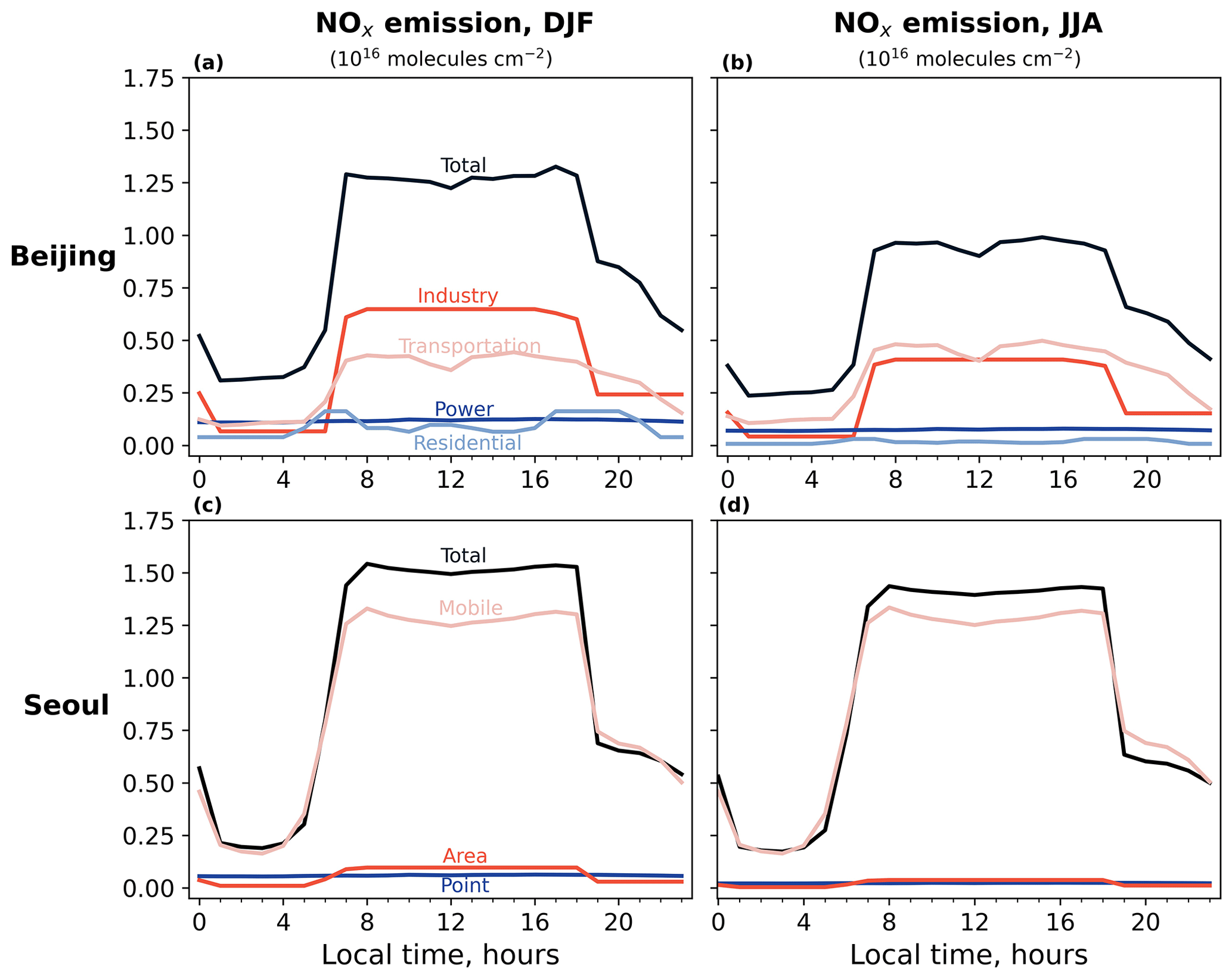
Figure 1Diurnal variation in NOx emissions in Beijing and Seoul for DJF 2021/22 and JJA 2022. Local time is Chinese standard time (CST) for Beijing and Korean standard time (KST) for Seoul. Solar noon is at 12:08–12:27 CST in Beijing and 12:21–12:45 KST in Seoul. Values are for the white boxes in Fig. 2. Different colors represent different sectors, and the black line shows the total emission.
Figure 1 shows that emissions are dominated by industrial and transport sources in Beijing and by mobile (transport) sources in Seoul. Both sectors show a broad maximum between 07:00 and 18:00 LT that defines the overall diurnal cycle of emissions and is similar in winter and summer. There are no significant rush hour peaks in transport emissions, suggesting that the surface NO2 maxima observed in early morning and evening are driven more by shallow mixing depths (Moutinho et al., 2020). Total NOx emission in Beijing in winter is 30 % greater than in summer, driven by the industrial source and possibly due to workplace heating. There is less seasonal variation in Seoul where mobile sources are the largest emitters.
Figure 2 shows the total NO2 columns over eastern China and South Korea observed by GEMS and simulated by GEOS-Chem during DJF 2021/22 and JJA 2022. The GEMS data are mapped on the 0.25° × 0.3125° GEOS-Chem grid. The yellow box delineates the Seoul Metropolitan Area (SMA). The zoomed-in black boxes are Beijing and Seoul, and the white boxes are the city centers where Pandora stations are located. The maximum NO2 concentrations are in the city centers in summer but are shifted to the south in winter due to the prevailing winds and the long NOx lifetime (Seo et al., 2021). We see from Fig. 2 that GEMS and GEOS-Chem have consistent spatial distributions and backgrounds, but GEOS-Chem over polluted regions is generally higher than GEMS except for Seoul in winter.
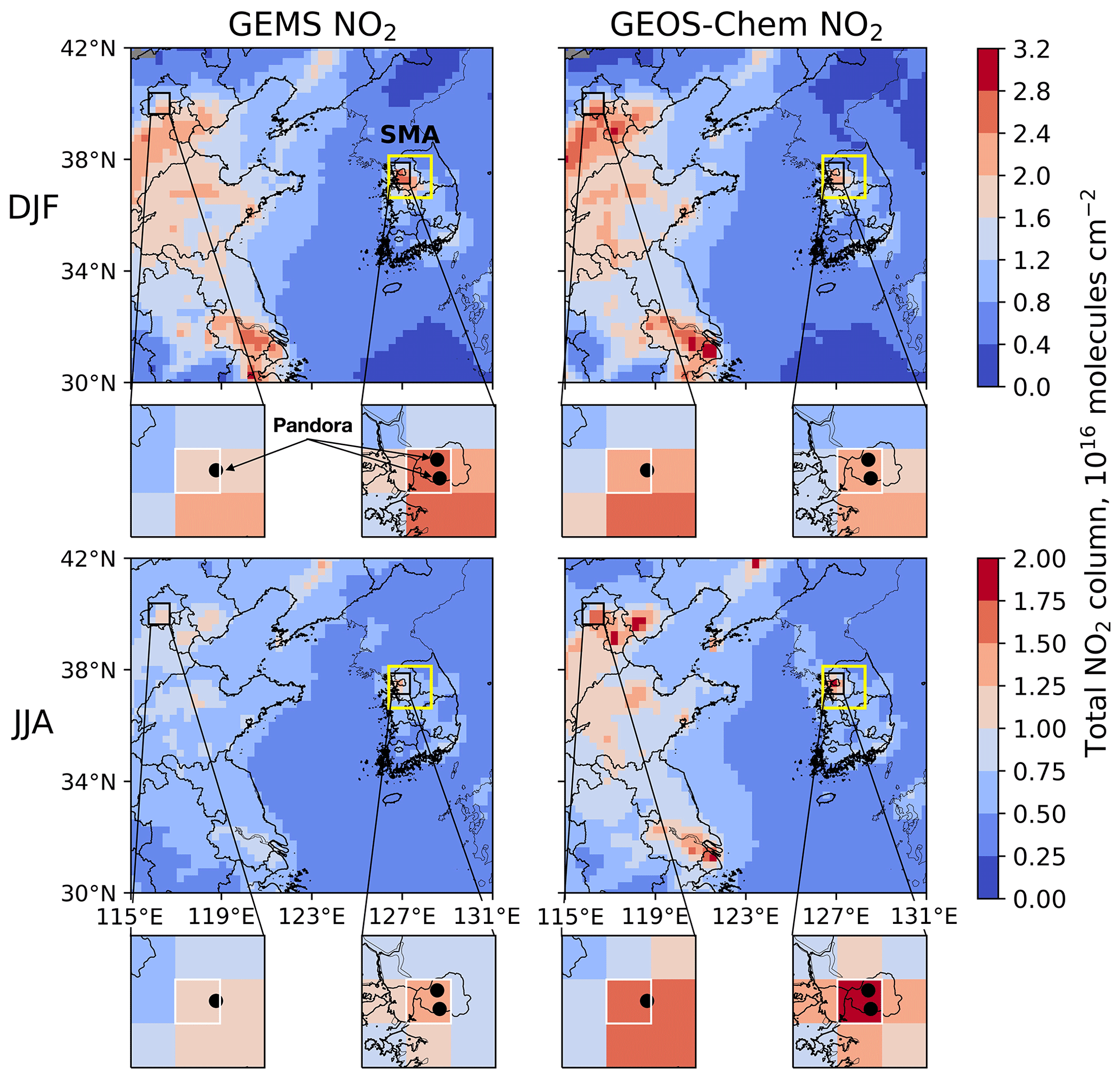
Figure 2Total NO2 columns over East Asia retrieved by GEMS and simulated by GEOS-Chem. The data are 3-month averages for December–July–February (DJF) 2021/22 and June–July–August (JJA) 2022 on the 0.25° × 0.3125° GEOS-Chem nested grid. The yellow rectangle delineates the Seoul Metropolitan Area (SMA; 36.6–38.1° N, 126.4–128.3° E). The zoomed-in plots show Beijing and Seoul, and the white boxes are the 0.25° × 0.3125° urban cores where the Pandora stations are located (black circles). Scales are different for DJF and JJA.
Figure 3 further intercompares GEOS-Chem and GEMS using the Pandora stations in Beijing and Seoul as evaluation metric. Previous GEMS evaluation with Pandora at the native pixel resolution of GEMS was presented by Kim et al. (2023). Here we conduct the evaluation on the coarser 0.25° × 0.3125° GEOS-Chem grid as most relevant for our work. GEMS and GEOS-Chem reproduce the diurnal and day-to-day variability observed by Pandora in DJF (R2= 0.87–0.90) and JJA (R2= 0.77–0.79). NO2 column magnitudes also agree well with Pandora in winter, with linear regression slopes of 0.94 for GEMS and 0.90 for GEOS-Chem. Summer shows larger biases, reflecting differences between the SNU and YSU Pandora sites that cannot be resolved at the 0.25° × 0.3125° resolution of GEOS-Chem (there are few observations at the Beijing site in JJA). YSU is more polluted than SNU, which is in a mountainous area more remote from emissions. Overall, a comparison to Pandora supports the diurnal and day-to-day variability seen in the GEMS and GEOS-Chem data. The rest of our analysis focuses on the diurnal variability.
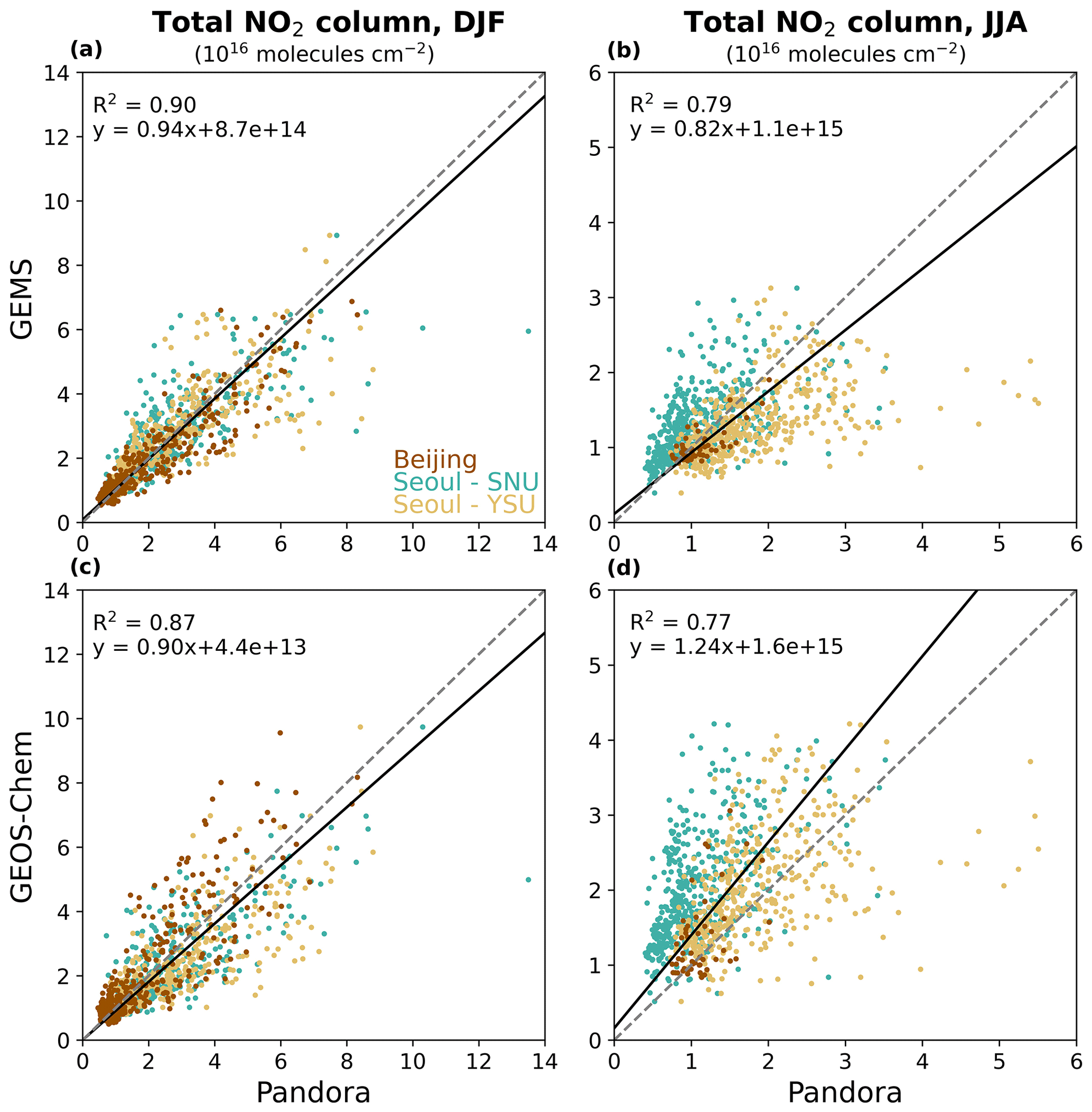
Figure 3Intercomparison of GEOS-Chem, GEMS, and Pandora NO2 columns for the Pandora sites in Beijing and Seoul. The figure shows scatterplots of daytime hourly data for DJF 2021/22 and JJA 2022. GEMS is mapped on the 0.25° × 0.3125° GEOS-Chem grid. Coefficients of determination (R2) and reduced major axis linear regressions are shown. The 1:1 line is dashed. The Beijing Pandora site has limited observations in JJA.
We start with an urban core analysis focusing on the white boxes shown in Fig. 2 for Beijing and Seoul, representing single 0.25° × 0.3125° GEOS-Chem grid cells where the Pandora stations are located. Scatterplot comparisons between GEOS-Chem, GEMS, and Pandora for these grid cells are shown in Fig. 3. Figure 4 shows the diurnal variation in the total NO2 column observed from GEMS and Pandora and simulated by GEOS-Chem in Beijing. GEOS-Chem results are shown as averages for all days and for the subset of days when GEMS observations are available (generally limited by cloud cover). Wintertime NO2 in all three datasets is flat from 10:00 to 11:00 LT and then increases from 11:00 to 14:00 LT. Summertime NO2 decreases from 08:00 LT to a minimum at 13:00–14:00 LT and then increases to 16:00 LT, consistent between GEOS-Chem and GEMS. Pandora observations in the summertime are too limited to show.
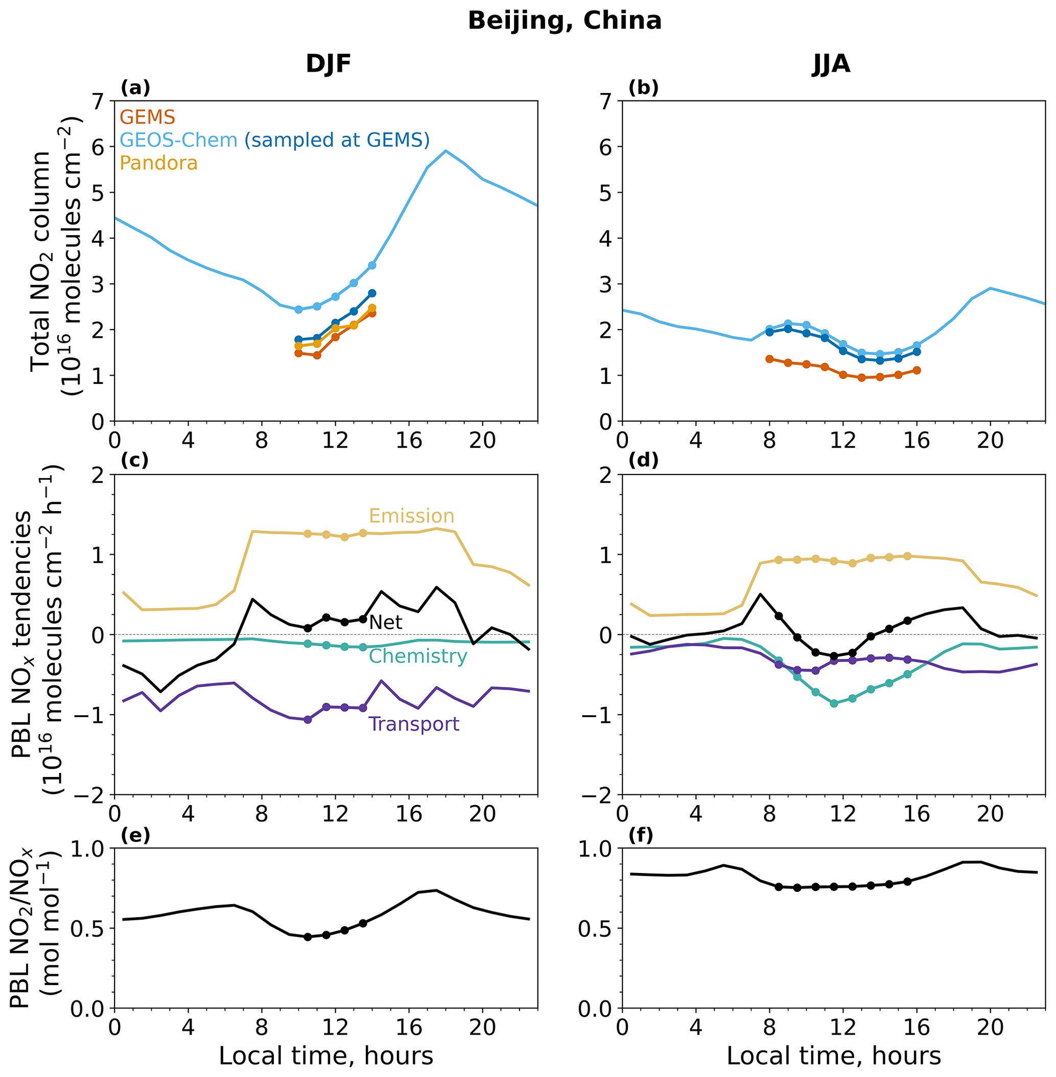
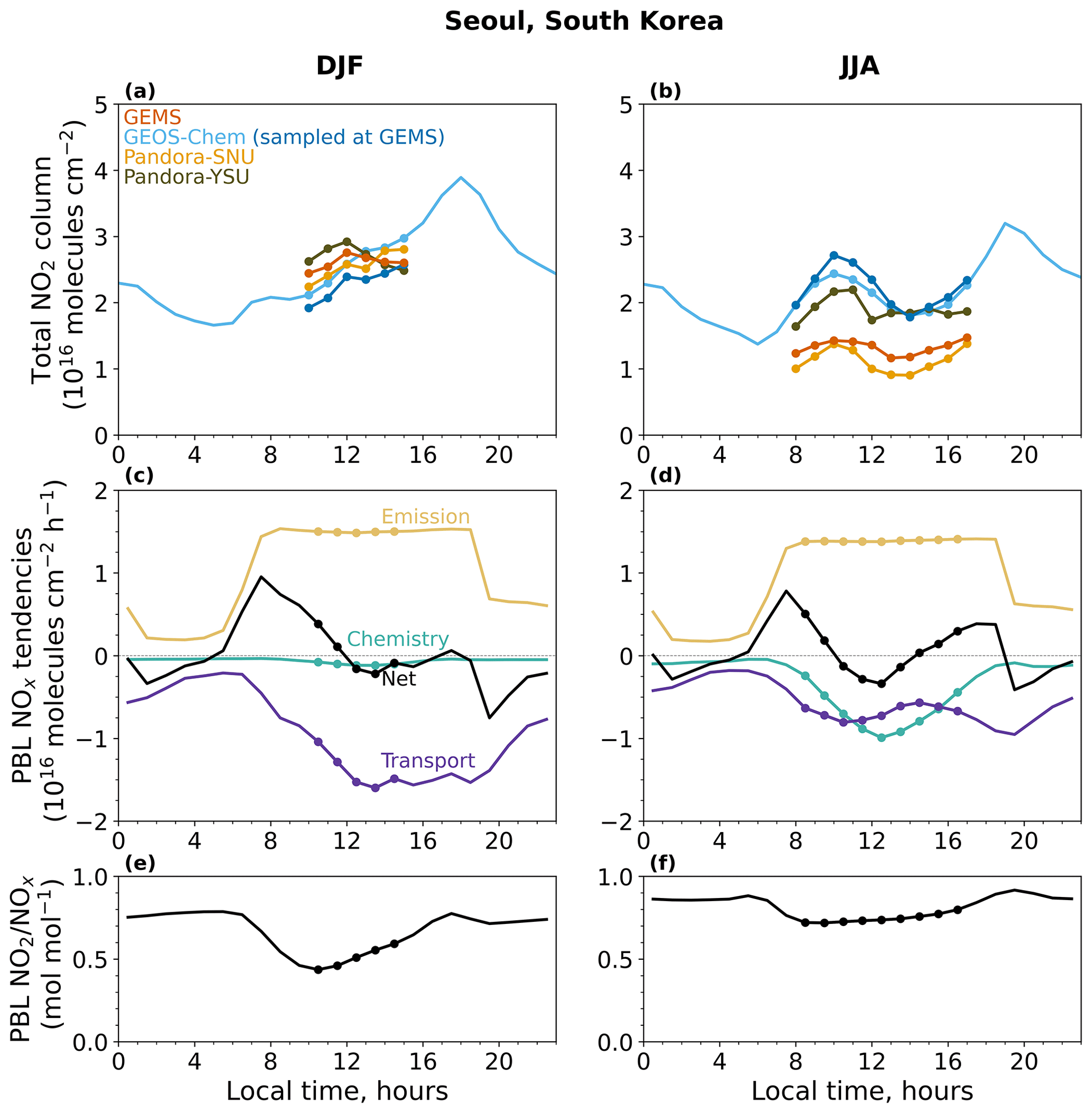
Figure 4Diurnal variation in total NO2 column and driving processes in Beijing. The first row shows the average NO2 columns observed by GEMS and Pandora and simulated by GEOS-Chem in DJF 2021/22 and JJA 2022 for the 0.25° × 0.3125° GEOS-Chem grid cell in the urban core where the Pandora station is located (white box in Fig. 2). GEMS observations are available for the hours indicated by symbols. GEOS-Chem results for the full diurnal cycle are shown as averages for all days and for the subset of days when GEMS data are available (generally limited by cloud cover). Pandora data are not shown for JJA due to a limited number of observations (Fig. 3). The second row shows the hourly tendencies in the GEOS-Chem NOx budget (averaged for all days) for the planetary boundary layer (PBL) conservatively defined as extending up to 3 km altitude. The tendencies describe the contributions from individual processes to the NOx budget as given by Eq. (3), with NOx defined as . The third row shows the PBL column molar ratio in GEOS-Chem.
We used the GEOS-Chem budget tendency diagnostic to understand the drivers of the diurnal variation in NO2 columns. This diagnostic tracks the mean mass-weighted changes in column concentrations after each model operation for any selected horizontal domain, vertical column, and time period. We focus on the PBL column conservatively defined as extending to 3 km altitude after verifying that altitudes higher than 3 km make negligible contributions to diurnal changes in the total model column. Within the PBL column we consider the budget of NO2 as that of NOx () multiplied by the local PBL column concentration ratio. This eliminates from the budget the fast interconversion reactions within the NOx family and provides a more useful budget perspective. It allows us to consider NOx emission as a source of NO2 even though NOx is emitted mainly as NO. The NOx family is mainly contributed by NO and NO2, and the main interconversion reactions defining the ratio are
where RO2 denotes organic peroxy radicals and X denotes halogen atoms. The net tendency for the PBL NO2 column (ΩNO2) can then be related to that of NOx () as
with
and where is the PBL column ratio. The terms on the right-hand side of Eq. (3) are updated by GEOS-Chem over its operator splitting time steps and are archived in the budget diagnostic as spatial and temporal averages. NOx dry deposition is included in the emission operator, but its contribution is very small (Shah et al., 2020). α(t) is archived every hour for application in Eq. (2).
The second row of Fig. 4 shows the different NOx budget terms from Eq. (3) over hourly time steps, with the net tendency as the left-hand-side term. The third row shows the PBL column molar ratios in GEOS-Chem. Each data point in the second and third rows (centered on the half hour) explains the change between the 2 successive hours shown in the first row. The GEOS-Chem diurnal variation in the NO2 column in the first row reflects the net NOx tendency combined with the ratio. We see that the increase in the NO2 column over the course of the day in winter reflects the dominant effect of daytime emissions, 4 times higher than at night and leading to NOx accumulation. Chemical loss is slow in winter, and transport (flux divergence) is the main loss term. The flat trend of the NO2 column from 10:00 to 11:00 LT corresponds to the diurnal minimum of the ratio. This ratio increases over the rest of the day as the mixed layer deepens and the freshly emitted NO is exposed to higher ozone concentrations. The increase in the ratio contributes to the increase in the NO2 column. The NO2 column in GEOS-Chem thus peaks at 18:00 LT. During the night, the NOx emission decreases, and the loss from transport leads to a decrease in the total NO2 column. The ratio at night is only 0.55 mol mol−1, despite no NO2 photolysis, because of sustained NO emission and the slow rate of the NO+O3 reaction (low ozone and low temperatures).
The opposite diurnal variation in NO2 in summer reflects weaker daytime emission of NOx and stronger chemical loss as shown by the GEOS-Chem budget analysis. Even though the emission term remains larger than the chemical loss term, there is also a negative transport term from ventilation. The chemical loss of NOx peaks at 11:00–12:00 LT and then weakens, reflecting the noon maximum of OH concentrations (Logan et al., 1981) combined with the decreasing NO2 concentration and explaining the slow recovery of the NO2 column in the afternoon. The ratio is higher in summer than in winter and shows little variation during the daytime, reflecting the higher concentrations of O3 and HO2 radicals offsetting the effect of NO2 photolysis. The daytime ratio averages 0.75 mol mol−1 in summer, as compared to 0.50 mol mol−1 in winter, contributing to the seasonality of NO2 seen from space.
Figure 5 shows the same as Fig. 4 but for Seoul. The two Pandora stations show differences in NO2 columns, particularly in summer, as previously shown in Fig. 3. They also show some differences in diurnal variation, particularly in winter, which we similarly attribute to local effects such as different emissions, wind speeds, and geography that cannot be resolved at 25 km resolution. The diurnal variations in GEMS and GEOS-Chem agree to within the ranges defined by data from the two Pandora stations. NO2 columns in winter increase from 10:00 to 12:00 LT as in Beijing but then flatten in the afternoon, which we attribute in GEOS-Chem to stronger winds. NO2 columns in summer show an increase from 08:00 to 10:00 LT, unlike in Beijing, because of larger emissions initially overwhelming the chemical loss term. There follows a decrease until 13:00–14:00 LT and a recovery in the later afternoon, similar to Beijing and driven by the same factors.
We showed in Sect. 4 that the diurnal variation in the NO2 column observed by GEMS on the urban scale reflects a balance between emission and transport in winter, as well as the added influence from chemical loss in summer. The transport term can be represented with a CTM in an inversion framework (Cooper et al., 2017), but simple quantification of the transport term on the urban scale can also be done from knowledge of the wind speed with a mass balance approach (Jacob et al., 2016).
Figure 6 illustrates the sensitivity of the NO2 diurnal variation to wind speed in the wintertime GEMS observations over Seoul when chemical loss is a negligible term. A wind speed of 6 m s−1 ventilates the 25 × 25 km2 urban core on a timescale of 1 h. Here we segregate the data by GEOS-FP hourly wind speed at 850 hPa higher or lower than 6 m s−1. The diurnal variations are very different at high and low wind speed and consistent between GEMS and GEOS-Chem. At high wind speed, the NO2 column shows little diurnal variability because emission is balanced by transport. At low wind speed, NO2 accumulates over the daytime hours because the transport term is weaker and does not keep up with emissions. Steady state between emissions and ventilation is finally reached at 16:00 LT, but the NO2 column keeps increasing until 18:00 LT because of increasing ratio. Edwards et al. (2024) found an anticorrelation between the wind speed and tropospheric NO2 column concentrations consistent with our findings.
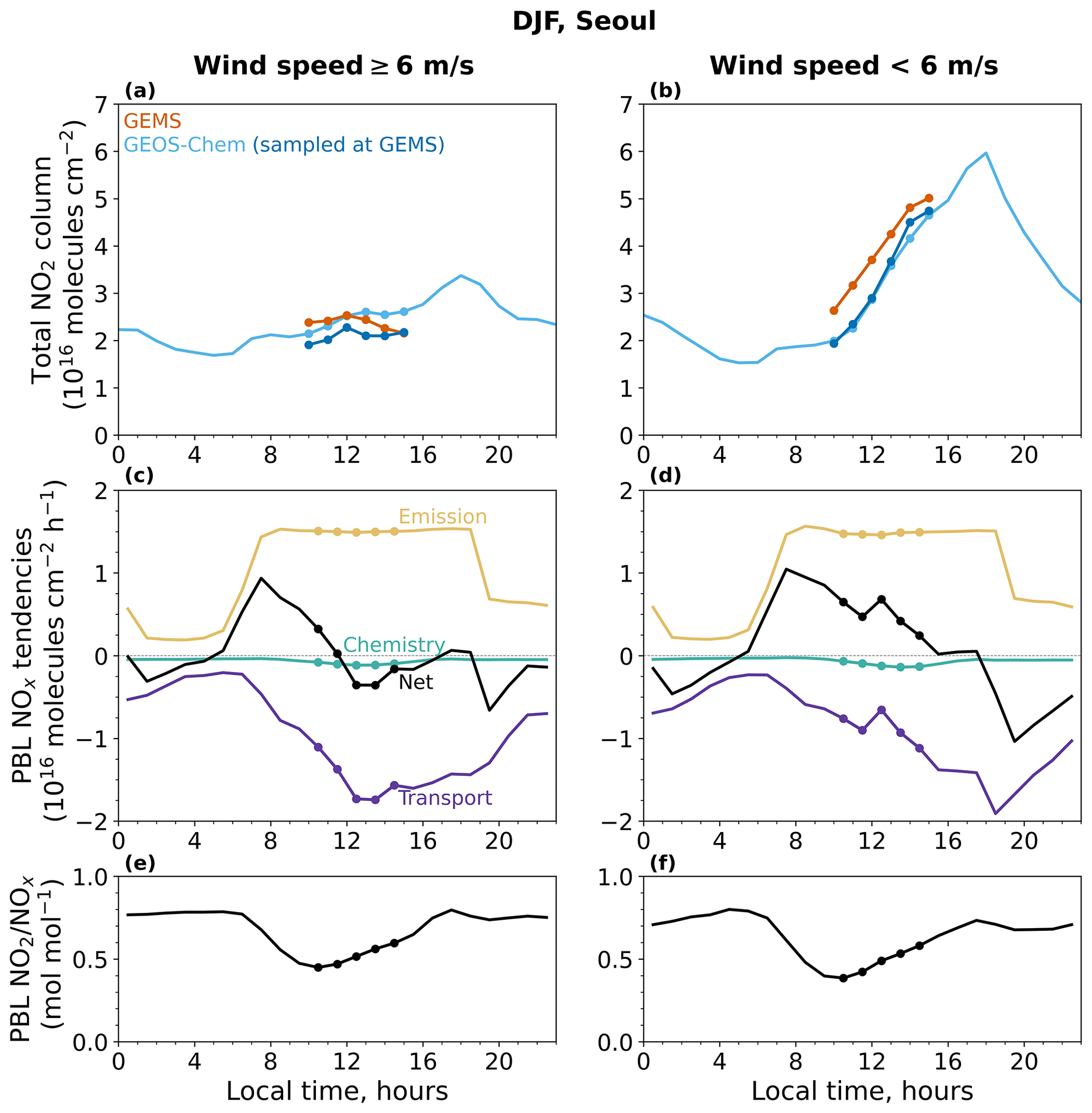
Figure 6Same as Fig. 4 but for DJF 2021/22 in Seoul with data segregated by wind speed. Segregation threshold is 6 m s−1 for the 850 hPa hourly wind speed in the NASA GEOS-FP meteorological data used as input to GEOS-Chem.
One can reduce the effect of transport by spatial averaging over a large domain, thereby increasing the ventilation timescale. Edwards et al. (2024) showed that regionally averaging the data over northeast Asia minimized the transport effect, though the interpretation of the result is more complicated due to averaging over diverse emission and chemical environments. Figure 7 shows the average diurnal pattern of the NO2 column observed by GEMS and simulated by GEOS-Chem on the ≈ 150 km scale of the SMA (Fig. 2) in winter and summer. Again, the diurnal variations observed by GEMS and simulated by GEOS-Chem are consistent. NO2 columns in winter increase over the course of the day in a more regular manner than on the 25 km urban scale (Fig. 5a) because the transport loss term is steadier and responds mainly to the change in the NO2 column. The chemical loss term is not negligible, unlike on the urban scale, because its timescale of about 20 h is comparable to that of transport.
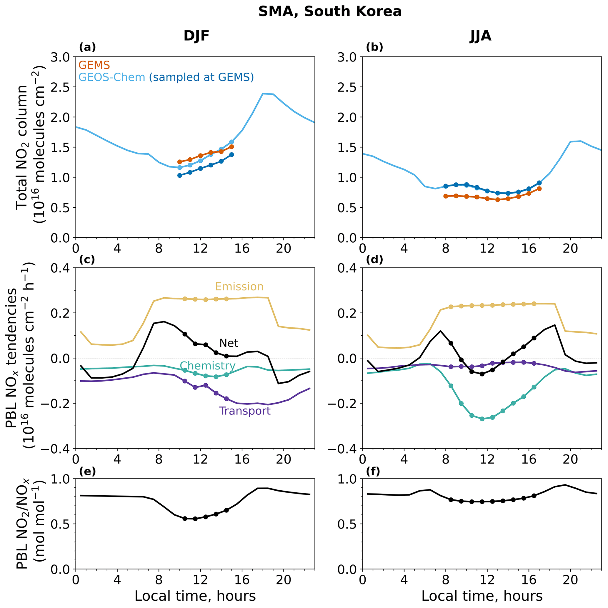
Figure 7Same as for Fig. 4 but for the Seoul Metropolitan Area (SMA; 36.6–38.1° N, 126.4–128.3° E) corresponding to the yellow box in Fig. 2. Quantities are averages over all 0.25° × 0.3125° grid cells in the SMA.
We see from Fig. 7 that the transport term can be successfully marginalized on the scale of the SMA in summer because the chemical loss term is faster. The resulting SMA diurnal pattern of the total NO2 column is consistent with that of Seoul (Fig. 5b) but with a flatter shape, and the early-afternoon minimum is now driven mainly by chemistry. The amplitude is greatly dampened because emissions are 5 times weaker when averaged over the SMA regional domain and because the chemical loss integrates over the residence time within the domain.
We used the GEOS-Chem model to interpret the diurnal variation in NO2 columns observed from the GEMS geostationary instrument and Pandora ground-based spectrometers over Beijing and Seoul in December–January–February (DJF) 2021/22 and June–July–August (JJA) 2022. This was motivated by the need to understand the unique information offered by hourly geostationary satellite observations on the budget of NOx through the contributions of emissions, chemistry, and transport to the diurnal cycle of NO2.
The GEOS-Chem model used in this work had previously shown successful simulation of the NO2 vertical profile and its diurnal variation over Seoul in the KORUS-AQ aircraft campaign, enabling reliable computation of the diurnal dependence of the air mass factor (AMF) that contributes to the diurnal variation in NO2 observed from space. Here we used the diagnostic budget capability in GEOS-Chem to isolate the contributions of NOx emissions, chemistry, transport, and the column ratio to the diurnal cycle of NO2 columns. We also updated NOx emissions to 2022 including their diurnal variations. The NOx emissions for Beijing and Seoul are a factor of 4 higher in the daytime than at night, reflecting mobile and industrial sources, and show little variation during the daytime hours. We focused on the simulation of the total atmospheric NO2 column rather than the tropospheric column, taking advantage of the stratospheric capability in GEOS-Chem, to avoid errors in the definition of the tropopause. Diurnal variation in the NO2 atmospheric column in the two cities is mainly determined by the planetary boundary layer (PBL) up to 3 km altitude.
We investigated the diurnal variation in the NO2 column at the 25 km urban scale over Beijing and Seoul. GEMS, Pandora, and GEOS-Chem show similar variability and diurnal variations. NO2 columns in winter increase over the course of the daytime hours, reflecting accumulation from high daytime emissions offset by loss from horizontal transport (flux divergence), and are further enhanced by an increase in the over the course of the day as ozone is entrained in the growing mixed layer. Chemical loss of NOx in winter is too slow to play a significant role in the observed diurnal variation. In summer, by contrast, NO2 columns decrease from 10:00 to 14:00 LT because of NOx photochemical oxidation compounding the loss from transport.
We further examined the importance of transport for interpreting the diurnal variation in the GEMS urban NO2 data by segregating the Seoul data by wind speed. In winter, the low-wind GEMS data (< 6 m s−1) show a steady rise in NO2 over the course of the day, while the high-wind data (≥ 6 m s−1) show flat diurnal variation, consistent with the GEOS-Chem model. Transport plays an important role in the NOx budget in both cases but cannot keep up with the high daytime emissions in the low-wind case.
We examined whether the role of transport in the diurnal variation in the urban NO2 column could be reduced by spatial averaging of the data over the 150 km regional scale of the Seoul Metropolitan Area (SMA). The SMA data in winter show a steady increase over the daytime hours due to emissions, but the transport term remains the major sink of NOx. The SMA data in summer show negligible loss from transport in daytime because the chemical loss term is much faster, but the diurnal amplitude is weak because of diluted emissions and long residence times for the air over the regional domain.
Our conclusions regarding the interpretation of the diurnal variation in NO2 columns observed by GEMS can be extended to other instruments of the geostationary air quality constellation, such as TEMPO over North America, launched in April 2023, and Sentinel-4 over Europe, scheduled for launch in 2024. This work further lays the groundwork for the use of GEOS-Chem in inversions of the geostationary satellite data to infer NOx emissions.
The model code used in this work is available at https://doi.org/10.5281/zenodo.5764874 (The International GEOS-Chem User Community, 2021).
The GEMS L2 NO2 version 2.0 slant column data can be obtained from https://nesc.nier.go.kr/ (NIER, 2023). The total NO2 columns from Pandora are available from the Pandonia Global Network website (http://pandonia-global-network.org; PGN, 2023). The surface NO2 data over China are available from https://quotsoft.net/air/ (MEE, 2023). The surface NO2 data over South Korea are from the AirKorea website (https://www.airkorea.or.kr/web/last_amb_hour_data?pMENU_NO=123; KEC, 2022). The Seoul hourly traffic count data are available from the Seoul Transport Operation and Information Services website (https://topis.seoul.go.kr/; TOPIS, 2023).
The original draft preparation was done by LHY, with review and editing by DJJ, KRT, JHC, HL, and JK. DJJ contributed to project conceptualization. Modeling was done by LHY with additional support from HPL, NKC, SZ, VS, EB, XF, RMY, and DCP. The formal analysis was conducted by LHY with additional support from DJJ, RD, YJO, HC, JP, HLL, WJL, SK, EK, KRT, and JHC.
The contact author has declared that none of the authors has any competing interests.
Publisher's note: Copernicus Publications remains neutral with regard to jurisdictional claims made in the text, published maps, institutional affiliations, or any other geographical representation in this paper. While Copernicus Publications makes every effort to include appropriate place names, the final responsibility lies with the authors.
This material is based upon work supported by the National Science Foundation Graduate Research Fellowship under grant no. DGE 2140743. We thank A. G. Russell for helpful discussions.
This research has been supported by the Samsung Advanced Institute of Technology (grant no. A41602) and the Harvard–NUIST Joint Laboratory for Air Quality and Climate.
This paper was edited by Bryan N. Duncan and reviewed by Josh Laughner and one anonymous referee.
Bae, M., Yoo, C., Kim, H., and Kim, S.: Developing Temporal Allocation Profiles for Electric Generating Utilities based on the CleanSYS Real-time Emissions, Journal of Korean Society for Atmospheric Environment, 37, 338–354, https://doi.org/10.5572/KOSAE.2021.37.2.338, 2021.
Boersma, K. F., Jacob, D. J., Eskes, H. J., Pinder, R. W., Wang, J., and van der A, R. J.: Intercomparison of SCIAMACHY and OMI tropospheric NO2 columns: Observing the diurnal evolution of chemistry and emissions from space, J. Geophys. Res., 113, D16S26, https://doi.org/10.1029/2007JD008816, 2008.
Boersma, K. F., Jacob, D. J., Trainic, M., Rudich, Y., DeSmedt, I., Dirksen, R., and Eskes, H. J.: Validation of urban NO2 concentrations and their diurnal and seasonal variations observed from the SCIAMACHY and OMI sensors using in situ surface measurements in Israeli cities, Atmos. Chem. Phys., 9, 3867–3879, https://doi.org/10.5194/acp-9-3867-2009, 2009.
Chang, L.-S., Kim, D., Hong, H., Kim, D.-R., Yu, J.-A., Lee, K., Lee, H., Kim, D., Hong, J., Jo, H.-Y., and Kim, C.-H.: Evaluation of correlated Pandora column NO2 and in situ surface NO2 measurements during GMAP campaign, Atmos. Chem. Phys., 22, 10703–10720, https://doi.org/10.5194/acp-22-10703-2022, 2022.
Cheng, N., Li, Y., Sun, F., Chen, C., Wang, B., Li, Q., Wei, P., and Cheng, B.: Ground-Level NO2 in Urban Beijing: Trends, Distribution, and Effects of Emission Reduction Measures, Aerosol Air Qual. Res., 18, 343–356, https://doi.org/10.4209/aaqr.2017.02.0092, 2018.
Cooper, M., Martin, R. V., Padmanabhan, A., and Henze, D. K.: Comparing mass balance and adjoint methods for inverse modeling of nitrogen dioxide columns for global nitrogen oxide emissions, J. Geophys. Res.-Atmos., 122, 4718–4734, https://doi.org/10.1002/2016JD025985, 2017.
Crawford, J. H., Ahn, J.-Y., Al-Saadi, J., Chang, L., Emmons, L. K., Kim, J., Lee, G., Park, J.-H., Park, R. J., Woo, J. H., Song, C.-K., Hong, J.-H., Hong, Y.-D., Lefer, B. L., Lee, M., Lee, T., Kim, S., Min, K.-E., Yum, S. S., Shin, H. J., Kim, Y.-W., Choi, J.-S., Park, J.-S., Szykman, J. J., Long, R. W., Jordan, C. E., Simpson, I. J., Fried, A., Dibb, J. E., Cho, S., and Kim, Y. P.: The Korea–United States Air Quality (KORUS-AQ) field study, Elementa: Science of the Anthropocene, 9, 00163, https://doi.org/10.1525/elementa.2020.00163, 2021.
Edwards, D. P., Martínez-Alonso, S., Jo, D. S., Ortega, I., Emmons, L. K., Orlando, J. J., Worden, H. M., Kim, J., Lee, H., Park, J., and Hong, H.: Quantifying the diurnal variation of atmospheric NO2 from observations of the Geostationary Environment Monitoring Spectrometer (GEMS), EGUsphere [preprint], https://doi.org/10.5194/egusphere-2024-570, 2024.
Ghude, S. D., Karumuri, R. K., Jena, C., Kulkarni, R., Pfister, G. G., Sajjan, V. S., Pithani, P., Debnath, S., Kumar, R., Upendra, B., Kulkarni, S. H., Lal, D. M., Vander A, R. J., and Mahajan, A. S.: What is driving the diurnal variation in tropospheric NO2 columns over a cluster of high emission thermal power plants in India?, Atmospheric Environment: X, 5, 100058, https://doi.org/10.1016/j.aeaoa.2019.100058, 2020.
Gulde, S. T., Kolm, M. G., Smith, D. J., Maurer, R., Courrèges-Lacoste, G. B., Sallusti, M., and Bagnasco, G.: Sentinel 4: a geostationary imaging UVN spectrometer for air quality monitoring: status of design, performance and development, in: International Conference on Space Optics – ICSO 2014, Tenerife, Spain, 17 November 2017, SPIE, 1158–1166, https://doi.org/10.1117/12.2304099, 2017.
Herman, J., Cede, A., Spinei, E., Mount, G., Tzortziou, M., and Abuhassan, N.: NO2 column amounts from ground-based Pandora and MFDOAS spectrometers using the direct-sun DOAS technique: Intercomparisons and application to OMI validation, J. Geophys. Res., 114, D13307, https://doi.org/10.1029/2009JD011848, 2009.
Herman, J., Spinei, E., Fried, A., Kim, J., Kim, J., Kim, W., Cede, A., Abuhassan, N., and Segal-Rozenhaimer, M.: NO2 and HCHO measurements in Korea from 2012 to 2016 from Pandora spectrometer instruments compared with OMI retrievals and with aircraft measurements during the KORUS-AQ campaign, Atmos. Meas. Tech., 11, 4583–4603, https://doi.org/10.5194/amt-11-4583-2018, 2018.
Judd, L. M., Al-Saadi, J. A., Szykman, J. J., Valin, L. C., Janz, S. J., Kowalewski, M. G., Eskes, H. J., Veefkind, J. P., Cede, A., Mueller, M., Gebetsberger, M., Swap, R., Pierce, R. B., Nowlan, C. R., Abad, G. G., Nehrir, A., and Williams, D.: Evaluating Sentinel-5P TROPOMI tropospheric NO2 column densities with airborne and Pandora spectrometers near New York City and Long Island Sound, Atmos. Meas. Tech., 13, 6113–6140, https://doi.org/10.5194/amt-13-6113-2020, 2020.
Jacob, D. J., Turner, A. J., Maasakkers, J. D., Sheng, J., Sun, K., Liu, X., Chance, K., Aben, I., McKeever, J., and Frankenberg, C.: Satellite observations of atmospheric methane and their value for quantifying methane emissions, Atmos. Chem. Phys., 16, 14371–14396, https://doi.org/10.5194/acp-16-14371-2016, 2016.
Kanaya, Y., Irie, H., Takashima, H., Iwabuchi, H., Akimoto, H., Sudo, K., Gu, M., Chong, J., Kim, Y. J., Lee, H., Li, A., Si, F., Xu, J., Xie, P.-H., Liu, W.-Q., Dzhola, A., Postylyakov, O., Ivanov, V., Grechko, E., Terpugova, S., and Panchenko, M.: Long-term MAX-DOAS network observations of NO2 in Russia and Asia (MADRAS) during the period 2007–2012: instrumentation, elucidation of climatology, and comparisons with OMI satellite observations and global model simulations, Atmos. Chem. Phys., 14, 7909–7927, https://doi.org/10.5194/acp-14-7909-2014, 2014.
KEC (Korea Environment Corporation): NO2 dataset in South Korea, KEC [data set], https://www.airkorea.or.kr/web/last_amb_hour_data?pMENU_NO=123 (last access: 14 June 2024), 2022.
Kendrick, C. M., Koonce, P., and George, L. A.: Diurnal and seasonal variations of NO, NO2 and PM2.5 mass as a function of traffic volumes alongside an urban arterial, Atmos. Environ., 122, 133–141, https://doi.org/10.1016/j.atmosenv.2015.09.019, 2015.
Kim, H. C., Kim, S., Lee, S.-H., Kim, B.-U., and Lee, P.: Fine-Scale Columnar and Surface NOx Concentrations over South Korea: Comparison of Surface Monitors, TROPOMI, CMAQ and CAPSS Inventory, Atmosphere, 11, 101, https://doi.org/10.3390/atmos11010101, 2020.
Kim, J., Kim, J., Cho, H.-K., Herman, J., Park, S. S., Lim, H. K., Kim, J.-H., Miyagawa, K., and Lee, Y. G.: Intercomparison of total column ozone data from the Pandora spectrophotometer with Dobson, Brewer, and OMI measurements over Seoul, Korea, Atmos. Meas. Tech., 10, 3661–3676, https://doi.org/10.5194/amt-10-3661-2017, 2017.
Kim, J., Jeong, U., Ahn, M.-H., Kim, J. H., Park, R. J., Lee, H., Song, C. H., Choi, Y.-S., Lee, K.-H., Yoo, J.-M., Jeong, M.-J., Park, S. K., Lee, K.-M., Song, C.-K., Kim, S.-W., Kim, Y. J., Kim, S.-W., Kim, M., Go, S., Liu, X., Chance, K., Chan Miller, C., Al-Saadi, J., Veihelmann, B., Bhartia, P. K., Torres, O., Abad, G. G., Haffner, D. P., Ko, D. H., Lee, S. H., Woo, J.-H., Chong, H., Park, S. S., Nicks, D., Choi, W. J., Moon, K.-J., Cho, A., Yoon, J., Kim, S., Hong, H., Lee, K., Lee, H., Lee, S., Choi, M., Veefkind, P., Levelt, P. F., Edwards, D. P., Kang, M., Eo, M., Bak, J., Baek, K., Kwon, H.-A., Yang, J., Park, J., Han, K. M., Kim, B.-R., Shin, H.-W., Choi, H., Lee, E., Chong, J., Cha, Y., Koo, J.-H., Irie, H., Hayashida, S., Kasai, Y., Kanaya, Y., Liu, C., Lin, J., Crawford, J. H., Carmichael, G. R., Newchurch, M. J., Lefer, B. L., Herman, J. R., Swap, R. J., Lau, A. K. H., Kurosu, T. P., Jaross, G., Ahlers, B., Dobber, M., McElroy, C. T., and Choi, Y.: New Era of Air Quality Monitoring from Space: Geostationary Environment Monitoring Spectrometer (GEMS), B. Am. Meteorol. Soc., 101, E1–E22, https://doi.org/10.1175/BAMS-D-18-0013.1, 2020.
Kim, M.-H., Yeo, H., Park, S., Park, D.-H., Omar, A., Nishizawa, T., Shimizu, A., and Kim, S.-W.: Assessing CALIOP-Derived Planetary Boundary Layer Height Using Ground-Based Lidar, Remote Sens., 13, 1496, https://doi.org/10.3390/rs13081496, 2021.
Kim, S., Kim, D., Hong, H., Chang, L.-S., Lee, H., Kim, D.-R., Kim, D., Yu, J.-A., Lee, D., Jeong, U., Song, C.-K., Kim, S.-W., Park, S. S., Kim, J., Hanisco, T. F., Park, J., Choi, W., and Lee, K.: First-time comparison between NO2 vertical columns from Geostationary Environmental Monitoring Spectrometer (GEMS) and Pandora measurements, Atmos. Meas. Tech., 16, 3959–3972, https://doi.org/10.5194/amt-16-3959-2023, 2023.
Lange, K., Richter, A., Bösch, T., Zilker, B., Latsch, M., Behrens, L. K., Okafor, C. M., Bösch, H., Burrows, J. P., Merlaud, A., Pinardi, G., Fayt, C., Friedrich, M. M., Dimitropoulou, E., Van Roozendael, M., Ziegler, S., Ripperger-Lukosiunaite, S., Kuhn, L., Lauster, B., Wagner, T., Hong, H., Kim, D., Chang, L.-S., Bae, K., Song, C.-K., and Lee, H.: Validation of GEMS tropospheric NO2 columns and their diurnal variation with ground-based DOAS measurements, EGUsphere [preprint], https://doi.org/10.5194/egusphere-2024-617, 2024.
Lee, H., Park, J., and Hyunkee, H.: Geostationary Environment Monitoring Spectrometer (GEMS) User's Guide – Nitrogen Dioxide, The National Institute of Environmental Research, Republic of Korea, https://nesc.nier.go.kr/ko/html/satellite/guide/guide.do (last access: 11 June 2024), 2020.
Liu, M., Lin, J., Wang, Y., Sun, Y., Zheng, B., Shao, J., Chen, L., Zheng, Y., Chen, J., Fu, T.-M., Yan, Y., Zhang, Q., and Wu, Z.: Spatiotemporal variability of NO2 and PM2.5 over Eastern China: observational and model analyses with a novel statistical method, Atmos. Chem. Phys., 18, 12933–12952, https://doi.org/10.5194/acp-18-12933-2018, 2018.
Liu, O., Li, Z., Lin, Y., Fan, C., Zhang, Y., Li, K., Zhang, P., Wei, Y., Chen, T., Dong, J., and de Leeuw, G.: Evaluation of the first year of Pandora NO2 measurements over Beijing and application to satellite validation, Atmos. Meas. Tech., 17, 377–395, https://doi.org/10.5194/amt-17-377-2024, 2024.
Liu, X., Gao, X., Wu, X., Yu, W., Chen, L., Ni, R., Zhao, Y., Duan, H., Zhao, F., Chen, L., Gao, S., Xu, K., Lin, J., and Ku, A. Y.: Updated Hourly Emissions Factors for Chinese Power Plants Showing the Impact of Widespread Ultralow Emissions Technology Deployment, Environ. Sci. Technol., 53, 2570–2578, https://doi.org/10.1021/acs.est.8b07241, 2019.
Logan, J., Prather, M. J., Wofsy, F. C., and McElroy, M. B.: Tropospheric chemistry: A global perspective, J. Geophys. Res.-Oceans, 86, 7210–7254, https://doi.org/10.1029/JC086iC08p07210, 1981.
Martin, R. V., Chance, K., Jacob, D. J., Kurosu, T. P., Spurr, R. J. D., Bucsela, E., Gleason, J. F., Palmer, P. I., Bey, I., Fiore, A. M., Li, Q., Yantosca, R. M., and Koelemeijer, R. B. A.: An improved retrieval of tropospheric nitrogen dioxide from GOME, J. Geophys. Res., 107, 4437, https://doi.org/10.1029/2001JD001027, 2002.
MEE (The Ministry of Ecology and Environment): NO2 dataset in China, MEE [data set], https://quotsoft.net/air/ (last access: 11 June 2024), 2023.
Miao, R., Chen, Q., Zheng, Y., Cheng, X., Sun, Y., Palmer, P. I., Shrivastava, M., Guo, J., Zhang, Q., Liu, Y., Tan, Z., Ma, X., Chen, S., Zeng, L., Lu, K., and Zhang, Y.: Model bias in simulating major chemical components of PM2.5 in China, Atmos. Chem. Phys., 20, 12265–12284, https://doi.org/10.5194/acp-20-12265-2020, 2020.
Moutinho, J. L., Liang, D., Golan, R., Sarnat, S. E., Weber, R., Sarnat, J. A., and Russell, A. G.: Near-road vehicle emissions air quality monitoring for exposure modeling, Atmos. Environ., 224, 117318, https://doi.org/10.1016/j.atmosenv.2020.117318, 2020.
NIER (The National Institute of Environmental Research): GEMS dataset, NIER, Republic of South Korea, https://nesc.nier.go.kr/ (last access: 11 June 2024), 2023.
Oak, Y. J., Jacob, D. J., Balasus, N., Yang, L. H., Chong, H., Park, J., Lee, H., Lee, G. T., Ha, E. S., Park, R. J., Kwon, H.-A., and Kim, J.: A bias-corrected GEMS geostationary satellite product for nitrogen dioxide using machine learning to enforce consistency with the TROPOMI satellite instrument, EGUsphere [preprint], https://doi.org/10.5194/egusphere-2024-393, 2024.
Palmer, P. I., Jacob, D. J., Chance, K., Martin, R. V., Spurr, R. J. D., Kurosu, T. P., Bey, I., Yantosca, R., Fiore, A., and Li, Q.: Air mass factor formulation for spectroscopic measurements from satellites: Application to formaldehyde retrievals from the Global Ozone Monitoring Experiment, J. Geophys. Res., 106, 14539–14550, https://doi.org/10.1029/2000JD900772, 2001.
Park, R. J. and Kwon, H.-A.: Algorithm Theoretical Basis Document – VOC (HCHO/CHOCHO) Retrieval Algorithm, The National Institute of Environmental Research, Republic of Korea, https://nesc.nier.go.kr/en/html/satellite/doc/doc.do (last access: 11 June 2024), 2020.
Park, R. J., Oak, Y. J., Emmons, L. K., Kim, C.-H., Pfister, G. G., Carmichael, G. R., Saide, P. E., Cho, S.-Y., Kim, S., Woo, J.-H., Crawford, J. H., Gaubert, B., Lee, H.-J., Park, S.-Y., Jo, Y.-J., Gao, M., Tang, B., Stanier, C. O., Shin, S. S., Park, H. Y., Bae, C., and Kim, E.: Multi-model intercomparisons of air quality simulations for the KORUS-AQ campaign, Elementa: Science of the Anthropocene, 9, 00139, https://doi.org/10.1525/elementa.2021.00139, 2021.
Park, S., Kim, S.-W., Park, M.-S., and Song, C.-K.: Measurement of Planetary Boundary Layer Winds with Scanning Doppler Lidar, Remote Sens., 10, 1261, https://doi.org/10.3390/rs10081261, 2018.
Penn, E. and Holloway, T.: Evaluating current satellite capability to observe diurnal change in nitrogen oxides in preparation for geostationary satellite missions, Environ. Res. Lett., 15, 034038, https://doi.org/10.1088/1748-9326/ab6b36, 2020.
PGN: Pandonia Global Network (PGN) data products readme document, https://www.pandonia-global-network.org/wp-content/uploads/2021/01/PGN_DataProducts_Readme_v1-8-3.pdf (last access: 11 June 2024), 2021.
PGN: Pandonia Global Network (PGN) data archive, PGN, http://data.pandonia-global-network.org/ (last access: 11 June 2024), 2023.
Seo, S., Kim, S.-W., Kim, K.-M., Lamsal, L. N., and Jin, H.: Reductions in NO2 concentrations in Seoul, South Korea detected from space and ground-based monitors prior to and during the COVID-19 pandemic, Environ. Res. Commun., 3, 051005, https://doi.org/10.1088/2515-7620/abed92, 2021.
Shah, V., Jacob, D. J., Li, K., Silvern, R. F., Zhai, S., Liu, M., Lin, J., and Zhang, Q.: Effect of changing NOx lifetime on the seasonality and long-term trends of satellite-observed tropospheric NO2 columns over China, Atmos. Chem. Phys., 20, 1483–1495, https://doi.org/10.5194/acp-20-1483-2020, 2020.
The International GEOS-Chem User Community: geoschem/GC-Classic: GEOS-Chem 13.3.4, Version 13.3.4, Zenodo [code], https://doi.org/10.5281/zenodo.5764874, 2021.
TOPIS: Seoul Transport Operation and Information Services (TOPIS) Seoul traffic count data, TOPIS, https://topis.seoul.go.kr/ (last access: 11 June 2024), 2023.
Verhoelst, T., Compernolle, S., Pinardi, G., Lambert, J.-C., Eskes, H. J., Eichmann, K.-U., Fjæraa, A. M., Granville, J., Niemeijer, S., Cede, A., Tiefengraber, M., Hendrick, F., Pazmiño, A., Bais, A., Bazureau, A., Boersma, K. F., Bognar, K., Dehn, A., Donner, S., Elokhov, A., Gebetsberger, M., Goutail, F., Grutter de la Mora, M., Gruzdev, A., Gratsea, M., Hansen, G. H., Irie, H., Jepsen, N., Kanaya, Y., Karagkiozidis, D., Kivi, R., Kreher, K., Levelt, P. F., Liu, C., Müller, M., Navarro Comas, M., Piters, A. J. M., Pommereau, J.-P., Portafaix, T., Prados-Roman, C., Puentedura, O., Querel, R., Remmers, J., Richter, A., Rimmer, J., Rivera Cárdenas, C., Saavedra de Miguel, L., Sinyakov, V. P., Stremme, W., Strong, K., Van Roozendael, M., Veefkind, J. P., Wagner, T., Wittrock, F., Yela González, M., and Zehner, C.: Ground-based validation of the Copernicus Sentinel-5P TROPOMI NO2 measurements with the NDACC ZSL-DOAS, MAX-DOAS and Pandonia global networks, Atmos. Meas. Tech., 14, 481–510, https://doi.org/10.5194/amt-14-481-2021, 2021.
Woo, J.-H., Kim, Y., Kim, H.-K., Choi, K.-C., Eum, J.-H., Lee, J.-B., Lim, J.-H., Kim, J., and Seong, M.: Development of the CREATE Inventory in Support of Integrated Climate and Air Quality Modeling for Asia, Sustainability, 12, 7930, https://doi.org/10.3390/su12197930, 2020.
Yang, L. H., Jacob, D. J., Colombi, N. K., Zhai, S., Bates, K. H., Shah, V., Beaudry, E., Yantosca, R. M., Lin, H., Brewer, J. F., Chong, H., Travis, K. R., Crawford, J. H., Lamsal, L. N., Koo, J.-H., and Kim, J.: Tropospheric NO2 vertical profiles over South Korea and their relation to oxidant chemistry: implications for geostationary satellite retrievals and the observation of NO2 diurnal variation from space, Atmos. Chem. Phys., 23, 2465–2481, https://doi.org/10.5194/acp-23-2465-2023, 2023.
Zheng, B., Zhang, Q., Geng, G., Chen, C., Shi, Q., Cui, M., Lei, Y., and He, K.: Changes in China's anthropogenic emissions and air quality during the COVID-19 pandemic in 2020, Earth Syst. Sci. Data, 13, 2895–2907, https://doi.org/10.5194/essd-13-2895-2021, 2021.
Zoogman, P., Liu, X., Suleiman, R. M., Pennington, W. F., Flittner, D. E., Al-Saadi, J. A., Hilton, B. B., Nicks, D. K., Newchurch, M. J., Carr, J. L., Janz, S. J., Andraschko, M. R., Arola, A., Baker, B. D., Canova, B. P., Chan Miller, C., Cohen, R. C., Davis, J. E., Dussault, M. E., Edwards, D. P., Fishman, J., Ghulam, A., González Abad, G., Grutter, M., Herman, J. R., Houck, J., Jacob, D. J., Joiner, J., Kerridge, B. J., Kim, J., Krotkov, N. A., Lamsal, L., Li, C., Lindfors, A., Martin, R. V., McElroy, C. T., McLinden, C., Natraj, V., Neil, D. O., Nowlan, C. R., O×Sullivan, E. J., Palmer, P. I., Pierce, R. B., Pippin, M. R., Saiz-Lopez, A., Spurr, R. J. D., Szykman, J. J., Torres, O., Veefkind, J. P., Veihelmann, B., Wang, H., Wang, J., and Chance, K.: Tropospheric emissions: Monitoring of pollution (TEMPO), J. Quant. Spectrosc. Ra., 186, 17–39, https://doi.org/10.1016/j.jqsrt.2016.05.008, 2017.
- Abstract
- Introduction
- Observations and model
- Intercomparison of total NO2 columns
- Diurnal variation in NO2 columns on the urban scale
- Separating the influences of emission, chemistry, and transport
- Conclusions
- Code availability
- Data availability
- Author contributions
- Competing interests
- Disclaimer
- Acknowledgements
- Financial support
- Review statement
- References