No severe ozone depletion in the tropical stratosphere in recent decades

Stratospheric ozone is an important constituent of the atmosphere. Significant changes in its concentrations have great consequences for the environment in general and for ecosystems in particular. Here, we analyse ground-based, ozonesonde and satellite ozone measurements to examine the ozone depletion and the spatiotemporal trends in ozone in the tropics during the past 5 decades (1980–2020). The amount of column ozone in the tropics is relatively small (250–270 DU) compared to high and mid-latitudes (Northern Hemisphere (NH) 275–425 DU; Southern Hemisphere (SH) 275–350 DU). In addition, the tropical total ozone trend is very small (±0–0.2 DU yr⁻¹), as estimated for the period 1998–2022. No observational evidence is found regarding the indications or signatures of severe stratospheric ozone depletion in the tropics in contrast to a recent claim. Finally, current understanding and observational evidence do not provide any support for the possibility of an ozone hole occurring outside Antarctica today with respect to the present-day stratospheric halogen levels.

1 Introduction

Ozone is a triatomic molecule, and 90 % of its atmospheric abundance is located in the stratosphere, from roughly 10 to 50 km above the ground (e.g. Cicerone, 1987). Stratospheric ozone is chemically produced in the tropical stratosphere around 25–35 km and transported to the middle and high latitudes. Therefore, stratospheric ozone mixing ratios are highest in the tropics and decrease towards the polar regions (London and Liu, 1992; Coldewey-Egbers et al., 2020). In general, the production of ozone is effective at low latitudes; thus ozone mixing ratios at middle and high latitudes are smaller than those in the tropics. However, the ozone column, which is the integrated concentration of ozone from the surface to the top of the atmosphere (about 100 km), increases with latitude towards the poles, as its column amount is determined by atmospheric transport, which vertically propagates downwards at middle and high latitudes (e.g. Staehelin et al., 2001). As ozone absorbs ultraviolet radiation (UV-B radiation, 280–320 nm), a decrease in its atmospheric concentration would facilitate more UV incidence on the Earth's surface. This is a great concern as UV-B radiation is harmful for life on Earth (e.g. Bernhard et al., 2020).

Since the late 1970s, ozone in the Antarctic lower stratosphere has shown a dramatic seasonal decrease, which is driven by anthropogenic halogens (Farman et al., 1985). Understanding of stratospheric ozone chemistry, model simulations and measurements (e.g. Tuck et al., 1989; Pyle et al., 1994) showed that the decline in ozone was due to the occurrence of polar stratospheric clouds (PSCs) in winter, on which the inactive halogens are converted into active forms that catalytically destroy ozone in the presence of sunlight during spring (e.g. Solomon et al., 1986; Crutzen and Arnold, 1986; Poole and McCromick, 1988). The depletion of ozone deepened in the 1980s and peaked in the 1990s. The ozone loss in the Antarctic lower stratosphere is severe because of the unusual meteorology there, in particular winter and spring periods with very low temperatures and the formation of a polar vortex that effectively isolates the mid-latitude air from polar air. For strong polar ozone loss to occur, it is essential that high levels of active chlorine are maintained up to spring (August, September and October in the Antarctic) (Müller et al., 2018). However, ozone loss in other regions, including the Arctic, never reaches similar and widespread low levels to those during Antarctic spring. Note that occasionally localized atmospheric dynamics can result in short-lived small areas with low column ozone or mini ozone holes (McCormack and Hood, 1997; Millán and Manney, 2017).

The change in globally averaged annual total column ozone (TCO) in the mid-1990s with respect to pre-ozone hole levels (pre-1980) is about 5 % but is about 17 % in Antarctica, and the global TCO has remained stable since the 2000s (Ball et al., 2019; Weber et al., 2018, 2022). The upper-stratospheric decrease in ozone (4 %–8 %) was induced by the increase in chlorine loading from 1980 to the late 1990s (e.g. Steinbrecht et al., 2017), but ozone has been steadily increasing thereafter due to the reduction in stratospheric halogens (WMO, 2018; Steinbrecht et al., 2017). The decrease in upper-stratospheric temperature caused by the increase in atmospheric CO₂ slows down the ozone loss catalytic reactions and has also helped to increase ozone there. On the other hand, Godin-Beekmann et al. (2022) show a 1 %–3 % per decade reduction in the lower-stratospheric ozone of both the mid-latitudes and the tropics since 2000. There are also studies indicating a significant reduction in ozone loss rates in Antarctica (Solomon et al., 2016; Kuttippurath and Nair, 2017; Pazmino et al., 2018), but statistically significant positive trends are not detected in other regions (WMO, 2018).

In contrast to the mid-latitudes, ozone loss in the tropics is very small, and available analyses also show very small or non-significant trends (Randel and Thompson, 2011; Heue et al., 2016; Lelieveld and Dentener, 2000; Staehelin and Poberaj, 2008; Thompson et al., 2021; Bognar et al., 2022). However, Lu (2022) recently claimed severe ozone depletion in the tropical stratosphere by using the Trajectory-mapped Ozonesonde dataset for the Stratosphere and Troposphere (TOST) for the period 1960–2010. The study claimed that there is even an ozone hole which is 7 times larger than the Antarctic ozone hole. Furthermore, the ozone hole in the tropics according to that study would be currently increasing and would be a great threat to life in the region. Chipperfield et al. (2022) in response showed that there is no robust, credible observational evidence for tropical ozone depletion. Also, the satellite- and ground-based observations show that there is only a 3 %–5 % decrease in the tropical lower-stratospheric ozone, which is far lower than that reported by Lu (2022). Chipperfield et al. (2022) further observe that the number of ozonesonde profiles used by Lu (2022) is very small, which has an impact on the smoothing method used for generating the TOST data. Since the Southern Hemisphere ADditional OZonesondes (SHADOZ) network was established in the 1990s, there have only been continuous ozone measurements in the Southern Hemisphere (SH), which are inadequate to claim a year-round large ozone hole in the tropics prior to 1990. However, the reprocessing (i.e. ensuring high quality in the ozonesonde measurement system by following the consensus-based operating procedures and reprocessing guidelines established by ozonesonde experts around the world) has greatly enhanced the ozone data, as these profiles were not considered in TOST. Furthermore, the cosmic-ray-driven electron-induced ozone loss in the tropics is ill-constructed, as it requires clouds like polar stratospheric clouds (PSCs), which are not present in the tropical lower stratosphere (Lu, 2010). The satellite and modelled CFC-12 data also do not support the lower-stratospheric ozone depletion in the tropics (Hoffmann et al., 2014), suggesting that the results of Lu (2022) are flawed. Therefore, we present an in-depth investigation of tropical stratospheric ozone and its trend based on various ground-based, satellite and reanalysis data for the past 5 decades.

2 Data and methods

2.1 GOZCARDS and SWOOSH ozone profile data

Global OZone Chemistry and Related trace gas Data records for the Stratosphere (GOZCARDS v2.2) is a bias-corrected merged satellite-based stratospheric ozone dataset for the period 1979–2018. These data are produced by combining measurements from different satellites, such as the Atmospheric Chemistry Experiment Fourier Transform Spectrometer (ACE-FTS) on SCISAT, the Stratospheric Aerosol and Gas Experiment (SAGE) I and its successor SAGE II, the Halogen Occultation Experiment (HALOE) and Microwave Limb Sounder (MLS) on the Upper Atmosphere Research Satellite (UARS), and Aura, by using SAGE II data as the primary reference. These data contain ozone mixing ratios and standard error for the altitude range of 215–0.21 hPa in 10° latitude bins. The GOZCARDS data are in good agreement with other satellite- and ground-based ozone measurements. The GOZCARDS data do not show any upturn of more than 0.5 %–1 %, which makes them suitable for global ozone trend analysis. More details can be found in Froidevaux et al. (2015).

Stratospheric Water and OzOne Satellite Homogenized (SWOOSH) version 2 is a merged dataset from different limb-sounding satellite instruments: SAGE II, SAGE III, HALOE, UARS MLS and Aura MLS. The primary SWOOSH data are the zonally averaged monthly mean time series of ozone mixing ratios at pressure levels between 316 and 1 hPa. These data are available from 1980 to date on 2.5, 5 and 10° zonal mean grids. The measurements are homogenized by applying corrections calculated from the measurements taken during the overlap period of those instruments. The bias in different satellite data used for SWOOSH is mostly within 0.2 ppmv with respect to ozonesondes (Davis et al., 2016).

2.2 SBUV and GSG merged TCO data

The Solar Backscatter Ultraviolet (SBUV) Merged Ozone Dataset (MOD v8.6) provides the longest available satellite-based time series of profile and TCO from a single instrument type for the period 1970–2013 (except a 5-year gap in the 1970s). Data from nine independent SBUV-type instruments are included in the record. Although modifications in instrument design were made in the evolution from the Nimbus-4 Backscattered Ultraviolet instrument to the modern SBUV (SBUV 2) type, the basic principle of measurement and retrieval algorithm remain the same, lending consistency to this data record compared to those based on measurements using different instrument types (Frith et al., 2018). The SBUV zonal mean ozone profiles agree within 10 %, mostly within 5 %, when compared to ground-based and other satellite measurements (Kramarova et al., 2013; DeLand et al., 2012).

The merged GOME/SCIAMACHY/GOME2 (GSG) TCO dataset is a comprehensive compilation of measurements from three satellite instruments: Global Ozone Monitoring Experiment (GOME), Scanning Imaging Absorption Spectrometer for Atmospheric Chartography (SCIAMACHY) and GOME-2 (Lerot et al., 2014). By combining data from multiple instruments, GSG offers improved coverage and temporal continuity from 1995 to date (Weber et al., 2018). The ozone retrievals are based on the University of Bremen's Weighting Function Differential Optical Absorption Spectroscopy (WFDOAS) v4 algorithm (Coldewey-Egbers et al., 2005). These data are in good agreement with the World Ozone and Ultraviolet Data Centre (WOUDC) ozonesonde measurements, with an average bias of 2 %–3 % for the zonal and global averaged values (Fioletov, 2002).

2.3 SHADOZ, WOUDC and TOST ozonesonde data

Southern Hemisphere ADditional OZonesondes (SHADOZ) is a project designed to measure the vertical profiles of ozone from a number of tropical stations using ozonesondes, which started in 1998. These measurements make use of electrochemical concentration cell (ECC) sondes. The ECC instrument has a gas-sampling pump connected to the ozone sensor to a radiosonde for data telemetry (Komhyr et al., 1995). The accuracy of ozonesonde measurements is better than 5 %. A detailed description of these data is given in Thompson et al. (2017). Table S1 lists the locations of the SHADOZ stations.

We also use the WOUDC ECC ozonesonde data for the period 1980–2022. The ECC ozonesonde is interfaced with a radiosonde which transmits the data, including ozone, atmospheric pressure, temperature and relative humidity. The measurements in WOUDC were performed mainly with VIZ radiosondes during the period 1980–1991, followed by RS-80 radiosondes until 2009 and the iMet radiosondes thereafter. The VIZ radiosondes use a hypsometer for pressure measurements, and they have an accuracy of ±0.2 hPa at altitudes above 20 hPa (Conover and Stroud, 1958). The RS-80 radiosondes are paired with electronic boards, which are capable of transmitting data every 7 s. The ECC ozonesondes have a precision of about 3 %–5 % and an absolute accuracy of about 10 % (Tarasick et al., 2019; Smit et al., 2007). However, the advanced versions (v2) have improved electronic components that transmit data every second. The iMet radiosondes are equipped with a GPS receiver that measures the geometric altitude in addition to atmospheric pressure (Johnson et al., 2018).

TOST is a global three-dimensional height-resolved ozone dataset, derived from WOUDC ozone sounding records across the globe using trajectory mapping. These data are spatially interpolated using 96 h forward and backward trajectories calculated using the HYSPLIT v4.8 model at each 1 km altitude from the surface for a number of locations. The National Centers for Environmental Prediction (NCEP) meteorological data are used to drive the trajectory model. The bias of TOST data is about 10 % or less, but there are larger biases in the upper troposphere–lower stratosphere (UTLS) region and in areas with sparse measurements. Furthermore, the precision and accuracy of TOST data further depend on the HYSPLIT model and meteorology used for its simulations. A detailed description of the TOST data (variable used: trop_strat_zbith_mean) is given in Tarasick et al. (2019) and Chipperfield et al. (2022).

2.4 TROPOMI, OMI, OMPS and TOMS ozone column data

The Tropospheric Monitoring Instrument (TROPOMI) utilizes a combination of spectral bands in the UV and visible (VIS) wavelength ranges (270–850 nm), specifically designed to capture the absorption features of ozone in the Earth's atmosphere. By measuring the intensity of sunlight reflected or scattered by the atmosphere, TROPOMI can retrieve precise information on the TCO amount. With its high spatial resolution (7 × 5 km), TROPOMI provides global measurements and detects the ozone depletion events (Inness et al., 2019). In general, the retrieval of TCO from TROPOMI employing the GODFIT algorithm has an accuracy of about 1 % (Spurr et al., 2021).

The Ozone Mapping and Profiler Suite (OMPS) is one among the five instruments on board the Suomi National Polar-orbiting Partnership (Suomi NPP) satellite, which is designed to measure TCO. The spectrometer uses the backscattered solar radiances every 0.42 nm between 300 to 380 nm, with 1 nm spectral resolution. The swath of OMPS is approximately 50 × 2800 km², with a field of view (FoV) of 0.27° along track and 110° across track. These measurements have a negative bias of 2 %–4 % compared to reference products (Flynn et al., 2014).

The Ozone Monitoring Instrument (OMI) has been key in providing accurate measurements of TCO from 2004 onwards. By applying the advanced ultraviolet (UV) and visible (VIS) spectrometry techniques, OMI captures sunlight scattered by the Earth's atmosphere to determine ozone concentrations (Levelt et al., 2006). It operates in two wavelength ranges: 270–370 nm in UV and 350–500 nm in VIS. The spectral resolution is 0.45 nm for UV and 0.63 nm for VIS. Its retrieval algorithm (DOAS) processes the spectral information to derive TCO values. Its high spatial resolution (25 × 25 km) enables detailed mapping of the global distribution of TCO with a bias of less than 6 % in the tropics and mid-latitudes (Huang et al., 2018).

The Total Ozone Mapping Spectrometers (TOMSs) are a series of instruments designed to measure TCO. Here, we use TCO measurements from TOMS aboard Nimbus-7 (N7) and Earth Probe (EP) covering the period from 1979 to 2004 (McPeters, 1998). TOMS employs a single monochromator and a scanning mirror to sample the backscattered solar ultraviolet radiation at 3° intervals along a line perpendicular to the orbital plane. EP-TOMS employs six discrete wavelengths ranging from 309 to 360 nm, using triangular slit functions with a nominal 1 nm bandwidth. The estimated uncertainty of TOMS data is about 3.3 %, and there is a bias of 1 %–2 % among the ozone data from different TOMS platforms (Kroon et al., 2008).

2.5 Methods

We have estimated the long-term trends in ozone by applying the linear method using two sets of measurements. It defines a two-sided alternative hypothesis for which the slope of regressed line is non-zero. The standard error of the slope is estimated using the assumption of residual normality, and the statistical significance of the trend is estimated by finding the p value derived from the Wald test with t distribution. We regard the slope as statistically significant if its p value is < 0.05 (95 % CI).

We also use a multiple linear regression (MLR) model for computing the trends, which estimates the long-term change in ozone and is driven by different processes that are represented here as the explanatory variables. The proxy variables include the El Niño–Southern Oscillation (ENSO), quasi-biennial oscillation at 10 hPa (QBO₁), quasi-biennial oscillation at 30 hPa (QBO₂), an 11-year solar cycle (SF), stratospheric aerosol optical depth (sAOD) and the independent linear trend terms (L_pre and L_post) to evaluate the change before and after the peak in ODSs in the stratosphere (Godin-Beekmann et al., 2022). The standardized and normalized (standard deviation of 1 and mean of 0) time series of ozone is regressed using the following equation:

$$\begin{array}{}\text{(1)}& \begin{array}{rl}y\left(z,t\right)& =C_{\mathrm{1}}\left(z,t\right)\cdot {\mathrm{QBO}}_{\mathrm{1}}\left(t\right)+C_{\mathrm{2}}\left(z,t\right)\cdot {\mathrm{QBO}}_{\mathrm{2}}\left(t\right)\\ & +C_{\mathrm{3}}\left(z,t\right)\cdot \mathrm{ENSO}\left(t\right)+C_{\mathrm{3}}\left(z,t\right)\cdot {\mathrm{QBO}}_{\mathrm{1}}\left(t\right)\\ & +C_{\mathrm{4}}\left(z,t\right)\cdot \mathrm{SF}\left(t\right)+C_{\mathrm{5}}\left(z,t\right)\cdot \mathrm{sAOD}\left(t\right)\\ & +\left(C_{\mathrm{6}}\left(z,t\right)+C_{\mathrm{7}}\left(z,t\right)\left(t-t_{\mathrm{1}}\right)\right)\cdot L_{\mathrm{pre}}\left(t\right)\\ & +\left(C_{\mathrm{8}}\left(z,t\right)+C_{\mathrm{9}}\left(z,t\right)\left(t-t_{\mathrm{1}}\right)\right)\cdot L_{\mathrm{post}}\left(t\right)\\ & +C_{\mathrm{10}}\left(z,t\right)\cdot \mathrm{Gap}\left(t\right)+\mathit{\epsilon }\left(zt\right),\end{array}\end{array}$$

where Gap is the value representing the turnaround period, y(z,t) is the ozone time series at different z altitude levels, C₁ to C₁₀ are the fitted coefficients, t₁ is January 1997, t₂ is January 2000 and ε is the residual term.

3 Results and discussion

3.1 Ozone variability and trends across the latitudes

Figure 1a shows the latitudinal distribution of zonal mean stratospheric ozone from the merged satellite data (GOZCARDS) averaged for the period 1984–2021. The data show high ozone mixing ratios (10–11 ppm at 25–35 km) in the tropics (30° N–30° S), which decrease toward the high latitudes (2–5 ppm at 25–35 km). Since the production of ozone is higher in the tropics, ozone mixing ratios are highest in the tropical middle stratosphere. As the intensity of atmospheric transport is different with seasons, there are also analogous changes in ozone distribution across the latitudes and altitudes. The seasonal variability in ozone is minimal in the tropics and very high in the polar regions with respect to the latitudinal distribution of sunlight and variability of the dynamical processes. Therefore, the seasonal averages show comparatively high ozone in summer and spring and relatively lower ozone in autumn and winter in the tropics. Since the winter transport is stronger, the ozone values in the Northern Hemisphere middle and high latitudes are comparatively higher during this period (e.g. see the 4 ppm contour). Relatively lower ozone values are found in the mid-latitudes (e.g. 6–7 ppm at 10 hPa), but the lowest are found in the polar regions (3–4 ppm at 100 hPa). The smaller wintertime ozone values in the polar lower stratosphere (1–3 ppm) indicate the seasonal ozone loss there (e.g. Randel and Cobb, 1994; Chipperfield et al., 2015).

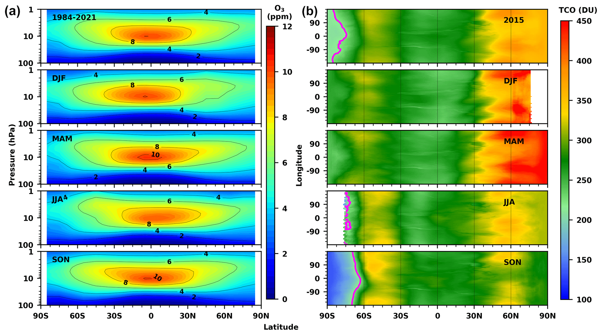
Figure 1 (a) Latitudinal distribution of ozone mixing ratios in ppm averaged for the period 1984–2021 and throughout the seasons, as derived from the GOZCARDS data. (b) The global seasonal and annual distribution of total column ozone (TCO in DU) for 2015 as measured by the Ozone Mapping and Profiler Suite (OMPS) shows the region of the ozone hole (magenta line), i.e. TCO less than 220 DU. The white spaces are data gaps. Here, DJF is December, January and February; MAM is March, April and May; JJA is June, July and August; and SON is September, October and November.

Figure 1b shows the seasonal distribution of TCO across the latitudes for 2015 measured by OMPS. In contrast to mixing ratios, the TCO distribution shows high values in the northern high latitudes in winter and spring and very low values in the SH spring. The Antarctic ozone hole is clearly visible in austral spring, but the analysis for the boreal spring is masked by the data gaps. However, a reduction of 50–60 DU, which is the average TCO loss expected in a normal cold Arctic winter, in 0–50° E and 100–130° E around 70° N, is clearly captured (Goutail et al., 2005). The seasonal variation in ozone in the tropical latitudes is very small, but the SH mid-latitudes show high values in winter, and the Northern Hemisphere (NH) mid-latitudes show high values in spring, as the Brewer–Dobson circulation (BDC) is stronger in winter and spring (Lin and Fu, 2013). Here, we have used the data from OMPS for the year 2015 to show the changes in TCO, since there was a pronounced Antarctic ozone hole in that year.

Figure 2 shows the TCO averaged over the tropics for the period 1978–2022, which is within 250–280 DU in this time period from all available measurements and reanalysis datasets. We also observe a decrease in peak TCO in the tropics during the period 1995–1999 (around 255 DU) when compared to the previous and following years (> 255 DU). However, there is an increase in TCO post-1997, and there is no significant difference (10–15 DU) in TCO among different datasets during the entire period. Furthermore, the bias in measurements from different instruments is within 5–10 DU, which shows that the data are robust and that there is no substantial loss of ozone in the tropics during the period 1979–2022. The tropical column ozone is never below 220 DU. We have also computed the trends in TCO using MERRA-2, ERA5 and satellite data (combined SBUV and OMPS measurements). The satellite-based estimates show significant negative trends (−0.076 ± 0.028 DU yr⁻¹ and −0.093 ± 0.059 DU yr⁻¹) in the pre- and post-1997 periods, whereas the reanalysis data show non-significant trends in both periods. Conversely, the GSG (GOME/SCIAMACHY/GOME2) data yield non-significant positive trends in the post-2000 period.

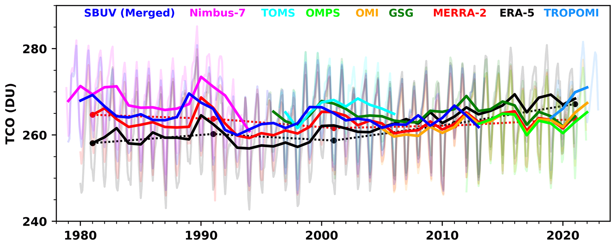
Figure 2 The distribution of total column ozone (TCO in DU) averaged over the tropics (30° S–30° N) from different satellites for the period 1978–2022. The light lines show the monthly distribution, whereas the dark lines show the annually averaged value of TCO. The dotted line shows the decadal distribution of TCO from MERRA-2 and ERA5. The peak in 1991 may be driven by the Mount Pinatubo volcanic eruption.

We have also estimated the trends in ozone in the stratosphere using the SWOOSH (Fig. 3) and GOZCARDS (Fig. S1) data for the period 1984–2022, and the trends are statistically non-significant (at the 95 CI) at most altitudes in both datasets. The SWOOSH estimates for the period 1984–1997 show non-significant but high negative trends of about −0.035 ppm yr⁻¹ in the upper stratosphere and −0.015 ppm yr⁻¹ in the middle and lower stratosphere. Some regions also show non-significant positive trends (0.03–0.04 ppm yr⁻¹) such as the lower stratosphere in all seasons (but DJF and JJA in GOZCARDS, and these are significant). The negative trends indicate the impact of high amounts of stratospheric halogens during the period 1984–1997. In contrast, the estimates for the period 1998–2022 show non-significant positive trends (0.01–0.025 ppm yr⁻¹) throughout the stratosphere across the seasons. The positive trends in other latitudes and altitudes are mostly within 0.01–0.02 ppm yr⁻¹ and are significant. The highest among these trends (0.025 ± 0.01 ppm yr⁻¹) are found in NH and SH low-latitude mid-stratosphere (above 10 hPa) in March, April and May (MAM).

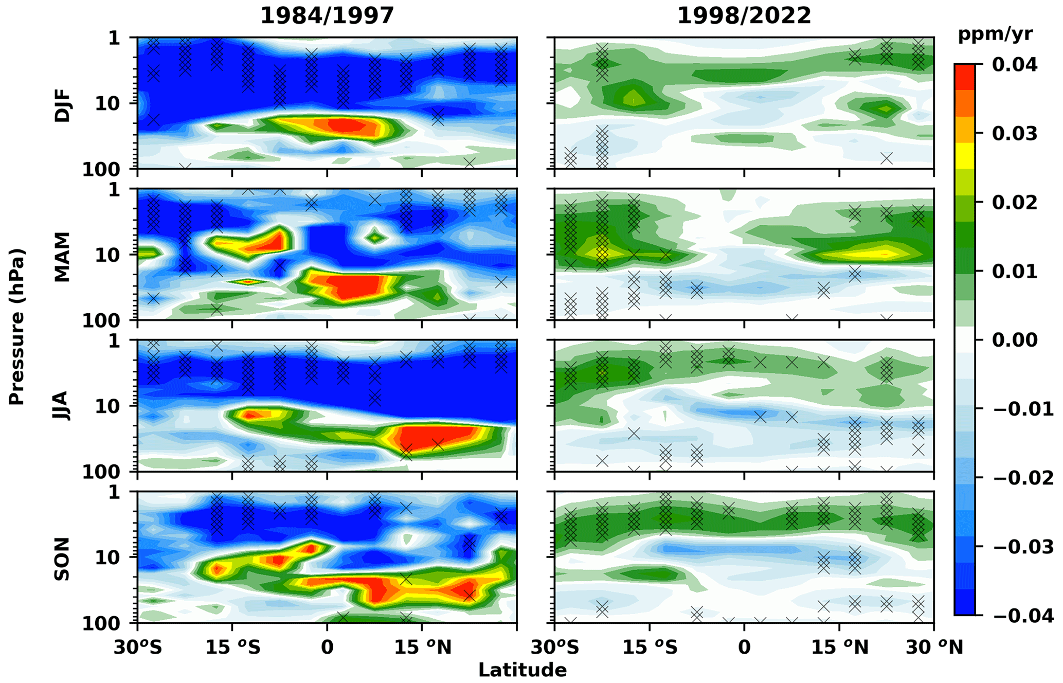
Figure 3 Trends in mixing ratio of ozone estimated for each season using the SWOOSH data for the periods of 1984–1997 and 1998–2022. The stippled regions are statistically significant at the 95 % CI. Here, DJF is December, January and February; MAM is March, April and May; JJA is June, July and August; and SON is September, October and November.

The GOZCARDS data also show similar trends, but those in the upper and middle stratosphere are slightly lower than that in SWOOSH in all seasons, about 0.1–0.2 ppmv yr⁻¹ in 1984–1997. However, the trend in the middle stratosphere in DJF is slightly higher at 15–30° S in GOZCARDS during the pre-1997 period. The trend computed for the post-1997 period is very similar, and those in the lower and middle stratosphere are non-significant in both datasets. Therefore, we have examined the difference between GOZCARDS and SWOOSH ozone, which is shown in Fig. S2. In general, GOZCARDS shows relatively higher values in the middle stratosphere (25–35 km) until 2004, which is the UARS MLS period. However, GOZCARDS shows slightly lower values with SWOOSH during the HALOE period, from 1991 to 2004, within 0.5 ppmv. The agreement between both datasets is excellent in the lower and upper stratosphere and throughout the stratosphere during 2004–2020, within 0.1 ppmv. Our results are consistent with those of Szelag et al. (2020), as they also find significant negative trends in the lower stratosphere (up to −3 % yr⁻¹) but positive trends in the middle and upper stratosphere in spring and summer in the tropics.

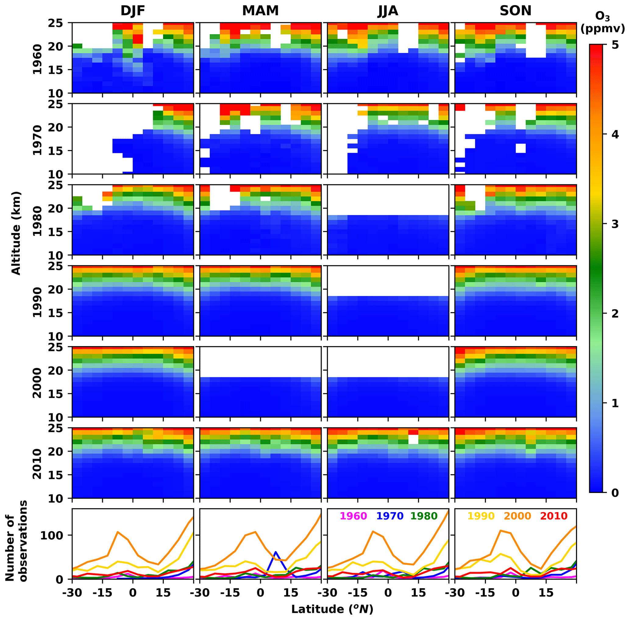
Figure 4 Average of vertical distribution of ozone from the Trajectory-mapped Ozonesonde dataset for Troposphere and Stratosphere (TOST) in each decade from 1960 to 2010. White areas indicate data gaps. Here, DJF is December, January and February; MAM is March, April and May; JJA is June, July and August; and SON is September, October and November. The bottom panel shows the number of ozonesonde observations at 19 km for each decade.

3.2 Tropical ozone variability and trends

Our analyses (Figs. 3, S1, S3 and S5) show that there was substantial ozone loss in the 1984–1997 period at all latitudes and seasons, which is consistent in all the satellite-based (GOZCARDS and SWOOSH) and reanalysis (ERA5 and MERRA-2; see Table S2 in the Supplement) data used in this study. Neutral O₃ trends are also found in the tropics and are consistent in both ozone profile and TCO measurements. Recently, Lu (2022) claimed that there was strong ozone loss that he refers to as an “ozone hole” in the tropics in the past decades (1990–2020), which is reported to be present in all seasons and increasing in size day by day. The author further argues that this “ozone hole” is similar to that in Antarctica and that even the chemical mechanisms causing it were the same. However, there are serious concerns about that particular study and the so-called tropical “ozone hole”. Firstly, the data Lu (2022) used are mainly from the pre-satellite era, and these data have plenty of gaps in the tropical region (Chipperfield et al., 2022). For instance, Fig. 4 shows the data used by Lu (2022), in which there are large data gaps in the tropical latitudes in all 3 decades (1960s, 1970s and 1980s). These data gaps are in the middle stratosphere for 1960 and 1980 but in the entire lower and middle stratosphere for 1970. The ozone values in the tropics are about 20–40 ppbv, and there is hardly any significant change in tropical ozone from 1960 to 2010. Note that there is no signature of an ozone hole in Antarctica in this data (not shown), which also illustrates the problem of TOST data in accurately representing stratospheric ozone. In brief, very small values are observed in TOST in the tropics, and the data gaps make it not suitable for statistical analysis. Secondly, the low-ozone-value region in the tropics is known to the scientific community for long (London and Liu, 1992), and the reason for this is the tropical upwelling branch of BDC that carries air with low ozone to the lower stratosphere (10–20 km).

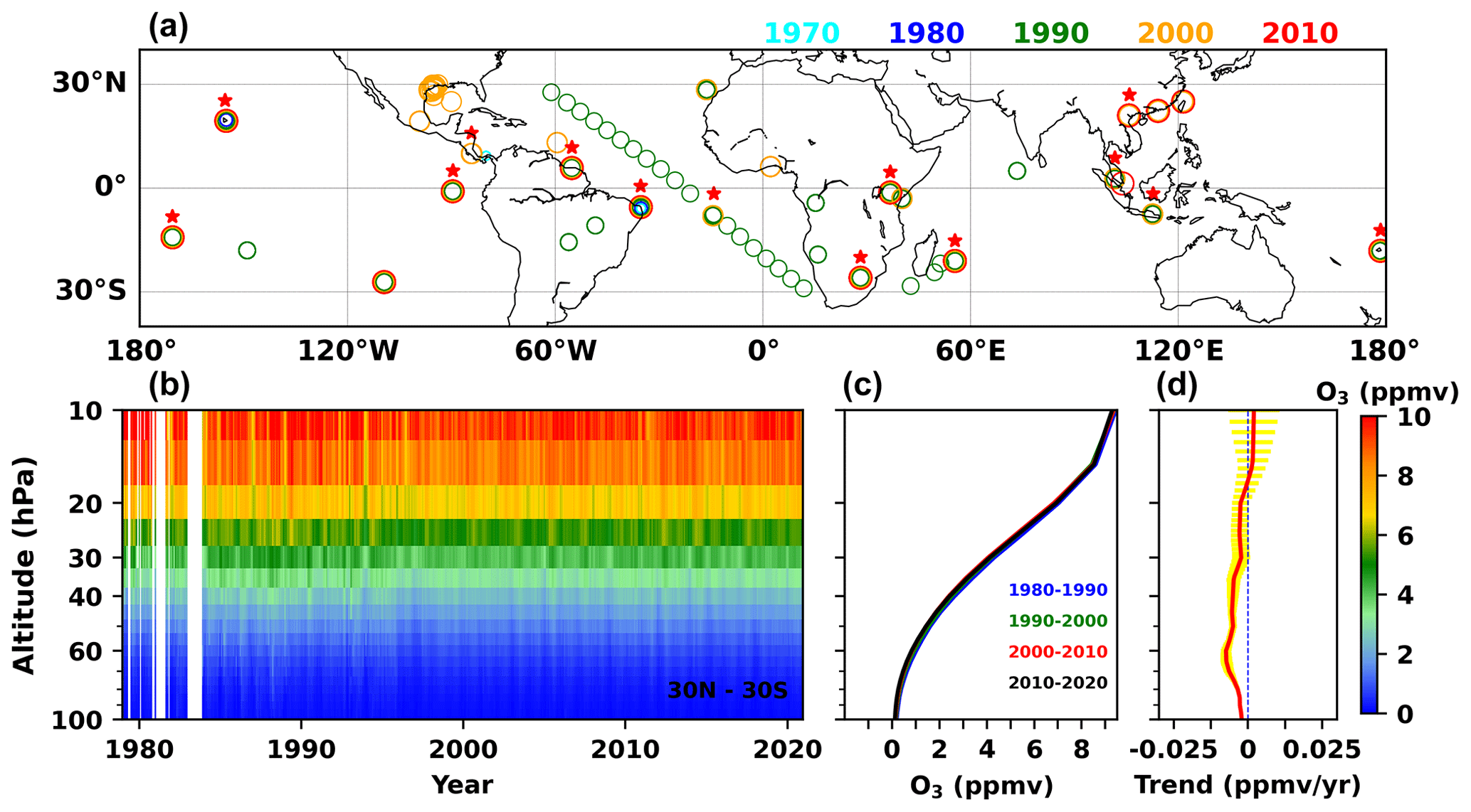
Figure 5 (a) Locations of the ozonesonde stations in the tropics. The Southern Hemisphere ADditional OZonesondes (SHADOZ) stations are marked with a red star. (b) Ozone profiles from WOUDC ozonesonde averaged for the tropics. (c) Mean ozone distribution over each decade in the tropics. (d) The yearly averaged ozone trends for the period 1980–2020.

We have used all ozonesonde measurements available in the tropics from WOUDC to further examine the ozone values (Fig. 5). As expected, very small values are observed in the tropical lower stratosphere, approximately 2 ppm. The decadal change in ozone is also very small (middle panel) in the past 4 decades, and the long-term analysis shows non-significant trends at about 0.01 ± 0.008 ppm yr⁻¹ for all three latitude bands (0–30° N, 0–30° S and 30–30° N/S).

We have also applied the MLR method to find the trend in ozone by using the SWOOSH and GOZCARDS data. The estimated trends are non-significant at most altitudes during the period 1984–1997 (Fig. S7). Both data show a statistically significant decline in ozone in the upper stratosphere (5–1 hPa) during the period 1984–1997. The upper stratosphere shows a negative trend of around −0.035 ppm yr⁻¹, and the middle and lower stratosphere show a negative trend of around −0.015 ppm yr⁻¹. Although much of these tropical regions have noticeable positive trends (0.03–0.04 ppm yr⁻¹), they are non-significant. However, the trend estimated for the period 1998–2022 suggests that ozone is increasing (0.025–0.05 ppm yr⁻¹) in the stratosphere across the seasons (Figs. S8 and S9), except in the lower-latitude lower stratosphere where the values are slightly negative (−0.01 ± 0.002 ppm yr⁻¹) and are statistically significant.

Furthermore, we have collated the SHADOZ measurements to the nearest grids of TOST data and estimated the linear trends and bias of TOST at 15–35 km. The decadal mean of SHADOZ data does not show any significant change in ozone concentrations, except above 30–32 km, which can also be due to balloon measurement errors at these altitudes (Fig. S10). The trend estimated for the individual SHAODOZ stations exhibits either significant positive trends of about 0.01 ± 0.005 ppmv yr⁻¹ or significant negative trends of about 0.01–0.035 ppm yr⁻¹ in the lower stratosphere (below 25 km). The middle stratospheric trends are neutral or positive at the SH stations.

The bias in TOST data, which were used by Lu (2022) and estimated using the collated SHADOZ measurements in the tropics, is shown in Fig. 6. The TOST data show hardly any bias below 20 km at most stations but show a low bias (1–1.5 ppmv) above that at all stations, except Nairobi, Hilo and Irena, where the TOST data show higher bias of about 1–1.5 ppmv. This is one of the reasons for the low ozone found in the study by Lu (2022). In addition, the comparison between TOST and satellite data (GOZCARDS and SWOOSH) shows that TOST is biased low by 0.1–0.45 ppmv in the lower stratosphere, which increases with altitude (Fig. S11). Also, the air transported vertically from the tropical tropopause to the stratosphere is usually characterized by very low ozone values. Therefore, the low tropical ozone values are driven by dynamics (Telford et al., 2009; Chipperfield et al., 2018).

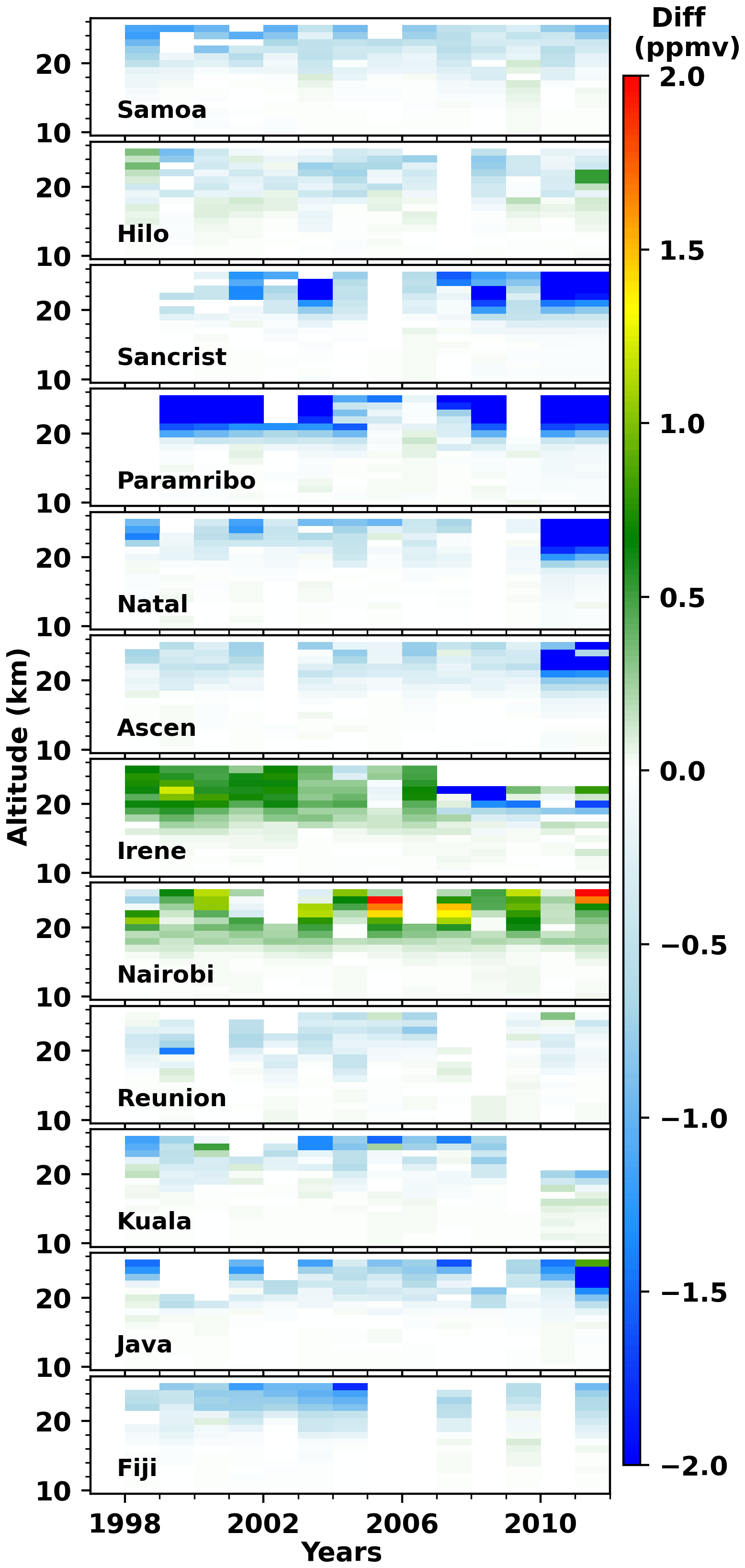
Figure 6 The bias in TOST data (TOST–SHADOZ in ppmv) calculated using collated measurements from SHADOZ measurements for the period 1998–2012.

Thirdly, Lu (2022) used the percentage change in ozone to define the “ozone hole”, which is not a good metric to show how much ozone is present in a region. Rather, an ozone hole definition (i.e. ozone values below 220 DU) should be based on the amount of ozone present in a region, not relative to some other decade or a period. Apart from that, ozone loss is a seasonal process in the polar regions; therefore the comparison must be made with respect to the period of ozone loss with respect to its starting year. In addition, the impact of the “ozone hole” depends on the amount of ozone present, not the amount relative to previous decades in that region. Fourthly, the amount of TCO in the tropical region was never below 220 DU, and there is a slight increase in ozone in the stratosphere and troposphere after the year 2005 (see Fig. 2). Additionally, Lu (2022) incorrectly assigns tropical altitudes above 10 km to the stratosphere, but the troposphere extends up to 16–18 km there (Seidel et al., 2001), in which very low ozone can be found over the tropical Pacific due to vertical transport of clean boundary layer air by convection (Kley, 1997). Lu (2022) therefore incorrectly claims that Polvani et al. (2017) and Newton et al. (2018) reported very low ozone values in the tropical lower stratosphere. Polvani et al. (2017) only discuss ozone at 70 hPa (18 km) and higher, whereas Newton et al. (2018) attribute the low ozone to “uplift of almost-unmixed boundary-layer air” to altitudes of 100–150 hPa (14–17 km). Therefore, no TCO measurements show values below 220 DU, but all depict a small increase in ozone after 2005, in contrast to the claim made by Lu (2022). Fifthly, the formation of polar vortices and PSCs are key to ozone loss in the polar winter and spring. Formation of PSC particles is also required for the cosmic-ray-driven electron-induced reaction (CRE) mechanism put forward by Lu (2022). However, no such phenomena are reported for the tropical stratosphere; indeed, there is no evidence for ice particles in the tropical stratosphere in measurements (Zou et al., 2022; Chipperfield et al., 2022). Therefore, no such heterogeneous ozone loss is observed in the low latitudes, and there is no basis for the CRE theory (Grooß and Müller, 2011). Finally, it was already well-established a couple of decades ago based on all then available measurements that the trends in tropical stratospheric ozone are largely absent or minimal at best for the period 1979–1997 (Staehelin et al., 2001), which is neither acknowledged nor discussed in Lu (2022).

3.3 Reasons for the lower values of ozone in the tropics

We also replicated the analysis made by Lu (2022), in addition to a detailed analysis by Chipperfield et al. (2022) with the same TOST data, and find the following issues with Lu's claim on tropical ozone loss. (i) The TOST data Lu (2022) used are sparse in the tropical latitudes in the troposphere and stratosphere in all 3 previous decades of the 1960s, 1970s and 1980s (see Fig. 4, top three panels, and Fig. S12). Although the values are very small (20–30 ppb), which is expected there, the data cannot be subtracted from other datasets with gaps in them. One cannot claim any scientific process with interpolated data with huge gaps, as shown here. (ii) As opposed to Lu's statement of continuous decline, we find a slight increase or no significant change in ozone from 1980 to the next decades in various independent datasets.

The tropical stratospheric ozone has increased by at least 10–20 ppb in the past decades according to our analysis of a wide range of available data, in contrast to Lu's claim that the so-called tropical “ozone hole” was expanding. The recent strengthening of the BDC has reduced the ozone values in the tropical stratosphere, which is reflected in the analysis of ozone for recent decades (Butchart et al., 2006). Due to the accelerated motion of air in the tropics, the time for photochemical production of ozone is reduced, which is another reason for the declining trend in ozone there (Avallone and Prather, 1996). The enhanced ozone transport to the middle latitudes further reduces ozone in the lower stratosphere (Wargan et al., 2018). In addition to the changes in relative strength of upper and lower branches of the BDC (Butchart et al., 2006; Keeble et al., 2018; Abalos et al., 2019), the increase in halogen-containing short-lived species as there are no regulations or polices to curb them (Hossaini et al., 2015; Villamayor et al., 2023), widening of extratropical troposphere (Zubov et al., 2013; Bognar et al., 2022), increased aerosol loading (Andersson et al., 2015), and unexpected emissions of CFC-11 (Fleming et al., 2020) and inorganic iodine (Cuevas et al., 2018; Karagodin-Doyennel et al., 2021) could also decrease tropical lower-stratospheric ozone. There is also a study suggesting that the reduction in solar activity might reduce ozone in the tropical regions (Arsenovic et al., 2018). However, trend detection in the tropical latitudes is difficult due to the large dynamical variability there, as also found by Stone et al. (2018). Note that the warming of the tropical upper troposphere causes a sharp temperature gradient between the tropics and mid-latitudes, which would push the jet and thus lift the tropopause. This, in turn, produces enhanced meridional transport between the regions (tropics to mid-latitudes) through the lower branch of BDC and is projected to continue through the turn of the century. Henceforth, tropical lower-stratospheric ozone is also expected to decline further in the coming decades (Zubov et al., 2013). In brief, the change in tropical ozone presented in Lu (2022) is mostly due to the issues in the data used in his study, and the lower values of ozone in the troposphere are driven by dynamics. In the tropics, there are no new ozone loss processes, and there is certainly no “ozone hole” formed, as claimed.

Apart from these arguments, the claim by Lu (2022) regarding the lower ozone values and their impact is based on the volume (molar) mixing ratios in the tropical lower stratosphere. However, the ozone peak is around 30–35 km at these latitudes when we consider volume mixing ratios (molar mixing ratios); hence, the analyses of Lu (2022) miss the major part of tropical ozone. When we examine the column values, they are never below 220 DU, and there is no big threat from UV radiation.

4 Conclusions

The analyses of stratospheric ozone in the tropics presented here show a consistent picture of ozone evolution in the past 4 decades. There is no significant loss or increase in tropical stratospheric ozone, although slightly negative trends are found during the period of 2000–2020. Recent studies have suggested that the negative trends in the tropical upwelling region are caused by dynamical processes, including the increase in the speed of BDC. This is clearly pictured in the time series of tropical ozone in recent years. The long-term trend in tropical TCO for the period 1998–2022 also shows no notable difference from the past decades. The claim of Lu (2022) is solely based on one decadal dataset, which has only a few profiles (see Fig. S12), and the dataset is available only for the lower stratosphere. On the other hand, we have analysed a set of satellite, balloon-borne, ground-based and reanalyses data here to examine tropical ozone, and we find that the claims are not properly based on measurements or model simulations and that the data Lu (2022) used are inadequate to analyse tropical stratospheric ozone. In addition, there is no such threat as Lu (2022) claimed due to the slightly negative trends in ozone in the past 2 decades (1998–2022), as these changes are driven by stratospheric dynamics. In summary, there is no tropical “ozone hole”, and the evidence provided by Lu (2022) for such a phenomenon is seriously flawed.