Impact of weather patterns and meteorological factors on PM_2.5 and O₃ responses to the COVID-19 lockdown in China

Haze events in the North China Plain (NCP) and a decline in ozone levels in Southern Coast China (SC) from 21 January to 9 February 2020 during the COVID-19 lockdown have attracted public curiosity and scholarly attention. Most previous studies focused on the impact of atmospheric chemistry processes associated with anomalous weather elements in these cases, but fewer studies quantified the impact of various weather elements within the context of a specific weather pattern. To identify the weather patterns responsible for inducing this unexpected situation and to further quantify the importance of different meteorological factors during the haze event, two approaches are employed. These approaches implemented the comparisons of observations in 2020 with climatology averaged over the years 2015–2019 with a novel structural SOM (self-organising map) model and with the prediction of the “business as usual” (hereafter referred to as BAU) emission strength by the GBM (gradient-boosting machine) model, respectively. The results reveal that the unexpected PM_2.5 pollution and O₃ decline from the climatology in NCP and SC could be effectively explained by the presence of a double-centre high-pressure system across China. Moreover, the GBM results provided a quantitative assessment of the importance of each meteorological factor in driving the predictions of PM_2.5 and O₃ under the specific weather system. These results indicate that temperature played the most crucial role in the haze event in NCP, as well as in the O₃ change in SC. This valuable information will ultimately contribute to our ability to predict air pollution under future emission scenarios and changing weather patterns that may be influenced by climate change.

1 Introduction

The coronavirus disease 2019 (COVID-19) pandemic has lasted for 4.5 years and has led to over 7 million​​​​​​​ deaths globally as of June 2023 (WHO, 2024). The Chinese government implemented strict lockdown measures nationwide during the first 2 months of 2020 to curb the spread of this pandemic (Le et al., 2020), which led to significant reductions in anthropogenic emissions, especially in the transportation sector (Xu et al., 2020; Wang et al., 2021; Liu et al., 2021). As a result, a decline not only in NO₂ but also in PM_2.5, PM₁₀, SO₂, and CO concentrations on a national scale was indicated by both satellite and ground-based measurements, although with the negative consequence of enhancements in O₃ concentrations (Shen et al., 2022; Liu et al., 2021; He et al., 2020). Contrary to the situation in other regions from 21 January to 9 February 2020, Northern China (NC) and Southwestern China (SWC) experienced severe haze pollution and decreased O₃ situations, respectively (Le et al., 2020; Huang et al., 2021; Wang et al., 2020). This exceptional situation during the haze event in China thus lends itself to a large-scale “experiment” to study the unusual phenomenon driven by atmospheric chemistry and meteorology.

PM_2.5 and ground-level ozone (O₃), especially in highly polluted regions, adversely affect human health (Lelieveld et al., 2015), agriculture (Feng et al., 2015; Wang et al., 2007), and the Earth's radiation budget (Liao et al., 2015; Dang and Liao, 2019), thereby leading to premature mortality, decreases in crop yields, and altering the climate. Anthropogenic PM_2.5, in addition to being generated by fossil fuels and biomass burning, is also produced through the reactions of inorganics (e.g. NO, NO₂, SO₂, and NH₃) and volatile organic compounds (VOCs) (Zheng et al., 2017). In contrast, O₃ is not directly emitted but is formed through a series of photochemical reactions involving multiple precursors (e.g. carbon monoxide (CO), methane (CH₄), VOCs, NO, and NO₂) (Ge et al., 2013). Apart from intense local primary emissions and secondary chemical formation, stagnant meteorological conditions and regional transport are two additional contributors to severe haze and O₃ pollution events (Shen et al., 2020). Recently, a series of air quality regulations (Clean Air Plans, CAPs) released by the Chinese government have resulted in a notable decrease in anthropogenic emissions, leading to a substantial improvement in air quality due to reductions in PM_2.5 concentrations but a nationwide enhancement of O₃ pollution in China (Shen et al., 2020; K. Li et al., 2019). It is known that the impacts of meteorological conditions and atmospheric chemical processes could result in non-linear responses of PM_2.5 and O₃ to the decreases in their precursor concentrations (H. Li et al., 2019; Li et al., 2020). However, the specific responses of air pollutants and atmospheric chemistry to emissions and meteorological conditions have not been clearly determined.

For the haze event in China introduced above, recent studies on the topic suggested that complex atmospheric chemistry processes triggered by emission reductions and meteorological conditions are responsible for the unexpected haze formation regionally during the COVID-19 lockdown (Le et al., 2020; Fu et al., 2021). In detail, the substantial decrease in NO₂ emissions during the COVID-19 lockdown resulted in an increase in O₃ levels and nighttime NO₃ radical formation, enhancing the atmospheric oxidation capacity (AOC) and facilitating the formation of secondary aerosols. Additionally, the presence of anomalous relative humidity promoted heterogeneous chemistry processes (Le et al., 2020; Huang et al., 2021; Ma et al., 2022). After the formation, more generated secondary aerosols were transported toward the in situ measurement station in northern China (Lv et al., 2020). Meanwhile, some research pointed out that the high ambient humidity is also the key to the NC haze from the perspective of adjusting pH to control the formation efficiency of nitrate aerosol, which is one of the major species for NC haze (Chang et al., 2020; Sun et al., 2020). In addition to the influence of changes in chemical reactions, a physical mechanism known as the aerosol–planetary boundary layer (PBL) interaction is also considered to have had a significant impact on the haze formation (Su et al., 2020). For O₃, the decline in climatology in SC was attributable to the weakened photochemistry reactions due to the emission reductions in and the dilution effect of the clean air masses on the mass loadings of NO_x and VOC (Fu et al., 2021; Liu et al., 2021). Overall, meteorological conditions always played a critical role; high relative humidity is the trigger of aerosol heterogeneous chemistry by adjusting the particle pH or providing a reaction medium. Meanwhile, the transport of the secondary aerosol or clean air masses and shallow PBL height are primarily driven by wind and pressure, respectively. Importantly, the above weather elements are modulated synergistically by synoptic-scale weather patterns (SWPs) or large-scale atmospheric circulations.

Numerous studies have been conducted worldwide to explore the direct connections between SWPs and air quality fields (Dayan and Levy, 2002; Demuzere et al., 2009; Pope et al., 2015; Hegarty et al., 2007; Bei et al., 2016; Jiang et al., 2017), indicating that good air quality conditions are often observed under cyclonic weather systems with certain types and positions, while poor air quality is frequently associated with anticyclonic conditions. However, the relationship between air quality and SWPs can differ depending on location, time, and pollutants (Jiang et al., 2017; Liao et al., 2017). The classification methods for SWPs employed in these studies can generally be categorised into the following three groups: subjective (manual), mixed (hybrid), and objective (automated) (Huth et al., 2008). Objective classification methods for SWPs are known for their speed, objectivity, and high reproducibility, often achieving classification 100 % automatically. On the other hand, manual approaches for SWPs have the advantage of allowing the user to control the selection of representative weather types (Lewis and Keim, 2015). Hybrid classification combines the strengths of both manual and automated techniques, where the users define the classification types, but the classification process itself is performed automatically (Frakes and Yarnal, 1997; Lewis and Keim, 2015; Huth et al., 2008). At present, the subjective method was used to investigate the contribution of six SWPs to PM_2.5 pollution in Northwest China (Bei et al., 2016). While subjective approaches are suitable for analysing short time series, they have significant limitations when applied to large datasets spanning extended periods of time (Chen et al., 2022). Hybrid classification for SWPs is more popular than the subjective one and was applied to explore the impact of SWPs on O₃, PM_2.5 and CO in the North China Plain (NCP), Yangtze River Delta (YRD), and Eastern China, respectively (Zhang et al., 2013, 2016; Han et al., 2018; Liao et al., 2017). As an objective classification and with its advantages, the self-organising map (SOM) algorithm has been used to identify the impact of different SWPs on O₃ and PM_2.5 in the YRD and Sichuan Basin (SCB), respectively (Shu et al., 2020; Zhan et al., 2019). In addition, the principle component analysis T mode, k-means clustering, and other clustering approaches (like the Lamb–Jenkinson method) also were adopted to quantify the impact of SWPs on O₃ in NCP (Miao et al., 2017; Dong et al., 2020; Liu et al., 2019).

Based on the studies mentioned above, previous research on the drivers for unusual haze and O₃ decline events has concentrated on the influence of atmospheric chemistry processes accompanied by the anomaly of one or two weather elements but has not yet focused on the impact of weather elements in a comprehensive and synergistic way. Therefore, we here investigate the effect of anomalies in weather conditions with respect to climatology on PM_2.5 and O₃ concentrations during the haze event in the COVID-19 lockdown, specifically. To this end, we apply a novel SOM algorithm called structural SOM (S-SOM) to identify the most meaningful clustering number of weather patterns and compare it to other traditional SOM methods including ED-SOM and the SOM algorithm based on the Pearson correlation coefficient (hereafter named COR-SOM). Furthermore, after determining the weather patterns, we evaluate the contribution of SWPs to PM_2.5 and O₃ changes during the COVID-19 lockdown in China. Last, to better understand what role each meteorological factor played in the PM_2.5 and O₃ pollution during this period, the SHapley Additive exPlanation (SHAP) approach is used to evaluate their relative importance for the predictions of the machine learning (ML) model. The knowledge gained will ultimately help to predict air pollution under future emission scenarios and weather patterns potentially altered by climate change.

2 Method

2.1 Observational and model dataset sources

The hourly observation dataset during the first 2 months (January and February) from 2015 to 2020, including two air pollutants (PM_2.5 and O₃) and six meteorological factors (pressure is P, precipitation is Precip, temperature is Temp, relative humidity is RH, wind speed is WS, wind direction is WD), was divided into two parts, namely the training dataset and test dataset, which were used to build a prediction model based on machine learning. Air pollutant and meteorological station datasets were downloaded from the National Environmental Monitoring Centre (http://www.cnemc.cn, last access: 28 May 2024) and the National Meteorological Science Data Center repository (https://data.cma.cn, last access: 28 May 2024). To better understand the climatological behaviour of air pollutants, 367 surface measurement stations across China are divided into eight different regions (including NCP for North China Plain, IM for Inner Mongolia, NEC for North Eastern China, YRD for Yangtze River Delta, CS for Central South, SC for Southern Coast, TP for Tibet Plateau, and NWC for North Western China) based on different typical climate characteristics (see the climate classification scheme at https://www.resdc.cn/data.aspx?DATAID=243, last access: 28 May 2024; Fig. 1). In addition, hourly surface ERA5 data with 0.25 × 0.25 spatial resolution, including mean sea level pressure (MSLP) (at 14:00 local time per day) and total solar radiation (SR), were retrieved from the European Centre for Medium-Range Weather Forecasts (ECMWF).

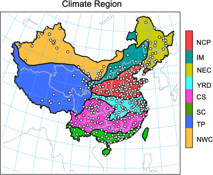
Figure 1 The spatial distribution of air quality measurement stations in different climate regions (circles represent surface measurement stations; colours indicate different climate zones). The abbreviations used in the figure are as follows: NCP – North China Plain; IM – Inner Mongolia; NEC – North Eastern China; YRD – Yangtze River Delta; CS – Central South; SC – Southern Coast; TP – Tibet Plateau; and NWC – North Western China.

2.2 Structural SOM algorithm (S-SOM)

The SOM algorithm involves an iterative learning processes that progressively update the nodes in the output map until they converge to a stable solution. During each learning step, the SOM algorithm selects an input vector in a random way and then searches for a node that best matches that particular vector. Traditionally, the Euclidean distance (ED) in the SOM algorithm is often used as a criterion to search for the winning node that is closest to an input vector. ED is very popular in the SOM algorithm but with significant shortcomings when applied to compare structured inputs with temporal or spatial orders. As a result, the limitations of ED become particularly significant in climatology research, where the data are often given with a spatial and temporal structure, which might result in the degradation of the spatial correlations between air pressure patterns in weather maps (Doan et al., 2021).

The S-SOM algorithm is executed following the procedure proposed by Kohonen (1982) and is widely used in many studies. To begin, an S-SOM is initialised by configuring the SOM node and determining the number of training iterations. The training process involves three key steps:

1. selecting an input vector,

2. identifying the best-matching unit in the SOM for the input vector, and

3. updating the weight vectors of the SOM nodes using specific parameters.

The only difference between the traditional SOM and S-SOM is that the similarity index (S-SIM) rather than ED is used to compare the similarity between vectors. S-SOM was first proposed by Wang et al. (2004) and can be expressed in the following equation:

$$\begin{array}{}\text{(1)}& \text{S-SOM}(\mathit{x},\mathit{y})=\left[l(\mathit{x},\mathit{y}{)}^{\mathit{\alpha }}\times c(\mathit{x},\mathit{y}{)}^{\mathit{\beta }}\times s(\mathit{x},\mathit{y}{)}^{\mathit{\gamma }}\right].\end{array}$$

Here, x and y are two vectors, and l, c, and s are three comparison measurements representing luminance, contrast, and structure, respectively. The three comparison functions are as follows:

$$\begin{array}{}\text{(2)}& {\displaystyle }l(\mathit{x},\mathit{y})={\displaystyle \frac{\mathrm{2}{\mathit{\mu }}_x{\mathit{\mu }}_y+c_{\mathrm{1}}}{{\mathit{\mu }}_x^{\mathrm{2}}+{\mathit{\mu }}_y^{\mathrm{2}}+c_{\mathrm{1}}}},\text{(3)}& {\displaystyle }c(\mathit{x},\mathit{y})={\displaystyle \frac{\mathrm{2}{\mathit{\sigma }}_x{\mathit{\sigma }}_y+c_{\mathrm{2}}}{{\mathit{\sigma }}_x^{\mathrm{2}}+{\mathit{\sigma }}_y^{\mathrm{2}}+c_{\mathrm{2}}}},\text{(4)}& {\displaystyle }s(\mathit{x},\mathit{y})={\displaystyle \frac{{\mathit{\sigma }}_{xy}+c_{\mathrm{3}}}{{\mathit{\sigma }}_x{\mathit{\sigma }}_y+c_{\mathrm{3}}}}.\end{array}$$

Here, the average and standard deviation values are represented by μ and σ, respectively. The parameters c₁, c₂, and c₃ are used to stabilise the division operations involving a weak denominator. The luminance, contrast, and structure in the S-SOM formula are three elements of human perception. Luminance assesses the similarity in brightness values between images. Contrast quantifies the similarity in illumination variability among images. Last, the structure measures the correlation in spatial interdependencies between images, reflecting how the spatial elements of the images are related to each other (Wang and Bovik, 2009). Here, we can set the values of c₁, c₂, and c₃ to 0 and the weights α, β, and γ to 1 to simplify the model (Doan et al., 2021). The final expression shows

$$\begin{array}{}\text{(5)}& \text{S-SOM}(\mathit{x},\mathit{y})={\displaystyle \frac{\left(\mathrm{2}{\mathit{\mu }}_x{\mathit{\mu }}_y\right)\left({\mathit{\sigma }}_{xy}\right)}{\left({\mathit{\mu }}_x^{\mathrm{2}}+{\mathit{\mu }}_y^{\mathrm{2}}\right)\left({\mathit{\sigma }}_x^{\mathrm{2}}+{\mathit{\sigma }}_y^{\mathrm{2}}\right)}}.\end{array}$$

As the function shows, S-SOM ranges from −1 to 1. A value of 1 indicates complete similarity, while a value of −1 indicates complete dissimilarity. S-SOM offers robust, user-friendly, and comprehensible alternatives to the conventional ED approach, particularly when dealing with datasets with a spatial and temporal order (Wang and Bovik, 2009).

2.3 Gradient-boosting machine (GBM) model

The impact of meteorological factors on the variation in the air pollutant concentrations is typically determined via chemical transport models. However, these model predictions are associated with substantial uncertainty, since they rely on the correct quantification of changes in the emission inventory of each city under multi-faceted anthropogenic air pollution interventions (e.g. clean-air plans and COVID-19 lockdown measures). Besides, uncertainties can also be derived from the chemical mechanism (Knote et al., 2015; Weng et al., 2023). Here, a gradient-boosting machine (GBM) model was trained with observations of meteorological factors, with the GBM being able to capture the location-specific characteristics and thus being suitable for the prediction of air pollutant concentrations attributable to the impact of meteorology in different cities across China. Observations of meteorological factors, together with time variables from 2015 to 2019, are considered to be the training dataset to predict the concentrations of PM_2.5 and O₃ in China. The meteorological factors are listed as follows: P, Precip, Temp, RH, WS, and WD. The time variables include the Julian day (JD), day of week (DOW), holidays, and Chinese New Year (CNY) days in each year. For the GBM prediction model, cross-validation is mainly used to estimate how accurately a predictive model will perform in practice. To check the accuracy of the ML model used in our study, a time series split rolling cross-validation based on five splits was used, for which data used for the training task always preceded the data used for validation. In detail, the ML training model was used for 2015, 2015–2016, 2015–2017, 2015–2018, and 2015–2019, while the testing of the model then was implemented over the first 2 months of 2016, 2017, 2018, 2019, and 2020, respectively (Shen et al., 2022). The hyperparameters of the model that we selected are as follows: “number_leaves”, “objective”, “min_data_in_leaf”, “learning_rate”, “feature_fraction”, “bagging_fraction”, “bagging_freq”, and “metric” (detailed parameter information of the model can be accessed from https://lightgbm.readthedocs.io/en/latest/Parameters.html, last access: 28 May 2024). After selecting the best ML model under cross-validation, a ML experiment was designed to make a prediction of PM_2.5 and O₃ in the first 2 months of 2020.

2.4 SHapley Additive exPlanation (SHAP) method

Quantifying the importance of input features of the GBM model is as vital as the overall accuracy of the prediction itself. However, interpreting the higher accuracy achieved by ensemble or ML models on certain datasets can be a challenging task. To deal with this contradiction between higher accuracy and non-interpretability, SHAP, a game theory approach, is applied to calculate the importance value for each specific independent feature. In brief, the SHAP value of each feature is attributed to the difference in one prediction output with one feature versus the prediction output without this corresponding feature. SHAP's local explanations can vary in terms of being positive or negative, reflecting how predictors influence the predicted outcome. In contrast, other ML methods typically yield a single positive value, indicating overall importance. Specifically, in local interpretability analysis (Lundberg et al., 2020), SHAP indicates the contribution of each variable to the prediction of a specific sample. This contribution is assessed from the base value (the predicted mean value) to the final model output. Variables that push the prediction to higher values are displayed as positive, while those decreasing the prediction are shown to be negative. For each predicted model with n variables in one sample (x_l) and the predicted output f(x_l), the equation of the prediction function is described as follows:

$$\begin{array}{}\text{(6)}& f\left(x_l\right)=E_{\mathrm{0}}(f,x)+\sum _{m=\mathrm{1}}^n{E}_m\left(f,x_l\right),\end{array}$$

where x_l is the input with variable m in the prediction model f generating the SHAP value of E_m(f,x_l). E₀(f,x) is the expected value for the prediction model over the whole dataset.

3 Results

3.1 Spatial variations in the air pollutant and meteorology in climatology

The spatial distribution of the fractional differences in air pollutant concentrations during the haze event from 21 January to 9 February 2020, calculated between mean values during the event in 2020 and the values averaged over the same period from 2015 to 2019, for all six air pollutants is shown in Fig. 2. Half of the climate regions, including the YRD, CS, SC, and TP, showed different magnitudes in the decreases (increases) (Table 1) in the climatology for PM_2.5, PM₁₀, NO₂, SO₂, and CO (O₃), which were primarily attributed to the significant anthropogenic emission reduction during the COVID-19 lockdown (Nie et al., 2021; Wang et al., 2022; Shen et al., 2022). However, contrary to expectations, PM_2.5 concentrations did not drop as anticipated at the beginning of the lockdown in NCP, IM, NEC, and NWC. Instead, these regions experienced an unexpected increase of 8.6 %, 31.8 %, 22.3 %, and 2 % compared to climatology during the same period, respectively. Even though the decline was small, O₃ showed an unexpected drop of −0.8 % in SC when compared to climatology during the same period. Our recent work also found a −0.9 % decline in O₃ driven by the meteorological effect during the COVID-19 lockdown across China (Shen et al., 2022). As a fractional difference compared to climatology, the spatial distribution of the key meteorological variables RH, P, Precip, Temp, and WS are shown in Fig. 3. Generally, positive RH and negative WS anomalies are always accompanied by the strong regional elevation of PM_2.5 in NCP, NEC, IM, and NWC. Positive P anomalies coupled with increased PM_2.5 demonstrate the most prominent regional characteristics in NEC. In SC, the most noticeable features were observed as a combination of hotspot Precip anomalies and decreased O₃ levels. Overall, the regional characteristics of PM_2.5 and O₃ all have a close relationship with different meteorological anomalies, which are usually controlled by the regionally prevailing SWPs.

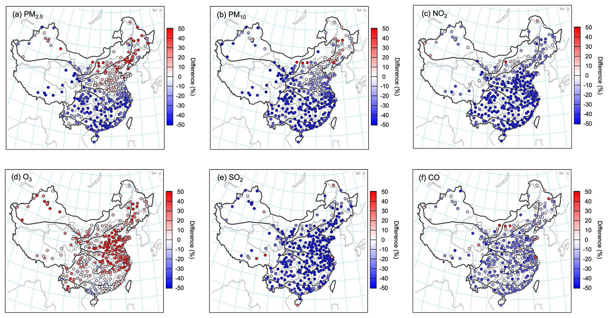
Figure 2 The spatial distributions of fractional differences between mean values during the haze event in 2020 and the climatology over the same period during the years 2015–2019 for six air pollutants (including PM_2.5, PM₁₀, NO₂, O₃, SO₂, and CO).

Table 1 The climate zones and mean fractional climatology anomalies (2020 – mean (2015–2019)) of six air pollutants across China.

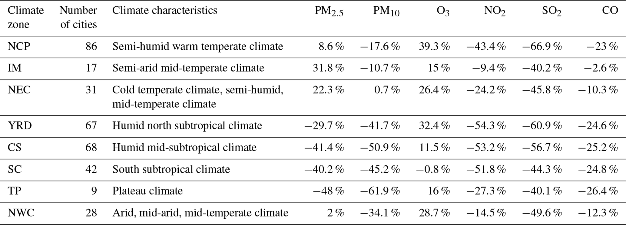
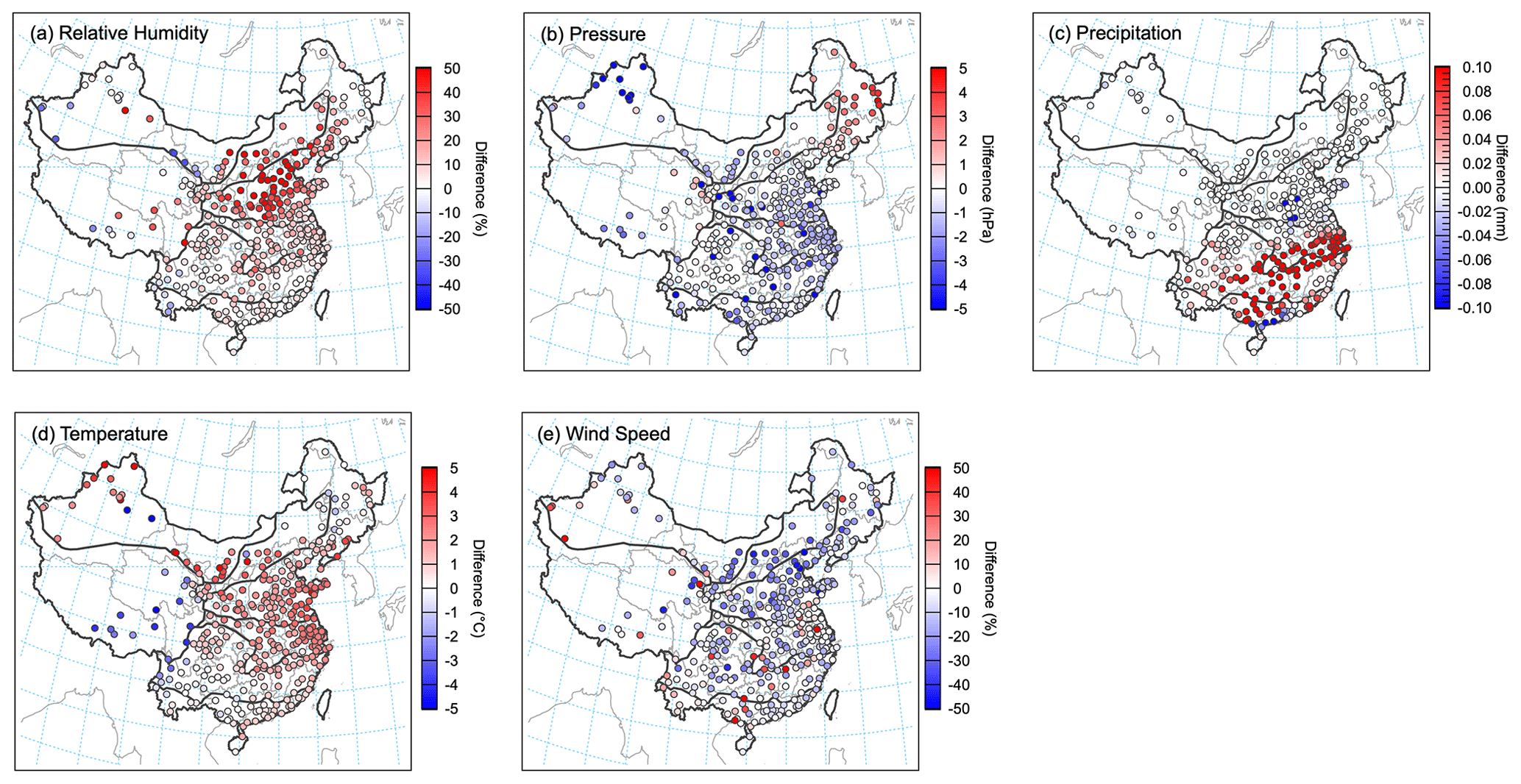
Figure 3 The spatial distributions of differences between mean values during the haze event in 2020 and the climatology over the same period of the years 2015–2019 for meteorological factors (including relative humidity, pressure, precipitation, temperature, and wind speed).

3.2 Identification of the SWPs during the unexpected haze event

To identify which SWPs can regionally induce an unexpected PM_2.5 increase and O₃ reduction compared to climatology averaged over the years 2015–2019, three different SOM methods were employed to identify different types of SWPs (from two to eight) using MSLP data in the first 2 months from 2015 to 2020 over China. Figure 4 shows MSLP patterns identified by S-SOM, COR-SOM, and ED-SOM running three nodes, respectively. Taking this three-node analysis as an example, we find that the three SWPs identified by S-SOM (Fig. 4a, b, and c) are clearly distinct from each other. On the other hand, ED-SOM (Fig. 4d and e) and COR-SOM (Fig. 4g and h) both classify two similar SWPs characterised by high-pressure systems over Siberia, thus resulting in a failure of clustering. This interpretation is supported by the result of clustering the number distributions for the three-node SWPs (Fig. 5d). It should be noted that cluster numbers do not necessarily correspond to the same pattern between S-, ED-, or COR-SOM. Here, it is found that S-SOM results are in a more “ordered” clustering of nodes, where a prominent node (62.9 %) is accompanied by two non-dominant nodes (7.5 % and 29.5 %). On the other hand, both ED-SOM and COR-SOM exhibit relatively similar cluster sizes with percentages of 27 %, 35.1 %, and 37.9 % for ED-SOM and 40.7 %, 34.6 %, and 24.7 % for COR-SOM, highlighting the prevalence of a more “flat” clustering pattern. It can be concluded that the better classification method for three-node SWPs is S-SOM with an ordered clustering number distribution accompanied by a prominent node (Doan et al., 2021). This consistent finding is also observed in other cases (e.g. node numbers smaller or greater than 3; Figs. S1–S12 in the Supplement). Then, we make a further comparison of the node number distribution of S-SOM (Fig. 5a), ED-SOM (Fig. 5b), and COR-SOM (Fig. 5c) in each year and find that S-SOM always has a prominent node with a value of more than 50 % (2015 with 50 %, 2016 with 85 %, 2017 with 64 %, 2018 with 81 %, 2019 with 63 %, and 2020 with 55 %), and the cluster sizes for ED-SOM and COR-SOM are close to each other as well, which is consistent with a recent study indicating a better performance of S-SOM (Doan et al., 2021). Therefore, in addition to the algorithmic advantages, the characteristics of ordered clustering nodes reinforce the superiority of the S-SOM approach.

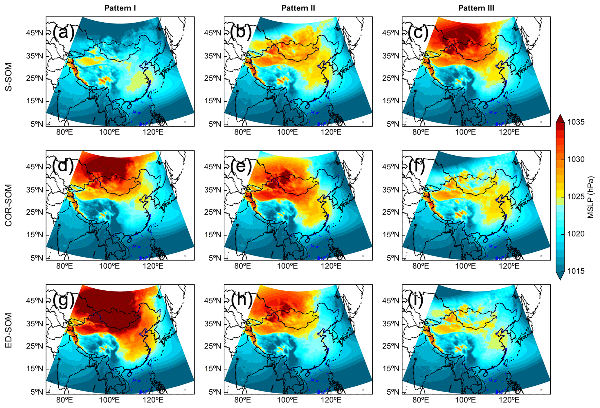
Figure 4 Spatial distributions of three weather patterns for MSLP (mean sea level pressure) identified by S-SOM (a, b, c), COR-SOM (d, e, f), and ED-SOM (g, h, i) during the first 2 months from 2015 to 2020.

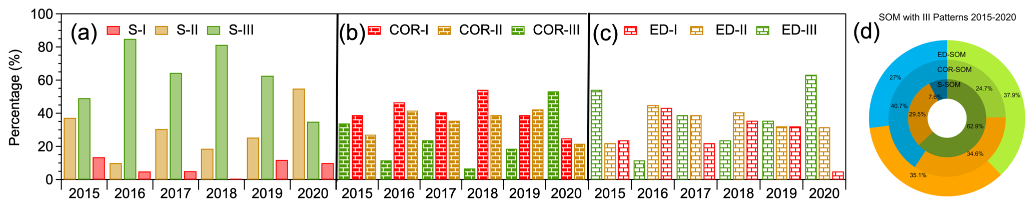
Figure 5 Cluster size distributions identified by S-SOM (inner ring), COR-SOM (middle ring), and ED-SOM (outer ring) over the years 2015–2020 (d) and cluster days in each year. (a) S-SOM, (b) COR-SOM, and (c) ED-SOM.

In terms of structure characteristics of clustering number distribution for S-SOM, three-node SWPs (Fig. 4) and seven-node SWPs (Fig. S13) were regarded as being the optimal numbers of SWPs after checking the clustering number distribution for each run. From the top panel of Fig. 4, three types of SWPs identified by S-SOM demonstrate that NCP, YRD, NEC, and NWC are under the control or influence of different high-pressure systems. For seven-node SWPs identified by S-SOM, even though the high-pressure system varies in numbers and locations, some patterns (Fig. S13d and e) still have a relatively high similarity, which might be attributed to the over-splitting or a dataset that is too short to capture the full climatology. Overall, the result of the three-node SWPs of S-SOM is thus identified as the best solution to study the haze event in China in further detail.

3.3 Impact of weather elements on PM_2.5 and O₃ under the SWPs

To better understand the regional influence of different SWPs on PM_2.5 and O₃ concentration levels, NCP and NEC (SC), which have higher (lower) than expected concentrations for PM_2.5 (O₃) and have more measurement stations as well, were selected as the research domains. To investigate the cause of the unexpected PM_2.5 and O₃ variations with respect to climatology, a comparison of the identified three-node SWPs is made between the days of 2020 and 2015–2019. As shown in Fig. 6 and as detailed in Figs. 7–9, pattern I in 2020 (Fig. 6d) shows a north coastal high-pressure circulation system, located in the Yellow Sea, which is enhanced from that in 2015–2019 (Fig. 6a) and influences the NCP and NEC regions (see Figs. 7a, d–f and 8a, d–f) more strongly from the southeast direction with a generally warmer and, in the case of NEC, also faster airflow. The double-centre high-pressure system in pattern II is strengthened in 2020 (Fig. 6e) and located in the region of Mongolia and the Bohai Sea in China compared to 2015–2019 (Fig. 6b). This brings along a more stagnant, i.e. low speed and cold, but also extremely wet northern airflow controlling the NCP region (Fig. 7a, d–f) and a moderately wetter airflow dominating the NEC region (Fig. 8a, d–f). Pattern III, on the other hand, shows a much weakened Siberian high and a missing China north coastal high in 2020 (Fig. 6f), when compared to a pattern exhibiting two high-pressure centres during the 2015–2019 reference period (Fig. 6c). This leads to a generally warmer, slightly faster, and more humid airflow to the NCP (Fig. 7a, d–f) and NEC (Fig. 8a, d–f) regions. For SC, which is always located at the southernmost part of the observed high-pressure centres (Fig. 6), and for all three patterns, only small changes are seen in 2020 compared to the 2015–2019 time period with a more easterly component in the winds (Fig. 9a–c), leading to slightly warmer and (except for pattern III) moister airflow (Fig. 9d–f).

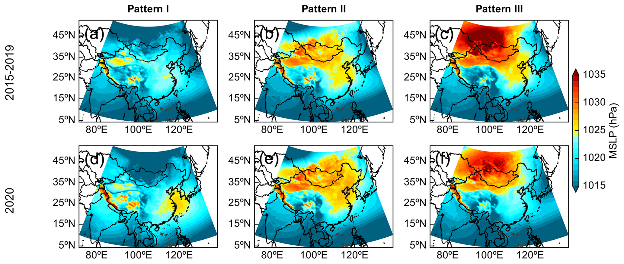
Figure 6 Comparison of the three weather patterns between cluster days in 2020 (d, e, f) and 2015–2019 (a, b, c), respectively.

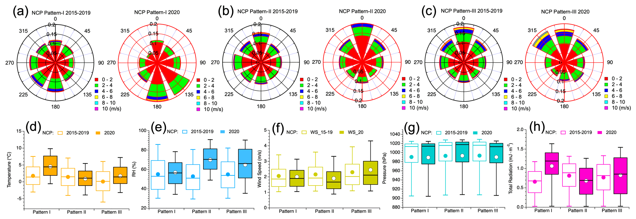
Figure 7 Comparisons of different weather factors (including wind speed, wind direction, temperature, relative humidity, pressure, and total radiation) between cluster days in 2020 (red wind rose and solid box-and-whisker plots) and in 2015–2019 (black wind rose and hollow box-and-whisker plots) for the three weather patterns in NCP.

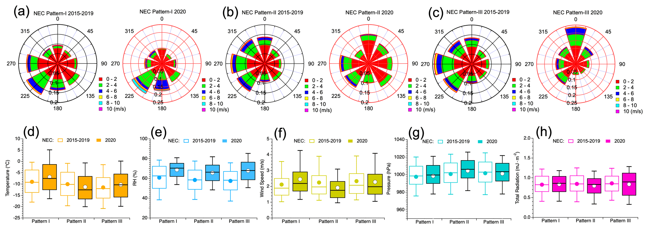
Figure 8 Comparisons of different weather factors (including wind speed, wind direction, temperature, relative humidity, pressure, and total radiation) between cluster days in 2020 (red wind rose and solid box-and-whisker plots) and in 2015–2019 (black wind rose and hollow box-and-whisker plots) for the three weather patterns in NEC.

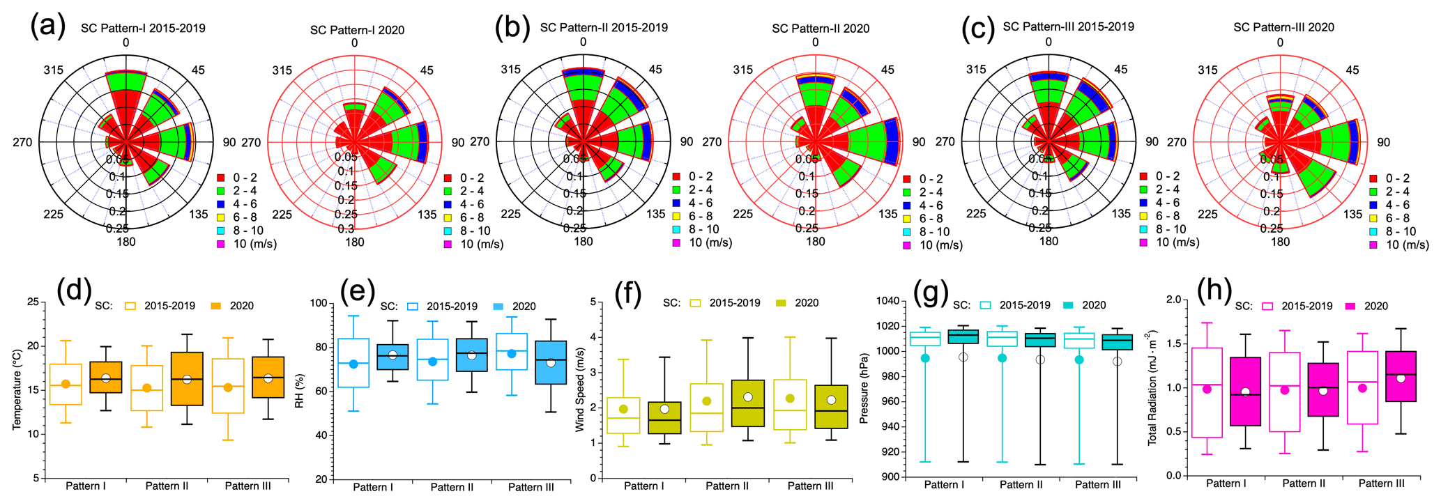
Figure 9 Comparisons of different weather factors (including wind speed, wind direction, temperature, relative humidity, pressure, and total radiation) between cluster days in 2020 (red wind rose and solid box-and-whisker plots) and in 2015–2019 (black wind rose and hollow box-and-whisker plots) for the three weather patterns in SC.

We now turn to the discussion of the observed distributions of PM_2.5 and O₃ (Fig. 10) aggregated over the three SWPs and the regions of NCP, NEC, and SC for the 2020 and the 2015–2019 time periods, respectively. For PM_2.5 in NCP (Fig. 10a), the mean values in patterns I, II, and III in 2015–2019 all remained at high pollution levels with values of 96.4, 92.6, and 87.7 µg m⁻³, respectively. In contrast, due to the anthropogenic emissions reductions during the lockdown period in 2020, the PM_2.5 mean values for patterns I and III decreased to 68.8 and 59.8 µg m⁻³, even when coupled with a positive RH climatological anomaly (Fig. 7e: 2 % and 10 %), which could be conducive to generating additional PM_2.5 generally. Unlike patterns I and III, the PM_2.5 mean value in pattern II 2020 surprisingly keeps at an equivalent level (92.5 µg m⁻³) to pattern II in 2015–2019 (92.6 µg m⁻³) under a weather condition of a combination of the greatest RH anomaly (Fig. 7e; 17 %) and a negative WS anomaly (Fig. 7f; −0.3 m s⁻¹), which offsets the contribution from the emissions reduction in NCP. For O₃ in NCP (Fig. 10d), patterns I and III in 2020 exhibit greater temperature anomalies (Fig. 7d; 2.7 and 2.9 °C, consistent with higher total radiation levels; see Fig. 7h) and thus facilitate additional O₃ generation (20 and 13 µg m⁻³). Pattern II in 2020 with a negative temperature anomaly (−0.1 °C, consistent with lower total radiation levels; see Fig. 7h) favours a more moderate O₃ increase (3 µg m⁻³).

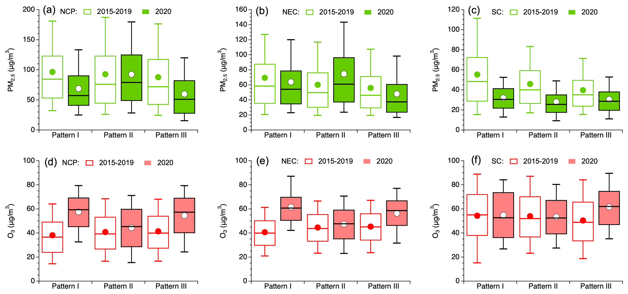
Figure 10 Comparisons of PM_2.5 (green colour) and O₃ (red colour) between cluster days in 2020 (filled box-and-whisker plots) and in 2015–2019 (hollow box-and-whisker plots) for the three weather patterns in NCP (a, d), NEC (b, e), and SC (c, f).

In the NEC region, the maximum PM_2.5 increase (15 µg m⁻³) occurred under the influence of pattern II in 2020 (Fig. 10b), with a negative wind speed anomaly (Fig. 8f; −0.3 m s⁻¹) when compared to the same pattern in 2015–2019, indicating that the meteorological effect acts in the opposite way to the emission reductions during the COVID-19 lockdown period. Without an offsetting effect from the unfavourable meteorological conditions, mean values of PM_2.5 for patterns I and III in 2020 decreased by 5 and 8 µg m⁻³, respectively. For O₃ (Fig. 10e), unlike a negative temperature anomaly (Fig. 8d; −1.3 °C) in SWP II, both higher O₃ increases in SWPs I (11 µg m⁻³) and III (11 µg m⁻³) compared to that in SWP II (2 µg m⁻³) are driven by positive temperature anomalies (Fig. 8d; 2 and 4.4 °C).

In the SC region, without an extreme weather element anomaly facilitating additional PM_2.5 production, PM_2.5 mean values for all three SWPs in 2020 are at a lower level than in 2015–2019 (Fig. 10c) and attributable to the emissions reductions during the COVID-19 lockdown. Higher precipitation levels in 2020 than during the 2015–2019 period also helped reduce PM_2.5 levels (see Figs. 3c and S14). For O₃ (Fig. 10f), a negative RH anomaly (Fig. 9e) for SWP III in 2020 led to the greatest O₃ elevation for this region. On the other hand, the O₃ in pattern I is found to remain at similar levels during both time periods since no significant differences in the weather patterns are found. Finally, a positive wind speed anomaly (Fig. 9f; 0.21 m s⁻¹) is conducive to an unusual O₃ decline (−0.5 µg m⁻³) in SWP II in 2020 when compared to 2015–2019, which is contrary to the O₃ situation under the effect of all other SWPs discussed above.

Overall, we found that the unexpected PM_2.5 pollution increase in NCP and NEC and an O₃ decline in SC occur simultaneously but only during SWP II, which is equivalent to the situation found in the observations during the haze event. When we further investigate the calendar occurrences of the three different SWPs (Fig. S15), it is indeed found that 70 % of the haze days were associated with SWP II. This finding thus indicates that SWP II can be regarded as the representative weather pattern which best explains the cause of the unexpected haze and O₃ decline events.

3.4 Predominant meteorological factors for PM_2.5 and O₃ pollution

After identifying which SWP could control the impact of each weather element on the PM_2.5 and O₃ levels, as observed during the haze event in 2020, we further use machine learning coupled with the SHAP approach to quantify the impact of each weather element on the PM_2.5 and O₃ under the business as usual (hereafter referred to as BAU) emission strength scenario during the haze event in 2020. This BAU scenario thereby is constructed by the gradient-boosting machine that trained the model using historical features to predict the future-dependent features without considering the huge emission reduction due to the COVID-19 lockdown. It is a counterfactual scenario assuming that the emission strength is the same as the BAU. In our previous study, the GBM model was applied to train daily data over 2015–2019 and predict six air pollutants including PM_2.5 and O₃ over the first 3 months of 2020 in 367 cities across China (Shen et al., 2022). The good performance of the GBM model was measured by achieving relatively high Pearson correlation coefficients (PCCs) and lower root mean squared errors (RMSEs) for the final predictions of PM_2.5 and O₃ (details can be found in the Supplement). Figures 11a, d, and g and S16 show the time series results in the first 2 months for PM_2.5 and O₃ between the observation and prediction in NCP, NEC, and SC, respectively. We find that the predictions generally agree well with the observations with reasonably high PCCs (NCP 0.7, NEC 0.6, and SC 0.8), indicating the good performance of the GBM model. Note that these predictions might be with high RMSEs due to the input being the BAU emissions instead of the lockdown emission reduction. Many studies have estimated PM_2.5 and O₃ using different prediction models, but they are limited to explain the final predictions (Xiao et al., 2018; Zhang et al., 2021; Jin et al., 2022), especially to provide details of specific input features (Weng et al., 2022). In our study, the SHAP module coupled to the GBM model was run to quantify the importance of the input variables during the haze event in 2020 (Fig. 11b, e, and h). On average, in the BAU scenario, the SHAP value of the time variables, including CNY, DOW, holidays, and JD, have no impact or negative impacts on PM_2.5 and O₃ (Fig. 11c, f, and i). For meteorological elements that enhanced the production of PM_2.5, temperature ranked first among the six meteorological elements during the haze event, followed by RH, WS, and pressure in NCP versus WS, pressure, and RH in NEC, respectively. In terms of the positive SHAP values of temperature, pressure, RH, and WS in PM_2.5 predictions, it reveals that those meteorological features push PM_2.5 prediction to a higher value, suggesting that the final predictions were up to the baseline concentrations in NCP and NEC. In SC (Fig. 11i), positive mean SHAP values (2.2 µg m⁻³) for RH would be conducive to additional ozone generation due to the relatively lower values compared to before the haze event (Fig. 11g), thus pushing the predicted ozone higher. In contrast, a negative mean SHAP value (−5.5 µg m⁻³) for temperature during the haze event (Fig. 11i) would suppress ozone production attributable to smaller mean values, thus leading to a lower-ozone prediction. It should be noted that RH with a higher absolute SHAP value (9.8 µg m⁻³) exceeding temperature (−6.7 µg m⁻³) became the primary factor dominating the high-ozone level from 27 January to 2 February 2020. It is attributed to the SWP II in SC (Fig. 9d, f) with strong moist winds from the ocean, leading to the importance of RH surpassing temperature, which is consistent with the previous study (Weng et al., 2022). However, over the full period of the haze event, the negative effect of temperature dominated a higher-ozone level during the haze event based on the larger absolute SHAP value for temperature. The weaker than expected decrease in ozone as response to a lower temperature might be attributed to the emission reductions in the ozone precursors due to the COVID-19 lockdown measures. When we investigate the observed weather elements in 2020 against that averaged over 2015–2019, we can find that NCP and NEC were both under the control of SWP II, with lower temperatures and a higher RH, which facilitated the formation of PM_2.5. Meanwhile, the SC region was influenced by the SWP II with higher temperatures, higher RH, and higher WS weather conditions, resulting in a decline in the O₃ in climatology but a relative high-ozone level in prediction from the SHAP explanation. Overall, we can not only find the impact of weather elements on PM_2.5 and O₃ in the prediction scenario and in climatology, but we can also conclude that temperature plays a key role in such an impact.

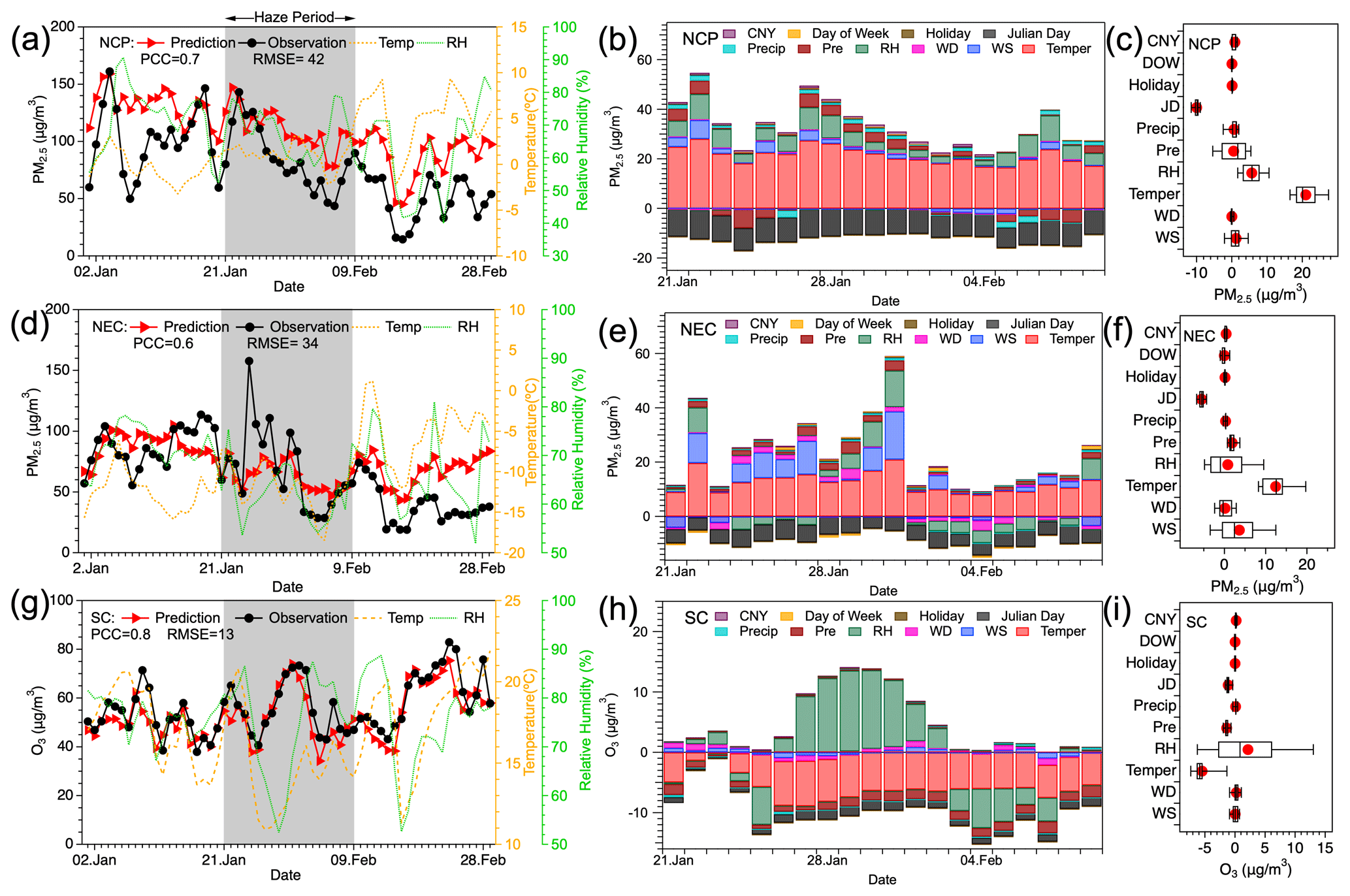
Figure 11 Time series comparisons between observations (dotted black line) and predictions (triangled red line) combined with the SHAP values of the input variables (colourful bar) for the PM_2.5 and O₃ predictions in NCP (a, b), NEC (d, e), and SC (g, h), respectively (note that the box-and-whisker plots represent the mean SHAP value of the input variables during the prediction in NCP (c), NEC (f), and SC (i), respectively, and the shaded area (a, d, g) indicates the haze event period).

4 Conclusion

At the beginning of the COVID-19 pandemic, China suspended almost all non-essential human activities. However, serious haze pollution still occurred in North China during this period, triggering extensive investigations. On the other hand, while O₃ concentrations were increasing across almost all of China due to the shift in the chemical regime, the SC region exhibited a decrease in O₃. To further understand the role of meteorology in regulating air pollution during this period, we investigated in more detail the role of synoptic-scale weather patterns in driving the meteorology in these regions of China. To this end, we first determined the optimal approach for identifying synoptic-scale weather patterns out of three self-organising map methods. With the S-SOM method yielding the most optimal results, we then analysed the variation in the each meteorological factor under the control of the weather type that produces anomalous PM_2.5 concentrations in the NCP and NEC and anomalous O₃ concentrations in SC. Finally, we quantified the importance of each meteorological factor assuming a BAU scenario through a machine learning model coupled with a SHAP module.

The large-scale double-centre high-pressure system was identified by the optimal S-SOM method with a low-speed, cold, and extremely wet northern airflow controlling the NCP region; a low-speed, warm, and wet airflow from the Bohai Sea dominating the NEC region; and warmer air masses covering the SC region simultaneously. The above weather element anomalies controlled by the large-scale high-pressure system could well explain the unexpected PM_2.5 pollution and O₃ decline in climatology in NCP, NEC, and SC, respectively.

Moreover, the SHAP results indicate that, in the BAU scenario, the time series trend of PM_2.5 and O₃ have a high similarity with that of the observations, indicating a good performance of the prediction model (despite the differing emissions). The SHAP results stress the impact of meteorological conditions on PM_2.5 and O₃ and further quantify the importance of each weather element under the specific weather system, revealing the most important role that temperature played in PM_2.5 pollution in NCP and NEC and in high O₃ level (note that this has to be understood relative to a lower-ozone level compared to climatology) in SC, respectively.

Overall, this study provides a potential way to understand the synergistic effects of various meteorological factors in reducing pollution and to quantify the importance of each weather element as well. As a result, the provision of information on what role each weather element plays in unexpected air pollution cases can help policymakers to implement air pollution control strategies. However, our work will have to be expanded further and add more related meteorological factors to the GBM model to improve its performance. In fact, more studies should focus on the topic of understanding the impact of meteorology on different air pollutants in particular due to weather conditions in a changing climate.