the Creative Commons Attribution 4.0 License.
the Creative Commons Attribution 4.0 License.
 | 30 May 2024
Surface networks in the Arctic may miss a future methane bomb
Sophie Wittig
Antoine Berchet
Isabelle Pison
Marielle Saunois
Jean-Daniel Paris
The Arctic is warming up to 4 times faster than the global average, leading to significant environmental changes. Given the sensitivity of natural methane (CH4) sources to environmental conditions, increasing Arctic temperatures are expected to lead to higher CH4 emissions, particularly due to permafrost thaw and the exposure of organic matter. Some estimates therefore assume the existence of an Arctic methane bomb, where vast CH4 quantities are suddenly and rapidly released over several years. This study examines the ability of the in situ observation network to detect such events in the Arctic, a generally poorly constrained region. Using the FLEXPART (FLEXible PARTicle) atmospheric transport model and varying CH4 emission scenarios, we found that areas with a dense observation network could detect a methane bomb occurring within 2 to 10 years. In contrast, regions with sparse coverage would need 10 to 30 years, with potential false positives in other areas.
- Article
(4529 KB) - Full-text XML
- Companion paper
-
Supplement
(8834 KB) - BibTeX
- EndNote


Arctic warming is proceeding 3 to 4 times faster than the global average. (AMAP, 2021; Rantanen et al., 2022). As a consequence, various environmental changes can be observed in high northern latitudes, triggering climate feedbacks that potentially accelerate global warming even further (AMAP, 2021). These feedbacks include, for instance, increased greenhouse gas emissions (e.g. Treat et al., 2015), especially in the form of methane (CH4). In the Arctic, CH4 emissions are generally dominated by natural sources (e.g. Saunois et al., 2020; AMAP, 2015), including high northern latitude wetlands and other freshwater systems, fluxes from various oceanic sources, forest fires and geological fluxes. Quantifying natural CH4 sources in the Arctic remains challenging and estimates are subject to large uncertainties. According to Saunois et al. (2020), wetland emissions above 60° N amount to 7 to 16 Tg CH4 yr−1 and other natural sources to 2 to 4 Tg CH4 yr−1. However, as the Arctic region is not uniformly defined, comparing different estimates from various studies is an additional challenge. Since these natural CH4 sources are sensitive to the surrounding environmental and climate conditions, it is assumed that CH4 emissions will increase with progressing Arctic warming (e.g. AMAP, 2015).
This predicted increase is predominantly connected with permafrost thawing and the resulting exposure of large pools of degradable organic matter (Whiteman et al., 2013; Glikson, 2018). Regarding terrestrial permafrost, estimates predict that until 2100, up to 274 Pg of carbon could be released to the atmosphere, with CH4 accounting for 40 % to 70 % of the permafrost-affected radiative forcing (Schneider von Deimling et al., 2015; Walter Anthony et al., 2018). A potential increase in methane emissions from high northern latitude wetlands due to thawing permafrost soils has been postulated, e.g. by Schuur et al. (2015).
Several studies have highlighted the importance of CH4 emissions from the Arctic Ocean, particularly in shallow waters underlain by permafrost (Damm et al., 2010; Kort et al., 2012). Subsea permafrost thaw has been observed in the ESAS (East Siberian Arctic Shelf) and the importance of this region has been highlighted, for instance by Shakhova et al. (2015, 2019) and Wild et al. (2018). Future estimates suggest that around 50 Gt of methane could be released from gas hydrates in the ESAS alone over the next 50 years (Shakhova et al., 2010), consistent with present annual estimates (e.g. Berchet et al., 2016).
Methane emissions from anthropogenic sources are estimated to be around at around 2 to 10 Tg CH4 yr−1 (Saunois et al., 2020). Anthropogenic CH4 emissions in the Arctic are not explicitly assumed to increase in the future and several Arctic states report decreases in future emissions (Arctic-Council, 2019). However, the large estimates of unexplored fossil fuel resources make this region potentially attractive for future drilling campaigns (Gautier et al., 2009), and it has been confirmed that drilling has increased over the past decades in Arctic-boreal regions (Klotz et al., 2023).
The magnitude and multiplicity of possible climate feedbacks related to Arctic CH4 natural emissions have been dramatically called a sleeping giant, (Mascarelli, 2009), a methane time bomb (Glikson, 2018) or even the methane apocalypse (Ananthaswamy, 2015). However, different studies assessing an imminent Arctic methane bomb are more optimistic. McGuire et al. (2018) concluded that significant net carbon losses from northern permafrost regions will only occur after 2100, assuming effective climate action. Anisimov and Zimov (2021) demonstrated that CH4 emissions from Siberian wetlands will increase by less than 20 Tg yr−1 by 2050, leading to a global temperature increase of less than 0.02 °C. Kretschmer et al. (2015) showed that CH4 emissions from the ocean will remain limited over the next century despite significant losses of methane hydrates, particularly in the Arctic Ocean. Finally, Schuur et al. (2022) concluded that a sudden Arctic methane bomb, releasing overwhelming quantities of CH4 into the atmosphere in a short period of time, is not currently supported by observations or projections.
In Wittig et al. (2023), we used the existing network of atmospheric CH4 concentrations in the Arctic in an inverse modelling system and concluded that no significant trend was observable in the last decade. Apart from the likelihood of an Arctic methane bomb in the near future, the objective of this study is to analyse the capability of a stationary observation network of atmospheric CH4 concentrations to properly detect such a possible event in the future using atmospheric inversion. This is motivated by the general sparsity of the current (and planned) observation network in the Arctic. A methane bomb is characterised in our study as a sudden and steep increase in methane emissions, releasing large quantities of CH4 over several years. We focus here on the years 2020 to 2055. Consequently, this study aims to discuss the following questions: (i) could future increases of CH4 emissions in the form of an Arctic methane bomb be accurately detected by the current observation network? and (ii) what improvements in the detectability of CH4 emissions can be achieved by a hypothetically expanded network?
In order to implement this work, we apply hypothetical trend scenarios on different CH4 emission sources to simulate a methane bomb in different regions located in high northern latitudes. By combining these emission scenarios with the extrapolated output of an atmospheric transport model, we obtain synthetic CH4 mixing ratios for the current observation network in the Arctic and sub-Arctic as well as for an observation network extended by possible additional sites. These synthetic observations subsequently serve as input data for the inverse modelling set-up in order to identify a temporal threshold of possible detection and to analyse regional differences in the ability of the two networks to adequately detect and localise increasing CH4 emissions. Since we assume optimum quality and availability of the measurement data, the results obtained represent a best-case scenario for the detection of an Arctic methane bomb using exclusively in situ observations.
Here, we implement an analytical inversion, aiming at explicitly and algebraically finding the optimal posterior state of a system xa and the corresponding uncertainties Pa. This approach is defined by
with K the Kalman gain matrix given by
Our inversion system optimises CH4 fluxes region-wise (121 regions, shown in Fig. 1, Sect. 3.1) over a pan-Arctic domain, using atmospheric CH4 concentrations. Our study examines scenarios spanning 36 years (2020–2055) to find a trade-off between computational cost and the importance of the decadal timescale for climate change. For computational reasons, this period has been split into 36 independent 1-year inversion windows, which are computed separately.
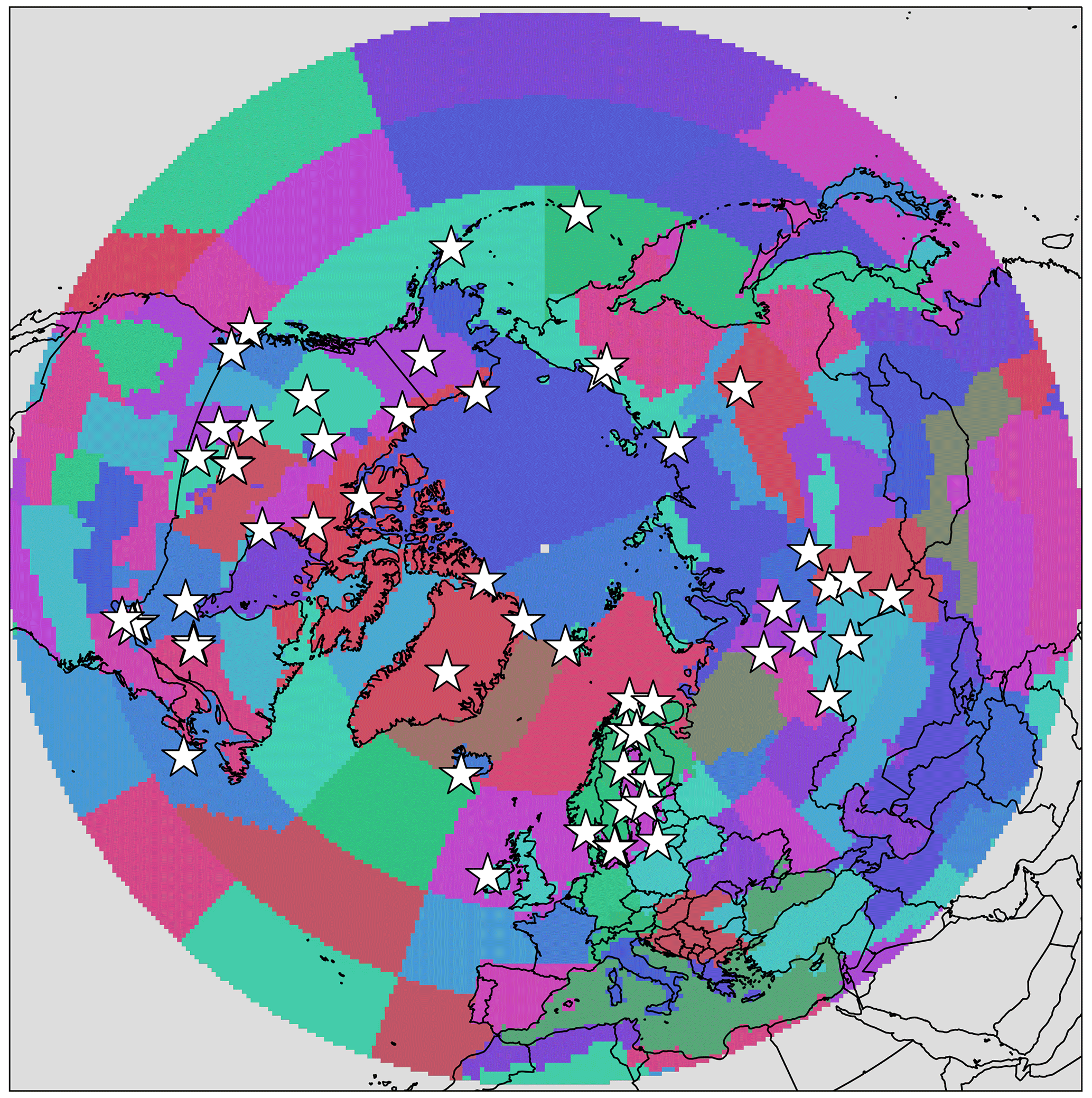
Figure 1Regional Carbon Cycle Assessment and Processes (RECCAP) regions above 30° N. The white stars indicate all observation sites used in this study.
The prior knowledge of the state, in this case surface fluxes and soil uptake of CH4, is defined by the control vector xb (see Sect. 3.3). Here, xb also contains information on the initial CH4 background mixing ratios (described in Sect. 3.4), which are therefore optimised in addition to the CH4 fluxes. The corresponding uncertainties are specified in the prior error covariance matrix B. We use B matrices based on the Monte Carlo log-likelihood approach developed in Wittig et al. (2023). The off-diagonal elements of the prior error covariance matrix are thereby determined by applying spatial and temporal correlations of 500 km and 7 d respectively.
The observation operator is assumed to be linear since chemical oxidation of CH4 by free radicals in the atmosphere is neglected for this application. It is therefore defined as its Jacobian matrix H and contains the simulated equivalents of the observations (further described in Sect. 3.4 and illustrated in Fig. S2).
In classical inverse modelling approaches, the observation vector yo contains available observations, e.g. of CH4 mixing ratios. However, in this work we want to study different future scenarios of CH4 emissions and therefore it is not possible to use actual measurements. Therefore, we simulate synthetic observations of CH4 mixing ratios based on different emissions scenarios (further described in Sect. 3.5).
For a given emission scenario, the true state (hereafter called truth) of the CH4 emissions over the future period of simulation is defined as xt and changes with a given trend k, which is constant throughout all the years within the period of interest. This trend was only applied from the second year of the study period (2021); in the year 2020 the truth is identical to the prior state. The observations vector for a given year j can then be calculated as
In our analysis of the detectability of elevated Arctic CH4 emissions (Sect. 4), we examine how accurately the truth is captured in the posterior emissions of different regions and whether these elevated fluxes are localised in the right area. By design, our inverse modelling system will try to fit additional fluxes by adding CH4 emissions in the Arctic region but possibly not at the correct location. Since, as described above, the background mixing ratios are also included in the control vector xb and consequently optimised in the posterior state, it is likely that part of the missing CH4 mass is compensated for by increased posterior background concentrations. Therefore a small bias in the posterior emissions is generated.
Similarly to the prior uncertainties, the matrix R containing the uncertainties in the synthetic observations as well as the modelled CH4 mixing ratios is based on Wittig et al. (2023). Theoretically, the synthetic observations should be perturbed by an error (with a Gaussian distribution, following the matrix R), accounting for measurement errors, as well as other uncertainties such as transport and aggregation (e.g. Szénási et al., 2021). In our approach, we deliberately disregard these errors in order to obtain optimistic results and assimilate optimal measurements to analyse the best possible detection of different observation networks (Sect. 3.2) regarding a methane bomb event.
3.1 Region under study
For the implementation of the inversion, observation sites in high northern latitudes displaying different observation networks have been included in this study (see Sect. 3.2). To represent concentrations at these sites as accurately as possible, we simulate the influence of fluxes from a buffer region above 30° N. This region is subsequently divided into 121 sub-regions, as proposed by the Regional Carbon Cycle Assessment and Processes (RECCAP; Ciais et al., 2022) initiative, in order to better detect local differences. Figure 1 shows the resulting sub-regions as well as all the included observation sites (indicated with white stars).
3.2 Observation networks
As described in Sect. 2, the observations used for the inverse modelling approach are based on synthetic CH4 mixing ratios assuming different emission scenarios. We use, however, an existing network of measurement sites located in high northern latitudes. In this study, we focus exclusively on stationary CH4 measurements, as our period of study spans several decades. Other types of greenhouse gas measurements, such as satellite observations, are currently limited to providing data for only a few years and are therefore not suitable for our purposes. The corresponding stations include both continuous and discrete measurements. To simulate an “optimal” observation network, we assume that all of those observation sites provide continuous measurements.
Two different network scenarios are used for this study. The first one, from here on referred to as current, includes all observation sites with available data of CH4 mixing ratios during recent years. The term current refers here only to the location of the stations. This network, as used in this study, already provides additional data compared to the actual observations available from these sites. This is because, as stated before, we assume continuous measurements where currently only discrete measurements are carried out. The current network contains 40 stations in total, whereby the majority (26 sites) of the sites is located in North America (Canada, USA and Greenland). Ten observation sites are located in the Russian Arctic and sub-Arctic and four sites in northern and western Europe (Finland, Norway, Ireland and Iceland). The second network, referred to as extended, includes additional observation sites in high northern latitudes. The extended network expands the current network by 16 observation sites. The majority of these stations, 11, are located in northern Europe (Sweden, Finland, Norway, Lithuania and eastern Russia), 3 in central and western Russia and 1 station each in Canada and Greenland.
Both the current and extended networks were selected based on their theoretical provision of CH4 observations, including measurements in the Russian Arctic that may currently not be accessible to the scientific communities of certain countries, as we believe it is important to conduct this work outside of ongoing political conflicts.
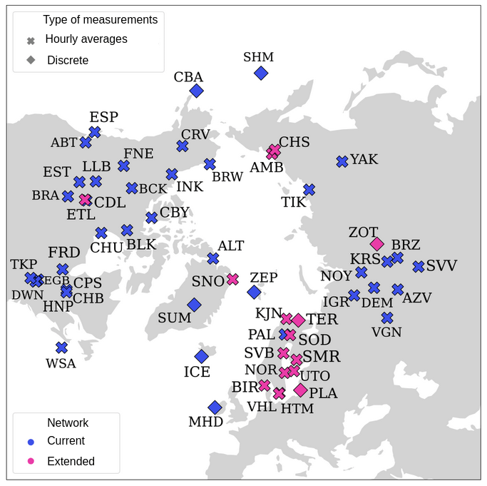
Figure 2Location of observation sites used to generate synthetic mixing ratio data. The current network is shown in blue, the additional stations in pink. Crosses indicate quasi-continuous measurements, diamonds discrete measurements. The types of measurements refer to the measurements that are currently taking place at these sites, whereas in this study we assume all measurements to be continuous.
The different observation networks are shown in Fig. 2 and an overview of both observation networks can be found in the Supplement in Table S1 (current network) and Table S2 (extended network).
The extended network here contains observation sites where measurements of atmospheric CH4 concentrations are (i) only available for years starting in 2022, (ii) no longer taking place, (iii) where the measurement data are not publicly available, (iv) where the stations use ground-based remote sensing instruments to obtain total column measurements of CH4 or (v) where CH4 is currently not measured at all but measurements of other trace gases or air pollutants are taking place. As the observation network is limited at high northern latitudes, these additional stations were added to investigate what benefits a reasonably realistic extended network might offer for constraining methane fluxes.
3.3 Prior CH4 emissions
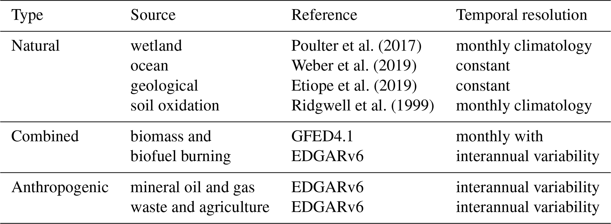
The different methane sources and sinks used as prior information are based on a set of different emission inventories and land-surface models. Natural methane sources include here emissions from high-northern latitude wetlands, geological fluxes, CH4 emissions from the Arctic Ocean and wildfire events.
The CH4 emissions related to anthropogenic activities include the exploitation and distribution of natural gas and mineral oil, agricultural activities, waste management and biofuel burning. Since anthropogenic activities are generally limited in the Arctic and sub-Arctic, the corresponding data sets have been combined for simplification.
As mentioned before, atmospheric CH4 sinks from free radicals are not taken into account. However, soil oxidation due to microbial activities is included in the form of negative CH4 emissions. All prior estimates are listed in Table 1
Poulter et al. (2017)Weber et al. (2019)Etiope et al. (2019)Ridgwell et al. (1999)Table 1Methane sources and sinks taken into account in the prior emissions.
3.4 Synthetically generated CH4 mixing ratio data
The modelled CH4 mixing ratios are obtained by simulating backward trajectories of virtual particles using the Lagrangian atmospheric transport model FLEXPART (FLEXible PARTicle) version 10.4 (Stohl et al., 2005; Pisso et al., 2019).
In this study, 2000 particles are released once per day at each observation site (Sect. 3.2) and followed 10 d backwards in time. The horizontal resolution is here 1° × 1°. The meteorological input data for the FLEXPART simulations are provided by the European Centre for Medium-Range Weather Forecasts (ECMWF) ERA5 (Hersbach et al., 2020) with 3-hourly intervals and 60 vertical layers.
The footprints obtained by sampling the near-surface residence time of the various backward trajectories of the virtual particles are subsequently used to determine the CH4 mixing ratios per methane emission sector (Sect. 3.3) and sub-region (Sect. 3.1). The footprints define here the connection between the methane fluxes discretised in space and time and the change in concentrations at the observation site (Seibert and Frank, 2004). To obtain a time series of modelled CH4 mixing ratios, a time series of footprints is integrated with discretised CH4 flux estimates.
As described in Sect. 2, in the inverse modelling framework, the modelled CH4 mixing ratios obtained from the FLEXPART footprints are included in the observation operator H. In this study, this matrix is used for both the calculation of the synthetic future observations (shown in Eq. 3) based on future emission scenarios (see Sect. 3.5) as well as their modelled equivalents based on prior emission estimates.
Since the thus obtained CH4 mixing ratios only display short-term fluctuations at the observation sites, the background mixing ratios need to be taken into account. These are calculated by combining a CH4 concentration field as initial condition with the FLEXPART backward simulations (e.g. Thompson and Stohl, 2014; Pisso et al., 2019). The initial concentration field is provided by the Copernicus Atmospheric Monitoring Service (CAMS): a CH4 mixing ratio field from CAMS global reanalysis EAC4 (ECMWF Atmospheric Composition Reanalysis 4) with 60 vertical layers, a 3-hourly temporal resolution and a 0.75° × 0.75° spatial resolution has been used (Inness et al., 2019). The implementation used for obtaining the background mixing ratios is provided by the Community Inversion Framework (CIF; Berchet et al., 2021a). However, since an exact estimate of the background mixing ratios remains challenging and the calculated background concentrations do not provide perfect estimates, the background mixing ratios are optimised together with the CH4 fluxes (see Sect. 2).
As mentioned in Sect. 3.1, the period under study covers the years 2020 to 2055. To represent this period of time, which partly lies in the future, we use FLEXPART simulations covering 12 years (between 2008 and 2019) and string together this sequence of footprints three times in a row. It is here assumed that the climatology of atmospheric transport and fluxes does not change significantly in the 36 years following the year 2019.
3.5 Future emission scenarios
We create various scenarios by varying four different parameters: (i) CH4 emission sources, (ii) the trend in these sources, (iii) the regions in which the trends are applied and (iv) the observation network.
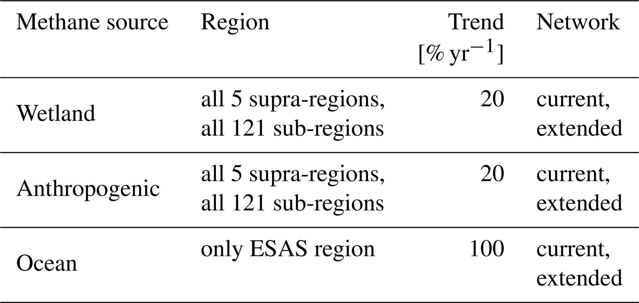
Hypothetical trends are applied, in varying regions, to wetlands, anthropogenic activities and the Arctic Ocean (Table 2). We define five supra-regions (see Supplement, Fig. S1): the Arctic, the combined Arctic and sub-Arctic (hereafter named entire region), North America, East Eurasia and West Eurasia; the last three regions only cover high northern latitude areas within those continents. Additionally, 121 sub-regions are defined as detailed in Sect. 3.1. In total, the trends are therefore applied to 126 different regions including both the sub- and the supra-regions.
For each of these zones, positive trends are applied separately to wetland and anthropogenic emissions. Oceanic CH4 emissions are only increased in the sub-region that contains the ESAS, as these are difficult to detect with the surface networks.
The trends are varied between a 0.1 % and 20 % increase per year for anthropogenic and wetland emissions and between 1 % and 100 % increase per year for oceanic sources. As the results obtained are applicable to both lower and higher trend scenarios, we focus only on the highest selected increase (20 % for wetlands and anthropogenic sources and 100 % for oceanic fluxes), as this is also the most representative for a methane bomb event.
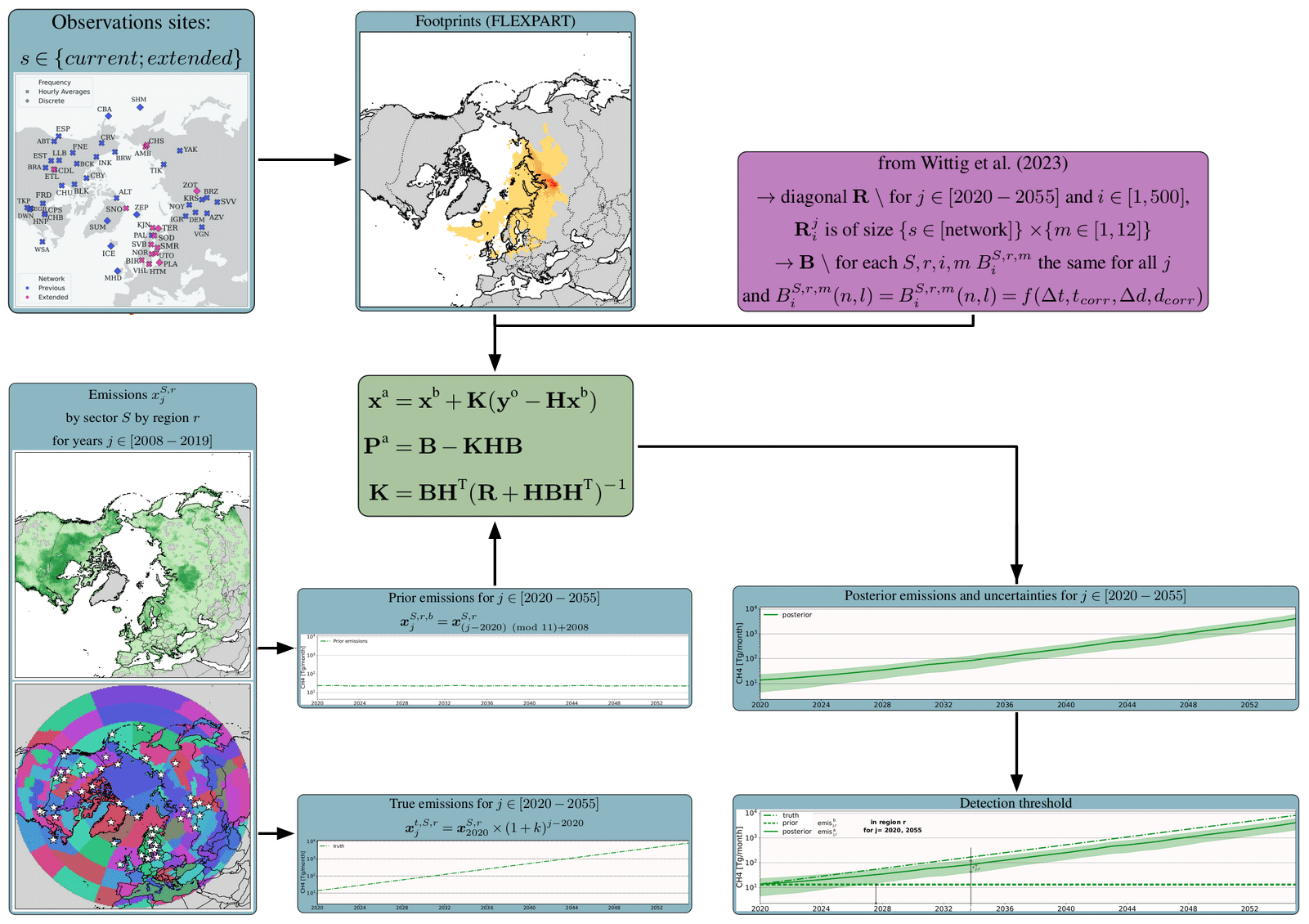
Figure 3Principle of the inversion set-up used in this study. The modelled input and output data of the inversion are shown in the blue boxes, the respective uncertainties in the purple box and the optimisation strategy in the green box. See Sect. 2 and Wittig et al. (2023) for full details.
For both anthropogenic and wetland emissions we obtain 252 separate scenarios when increasing the emissions in each of the 126 regions and using the two different observation networks. Since oceanic fluxes are only increased in one region, we obtain only two scenarios using the different observation networks. This results in 506 different set-ups with corresponding synthetic observations. Hence, the same number of inversions are carried out. The main elements for the ensemble of inversions run in this study are summarised in Fig. 3 and detailed in Sect. 2.
Table 2The different scenarios providing the simulated observations.
Section 4.1 illustrates how the true and the posterior fluxes evolve over time in the Arctic for one selected scenario. We evaluate the performance of the inversion through examining not only how close to the true fluxes the posterior fluxes become but also the time at which a trend appears in the posterior fluxes compared to the flat prior. This is described in Sect. 4.2.
4.1 Comparison of truth and posterior state over time
In order to evaluate how well the anticipated trends in the different regions are captured over the whole period of interest, the time series of the true and posterior states are compared to each other. The true state refers here to the emission scenario used to compute the synthetic observations. Figure 4 shows the time series of wetland and total CH4 emissions between the years 2020 and 2055 in different supra-regions (North America, East Eurasia and the Arctic) as well as the total CH4 emissions for the entire region. The truth is here a 20 % increase in wetland emissions only in the supra-region East Eurasia, and the extended observation network was used for the inversion.
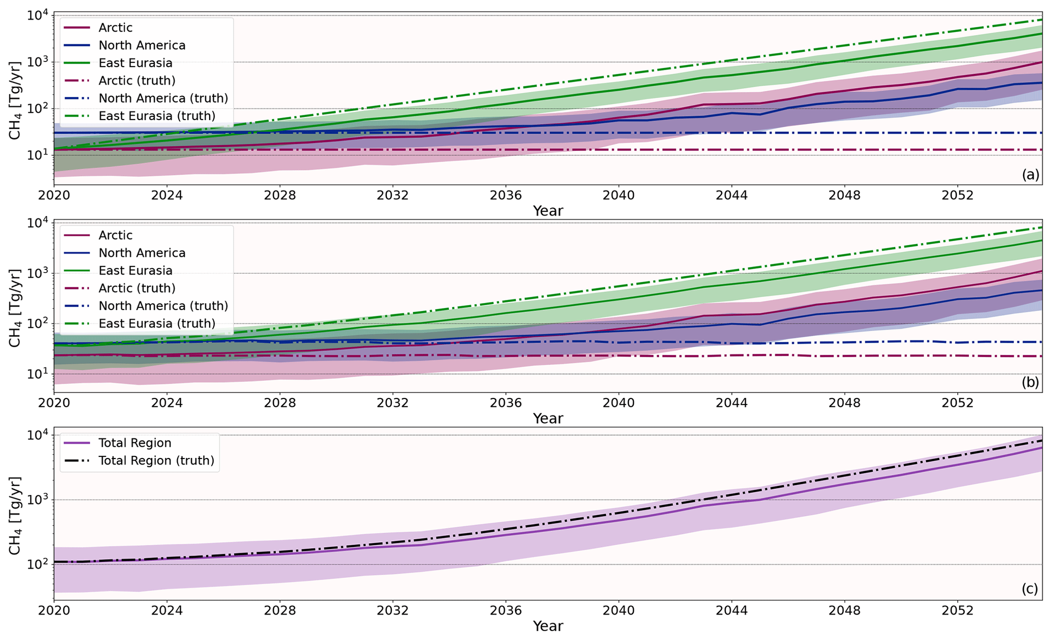
Figure 4Time series of emissions [Tg CH4 yr−1] between 2020 and 2055 with a 20 % yr−1 increase in wetland emissions in East Eurasia. The continuous lines show the posterior state, and the dash-dotted the true state. The Arctic is shown in pink, North America in blue, East Eurasia in green and the entire region in purple. The shaded areas indicate the posterior uncertainties obtained from the Pa matrix. (a) Regional wetland CH4 emissions, (b) regional total CH4 emissions and (c) entire total CH4 emissions.
Since wetland emissions are only increased in East Eurasia in this scenario, only this region should be updated by the inversion. It is shown that the posterior emissions are indeed increasing in this region, however, at a lower rate than intended by the scenario. By the year 2055, the posterior emissions (≈ 4092 Tg CH4 yr−1) are approximately 50 % less than the truth (≈ 8152 Tg CH4 yr−1). This is also found for the total emissions in the entire Arctic and sub-Arctic region, where the posterior emissions are around 28 % less than the truth in 2055.
However, it is shown that the posterior wetland emissions are also increasing over time in regions where no trend was applied, such as North America. Here, the posterior state starts deviating from the truth at around 2032. At the end of the period in 2055, the annual CH4 emissions from wetlands are ≈ 330 Tg higher than the given unmodified truth (≈ 30 Tg CH4 yr−1).
This means that the increase retrieved in the posterior state is underestimated compared to the generated truth in the correct area, which is considered to be the true state of the emissions in this inversion set-up. This is partially compensated for in the total posterior by overestimations in the same emission sector in different regions.
When the same emission scenario (20 % increase in wetland emissions) is applied exclusively to North America, the opposite effect is observed: the posterior emissions in North America are underestimated to be around 26 % less than the truth and in East Eurasia the posterior CH4 fluxes are significantly higher compared to the truth. The discrepancies are, however, lower in comparison to the scenario anticipating elevated wetland emissions in East Eurasia. This can be explained by the denser observation network available in North America, resulting in a better posterior distribution of fluxes. Similar results are obtained under elevated anthropogenic CH4 emissions.
4.2 Regional trend detection
Subsequently, we analyse how well the prescribed trends in the different regions are detected by the inversion in the posterior state. In order to summarise the results of the numerous scenarios, all the figures presented in this section encompass 121 scenarios described in Sect. 3.5: in 120 of these scenarios, the trend was applied on wetland emissions in only one of the corresponding sub-regions, in the remaining scenario the trend was only applied to oceanic CH4 emissions in the ESAS region (see Supplement, Fig. S1d). These scenarios are chosen for the illustration figures since similar results are obtained for anthropogenic CH4 emissions.
4.2.1 Trend detection threshold
We define a temporal threshold in each of the 121 sub-regions r in order to determine when the posterior state is statistically different from the prior.
For this, we select the years for which the difference between the annual posterior emissions in year j and region r emis and the prior emis is larger than the absolute posterior error in the threshold year:
with and .
The threshold year is therefore defined as the first year for which Eq. (4) is not fulfilled.
Due to the looping of footprints and fluxes from 12 years to generate the future truth (described in Sect. 2), the criterion may be matched for some years discontinuously first, then continuously until 2055. The threshold is therefore the first year after which all years are flagged as detected, as illustrated in Fig. 3. As expected, the threshold year is generally later for regions with a sparse observation network (Fig. 5a).
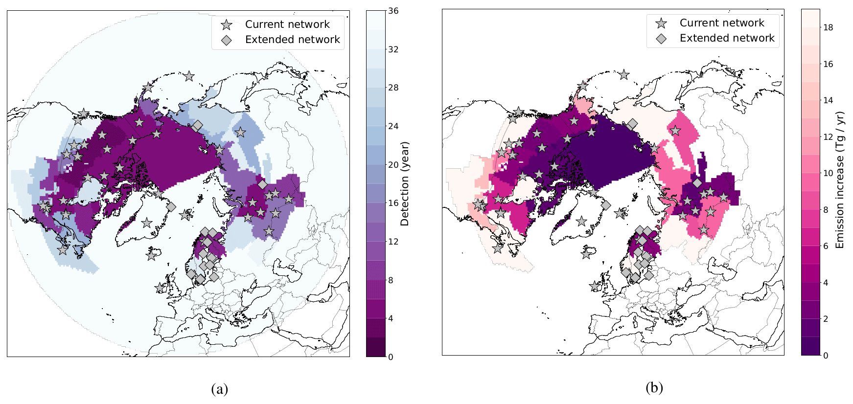
Figure 5(a) Threshold year counted from 2020 for each sub-region. In the ESAS region, the trend applied to ocean emissions is 100 % yr−1; for all other regions, a trend of 20 % yr−1 is applied to wetland emissions. The inversion is performed using the current observation network only (grey stars). The stations of the extended network are indicated by grey diamonds. (b) Increment in yearly emissions for each sub-region at the threshold of detection, in Tg yr−1.
In regions with a dense network, such as northern North America, the threshold year is quite early (after ≈ 5 years of 36). These figures reflect an ideal case where uncertainties in the inversion system are minimised, in particular on the synthetic observations as described in Sect. 2, and it is assumed that data are immediately available. In reality, it could take much longer to detect a significant trend, even in regions with relatively dense networks. Moreover, the applied trend of 20 % yr−1 for wetlands and 100 % yr−1 for ESAS is particularly pessimistic. For example, a trend of +20 % yr−1 for wetlands in East Eurasia results in emissions increasing from less than 14 Tg in 2020 up to 8150 Tg in 2055, totally unrealistic compared to present-day global emissions of 550–880 Tg yr−1 (Saunois et al., 2020).
Hence, it is more illustrative to analyse the smallest quantity of emissions which can be detected, as shown in Fig. 5b, than simply using the year of detection as an indicator. As also observed for the threshold year, the emission threshold is generally smaller near the denser part of the network. In most regions, even in the most favourable parts of the Arctic in terms of detection limits, an increase of a few up to 10 Tg yr−1 (which corresponds to an increase of approximately 7 % yr−1), is necessary for statistically reliable detection. Such detection thresholds are close to the expected emission increases in the coming decades, e.g. 20 Tg yr−1 from thawing permafrost in Siberia (Anisimov and Zimov, 2021). This raises possible limitations in the detection of such events, as the detection limits further away from the observation networks are much higher. More realistic scenarios would take much longer to be detected.
4.2.2 Detection of trend magnitudes
Subsequently, we want to examine how well the previously determined trends of 20 % increase in wetland emissions and 100 % increase in oceanic CH4 emissions are captured in each of the corresponding sub-regions.
Therefore, the relative difference Δemisj,r is the difference between the posterior annual CH4 emissions emis in the threshold year defined in Sect. 4.2.1 and the corresponding truth emis divided by the truth in the threshold year:
for and . Therefore, the closer Δemisj,r is to zero, the better the truth is captured in the posterior state of the corresponding sub-region.
As expected, the posterior increment in the defined threshold year is closer to the truth in areas with a dense observation network (Fig. 6a). These include North America, parts of Siberia, the RECCAP region containing ESAS and parts of northern Europe: the posterior results deviate from the truth by between approximately 0 % and 45 %. The exceptions are some oceanic regions outside the Arctic Ocean. Here, the small differences between the posterior emissions and the truth are unrelated to the observation network but due to the absence of trends.
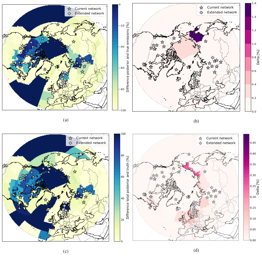
Figure 6(a) Relative difference (%) between posterior and true annual CH4 emissions (Tg CH4 yr−1) in the threshold year of the corresponding region. Darker shading indicate regions where the increment in the posterior state is closer to the truth. The inversion is performed using the extended network. (b) Difference between current and extended observation networks regarding the relative differences between the truth and the posterior state. (c) Relative difference of total CH4 emissions in the pan-Arctic domain and true increment corresponding sub-region. (d) Difference between current and extended observation network regarding the total and true increment.
Additionally, in order to determine the share of the truth detected by the inversion, we calculate the detection ratio Kj,r. Here, the posterior increment in all regions in the threshold year j is divided by the true increment in region r:
with and .
Hence, we analyse how much of the true increase is detected, independent from the location it is attributed to, when increasing the CH4 emissions in one of the sub-regions. Higher values indicate that a larger share of the true emissions is detected in the posterior emission, distributed over the whole pan-Arctic domain. Figure 6c shows that the detection ratio is generally higher when the true emissions are increased in regions with a dense observation network (such as North America), with values of up to 100 %. Similar to the relative difference (Fig. 6a), the high detection ratios in the oceanic regions are due to the absence of trends in the true emissions, since the CH4 emissions in these regions are nearly zero.
When comparing the two observation networks, the improvements achieved by the additional sites are remarkably small: the posterior state of the extended network is closer to the truth by a maximum of 1.6 % in comparison to the current network (Fig. 6b). Regarding the comparison of the detection ratio of the two networks, shown in Fig. 6d, the improvement is even smaller with a maximum of 0.3 %. Only the two added stations at the coast of the East Siberian Sea (AMB and CHS) seem to provide additional constraints for the surrounding regions. One possible reason for this could be related to the locations of the additional observation sites, as several of them are located close to operating measurement stations and/or in areas with low estimated CH4 fluxes.
In northern Europe, where the network was extended by 10 sites, the differences between the current and the extended networks are not significant. This is related to our particular set-up, for which background concentrations are optimised alongside fluxes. In northern Europe, despite the provision of numerous additional sites, the inversion attributes observation discrepancies between the truth and the prior to the background concentrations instead of to the fluxes.
4.2.3 Misattribution of CH4 emissions
The inversion may produce artefacts and detect trends not only in the region where a trend is applied to the truth but also in other regions. To assess this issue, we calculate how much increase is detected in the posterior CH4 emissions in all other regions for the given threshold year in relation to the growth detected in the region in which the increment is actually applied. In other words, we evaluate how much emissions due to the trend in the region examined is misattributed to other regions.
For instance, for an applied trend in RECCAP region i, the posterior increment ratio can be defined as
for the threshold year and the region . and here represent the difference between the posterior CH4 emissions in the threshold year j and the true emissions in the year 2020 in the corresponding region r or i respectively.
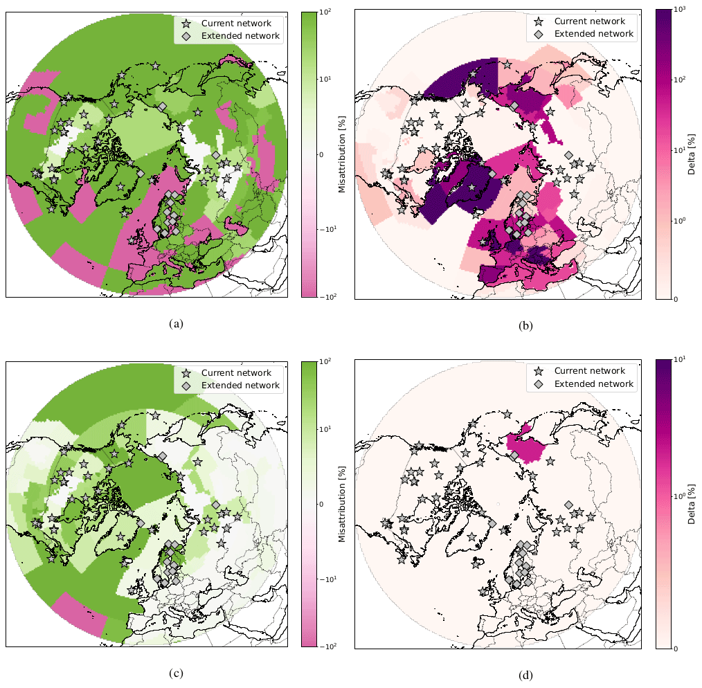
Figure 7(a) Misattribution of detected CH4 emissions to regions other than the region a trend is applied to. Deeper shading shows here a large increase (green) or decrease (pink) in other regions. Areas coloured in deep green show regions for which the increment outside is much larger than inside the region, where the increment was intended; pink coloured regions tend to decrease CH4 fluxes outside. The closer to white the colour of a region, the less the emissions are modified outside of it. (b) Difference between the posterior increment ratio of current and extended network. Darker shades of purple show regions where the extended network performs better in comparison to the current network regarding the misattribution. (c) Misattribution of true CH4 emissions (colours as in panel (a)). (d) Difference of true increment ratio between current and extended observation network.
Areas with a denser observation network generally show less misattribution of CH4 fluxes to other regions (Fig. 7a), following the results presented in Sect. 4.2.2. Here, the posterior increment ratio in other regions is around 0 % to 40 %. For areas with a sparse network of surface observation sites, increases in CH4 fluxes in other regions can be more than 1000 %.
The improvements achieved through the expansion of the network are more substantial regarding the misattribution of CH4 fluxes to other regions (Fig. 7b), compared to the results presented in Sect. 4.2.2. For example, the improvement by the two stations, AMB and CHS, described in the previous section can also be observed here. For the region those sites are located in, the posterior increment ratio was 286 % in the scenario using the current network and only 34 % in the extended network. Improvements are also found in Europe and Greenland.
In addition to the posterior increment ratio, we compute the true increment ratio for each sub-region i:
for the threshold year and the region . is here defined as the difference between the true CH4 fluxes in the threshold year j and the truth in 2020 in the corresponding region i. The closer the value of of a specific region is to zero, the less true emissions are misattributed to other sub-regions. The true increment ratios are shown in Fig. 7c. Similar to the posterior increment ratios, the fluxes are generally less misattributed when the true emissions are increased in continental areas with available observation sites, especially in Siberia and Canada. The improvements from the extended observation network are smaller regarding the true increment ratio (see Fig. 7d) in comparison to the posterior increment ratio, with only one region in eastern Siberia showing a clear improvement of around 10 %.
In this study, we generated numerous future scenarios simulating an assumed methane bomb in high northern latitudes. To determine how well the existing in situ observation network (consisting of 40 sites) and a possible future network (56 sites) are able to detect increases in CH4 emissions, these scenarios were integrated in an analytical inversion framework.
The period under study covers the years 2020 to 2055. During this period, different annual increases are applied to three CH4 sources: wetlands, oceanic sources and anthropogenic emissions. The scenarios of possible trends were applied to different sub-regions in the high northern latitudes. Methane bombs due to particular types of source are not discussed separately here. In fact, it is likely that emissions from these CH4 sources will increase simultaneously as a result of Arctic warming. Therefore, we focus on spatial patterns in order to detect trends.
In this approach, we have made the optimistic assumption of excellent quality and availability of measurement data. The results presented therefore represent the best possible scenario for detecting a future Arctic methane bomb.
The posterior CH4 emissions are underestimated (by up to 41 %) in most regions a trend was assigned to. The discrepancies are larger in later years and proportional to the magnitude of the true trend. Additionally, increasing posterior CH4 fluxes are also found in regions where increasing emissions are not prescribed. This effect is smaller when the true trend is assigned to regions with a dense observation network. However, the additional hypothetical sites bring little improvement in this regard. This indicates that neither of the two observation networks is able to correctly quantify and locate increases in Arctic methane emissions.
For the correct detection of the true trend in a specific area, the regional differences confirm that detection is better in regions with numerous observation sites, such as northern North America or parts of Siberia. Still, the improvements achieved by the extended observation network are remarkably small. A noticeable improvement is only found in the north-east of Russia, and the detection is only up to 1.6 % better than with the current network.
A more significant advantage of the extended observation network is linked to the misattribution of CH4 fluxes. As stated before, the results show that increased CH4 emissions are not only detected in the region where the trend actually occurs but that false positives are detected in other regions. The inversion set-ups using the extended observation network show significant improvements, for instance in the north-east of Russia, in Europe and in Greenland.
Overall, this study shows that methane bombs could be detected in Arctic regions with good observational coverage within 2 to 10 years, while in poorly covered regions detection would take 10 to 30 years, with the added risk of triggering false positives in other regions.
Therefore, efforts to integrate mobile campaigns and new-generation satellite observations into inverse modelling systems should be supported and developed further. Satellite observations in particular offer a high potential to compensate for the lack of in situ observations in the Arctic. The feasibility of using available satellite data products for inverse modelling of methane emissions in high northern latitudes has been discussed, for instance by Berchet et al. (2015), and several approaches integrating these observations in Arctic regions (e.g. TROPOMI CH4 products, Tsuruta et al., 2023) have been implemented. However, the quality of the data provided by currently operating remote sensing instruments is hampered in high northern latitudes by factors such as high solar zenith angles, low albedo of the Arctic Ocean and limited daylight during polar nights. However, new satellite missions (e.g. the Franco-German MERLIN project) will possibly provide large, accurate and high-resolution data sets, suitable for characterising CH4 plumes from regional sources and better constraining methane fluxes in the Arctic.
Current political differences and the associated sanctions are an additional obstacle regarding the accessibility of crucial CH4 observations in the Russian Arctic and sub-Arctic. As the network in this region is already limited, this missing information may further hamper obtaining a complete picture of ongoing processes in the Arctic, including the detection of a possible methane bomb.
The transport model FLEXPART 10.4 is open source, and the source code is freely available on the FLEXPART website at https://www.flexpart.eu/downloads/66 (FLEXPART, 2023). The model is described in detail by Pisso et al. (2019). Flux data were obtained from the Global Carbon Project – Methane (https://www.icos-cp.eu/GCP-CH4/2019, data at Saunois et al., 2020). The contribution of the background concentrations was calculated using the code of the Community Inversion Framework available at https://doi.org/10.5281/zenodo.5045730 (Berchet et al., 2021b).
The supplement related to this article is available online at: https://doi.org/10.5194/acp-24-6359-2024-supplement.
SW designed the analytical inversion system, ran the FLEXPART simulations and performed the scientific analysis presented in the paper. AB and IP provided scientific and technical expertise and contributed to the scientific analysis. MS provided the CH4 fluxes from the Global Carbon Project, and JDP contributed scientific expertise.
The contact author has declared that none of the authors has any competing interests.
Publisher’s note: Copernicus Publications remains neutral with regard to jurisdictional claims made in the text, published maps, institutional affiliations, or any other geographical representation in this paper. While Copernicus Publications makes every effort to include appropriate place names, the final responsibility lies with the authors.
We would like to thank all PIs and supporting staff for deploying, maintaining and making available data from observation sites around the Arctic. In particular, we thank our colleagues from the V. E. Zuev Institute of Atmospheric Optics (Tomsk). We thank the staff supporting the data infrastructure of ICOS (Integrated Carbon Observing System; https://www.icos-cp.eu, last access: 8 October 2023), the WDCGG (World Data Centre for Greenhouse Gases; https://gaw.kishou.go.jp/, last access: 8 October 2023) and ObsPack (https://www.gml.noaa.gov/ccgg/obspack/, last access: 8 October 2023) for distributing observations.
This research has been supported by CEA NUMERICS, funded by the European Union's Horizon 2020 programme under Marie Sklodowska-Curie Actions (grant no. 800945).
This paper was edited by Bryan N. Duncan and reviewed by two anonymous referees.
AMAP: Assessment 2015: Methane as an Arctic climate forcer. Arctic Monitoring and Assessment Programme (AMAP), Oslo, Norway. vii + 139 pp., https://www.amap.no/documents/doc/amap-assessment-2015-methane-as-an-arctic-climate-forcer/1285 (last access: 8 October 2023), 2015. a, b
AMAP: Arctic Climate Change Update 2021: Key Trends and Impacts. Arctic Monitoring and Assessment Programme (AMAP), Tromsø, Norway, viii + 148 pp., https://www.amap.no/documents/doc/arctic-climate-change-update-2021-key-trends-and-impacts.-summary-for-policy-makers/3508 (last access: 8 October 2023), 2021. a, b
Ananthaswamy, A.: The methane apocalypse, New Sci., 226, 38–41, 2015. a
Anisimov, O. and Zimov, S.: Thawing permafrost and methane emission in Siberia: Synthesis of observations, reanalysis, and predictive modeling, Ambio, 50, 2050–2059, 2021. a, b
Arctic-Council: Expert Group on Black Carbon and Methane – Summary of Progress and Recommendations 2019, 88 pp., Arctic Council Secretariat, http://hdl.handle.net/11374/2610 (last access: 8 October 2023), 2019. a
Berchet, A., Pison, I., Chevallier, F., Paris, J.-D., Bousquet, P., Bonne, J.-L., Arshinov, M. Y., Belan, B. D., Cressot, C., Davydov, D. K., Dlugokencky, E. J., Fofonov, A. V., Galanin, A., Lavrič, J., Machida, T., Parker, R., Sasakawa, M., Spahni, R., Stocker, B. D., and Winderlich, J.: Natural and anthropogenic methane fluxes in Eurasia: a mesoscale quantification by generalized atmospheric inversion, Biogeosciences, 12, 5393–5414, https://doi.org/10.5194/bg-12-5393-2015, 2015. a
Berchet, A., Bousquet, P., Pison, I., Locatelli, R., Chevallier, F., Paris, J.-D., Dlugokencky, E. J., Laurila, T., Hatakka, J., Viisanen, Y., Worthy, D. E. J., Nisbet, E., Fisher, R., France, J., Lowry, D., Ivakhov, V., and Hermansen, O.: Atmospheric constraints on the methane emissions from the East Siberian Shelf, Atmos. Chem. Phys., 16, 4147–4157, https://doi.org/10.5194/acp-16-4147-2016, 2016. a
Berchet, A., Sollum, E., Thompson, R. L., Pison, I., Thanwerdas, J., Broquet, G., Chevallier, F., Aalto, T., Berchet, A., Bergamaschi, P., Brunner, D., Engelen, R., Fortems-Cheiney, A., Gerbig, C., Groot Zwaaftink, C. D., Haussaire, J.-M., Henne, S., Houweling, S., Karstens, U., Kutsch, W. L., Luijkx, I. T., Monteil, G., Palmer, P. I., van Peet, J. C. A., Peters, W., Peylin, P., Potier, E., Rödenbeck, C., Saunois, M., Scholze, M., Tsuruta, A., and Zhao, Y.: The Community Inversion Framework v1.0: a unified system for atmospheric inversion studies, Geosci. Model Dev., 14, 5331–5354, https://doi.org/10.5194/gmd-14-5331-2021, 2021a. a
Berchet, A., Sollum, E., Pison, I., Thompson, R. L., Thanwerdas, J., Fortems-Cheiney, A., van Peet, J. C. A., Potier, E., Chevallier, F., Broquet, G., and Berchet, A.: The Community Inversion Framework: codes and documentation, Zenodo [code], https://doi.org/10.5281/zenodo.5045730, 2021b. a
Ciais, P., Bastos, A., Chevallier, F., Lauerwald, R., Poulter, B., Canadell, J. G., Hugelius, G., Jackson, R. B., Jain, A., Jones, M., Kondo, M., Luijkx, I. T., Patra, P. K., Peters, W., Pongratz, J., Petrescu, A. M. R., Piao, S., Qiu, C., Von Randow, C., Regnier, P., Saunois, M., Scholes, R., Shvidenko, A., Tian, H., Yang, H., Wang, X., and Zheng, B.: Definitions and methods to estimate regional land carbon fluxes for the second phase of the REgional Carbon Cycle Assessment and Processes Project (RECCAP-2), Geosci. Model Dev., 15, 1289–1316, https://doi.org/10.5194/gmd-15-1289-2022, 2022. a
Damm, E., Helmke, E., Thoms, S., Schauer, U., Nöthig, E., Bakker, K., and Kiene, R. P.: Methane production in aerobic oligotrophic surface water in the central Arctic Ocean, Biogeosciences, 7, 1099–1108, https://doi.org/10.5194/bg-7-1099-2010, 2010. a
Etiope, G., Ciotoli, G., Schwietzke, S., and Schoell, M.: Gridded maps of geological methane emissions and their isotopic signature, Earth Syst. Sci. Data, 11, 1–22, https://doi.org/10.5194/essd-11-1-2019, 2019. a
FLEXPART: https://www.flexpart.eu/downloads/66, last access: 8 October 2023. a
Gautier, D. L., Bird, K. J., Charpentier, R. R., Grantz, A., Houseknecht, D. W., Klett, T. R., Moore, T. E., Pitman, J. K., Schenk, C. J., Schuenemeyer, J. H., Sorensen, K., Tennyson, M. E., Valin, Z. C., and Wandrey, C. J.: Assessment of undiscovered oil and gas in the arctic, Science, 324, 1175–1179, https://doi.org/10.1126/science.1169467, 2009. a
Glikson, A.: The methane time bomb, Energy Proced., 146, 23–29, 2018. a, b
Hersbach, H., Bell, B., Berrisford, P., Hirahara, S., Horányi, A., Muñoz-Sabater, J., Nicolas, J., Peubey, C., Radu, R., Schepers, D., Simmons,A., Soci, C., Abdalla, S., Abellan, X., Balsamo, G., Bechtold, P., Biavati, G., Bidlot, J., Bonavita, M., De Chiara, G., Dahlgren, P., Dee,D., Diamantakis, M., Dragani, R., Flemming, J., Forbes, R., Fuentes, M., Geer, A., Haimberger, L., Healy, S., Hogan, R. J., Hólm, E.,Janisková, M., Keeley, S., Laloyaux, P., Lopez, P., Lupu, C., Radnoti, G., de Rosnay, P., Rozum, I., Vamborg, F., Villaume, S., and Thépaut,J.-N.: The ERA5 global reanalysis, Q. J. Roy. Meteor. Soc., 146, 1999–2049, https://doi.org/10.1002/qj.3803, 2020. a
Inness, A., Ades, M., Agustí-Panareda, A., Barré, J., Benedictow, A., Blechschmidt, A.-M., Dominguez, J. J., Engelen, R., Eskes, H., Flemming, J., Huijnen, V., Jones, L., Kipling, Z., Massart, S., Parrington, M., Peuch, V.-H., Razinger, M., Remy, S., Schulz, M., and Suttie, M.: The CAMS reanalysis of atmospheric composition, Atmos. Chem. Phys., 19, 3515–3556, https://doi.org/10.5194/acp-19-3515-2019, 2019. a
Klotz, L. A., Sonnentag, O., Wang, Z., Wang, J. A., and Kang, M.: Oil and natural gas wells across the NASA ABoVE domain: fugitive methane emissions and broader environmental impacts, Environ. Res. Lett., 18, 035008, https://doi.org/10.1088/1748-9326/acbe52, 2023. a
Kort, E., Wofsy, S., Daube, B., Diao, M., Elkins, J., Gao, R., Hintsa, E., Hurst, D., Jimenez, R., Moore, F., Spackman, J., and Zondlo, M.: Atmospheric observations of Arctic Ocean methane emissions up to 82 north, Nat. Geosci., 5, 318–321, 2012. a
Kretschmer, K., Biastoch, A., Rüpke, L., and Burwicz, E.: Modeling the fate of methane hydrates under global warming, Global Biogeochem. Cy., 29, 610–625, 2015. a
Mascarelli, A.: A sleeping giant?, Nature climate change, 1, 46–49, 2009. a
McGuire, A. D., Lawrence, D. M., Koven, C., Clein, J. S., Burke, E., Chen, G., Jafarov, E., MacDougall, A. H., Marchenko, S., Nicolsky, D., Peng, S., Rinke, A., Ciais, P., Gouttevin, I., Hayes, D. J., Ji, D., Krinner, G., Moore, J. C., Romanovsky, V., Schädel, C., Schaefer, K.,Schuur, E. A. G., and Zhuang, Q.: Dependence of the evolution of carbon dynamics in the northern permafrost region on the trajectory of climate change, P. Natl. Acad. Sci. USA, 115, 3882–3887, 2018. a
Pisso, I., Sollum, E., Grythe, H., Kristiansen, N. I., Cassiani, M., Eckhardt, S., Arnold, D., Morton, D., Thompson, R. L., Groot Zwaaftink, C. D., Evangeliou, N., Sodemann, H., Haimberger, L., Henne, S., Brunner, D., Burkhart, J. F., Fouilloux, A., Brioude, J., Philipp, A., Seibert, P., and Stohl, A.: The Lagrangian particle dispersion model FLEXPART version 10.4, Geosci. Model Dev., 12, 4955–4997, https://doi.org/10.5194/gmd-12-4955-2019, 2019. a, b, c
Poulter, B., Bousquet, P., Canadell, J. G., Ciais, P., Peregon, A., Saunois, M., Arora, V. K., Beerling, D. J., Brovkin, V., Jones, C. D.,Joos, F., Gedney, N., Ito, A., Kleinen, T., Koven, C. D., McDonald, K., Melton, J. R., Peng, C., Peng, S., Prigent, C., Schroeder, R.,Riley, W. J., Saito, M., Spahni, R., Tian, H., Taylor, L., Viovy, N., Wilton, D., Wiltshire, A., Xu, X., Zhang, B., Zhang, Z., and Zhu, Q.: Global wetland contribution to 2000–2012 atmospheric methane growth rate dynamics, Environ. Res. Lett., 12, 094013, https://doi.org/10.1088/1748-9326/aa8391, 2017. a
Rantanen, M., Karpechko, A. Y., Lipponen, A., Nordling, K., Hyvärinen, O., Ruosteenoja, K., Vihma, T., and Laaksonen, A.: The Arctic has warmed nearly four times faster than the globe since 1979, Commun. Earth Environ., 3, 168 https://doi.org/10.1038/s43247-022-00498-3, 2022. a
Ridgwell, A. J., Marshall, S. J., and Gregson, K.: Consumption of atmospheric methane by soils: A process-based model, Global Biogeochem. Cy., 13, 59–70, https://doi.org/10.1029/1998GB900004, 1999. a
Saunois, M., Stavert, A. R., Poulter, B., Bousquet, P., Canadell, J. G., Jackson, R. B., Raymond, P. A., Dlugokencky, E. J., Houweling, S., Patra, P. K., Ciais, P., Arora, V. K., Bastviken, D., Bergamaschi, P., Blake, D. R., Brailsford, G., Bruhwiler, L., Carlson, K. M., Carrol, M., Castaldi, S., Chandra, N., Crevoisier, C., Crill, P. M., Covey, K., Curry, C. L., Etiope, G., Frankenberg, C., Gedney, N., Hegglin, M. I., Höglund-Isaksson, L., Hugelius, G., Ishizawa, M., Ito, A., Janssens-Maenhout, G., Jensen, K. M., Joos, F., Kleinen, T., Krummel, P. B., Langenfelds, R. L., Laruelle, G. G., Liu, L., Machida, T., Maksyutov, S., McDonald, K. C., McNorton, J., Miller, P. A., Melton, J. R., Morino, I., Müller, J., Murguia-Flores, F., Naik, V., Niwa, Y., Noce, S., O'Doherty, S., Parker, R. J., Peng, C., Peng, S., Peters, G. P., Prigent, C., Prinn, R., Ramonet, M., Regnier, P., Riley, W. J., Rosentreter, J. A., Segers, A., Simpson, I. J., Shi, H., Smith, S. J., Steele, L. P., Thornton, B. F., Tian, H., Tohjima, Y., Tubiello, F. N., Tsuruta, A., Viovy, N., Voulgarakis, A., Weber, T. S., van Weele, M., van der Werf, G. R., Weiss, R. F., Worthy, D., Wunch, D., Yin, Y., Yoshida, Y., Zhang, W., Zhang, Z., Zhao, Y., Zheng, B., Zhu, Q., Zhu, Q., and Zhuang, Q.: The Global Methane Budget 2000–2017, Earth Syst. Sci. Data, 12, 1561–1623, https://doi.org/10.5194/essd-12-1561-2020, 2020 (data available at: https://www.icos-cp.eu/GCP-CH4/2019, last access: 8 October 2023). a, b, c, d, e
Schneider von Deimling, T., Grosse, G., Strauss, J., Schirrmeister, L., Morgenstern, A., Schaphoff, S., Meinshausen, M., and Boike, J.: Observation-based modelling of permafrost carbon fluxes with accounting for deep carbon deposits and thermokarst activity, Biogeosciences, 12, 3469–3488, https://doi.org/10.5194/bg-12-3469-2015, 2015. a
Schuur, E., McGuire, A., Schädel, C., Grosse, G., Harden, J., Hayes, D., Hugelius, G., Koven, C., Kuhry, P., Lawrence, D., Natali, S., Olefeldt, D., Romanovsky, V., Schaefer, K., Turetsky, M., Treat, C., and Vonk, J.: Climate change and the permafrost carbon feedback, Nature 520, 171–179, https://doi.org/10.1038/nature14338, 2015. a
Schuur, E. A., Abbott, B. W., Commane, R., Ernakovich, J., Euskirchen, E., Hugelius, G., Grosse, G., Jones, M., Koven, C., Leshyk, V., Lawrence, D., Loranty, M. M., Mauritz, M., Olefeldt, D., Natali, S., Rodenhizer, H., Salmon, V., Schädel, C., Strauss, J., Treat, C., and Turetsky, M.: Permafrost and Climate Change: Carbon Cycle Feedbacks from the Warming Arctic, Annu. Rev. Env. Resour., 47, 343–371, 2022. a
Seibert, P. and Frank, A.: Source-receptor matrix calculation with a Lagrangian particle dispersion model in backward mode, Atmos. Chem. Phys., 4, 51–63, https://doi.org/10.5194/acp-4-51-2004, 2004. a
Shakhova, N., Alekseev, V., and Semiletov, I.: Predicted methane emission on the East Siberian shelf, in: Doklady Earth Sciences, vol. 430, p. 190, Springer Nature BV, https://doi.org/10.1134/S1028334X10020091, 2010. a
Shakhova, N., Semiletov, I., Sergienko, V., Lobkovsky, L., Yusupov, V., Salyuk, A., Salomatin, A., Chernykh, D., Kosmach, D., Panteleev,G., Nicolsky, D., Samarkin, V., Joye, S., Charkin, A., Dudarev, O., Meluzov, A., and Gustafsson, O.: The East Siberian Arctic Shelf: towards further assessment of permafrost-related methane fluxes and role of sea ice, Philos. T. Roy. Soc. A, 373, 20140451, https://doi.org/10.1098/rsta.2014.0451, 2015. a
Shakhova, N., Semiletov, I., and Chuvilin, E.: Understanding the permafrost–hydrate system and associated methane releases in the East Siberian Arctic shelf, Geosciences, 9, 251, https://doi.org/10.3390/geosciences9060251, 2019. a
Stohl, A., Forster, C., Frank, A., Seibert, P., and Wotawa, G.: Technical note: The Lagrangian particle dispersion model FLEXPART version 6.2, Atmos. Chem. Phys., 5, 2461–2474, https://doi.org/10.5194/acp-5-2461-2005, 2005. a
Szénási, B., Berchet, A., Broquet, G., Segers, A., Denier van der Gon, H., Krol, M., Hullegie, J. J., Kiesow, A., Günther, D., Petrescu, A. M. R., Saunois, M., Bousquet, P., and Pison, I.: A pragmatic protocol for characterising errors in atmospheric inversions of methane emissions over Europe, Tellus B, 73, 1–23, 2021. a
Thompson, R. L. and Stohl, A.: FLEXINVERT: an atmospheric Bayesian inversion framework for determining surface fluxes of trace species using an optimized grid, Geosci. Model Dev., 7, 2223–2242, https://doi.org/10.5194/gmd-7-2223-2014, 2014. a
Tipka, A., Haimberger, L., and Seibert, P.: Flex_extract v7.1.2 – a software package to retrieve and prepare ECMWF data for use in FLEXPART, Geosci. Model Dev., 13, 5277–5310, https://doi.org/10.5194/gmd-13-5277-2020, 2020.
Treat, C. C., Natali, S. M., Ernakovich, J., Iversen, C. M., Lupascu, M., McGuire, A. D., Norby, R. J., Roy Chowdhury, T., Richter, A., Santruckova, H., Schädel, C., Schuur, E. A. G., Sloan, V. L., Turetsky, M. R., and Waldrop, M. P.: A pan-Arctic synthesis of potential CH4 and CO2 production from anoxic soil incubations, Glob. Change Biol., 13, 1922–1934, https://doi.org/10.1111/gcb.12875, 2015. a
Tsuruta, A., Kivimäki, E., Lindqvist, H., Karppinen, T., Backman, L., Hakkarainen, J., Schneising, O., Buchwitz, M., Lan, X., Kivi, R., Chen, H., Buschmann, M., Herkommer, B., Notholt, J., Roehl, C., Té, Y., Wunch, D., Tamminen, J., and Aalto, T.: CH4 Fluxes Derived from Assimilation of TROPOMI XCH4 in CarbonTracker Europe-CH4: Evaluation of Seasonality and Spatial Distribution in the Northern High Latitudes, Remote Sensing, 15, 1620, https://doi.org/10.3390/rs15061620, 2023. a
Walter Anthony, K., Schneider von Deimling, T., Nitze, I., Frolking, S., Emond, A., Daanen, R., Anthony, P., Lindgren, P., Jones, B., and Grosse, G.: 21st-century modeled permafrost carbon emissions accelerated by abrupt thaw beneath lakes, Nat. Commun., 9, 1–11, 2018. a
Weber, T., Wiseman, N. A., and Kock, A.: Global ocean methane emissions dominated by shallow coastal waters, Nat. Commun., 10, 4584, https://doi.org/10.1038/s41467-019-12541-7, 2019. a
Whiteman, G., Hope, C., and Wadhams, P.: Vast costs of Arctic change, Nature, 499, 401–403, 2013. a
Wild, B., Shakhova, N., Dudarev, O., Ruban, A., Kosmach, D., Tumskoy, V., Tesi, T., Joß, H., Alexanderson, H., Jakobsson, M., Mazurov, A., Semiletov, I., and Gustafsson, Ö.: Organic matter across subsea permafrost thaw horizons on the East Siberian Arctic Shelf, The Cryosphere Discuss. [preprint], https://doi.org/10.5194/tc-2018-229, 2018. a
Wittig, S., Berchet, A., Pison, I., Saunois, M., Thanwerdas, J., Martinez, A., Paris, J.-D., Machida, T., Sasakawa, M., Worthy, D. E. J., Lan, X., Thompson, R. L., Sollum, E., and Arshinov, M.: Estimating methane emissions in the Arctic nations using surface observations from 2008 to 2019, Atmos. Chem. Phys., 23, 6457–6485, https://doi.org/10.5194/acp-23-6457-2023, 2023. a, b, c, d