The impact of multi-decadal changes in VOC speciation on urban ozone chemistry: a case study in Birmingham, United Kingdom

Anthropogenic non-methane volatile organic compounds (VOCs) in the United Kingdom have been substantially reduced since 1990, which is, in part, attributed to controls on evaporative and vehicle tailpipe emissions. Over time, other sources with a different speciation (for example, alcohols from solvent use and industry processes) have grown in both relative importance and, in some cases, in absolute terms. The impact of this change in speciation and the resulting photochemical reactivities of VOCs are evaluated using a photochemical box model constrained by observational data during a summertime ozone event (Birmingham, UK) and apportionment of sources based on the UK National Atmospheric Emission Inventory (NAEI) data over the period 1990–2019. Despite road transport sources representing only 3.3 % of UK VOC emissions in 2019, road transport continued being the sector with the largest influence on the local O₃ production rate (P(O₃)). Under case study conditions, the 96 % reduction in road transport VOC emissions that has been achieved between 1990 and 2019 has likely reduced daytime P(O₃) by ∼ 1.67 ppbv h⁻¹. Further abatement of fuel fugitive emissions was modeled to have had less impact on P(O₃) reduction than abatement of VOCs from industrial processes and solvent use. The long-term trend of increased emissions of ethanol and methanol has somewhat weakened the benefits of reducing road transport emissions, increasing P(O₃) by ∼ 0.19 ppbv h⁻¹ in the case study. Abatement of VOC emissions from multiple sources has been a notable technical and policy success in the UK, but some future benefits (from an ozone perspective) of the phase-out of internal combustion engine passenger cars may be offset if domestic and commercial solvent use of VOCs continue to increase.

1 Introduction

Elevated tropospheric ozone (O₃) has been a long-standing pollutant of concern in the rural and sub-urban environments and is now becoming more prevalent in urban centers, as primary NO traffic emissions decline (Sicard, 2021). As an important tropospheric oxidant and greenhouse gas (Kumar et al., 2021), exposure to O₃ also increases risks of mortality from respiratory diseases and adversely impacts on crop productivity (Lefohn et al., 2018). O₃ is mainly formed through photochemical reactions involving the oxidation of volatile organic compounds (VOCs) in the presence of nitrogen oxides (NO_x; NO_x= NO + NO₂) (Calvert et al., 2015). The release of VOCs arises from a wide range of activities, including unburned fuel or partially combusted products in exhausts from solvents used in the industry and numerous other diffuse domestic and commercial sources (He et al., 2019). Effective policies to mitigate ozone pollution rely on an accurate estimate of both emissions and speciation of O₃ precursors.

The challenge in reducing O₃ lies in its non-linear relationship with its precursors since individual VOCs have unique capacities for forming ozone. Decades of modeling studies have established regimes where reductions in NO_x or VOC emissions would be preferentially beneficial for mitigating O₃ – i.e., the so-called NO_x-limited or VOC-limited regimes (Seinfeld and Pandis, 2016). Abatement of VOC sources is important in VOC-limited areas since decreasing the emissions can effectively reduce the local O₃ production rate and help limit O₃ peak concentrations (Gaudel et al., 2020). The wide range of sources, including many that are diffuse and occur indoors, and differing photochemical reactivities further complicate O₃ reduction strategies. Different mixes of sources and speciation can lead to a need for localized policies. For example, short-chain alkanes and alkenes with high hydroxyl radical reactivity emitted from on-road transportation in China, have been reported as being responsible for 26 % of national O₃ formation (Wu and Xie, 2017). A field observation study in Delhi, India, reported that the O₃ production in that city was most sensitive to monoaromatics, followed by monoterpenes and alkenes during a post-monsoon period in 2018 (Nelson et al., 2021). Another study at urban sites in Seoul, South Korea, concluded that the O₃ production was controlled by C > 6 aromatics and isoprene during a summer O₃ episode in 2016 (Schroeder et al., 2020). There is, therefore, no one-size-fits-all policy in terms of which sources and sectors to target for optimal O₃ abatement efforts.

Policy and regulation aimed at improving air quality in many countries including the United States, the United Kingdom, and Europe have led to decades of falling VOC emissions (Lewis et al., 2020; Coggon et al., 2021). This reduction can be largely attributed to the successful implementation of tailpipe exhaust aftertreatment technology for gasoline vehicles, effective controls over evaporative emissions from vehicles including re-fueling, and a more widespread set of efforts on mitigating industrial emissions (Winkler et al., 2018). Despite these successes, O₃ remains a pollutant of concern; whilst peak concentrations during O₃ events have reduced in the UK, increases in the long-term urban background O₃ concentrations have been observed since the 1990s (Department for Environment, Food and Rural Affairs, 2023). A variety of explanations have been given to account for the increase, including rising Northern Hemisphere background O₃ and increasing methane, which both contribute to global radiative forcing and enhance the O₃ production (Tarasick et al., 2019; Abernethy et al., 2021); an increase in non-vehicular sources of VOC emissions (McDonald et al., 2018; Yeoman and Lewis, 2021); and a reduction in NO_x in VOC-limited urban areas, leading to greater O₃ production efficiency (Sicard et al., 2020).

The UK National Atmospheric Emissions Inventory (NAEI) for VOCs has shown increases in the relative contribution of solvent usage and the food and wine industry to total national VOC emissions over 1990–2019 and steady growth in the relative importance of oxygenated volatile organic compounds (OVOCs) within the overall speciation (Lewis et al., 2020). In North America and European cities, OVOCs emitted from volatile chemical products (VCPs) can outweigh fossil fuel sources for urban VOCs. Modeling results showed that the additional OVOCs from VCP emissions were the most important species for urban O₃ production, increasing the daily maximum O₃ mixing ratio by as much as 10 ppbv in Los Angeles (Qin et al., 2021). Substantial OVOC emissions can come from unexpected places. For example, alcohols emitted by the use of windshield fluid are now estimated to be a larger VOC source in road transport than tailpipes in the UK (Cliff et al., 2023). From the perspective of O₃ pollution, the benefit of substantial reductions in vehicle emissions, whilst there has been a parallel increasing role of non-industrial solvent usage remains unclear. What effect this shift in speciation has on ozone chemistry is less well studied. One challenge has been the lack of routine measurement of OVOCs in most national air quality monitoring networks (Lewis et al., 2021).

Recent model analyses of decadal trends in ozone centered on the association between extreme weather and ozone events and projected changes in ozone concentration under chemical regime change scenarios. A significant decline in the UK experiencing ozone episodes and an increase in background ozone concentration were found for the past 3 decades (Diaz et al., 2020). Elevated ozone mostly occurs in late spring and summer during anticyclonic conditions, when slow-moving air masses from continental Europe contribute to the accumulation of precursor emissions and enhance the photochemical production of ozone (Hertig et al., 2020; Lewis et al., 2021). Higher temperatures in late summer increase biogenic VOC emissions and reduce ozone deposition, leading to summertime maximum concentrations (Finch and Palmer, 2020). Several studies pointed out that an increasingly hot summer, due to climate change, may offset gains made in the reduction in ozone events over time (Gouldsbrough et al., 2022; Z. Liu et al., 2022). In terms of ozone production sensitivity, reductions in NO emissions have led to a decreasing trend in the annual average concentration. However, 20 % or 40 % NO_x emission reductions would lead to increases in average and maximum ozone concentrations in the UK, with respect to 2018 (Gouldsbrough et al., 2024). In addition to results on NO_x and VOCs sensitivities, Ivatt et al. (2022) revealed that ozone concentrations in North America and Europe were inhibited by aerosol in the 1970s, and this aerosol-inhibited regime has shifted to Asia by 2014.

There have been several recent studies focused on evaluating the impacts of reductions in anthropogenic sources on ozone production. By integrating the US Fuel-based Inventory of Vehicle Emissions (FIVE) into an air quality model, McDonald et al. (2018) assessed ozone sensitivity to mobile-source NO_x emissions over the eastern US, and Coggon et al. (2021) employed FIVE with volatile chemical products (VCPs) to evaluate contributions of VOCs from fossil fuels and different types of VCP emissions to ozone production at an urban background site in New York City. Nelson et al. (2021) used emission inventories from the Emission Database for Global Atmospheric Research (EDGAR) to investigate in situ ozone production sensitivity to five inventory source sectors at an urban site in Delhi. Kang et al. (2022) applied two emission inventories in an air quality model to evaluate the contributions of the industry, road transport, power plants, and biogenic emissions to ozone production in Chinese cities. Although great efforts have been made toward identifying crucial VOC sources in regional ozone production, an understanding of their roles in urban ozone chemistry in the context of historical changes is still lacking.

In this study, we evaluate the effects of changing speciation on urban ozone chemistry using recent field measurements of O₃ and its key precursors such as NO_x, CO, speciated VOCs, and OVOCs in Birmingham, UK, during August 2022. We combine this with changing speciation and relative amounts of VOCs based on long-term trends in the NAEI. The sensitivity of in situ production and OH reactivities of the measured O₃ precursors are investigated by constraining the observational data sets to a zero-dimensional chemical box model. By incorporating the detailed NAEI VOC emission inventories over the period of 1990–2019 into the model, O₃ formation in Birmingham is used as a case study to quantify the impacts of the real-world changes in VOC sources on the urban O₃ production rate. The relative importance of different VOC functional group classes to O₃ production is also evaluated. The results help understand the impacts of decades of abating different VOC-emitting sectors on urban O₃ production and outline the implications for future O₃ control strategies.

2 Materials and methods

2.1 Field observations

The observations are taken from the Birmingham NERC air quality supersite during August 2022. This site is located on the University of Birmingham campus (52°27^′20.2^′′ N, 1°55^′44.3^′′ W). The site has been in operation for many years and represents an urban background environment. It is influenced by transport emissions from nearby arterial roads and residential emissions from the surrounding area. There are no significant industrial activities within a 4 km radius of the site.

Continuous measurements of NO; NO₂; CO; CH₄; VOCs; and O₃; as well as meteorological parameters including air temperature and pressure, relative humidity, wind speed, and direction were made. Briefly, NO and NO₂ were measured by a chemiluminescence-based T200 analyzer (Teledyne API, USA) and the T500U cavity attenuated phase shift (CAPS) analyzer (Teledyne API, USA). The concentration of NO_x was then the statistical sum of NO and NO₂. The mixing ratio of CO was measured by a laser absorption spectroscopy multi-species continuous emissions monitoring instrument (Enviro Technology Service Ltd., UK) (Li et al., 2020). Manual calibration and span checks for the above instruments were performed every 3 d, and automatic zero calibration was set to be performed on a daily basis. O₃ was measured by an O₃ analyzer (Model 49i; Thermo Fisher Scientific Inc., USA) with a minimum detection limit (MDL) of 1.0 ppbv. Meteorological parameters, including air temperature and pressure and relative humidity, were obtained by a weather station (WS300-UMB; Luff GmbH, Germany). Additionally, wind speed and direction were measured by a three-axis ultrasonic anemometer (Gill Instruments Ltd., UK) throughout the campaign.

A gas chromatography–flame ionization detection (GC-FID) analysis system (7890A; Agilent Technologies, USA) was used to quantify 38 individual VOC species. Details on instrument settings and quality assurance/quality control methods can be found in Warburton et al. (2023). In brief, the GC-FID system utilizes dual detectors: one detector for C₂–C₆ non-methane hydrocarbons (NMHCs) and the other detector for the remaining C ≥ 7 hydrocarbons and polar species such as ethers, ketones, and alcohols. Ambient samples were dried at −40 °C using a water trap and then preconcentrated on a carbon adsorbent at the lowest temperature the unit could achieve, which was always lower than −115 °C. Once a 0.5 L sample had been collected, a pre-concentration trap was warmed slightly to −80 °C to purge trapped atmospheric CO₂. The trap was then heated to 190 °C for 3 min, with a counter flow of helium thermally desorbing the concentrated VOCs onto a focusing micro-trap held at a temperature lower than −115 °C. The analytes were flash-heated and passed onto a VF-WAX column. The unresolved analytes (C₂–C₆ NMHCs) were then transferred into a Na₂SO₄-deactivated Al₂O₃ porous-layer open-tubular (PLOT) column via a Deans switch for separation and detection by the first FID. The Dean switch then diverted the analytes onto a fused silica internal diameter to balance column flows and subsequently transfer the VF-WAX column-resolved species into the second FID. Generally, the quantification of C₂–C₆ hydrocarbons was completed by the first FID using 4 ppbv gas standard cylinders (National Physical Laboratory, Teddington, UK). The quantification of C ≥ 7 hydrocarbons and OVOCs was completed by the second FID using an effective carbon number (ECN) with reference to toluene. In this study, the concentration of total VOCs (TVOCs) was defined as the statistical sum of the concentrations of measured individual species, but this is not meant to infer that this represents the total reactive carbon in air, which would always be greater than this value due to unmeasured species. Later in this study, we broadly group species according to their chemical function groups, summing them into alcohols, ketones, alkanes, alkenes, aromatics, aldehydes, and alkynes.

GC-FID system responses were regularly checked by running direct calibration sequences using 4 ppbv gas standard cylinders. It was verified that there was no FID response drift over the analysis period for this study. Additionally, carbon-wise FID responses for all reported species were calculated to verify the use of ECN as a quantification method. Table S1 lists which species were directly calibrated and which used equivalent carbon numbers for quantification. Table S2 shows effective carbon numbers of species which used carbon-wise responses.

2.2 National emission inventory for VOCs

Estimates of UK anthropogenic VOC emissions are taken from the NAEI. The NAEI uses a combination of UK-specific methods and default methods as recommended by the European Monitoring and Evaluation Programme (EMEP)/European Environment Agency (EEA) emission inventory guidebook (European Environment Agency, 2016). Further details can be found in NAEI (2021). The VOC inventory is also disaggregated into inventories for each individual VOC species, and details of the speciation process and assumptions can be found in Lewis et al. (2020).

Methods to estimate emissions can be divided into two groups: those using emission factors and those using point source emissions data reported to regulators by the operators of individual industrial sites. The emission factor methods require UK activity data – for example, the consumption of paint, consumption of a fuel, production of steel, or vehicle kilometers traveled. The activity data are then combined with an emission factor, which expresses the total VOC emission that is expected per unit of a given activity. Most total VOC emission factors are taken from the internationally applied EMEP/EEA emission inventory guidebook and so are not necessarily UK-specific. The factors for road transport are directly calculated for the UK, and a particularly detailed approach is used to estimate emissions using emission factors from the Guidebook for many different vehicle types and emission standards, fuels, and road types combined with detailed transport activity from the UK Department for Transport. Government statistics cannot always provide the necessary activity data for other sectors, so industry data are used instead. For instance, NAEI data on the consumption of products containing organic solvents are from industry sources. The alternative point source method can be used for source categories where emissions data can be obtained for all sites within the sector, and this limits the method to source categories such as crude oil refining, steel production, and chemical production. The emissions data reported by the operators of these sites can be based on emissions monitoring although this is not always the case and emissions might instead be estimated, for example, using emission factors.

The NAEI produces updates to the inventory for total VOC mass emissions by source sector each year to achieve a consistent historic time series reflecting trends in UK emissions. Emissions of individual VOC species are estimated using source-specific speciation profiles, which show the mass fraction of each species or, in some cases, groups of species emitted by the source (NAEI, 2021; Passant, 2002). Over 600 individual VOC species or species groups are included in the speciation based on sources in industry, regulators, and, in some cases, literature sources and databases such as the US EPA SPECIATE database. The speciated inventory tends to be more uncertain than the estimation of the total mass of VOC emissions. The inventory for total VOC mass is updated annually, whereas the speciation profiles are only periodically updated when new information becomes available. Thus, trends in a particular species for a sector are a reflection of changes in total VOC emissions for the sector and do not normally reflect any changes over time in the speciation profile of the sector which may have occurred.

2.3 Photochemical box model

The framework for evaluating effects of changing VOC speciation is a zero-dimensional atmospheric modeling chemistry box model (Wolfe et al., 2016) driven by version 3.3.1 of the Master Chemical Mechanism (MCM v3.3.1) (Saunders et al., 2003; Jenkin et al., 2003). The model can be effective in identifying the instantaneous in situ O₃ sensitivity to changes in individual VOCs. The measured concentrations of 38 VOC species, NO_x, and CO, along with air temperature and pressure and relative humidity, were averaged to a time resolution of 1 h to constrain the model. A 3 d model spin-up, with each 24 h model run constrained by the observational data, was performed in order to initialize the unmeasured compounds and transient radicals. The modeled outputs on the fourth day were taken to represent the steady state of the photochemistry.

Photolysis rates were calculated as a function of the solar zenith angle (Saunders et al., 2003):

$$\begin{array}{}\text{(1)}& J=l{\left(\cos \mathit{\chi }\right)}^m\exp \left(-n\sec \mathit{\chi }\right),\end{array}$$

where J is the photolysis rate in s⁻¹; l, m, and n are constants derived from radiative transfer model runs for clear-sky conditions at an altitude of 0.5 km and literature cross sections/quantum yields; and χ is the solar zenith angle in radians.

The net production rate of O₃ (P(O₃)) is calculated as the difference in the production rate of O₃ and the destruction rate of O₃, as in Eq. (2):

$$\begin{array}{}\text{(2)}& \begin{array}{rl}\mathrm{P}\left({\mathrm{O}}_{\mathrm{3}}\right)& =\left(k_{{\mathrm{HO}}_{\mathrm{2}}+\mathrm{NO}}\left[{\mathrm{HO}}_{\mathrm{2}}\right]\left[\mathrm{NO}\right]+\sum _i{k}_{{\mathrm{RO}}_{{\mathrm{2}}_i}+\mathrm{NO}}\left[{\mathrm{RO}}_{\mathrm{2}}\right]\left[\mathrm{NO}\right]\right)\\ & -(k_{{\mathrm{O}}^{\mathrm{1}}D+{\mathrm{H}}_{\mathrm{2}}\mathrm{O}}\left[{\mathrm{O}}^{\mathrm{1}}D\right]\left[{\mathrm{H}}_{\mathrm{2}}\mathrm{O}\right]+k_{{\mathrm{O}}_{\mathrm{3}}+\mathrm{OH}}\left[{\mathrm{O}}_{\mathrm{3}}\right]\left[\mathrm{OH}\right]\\ & +k_{{\mathrm{O}}_{\mathrm{3}}+{\mathrm{HO}}_{\mathrm{2}}}\left[{\mathrm{O}}_{\mathrm{3}}\right]\left[{\mathrm{HO}}_{\mathrm{2}}\right]k_{{\mathrm{NO}}_{\mathrm{2}}+\mathrm{OH}}\left[{\mathrm{NO}}_{\mathrm{2}}\right]\left[\mathrm{OH}\right]\\ & +\sum _i{k}_{{\mathrm{RO}}_{{\mathrm{2}}_i}+{\mathrm{NO}}_{\mathrm{2}}}\left[{\mathrm{RO}}_{\mathrm{2}}\right]\left[{\mathrm{NO}}_{\mathrm{2}}\right]),\end{array}\end{array}$$

where the former part is the rate of O₃ production, represented by the rate of NO oxidation by HO₂ and RO₂ radicals, and the latter part is the destruction rate of O₃, calculated by the sum of the rate of O₃ photolysis, the rates of the reactions with OH and HO₂ radicals, and the rates of NO₂ loss through reactions with OH and RO₂ radicals.

The sensitivity of O₃ to its precursors is quantified by the index of relative incremental reactivity (RIR) (T. Liu et al., 2022), as in Eq. (3):

$$\begin{array}{}\text{(3)}& \mathrm{RIR}={\displaystyle \frac{\mathrm{\Delta }\mathrm{P}\left({\mathrm{O}}_{\mathrm{3}}\right)}{\mathrm{P}\left({\mathrm{O}}_{\mathrm{3}}\right)}}\times a^{-\mathrm{1}},\end{array}$$

where RIR is the relative incremental reactivity (in % / %), ΔP(O₃) $/$ P(O₃) is the ratio of the change in the O₃ production rate to the base O₃ production rate, and a is the reduction percentage in the input concentration of O₃ precursors – a factor that allows for the effects of changing absolute amounts of VOCs to be evaluated. Here, a value of 30 % was adopted for a.

3 Results and discussion

3.1 Observation overview

The time series of O₃ and its precursors during August 2022 are shown in Fig. 1, subdivided into periods that will be referred to as the initial period, O₃ period, and clear-out period. The three periods covered 1–21 August 2022. Each period included one full week to avoid weekday/weekend differences in NO_x and VOC concentrations impacting differently when O₃ production is compared between the three periods (de Foy et al., 2020). Ozone showed a generally increasing trend from 1 to 14 August and then returned to relatively low concentrations after 15 August 2022. The daily maximum 8 h average O₃ concentrations (MDA8h O₃) during the O₃ period exceeded the WHO guideline value (100 µg m⁻³), ranging from 111 to 153 µg m⁻³. The elevated O₃ during the middle of the month corresponded to more intense photochemical formation under hot weather conditions (32.7 °C in maximum) and higher concentrations of O₃ precursors (Table S3).

The diurnal profile of NO and NO₂ in the three periods generally showed a bimodal pattern, albeit less pronounced in the initial and clear-out periods (Fig. 2). The two peaks likely arise as a consequence of increased traffic volumes at the start and end of the day coupled with boundary layer height changes in the early morning and into the evening (Lee et al., 2020). The average concentrations of NO₂ during 05:00–10:00 UTC+1 were 10.8 ppbv in the O₃ period, which was considerably higher than the concentration of 3.9 ppbv in the initial period and 3.4 ppbv in the clear-out period. The low level of NO in the O₃ period highlights the rapid consumption of NO via photochemical processes. The oxidation of CO is an important source of HO₂ in the atmosphere (Chen et al., 2020), which is in the range of 82.5 to 134.2 ppbv here, with little difference between periods. The diurnal profiles of O₃ peaked at 15:00, with maximum hourly concentrations of 31.6, 67.2, and 30.4 ppbv in the initial, O₃, and clear-out periods, respectively. Slight decreases in O₃ were observed during the nighttime (00:00–05:00 UTC+1), indicating enhanced NO titration effects.

The detailed VOC composition in the three periods is presented in Fig. S1. Concentrations of TVOCs were 19.4 ± 8.4, 48.0 ± 18.8, and 23.5 ± 12.5 µg m⁻³ in the three periods, respectively. Alcohols, represented mainly by methanol and ethanol, were the predominant group that contributed 40.3 %–47.4 % of over-measured VOC mass. This was followed by alkanes (21.4 %–24.6 %) and ketones (16.3 %–17.3 %). Contributions of aldehyde (acetaldehyde), aromatics, alkenes, and acetylene were low, ranging from 1.0 %–9.4 % of the total mass. The average mixing ratios of the top 10 species in selected periods at the Birmingham supersite are listed in Table S4. The top 10 species were represented by methanol, acetone, ethanol, acetaldehyde, and C₂–C₄ alkanes across the initial period, O₃ period, and clear-out period. The top individual species contributing to the total VOCs were methanol (10.3 %–33.6 %) and acetone (15.5 %–17.1 %) regardless of the subdivided periods. The results highlight large emissions of ethane, propane, n-butane, and i-butane associated with natural gas (NG), liquefied petroleum gas (LPG), and propellant use and fuel combustion and evaporation. Ambient VOCs largely influenced by combustion-related sources (i.e., vehicle exhaust and coal combustion) generally show an alkane-dominated composition (Wu and Xie, 2017). Here, the composition and amount of VOCs observed were most likely influenced by non-combustion processes, such as volatile chemical product usage and industrial processes (Gkatzelis et al., 2021). Methanol was the most abundant VOC, with an average concentration of 4.1 ppbv, followed by acetone (2.0 ppbv), ethane (1.9 ppbv), ethanol (1.8 ppbv), and acetaldehyde (1.0 ppbv). The average ratio of ethene $/$ ethane was 0.2 ± 0.1 over the campaign, which is considerably lower than those seen in polluted locations, e.g., Hong Kong SAR (China) (0.7 ± 0.1) (Wang et al., 2018) and Seremban (Malaysia) (1.1) (Zulkifli et al., 2022).

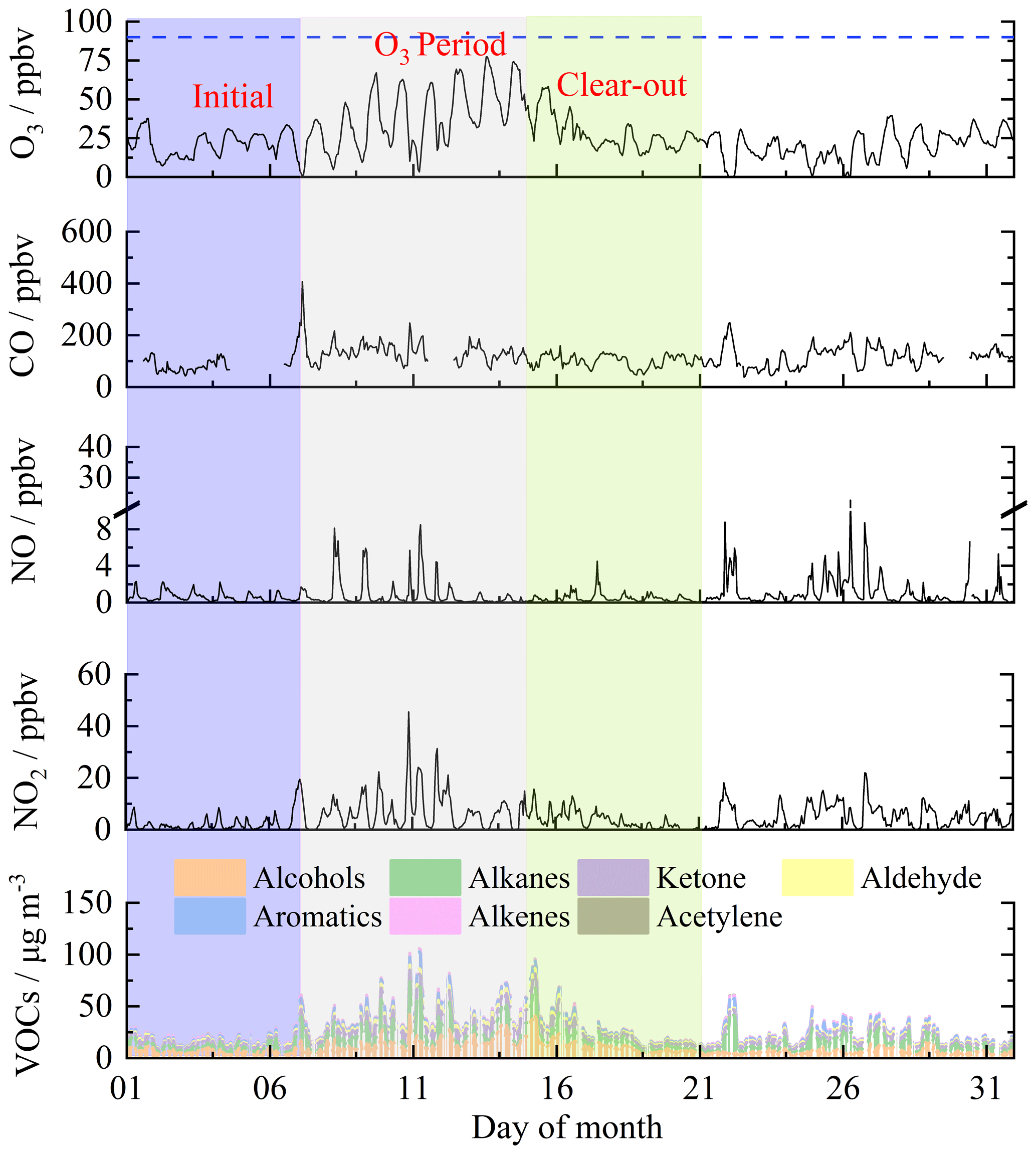
Figure 1 Time series of O₃, CO, NO, NO₂, and VOC groups at the Birmingham supersite. The dashed blue line denotes the national standard (90 ppbv) for hourly O₃ concentrations.

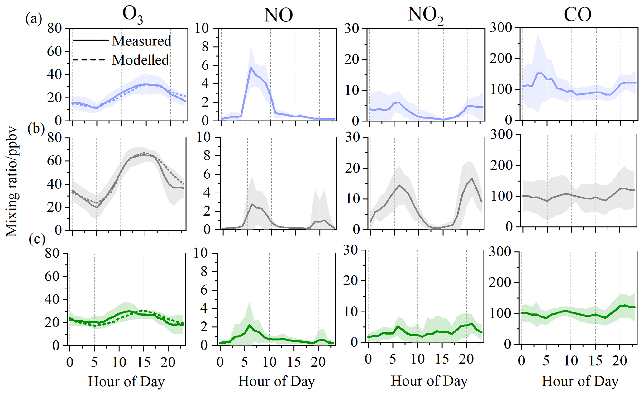
Figure 2 Diurnal variations in O₃, NO, NO₂, and CO during the (a) initial, (b) O₃, and (c) clear-out period. The shaded areas represent standard variations.

The general diel profiles for all selected VOCs, except for ethane, showed a bimodal pattern (Fig. S2). Concentrations were much higher during the night and lower during the day due to them being subject to photochemical losses during the daytime. The bimodal pattern is less apparent for methanol and acetone as they are abundant species originating from many anthropogenic sources in urban areas. For example, methanol was the most abundant species measured at a roadside in the UK using thermal desorption–gas chromatography coupled with flame ionization detection (TD-GC-FID) (Cliff et al., 2023). A separate study on gasoline and diesel vehicle exhausts reported that methanol and acetone were the largest OVOCs emitted (Wang et al., 2022). Gkatzelis et al. (2021) conducted a positive matrix factorization (PMF) analysis based on an observed VOC data set in New York City and concluded that acetone was the second most abundant species in the measurements and was mostly attributed to volatile consumer product emissions (90 %). (See Sect. 3.3 for further discussions on anthropogenic sources of OVOCs.)

3.2 Observation-based O₃ formation sensitivity

The in situ O₃ formation sensitivity was examined via the reaction rates of ozone precursors and an OH radical (OH reactivities; k(OH)) and RIR scales of ozone precursors, along with the chemical budgets of O₃ formation and loss. In initial and clear-out periods, k(OH) exhibited consistent diurnal patterns, ranging from 2.4 to 5.9 s⁻¹ (Fig. S3). In the O₃ period, k(OH) reached 9.0 and 8.7 s⁻¹ at approximately 07:00 and 20:00 UTC+1, respectively. A rapid increase in k(OH) was observed in the early morning (00:00–06:00 UTC+1). VOCs and model-generated species represented 60.5 %, 65.7 %, and 56.7 % of the total k(OH) in the three periods, respectively. NO_x and CO only contributed 10.2 %–27.9 % to the total k(OH). Among the VOC groups, alcohols exhibited the largest k(OH) in all periods, accounting for 5.0 %–6.9 % of the total k(OH). The diurnal production and loss of O₃ are shown in Fig. S4. The oxidation and photolysis of VOCs promoted the production of RO₂, and NO+RO₂ contributed 47.7 % of the O₃ production pathways in the O₃ period and 36.2 % and 39.8 % in the initial and clear-out periods, respectively. Considering O₃ destruction, OH + NO₂ was the most important pathway during morning (08:00–12:00 UTC+1), accounting for 73.5 %, 55.4 %, and 59.4 % of the O₃ destruction pathways in the three periods. The dominant OH + NO₂ contribution to O₃ destruction suggested that the in situ O₃ productions in all three periods were sensitive to VOC emissions to some extent.

In order to understand contributions to O₃ formation from direct emissions and secondary formations of OVOCs, we developed two modeling scenarios where (1) all OVOC species were constrained to the observed mixing ratio and (2) all OVOC species were unconstrained. Scenario 2 allowed for secondary formations of OVOCs by oxidations of their precursor VOCs. As shown in Fig. S5, secondary formations of OVOCs had little impact on O₃ formation in all periods. The simulation of O₃ production using the box model without constraining observed OVOCs slightly underestimated the average daily maximum O₃ mixing ratio and P(O₃) compared to the scenario with all observed OVOC species constrained. The underestimation for the average daily maximum mixing ratio of O₃ was 4.8 %, 6.9 %, and 5.1 % in initial period, O₃ period, and clear-out period, respectively. In this case, the underestimation of the average daily maximum P(O₃) was 5.1 %, 6.0 %, and 9.3 % in the three periods, respectively. The results demonstrated that in the Birmingham case study, primary emissions of OVOCs played a central role in the in situ ozone production.

The relative incremental reactivity of NO_x, CO, and anthropogenic VOCs (AVOCs, i.e., all measured VOCs except for isoprene) is shown in Fig. 3. The in situ O₃ production was most sensitive to anthropogenic VOCs with the highest positive RIR values (0.44–0.49). This is as anticipated, given earlier analyses demonstrating their role in determining k(OH) and O₃ production. The low RIR (0.03–0.07) for CO in all three periods indicated a minor contribution of CO oxidation to O₃ production. The high RIR (0.24) for NO_x was only observed in the O₃ period. Acetaldehyde showed the highest positive RIR (0.17–0.19) among the AVOCs, suggesting that the photolysis and oxidation of acetaldehyde were a limiting factor for O₃ formation. The important role of carbonyl compounds in atmospheric photochemistry has also been reported in previous studies, contributing up to 59.3 % of the O₃ formation in ambient environments in China, the United States, and Brazil (Qin et al., 2021; Q. Liu et al., 2022; Edwards et al., 2014). Alkanes and alcohols exhibited lower RIR values (0.02–0.04) despite their high mass concentrations.

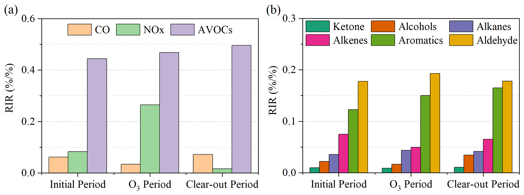
Figure 3 Modeled RIRs for (a) major O₃ precursors and (b) the AVOC groups during the photochemically active daytime (08:00–16:00 UTC+1) in the selected periods. (AVOCs stands for anthropogenic VOCs, i.e., all measured VOCs except for isoprene.)

3.3 Emission-inventory-informed O₃ production sensitivity tests

The trends in anthropogenic VOC emissions from 1990–2019 estimated by the NAEI are shown in Fig. S6. Over that period, the annual national emissions decreased by ∼ 69.0 %, from 2941 kt in 1990 to 911 kt in 2019. The reduction is partly attributed to more stringent controls for gasoline vehicle emissions, both tailpipe and evaporative/fugitive. In 2019, VOC emissions from on-road transport and fuel fugitive losses accounted for only 3.3 % and 13.7 % of the total mass of VOC emissions compared to 29.1 % and 26.9 % in 1990. Efforts have also been directed towards controlling industrial processes, commercial solvent usage, and combustion emissions, resulting in reductions of 66.8 %, 48.9 %, and 20.7 %, respectively, over that period. However, contributions from solvent usage to total VOC emissions over 1990–2019 showed only modest reductions in the 1990s and 2000s and, indeed, small increases in the most recent years (Fig. 4b). This slight growth in solvent usage is due to increasing emissions from solvent use in consumer products such as decorative products, aerosols, personal-care products, and detergents (NAEI, 2021). Solvent usage has become the largest contributory sector (33.7 %) to VOC emissions by 2019, followed by industrial processes (16.0 %).

As shown in Fig. 4a, the VOC speciation over the 1990–2019 period was dominated in mass terms by contributions from alkanes and alcohols, the former decreasing as gasoline sources declined and the other increasing as non-industrial solvent and food and drink industry processes' emissions followed a different pattern. Alkane emissions fell from 46.6 % to 30.6 % over that period. Further reductions in alkane emissions are expected from policies that aim to phase-out sales of new internal combustion engine vehicles in the UK (and in many other places) by 2035. The growth in the relative contributions of alcohols was primarily driven by increases in emissions of methanol and ethanol and, to a lesser extent, in 1-butanol and 2-propanol (Fig. 4c).

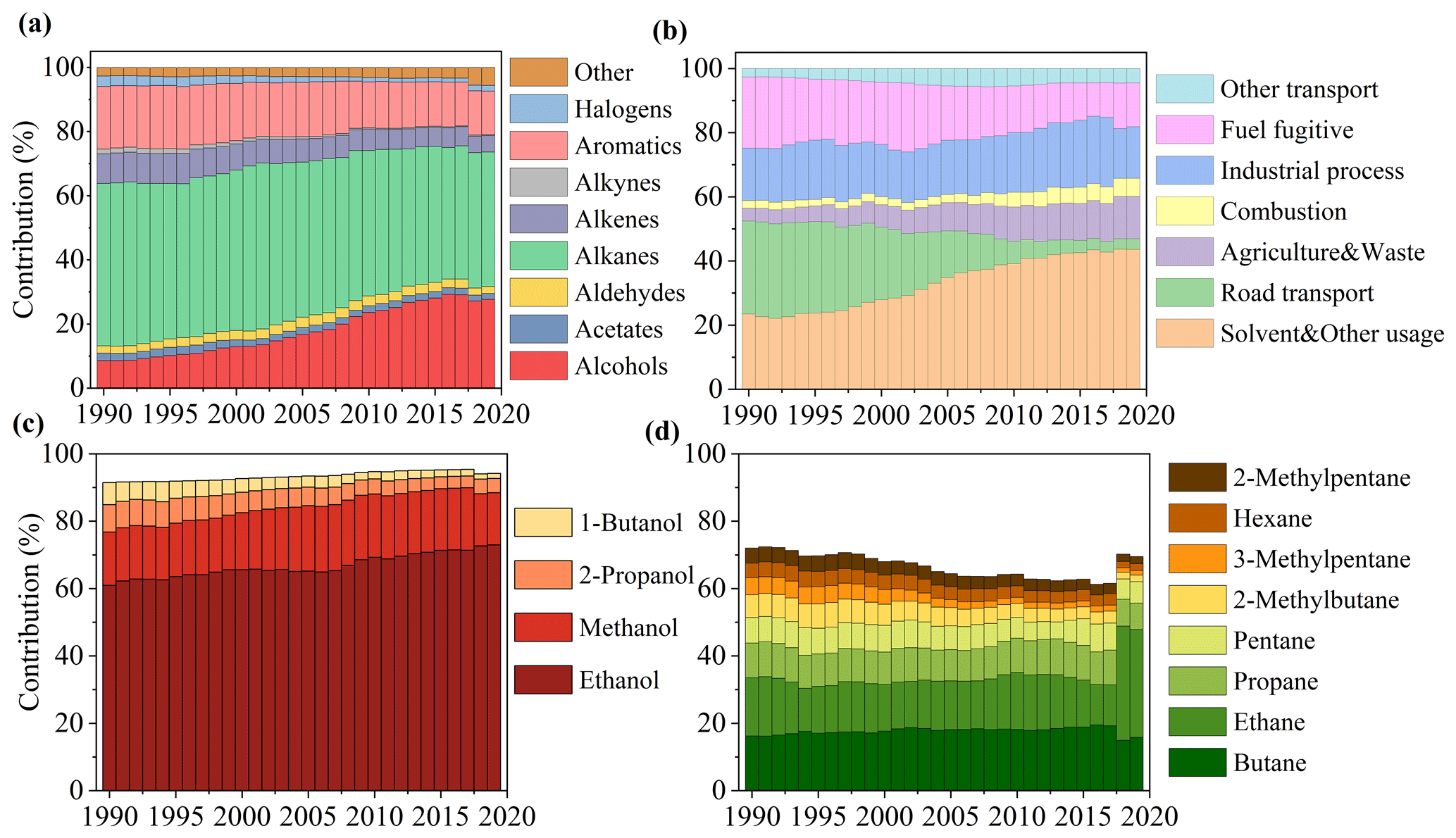
Figure 4 Contributions to annual national UK emissions of VOCs between 1990 and 2019 (a) by functional group, (b) by major emission-reporting sector, (c) for four individual alcohols in the overall sub-class of alcohols, and (d) for eight individual alkanes in the sub-class of all alkanes.

Figure S7 shows UK emission trends of individual species from different VOC classes. These highlight a national trend, present since 1990, of decreasing emissions of ethane associated with natural gas leakage; reductions in toluene and propane associated with on-road gasoline evaporation; and reductions in benzene, ethene, and acetylene associated with tailpipe exhaust. Meanwhile, the reduced emissions have been accompanied with increases in emissions of methanol and ethanol. The increase in methanol is largely attributed to increased emissions from car-care products (i.e., non-aerosol products) (Monks et al., 2020). The increase in ethanol is due to increased domestic and industrial solvent usage.

The NO_x, CO, and VOC speciation within the NAEI for each of the six major emission sectors was used to assign proportional sectoral contributions to the VOCs observed in Birmingham and hence to ozone production in the case study (Table S5). Isoprene was excluded from the analysis as it is assumed to have an entirely biogenic source. The six sectors are road transport (both of on-road exhaust emission and evaporative losses of fuel vapor), industrial processes, combustion, solvent usage, and fuel fugitive and agriculture emissions. This forms a key assumption that the VOCs at the observation site are affected directly and in the same proportion as VOCs reported in national amounts in the NAEI. We make this assumption since it provides a reasonable starting point for understanding how each VOC sector may influence O₃ production during a case study event; however, ozone formation might be sensitive to differing regional distribution in speciation. The attribution of VOC sources based on the NAEI data can be thought of as representative of this case study as a typical urban environment, but it might not hold for cities near large industrial VOC sources (i.e., oil refinery and industrial production sites) since they can significantly affect the composition and chemical reactivity of ambient VOCs.

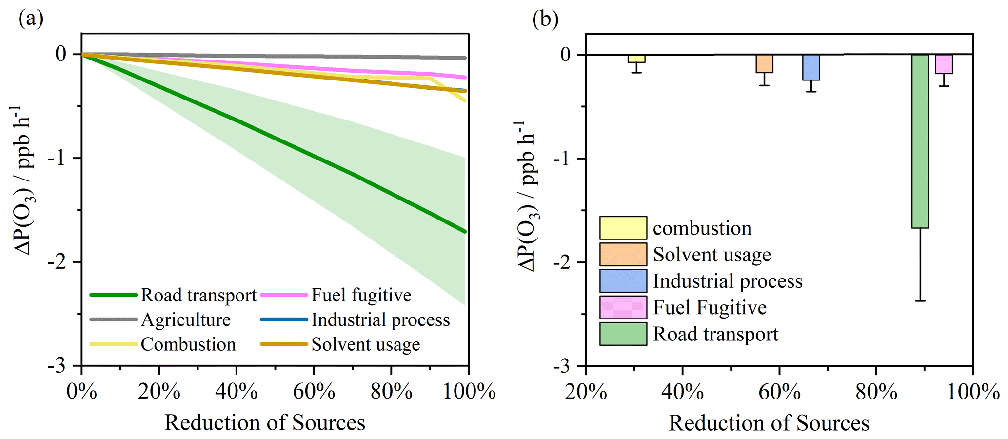
Figure 5 (a) Changes in P(O₃) in response to different reductions in VOCs, NO_x, and CO from different sectors for the Birmingham case study condition. (b) Changes in P(O₃) based on the NAEI estimated reductions in VOCs from different sectors between 1990 and 2019. The standard deviations represent variability in ΔP(O₃) during 08:00–16:00 UTC+1 in the O₃ period.

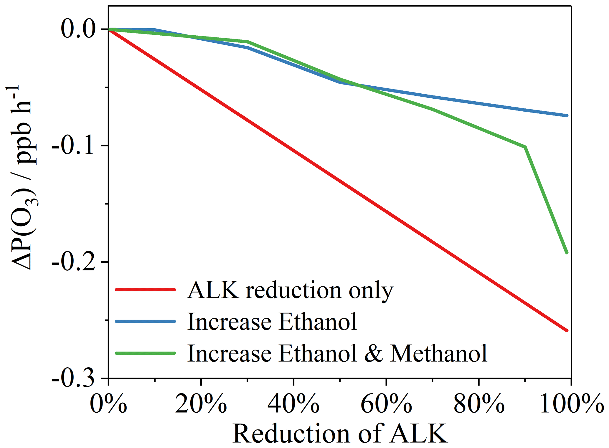
Figure 6 Reductions in ΔP(O₃) based on reducing alkanes (ALK) in the model (under case study conditions; red line), reducing alkanes but balancing the overall VOC amount with increased ethanol (blue line), and reducing alkanes but balancing the overall VOC amount with increased ethanol and methanol (green line).

Figure S8 shows the modeled RIRs for these sources in the initial, O₃, and clear-out periods. All the sources generally showed higher RIR values in the O₃ period. Road transport exhibited the highest positive RIR values in all periods (0.30–0.36), followed by industrial processes (0.06–0.09) and solvent usage (0.05–0.07). Despite being a relatively minor contributor to the mass of national VOC emissions (only 3.3 % of the total in 2019), road transport VOCs still played the most important role in local ozone photochemical chemistry in this case study.

Figure 5a shows the changes in P(O₃) during the O₃ period from 08:00–16:00 UTC+1, which might arise as a result of reductions in the individual sectors described above. For this analysis, emission changes in these sectors can be obtained by reducing model-constrained concentrations of VOCs, NO_x, and CO according to their contributions arising from individual emission sectors. This is a thought experiment, where under 2019 general observed atmospheric conditions (for, e.g., NO_x and CO), each of the VOC source sectors is then further reduced in isolation (from 2019 levels) and the effects on ΔP(O₃) are evaluated. Based on these scenarios, reducing emissions from the individual sectors all resulted in decreased P(O₃), as would be anticipated. Reducing ozone precursors arising from road transport would lead to a decreased P(O₃) of ∼ 1.71 ppbv h⁻¹ if that sector could be 100 % abated in the case study. This is expected because road transport is a source of photochemically reactive VOCs, including aromatics, aldehyde, and short-chain alkanes/alkenes. Other sectors showed more modest effects, with reductions in solvent-related VOCs being the next most significant lever to control ozone. Fully abating emissions of all industrial and solvent process emissions only resulted in a decreased P(O₃) of ∼ 0.35 ppbv h⁻¹ largely because they are dominated by ethanol and methanol with relatively low RIR values. Considering the real-world changes in VOC emissions over the period of 1990–2019, the very major reductions in road transport emissions have led to the largest effects on reducing P(O₃) (Fig. 5b). Whilst there have also been some very large reductions (94.6 %) in fuel fugitive emissions, the impact on P(O₃) reduction is modeled to have been relatively modest, being similar to industrial processes and solvent usage. It is important to acknowledge the limitation of this analysis. In the real world, reductions in ambient VOCs from the NAEI sectors are affected by photochemical loss rate and advection processes, potentially altering the proportion of VOCs that would be observed with each sector reduction at the measurement site. This would potentially be an important consideration if instantaneously radical budgets were being evaluated, but it is a less significant issue when integrating ozone production effects.

Further model runs were performed to better understand the impacts of the shift between alkanes and alcohol species on P(O₃), given trends showing decreasing alkane emissions and increasing alcohol emissions during the 1990–2019 period (Fig. 4). The modeled alkane concentrations in the case study were reduced by 10 %, 30 %, 50 %, 70 %, 90 %, and 99 %. This represents a downward trajectory in alkane emissions that would be anticipated as gasoline vehicles are slowly retired. Two further scenarios were then developed to sit alongside these reductions in alkanes. Firstly, the concentration of ethanol was increased to keep the overall total VOC concentrations in the model under case study conditions unchanged. Second, the concentrations of both ethanol and methanol were scaled upwards to keep the total VOC concentration unchanged. As shown in Fig. 6, reductions in alkanes alone resulted in decreased P(O₃) to a maximum of ∼ 0.26 ppbv h⁻¹ if fully abated. If that alkane reduction was balanced with increased ethanol and methanol, then ΔP(O₃) is reduced by a maximum of 0.19 ppbv h⁻¹. If alkane reductions were balanced by increasing ethanol alone, then P(O₃) still decreases but only up to 0.07 ppbv h⁻¹.

4 Conclusions

In this study, a typical high-O₃ event in Birmingham, United Kingdom, was chosen as a case study to investigate the impacts of changes to VOC emissions and speciation on urban O₃ production. The in situ O₃ formation sensitivity was split into three periods: initial, high-O₃, and clear-out. Results from OH reactivity, O₃ budgets, and RIR index showed that O₃ formation in all three periods was impacted by both VOCs and NO_x but was more sensitive to anthropogenic VOCs. The oxidation of alcohols and photolysis of acetaldehyde substantially contributed to in situ O₃ formation, especially in the high-O₃ period. The roles of anthropogenic VOC sources in urban O₃ chemistry were examined by integrating the NAEI speciation over the period of 1990–2019 into photochemical box model scenarios. Despite road transport only contributing 3.3 % of national VOC emissions in 2019, it still played the most important VOC role in the case study ozone photochemistry, when inventory contributions were mapped onto observed VOCs. Sequentially, the observed VOCs were reduced by the fractional contributions and speciation in the NAEI for six sectors to evaluate what impact abating different VOC-emitting sectors would have on P(O₃). Abating road transport VOCs in isolation would lead to a decreased P(O₃) by up to 1.67 ppbv h⁻¹, but abating other sectors, such as solvent use and fugitive fuels, had noticeably smaller effects. Despite emissions of VOCs from road transport falling very dramatically between 1990 and 2019, it remains one of the most powerful means of further reducing ozone in this typical UK case study. The wider shift in speciation reported in the NAEI from alkanes to alcohols was also examined using scenarios where emission reductions for alkanes were counterbalanced with increases in alcohols, all simulated for Birmingham case study conditions (for, e.g., NO_x and CO). Further reducing alkanes from present-day conditions to zero has a clear beneficial effect on reducing P(O₃) by up to ∼ 0.26 ppb h⁻¹. However, this benefit would, to a degree, be offset should alcohol emissions (for example, from food and drink and/or solvent use) increase to counterbalance those alkane reductions. Whilst simple alcohols are inherently less potent ozone-forming VOCs compared to the mixture of VOCs from road transport, avoiding future growth in emissions remains important since they weaken the long-term benefits of road transport electrification and the phase-out of internal combustion engine vehicles.