the Creative Commons Attribution 4.0 License.
the Creative Commons Attribution 4.0 License.
 | 28 May 2024
Air–sea interactions in stable atmospheric conditions: lessons from the desert semi-enclosed Gulf of Eilat (Aqaba)
Shai Abir
Hamish A. McGowan
Yonatan Shaked
Hezi Gildor
Efrat Morin
Accurately quantifying air–sea heat and gas exchange is crucial for comprehending thermoregulation processes and modeling ocean dynamics; these models incorporate bulk formulae for air–sea exchange derived in unstable atmospheric conditions. Therefore, their applicability in stable atmospheric conditions, such as desert-enclosed basins in the Gulf of Eilat/Aqaba (coral refugium), Red Sea, and Persian Gulf, is unclear. We present 2-year eddy covariance results from the Gulf of Eilat, a natural laboratory for studying air–sea interactions in stable atmospheric conditions, which are directly related to ocean dynamics.
The measured mean evaporation, 3.22 m yr−1, approximately double that previously estimated by bulk formulae, exceeds the heat flux provided by radiation. Notably, in arid environments, the wind speed seasonal trend drives maximum evaporation in summer, with a minimum winter rate. The higher evaporation rate appears when elevated wind, particularly in the afternoon, coincides with an increase in vapor pressure difference. The inability of the bulk formulae approach to capture the seasonal (opposite from our measurements) and annual trend of evaporation is linked to errors in quantifying the atmospheric boundary layer stability parameter.
Most of the year, there is a net cooling effect of surface water (−79 W m−2), primarily through evaporation. The substantial heat deficit is compensated by the advection of heat via northbound currents from the Red Sea, which we indirectly quantify from energy balance considerations. Cold and dry synoptic-scale winds induce extreme heat loss through air–sea fluxes and are correlated with the destabilization of the water column during winter and initiation of vertical water-column mixing.
- Article
(10133 KB) - Full-text XML
-
Supplement
(1828 KB) - BibTeX
- EndNote


Research on air–sea exchange of heat, gas, and momentum through surface fluxes provides valuable insights into the physical and chemical processes of marine environments that sustain diverse ecosystems, such as coral reefs. Accurate quantification of surface heat exchange is crucial for understanding the thermoregulation of the shallow water environment and basin-scale thermohaline dynamics.
The principle of energy conservation provides a comprehensive framework for quantifying thermoregulation in a marine environment; it is captured by the following equation:
The net radiation (RN) is the aggregation of the four components of the radiation budget, which are the downwelling shortwave radiation (DSW) and upwelling shortwave radiation (USW), related through the albedo term of the water, and downwelling longwave radiation (DLW) and upwelling longwave radiation (ULW). Latent heat flux (LE) and sensible heat flux (SH) can be accurately measured, and G refers to the change in heat storage in the water column. Net horizontal advection of heat in the water due to currents and tides is represented by QA. Therefore, in areas where reverse estuarine circulation occurs and where fluvial discharge and rain contribution are negligible, air–water interaction is directly connected to the general circulation through QA.
In recent decades, the measurement of the energy exchange components in marine and lacustrine environments has undergone significant advancements, particularly using eddy covariance (EC) towers that offer direct and accurate measurements of the turbulent fluxes of LE and SH (Lensky et al., 2018; Mor et al., 2018; Hamdani et al., 2018; McGowan et al., 2019; Rey-Sánchez et al., 2017; Pérez et al., 2020; Tau et al., 2022). These fluxes are commonly estimated by bulk formulae methods due to the accessibility of the method.
The bulk formulae method is a widely adopted approach to estimating surface energy fluxes due to its reliance on easily obtainable variables, namely sea surface temperature, air temperature, and a 2D wind measurement at 10 m. The bulk formulae method calculates the evaporation flux by multiplying the wind speed, specific humidity difference, and vapor transfer coefficient (Kondo, 1975). This approach to estimating surface energy fluxes relies heavily on the parametrization of the vapor transfer coefficient, which involves several assumptions and empirical relations for calculating the Monin–Obukhov length and the friction velocity (Fairall et al., 1996). Both can vary significantly in coastal regions according to the parametrization method (Bardal et al., 2018). While projects such as TOGA COARE (Tropical Ocean – Global Atmosphere Coupled Ocean Atmosphere Response Experiment; Fairall et al., 1996) have aimed to reduce uncertainties in the vapor transfer coefficient, their findings are primarily applicable to the tropical open ocean, where an unstable marine atmospheric boundary layer (MABL) is persistent. However, in stable atmospheric boundary layer (ABL) conditions that are common in sea areas where flow originates from land, like the northern Red Sea (as well as the Persian Gulf and the main body of the Red Sea), and coastal upwelling areas, large uncertainties remain in momentum and scalar flux estimation (Edson et al., 2007). These shortcomings indicate that discrepancies between the EC method and bulk formulae may originate from the vapor transfer coefficient parametrization. Thus, to overcome these uncertainties, a comparison with direct measurements is needed. Apart from the effect on each air–sea flux, the uncertainties are propagated into the energy balance of the system, and, therefore, there is no energy closure, and the energy balance closure problem is unresolved (Yu, 2018).
In coastal regions, synoptic-scale variability alternates between regional mean flow and secondary circulation, impacting the intensity, duration, orientation, and travel distance of cross-land–sea winds (Allouche et al., 2023). Processes spanning from diurnal to seasonal cycles, involving local micrometeorological parameters and variability due to synoptic-scale forcing, play a crucial role in influencing the energy balance partitioning and thermoregulation of shallow marine environments. Synoptic-scale forcing, which induces changes in humidity, wind speed, and air temperature, can rapidly influence water temperature and the overall energy balance (Abir et al., 2022; Genin et al., 2020; MacKellar and McGowan, 2010; Papadopoulos et al., 2013). These findings underscore the importance of understanding how the energy balance of marine environments behaves on a diurnal to seasonal cycle in response to local and regional micrometeorological factors and irregular synoptic-scale events. Recognizing these mechanisms as a research priority is crucial as they are applicable to other regions experiencing strong land–sea winds (Azorin-Molina and Chen, 2009).
This paper presents a comprehensive analysis of continuous 2 years of EC measurements of heat and water vapor over the northern Gulf of Eilat (GoE). These data allow us to accurately characterize, for the first time, the diurnal and seasonal cycles of energy balance partitioning in an arid semi-enclosed sea. The GoE is not only a model for other arid semi-enclosed seas; it has been proposed as a natural refugium for corals, as corals within the gulf show a unique thermal resistance by being able to survive bleaching in extremely high temperatures (Fine et al., 2013; Abir et al., 2022). Thus, the gulf is a critically important ecological and economic zone for Israel, Egypt, Saudi Arabia, and Jordan and understanding the processes controlling its heat balance is of wide interest.
The results show discrepancies with previous studies' estimates by bulk formulae, both in mean rate and seasonal trend. Our analysis of the origin of the gap between the bulk formulae method and our direct measurements highlights the features that should be improved in the bulk formulae approach when applied in semi-enclosed seas. We also analyze synoptic-scale events as a methodological case study to demonstrate how synoptic-scale events affect the energy balance. By characterizing air–sea interaction processes we gain insight into the thermoregulation processes of semi-enclosed seas and thermohaline circulation processes.
The structure of the paper is as follows: in Sect. 2, we describe the study-region-specific setting and previous air–sea fluxes reports, the study methods, and the data. In Sect. 3, we present the results of the study in the context of diurnal to seasonal cycles, comparisons with bulk formula, and synoptic-scale case studies. In Sect. 4, we discuss the effect of the air–sea fluxes on thermoregulation processes, estimates of the advection flux, bulk formulae deviation from EC results, and synoptic-scale events as preconditioning to basin winter vertical mixing of the water column.
2.1 Study region
The study was conducted over the northwestern shore of the GoE, Israel (Fig. 1a and b), a narrow (< 25 km), deep (maximal depth of 1800 m) sea semi-enclosed by a hyper-arid desert. The GoE is connected to the Red Sea through the Straits of Tiran in the south. Local winds are channeled by the Arava Rift Valley, bringing (most of the time) a dry terrestrial northeasterly wind (along gulf component) to the northern GoE (Fig. 1e). During winter, less-common southerlies affect the region. These are channeled by the GoE basin, traveling a longer distance over the sea compared to the prevailing northerly winds (Afargan and Gildor, 2015).
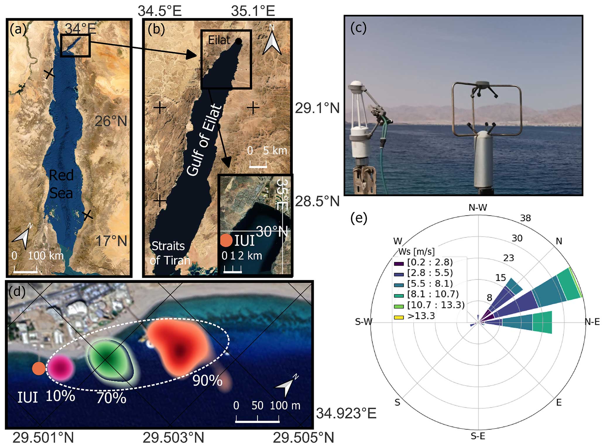
Figure 1Location map and site description. Satellite images of (a) the Red Sea and (b) the Gulf of Eilat (Aqaba). The insert in (b) shows the eddy covariance station location at the IUI. (c) The eddy covariance instruments, IRGA, and 3D wind anemometer. The footprint heatmap is presented in (d); pink (10 %), green (70 %), and red (90 %) represent the percentile of the distances from which the data were collected by the EC, and the dashed white line is a schematic representation of the footprint area. (e) Wind rose diagram for the entire observation period; values in the legend are wind speeds (in m s−1; September 2020–September 2022), and centric contours are percentiles from the observations. Image copyright: (a, b) data SIO, NOAA, US Navy, NGA, GEBCO image © Landsat/Copernicus, (d) © 2022 CNES/Airbus. The source for the image in the insert in (b) is data SIO, NOAA, US Navy, NGA, GEBCO, © 2022 TerraMetrics, © 2022 CNES/Airbus, © 2022 Maxar Technologies.
During summer (June, July, August – hereafter JJA), the prevailing atmospheric synoptic circulation is a low-pressure system centered northwest of Israel (Persian Trough). During winter, the common synoptic systems are the Cyprus Lows, Red Sea Trough (RST), and Siberian High. The Red Sea Trough (RST) is characterized by a region of surface low pressure, extending from the Red Sea to the coast of Turkey; it is common during transitional seasons and winter (Dayan et al., 2012). During winter (December, January, and February – hereafter DJF) anti-cyclonic synoptic flow (an intensified Arabian High, an extension of the Siberian High) associated with surface high-pressure systems can cause strong, cold, and dry westerly winds over the Red Sea. These anti-cyclonic flows result in extreme heat loss events through the latent and sensible heat fluxes (stronger than −400 W m−2) (Menezes et al., 2019). In contrast, low-pressure systems are associated with lower heat loss values (values from −100 to −50 W m−2) as these events are accompanied by warm and humid southerly winds (Papadopoulos et al., 2013). However, research on extreme heat loss events has been done on coarse satellite data (∼ 0.5°); therefore, an accurate representation of the GoE is lacking due to its small dimensions and indirect flux estimation (conducted using the OAFlux and MERRA-2 datasets).
Short periods of EC measurements conducted at the GoE (Rey-Sánchez et al., 2017; Abir et al., 2022) during summer, where cooler water underlies warmer dry air, demonstrate an oasis effect, which promotes evaporative cooling measured to be > 10.3 mm d−1, thus showing discrepancies between the evaporation rates estimated by bulk formulae during summer (∼ 3 mm d−1) and maximum evaporation during winter (11 mm d−1). These bulk formulae explained the higher winter evaporation by the ABL instability due to warmer surface water than the overlying air (the range of bulk formulae estimation being [1.6,3.65] m yr−1; Ben-Sasson et al., 2009; Eshel and Heavens, 2007; Sofianos et al., 2002; Assaf and Kessler, 1976). These findings highlighted the need for the implementation of accurate and direct measurement methods of the turbulent fluxes to better understand the complex energy balance dynamics in the GoE. Similar characteristics probably exist in other desert-enclosed basins, such as the Red Sea or the Arabian Gulf.
The general circulation model of the GoE, which was originally proposed by Klinker et al. (1976), was characterized as reverse estuarine circulation and was the widely accepted model. The model postulated that buoyancy circulation driven by heat loss and evaporation is the primary driving force behind the GoE circulation. Biton and Gildor (2011b) proposed a seasonally varying model, where the maximal exchange flux between the northern Red Sea and the GoE occurs during the re-stratification season (April to August). It is driven by density differences between the basins, while atmospheric fluxes counteract this exchange flow. They attributed the observed warming of the surface primarily to the advection of warm water from the northern Red Sea, with a smaller contribution from surface heating.
Since the winter of 2011–2012, the vertical winter basin overturning (vertical mixing) did not exceed a depth of ∼ 500 m until the winter of 2021–2022, which exceeded 700 m (Shaked and Genin, 2022). The depth of the mixing strongly affects the nutrient budget of the shallow water at the GoE by transporting deeper water enriched with nutrients to the surface.
The alongshore currents in the northwestern terminus shore, where the EC was located, typically flow from north to south in response to tides and winds (Berman et al., 2000, 2003). Daily shallow water temperature at the GoE varies from ∼ 21.5 °C (minimum 20.5 °C) during winter to ∼ 27.5 °C (maximum 30.5 °C) during summer (based on measurements from 2007 to 2021 conducted by Israel's National Monitoring Program, NMP). The average annual open-sea SST has increased by an average rate of more than 0.5 °C per decade since 2004 (Shaked and Genin, 2022).
2.2 Methods
2.2.1 Instruments
Eddy covariance tower
The eddy covariance system consisted of an open-path infrared gas analyzer (IRGA; model LI-7500; LI-COR, Inc., USA) coupled with a 3D ultrasonic anemometer (YOUNG 81000; R.M. Young), both recorded at 20 Hz using a CR1000X data logger (Campbell Scientific, USA). The instruments were positioned 45 cm apart on the same vertical level. The station (Fig. 1c) was mounted on a ∼ 7 m tall mast above the mean sea surface, ∼ 36 m offshore, positioned at the end of the wharf (29.510748° N, 34.917669° E) of the Interuniversity Institute for Marine Sciences (IUI). Solar and maritime radiation exchanges were measured by a CNR1/CNR4 net radiometer (Kipp & Zonen BV, the Netherlands) mounted on the south side of the wharf of the IUI station, extending ∼ 1.5 m out from the wharf and 1.5 m above the water surface. Air temperature and relative humidity were measured by HC2S3 probes (Campbell Scientific, USA). Water skin temperature was measured by an SI-4H1 infrared radiometer (Apogee Instruments, Inc.). Water temperature (measured at a water depth of ∼ 1 m) at IUI as well as relative humidity, air temperature, DSW, and wind measurements for gap-filling purposes were obtained through the NMP at the GoE (http://www.meteo-tech.co.il/eilat-yam/eilat_en.asp, last access: 25 May 2024). The LI-COR 7500 open-path gas analyzer and net radiometer were regularly washed to ensure the sensors were free of salt and dust.
High-frequency hydrographic data
We used an ocean mooring equipped with a Del Mar Oceanographic Wirewalker, hereinafter Wirewalker. The Wirewalker is purely mechanical and profiles continuously, with wave energy driving the buoyant profiler downward. Upon reaching the deepest user-specified sampling depth, it freely ascends along its suspension cable (a.k.a. profiling wire), nearly completely decoupled from mooring motion. The Wirewalker was equipped with an RBRconcerto CTD. The RBRconcerto CTD was programmed to work in directional mode, with a fast sampling rate (8 Hz) in the ascending direction and a slow sampling rate (1 Hz) while descending. In this work, we used only upcast data. The RBRconcerto CTD measured the temperature and salinity from 3 m down to 150 m between 10 November 2021 at 06:00:00 and 23 November 2021 at 12:14:55, 8 February 2022 at 06:22:35 and 3 March 2022 at 08:34:35, and 6 July 2022 at 08:00:00 and 27 July 2022 at 10:43:52 GMT+0.
2.2.2 Footprint and data quality
EC measurement footprints were calculated using the EddyPro program (LI-COR Biosciences, 2021) (Fig. 1d). EddyPro uses three footprint models (Kljun et al., 2004; Kormann and Meixner, 2001; and Hsieh et al., 2000; coded 0–2 in the dataset attached to this paper; Abir et al., 2023); however, in this research, the Kljun et al. (2004) model was almost exclusively utilized. To minimize data contamination of the footprint, a wind direction filter was applied to exclude wind from land (the excluded wind directions being 225–360°). The water surface is not static due to water motion (currents, waves, and tides); however, we can regard it as a static surface, since the water motion velocity is 2 orders of magnitude smaller than wind velocity. Maximum tidal changes in the GoE are small and may offset the 90 % footprint distance by only a few tens of meters – i.e., 622 to 700 m (∼ 10 % change) – and are therefore considered not to have a great effect on energy flux measurements. In addition, low-quality data were excluded and, using the Foken flag method, aggregated by EddyPro in three categories (Foken et al., 2004, https://www.licor.com/env/support/EddyPro/topics/flux-quality-flags.html, last access: 25 May 2024) (data categorized as Foken flag = 2 were excluded); a post-processing manual spike removal was conducted so that latent heat (LE) and sensible heat (SH) fluxes were restricted between −50 and 1100 W m−2 and ± 250 W m−2, respectively. The resulting percentage recovery of 30 min mean flux data was 45 %46 % () before gap filling, which is typical of the recovery rate of shoreline-mounted EC stations (Gutiérrez-Loza and Ocampo-Torres, 2016). During April–June 2022, the EC station recorded at a frequency of 4 Hz due to an error; the reader is referred to Fig. S3 in the Supplement for an analysis of the uncertainty in the fluxes due to this error, in which the mean difference for the latent and sensible heat is 30 and 3 W m−2 (respectively), between 4 and 20 Hz measurements.
2.2.3 Post-processing
This subsection describes the calculation of additional meteorological parameters relevant to the energy balance analysis and the assumptions and methodologies of the calculation of the energy balance equations (Eq. 1).
Half-hourly energy fluxes (Abir et al., 2023) were obtained using the EddyPro program (LI-COR Biosciences, 2021). The program was run in express mode, which includes defaulted filters and corrections – wind component double rotation, block averaging, and spectral corrections for the separation of the wind anemometer and the IRGA (EddyPro 7 Software, 2023).
The contribution of rain to the energy balance is negligible as the study site is located in a hyper-arid desert (annual average precipitation between 1990 and 2020 is 23 mm; Meteorological Service, 2023). The heat exchange across the seabed is also considered to be negligible in this study due to its typical values usually being minor contributors to the energy balance equation (Pivato et al., 2018; Shalev et al., 2013). QA is hard to measure in the GoE since geopolitical constraints prevent across-gulf measurements of currents and temperatures, and in this paper, it is inferred as a residual from the surface energy fluxes (RN, LE, and SH) and the change in heat storage. When the change in heat storage measurement is not available, then the seawater residual is reported (QSWR), which is the net surface exchange () (McGowan et al., 2010).
Change in heat storage in the water column (G) was obtained by first calculating the heat storage as followed from the Wirewalker CTD measurements:
where Hg is the total heat of the profile water column in J m−2, ρ is the seawater density, Cp is the heat capacity at a constant pressure of seawater ( []), and ΔZ (in m) is the 1 m water layer thickness. Then, the heat storage was differentiated in time for the change in heat storage:
where G is the change in heat storage in W m−2, ΔHg is the change in total heat, and the Δt is in seconds (for the full description of the calculation the reader is referred to Sect. S2 in the Supplement).
The vapor pressure difference between the water surface and the overlying air is given by
where Tw and Ta are the water and air temperature, respectively, and are given in degrees Celsius; esat(T) (in mbar) is the saturation vapor pressure by the Magnus–Tetens formula; β is water activity set to be 0.98, which is a typical value for seawater (Sverdrup et al., 1942); RH is the relative humidity; ew and ea are the water and air vapor pressure (in mbar), respectively; and Δe is the vapor pressure difference (in mbar).
2.2.4 Gap filling
Gaps (gap duration of ∼ 6 h) exist in the relative humidity (RH), wind speed (Ws), water temperature (Tw), and air temperature (Ta), where data were missing due to station quarterly maintenance. These gaps were filled first by replacing the missing data with the data from an adjacent sensor from the NMP. Following that, a bi-linear, periodic, trended interpolation (Morin et al., 2014) was used for small gaps.
Due to the malfunction of the downward-facing pyrgeometers of the CNR1 (September 2020–April 2022), the ULW was calculated in W m−2 from the water temperature measurement according to the Stefan–Boltzmann law:
where ε is the emissivity (ε=0.985), σ is the Stefan–Boltzmann constant ( ), and Tw is the water temperature in kelvins.
The DLW was calculated based on Bignami et al. (1995); cloud coverage effect on the calculation was determined to be negligible (Ben-Sasson et al., 2009):
Equations (5) and (6) were used to gap-fill during the period where the station measured in 4 Hz mode, which interfered with the data collection of the CNR4 and general gap filling.
The USW was calculated as a fraction of the downwelling shortwave radiation (Paynes, 1972):
The DSW was gap-filled by taking the measurement from the adjacent NMP sensor, and Eq. (7) was used to fill gaps in the USW. The difference between the calculated net radiation mean and the measured net radiation mean was 50 W m−2, which is 20 % of the measured mean (during a month where there were no gaps in the net radiometer data).
To fill gaps in LE and SH, an artificial neural network (ANN) algorithm was utilized (Mahabbati et al., 2021). The algorithm was implemented with the Python sklearn.neural_network.MLPRegressor package when the hyperparameters (learning rate, hidden layer, and maximum iteration number are specified in the Figs. S1 and S2) were chosen by a grid search cross-validation algorithm (for the evaluation of the ANN performance refer to Figs. S1 and S2). Following the gap-filling procedure, the resulting percentage recovery of 30 min mean flux data was > 99 %.
2.2.5 Bulk formula
The bulk formula used to compare air–sea fluxes at the GoE is the COARE 3.6 algorithm (Fairall et al., 1996). We used the NMP measurements as input data for the algorithm; hence, this analysis is comparable to previous works that utilized these data and for future reference. The bulk Richardson number (RiB), which is used by the bulk formula to indirectly parametrize the stability parameter (ζ) (for more details see Sect. S3), is given by
where g (m s−2) is the gravity acceleration, Θ and Θ0 (K) are the potential temperatures calculated from Ta and Tw, respectively; z (m) is the measurement height of the wind speed; Ws is the wind speed (m s−1); and f(TaΔq) is a correction term for the potential temperature difference due to the air lapse rate and cool skin effect (Δq is the specific humidity difference between the water surface and the air in g kg−1). The modeled friction velocity and ABL stability are compared to the directly calculated friction velocity and ABL stability from the EC 3D wind anemometer. To compare the bulk formula vapor transfer coefficient (Ce) to the EC measurements, we calculate Ce from the EC LE flux:
where ρa (kg m−3) is the air density and Lv (J g−1) is the latent heat of vaporization of water, both calculated following Fairall et al. (1996).
3.1 Micrometeorology and water temperature
The 2-year (September 2020–September 2022) measured local micrometeorology and the mean diurnal cycles per season are presented in Figs. 2 and 3, respectively. The mean air temperature and relative humidity during the observation period were 25.9 °C and 42 % (respectively).
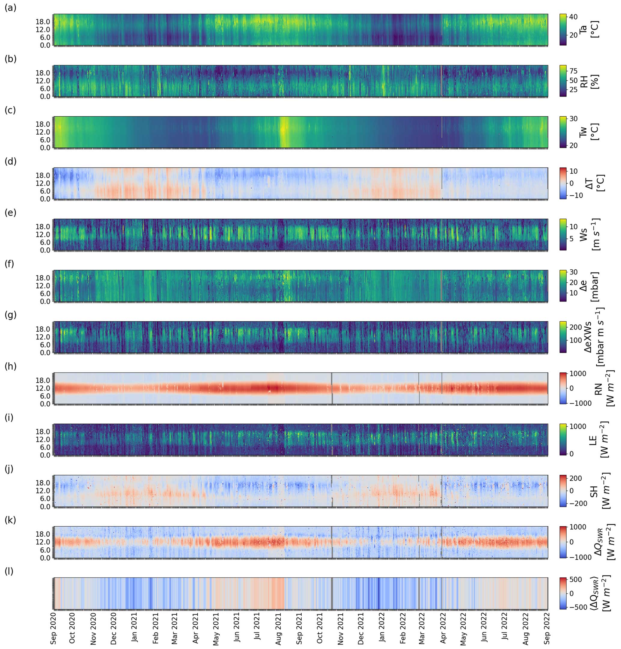
Figure 2Diurnal (LT) and seasonal variations (y and x axes, respectively) of the following parameters, measured during September 2020–September 2022: (a) air temperature (Ta), (b) relative humidity (RH), (c) water temperature (Tw), (d) water–air temperature difference (ΔT), (e) wind speed (Ws), (f) vapor pressure difference (Δe), (g) Δe×Ws, (h) net radiation (RN), (i) latent heat flux (LE), (j) sensible heat flux (SH), (k) seawater residual (QSWR), and (l) daily seawater residual change (〈ΔQSWR〉).
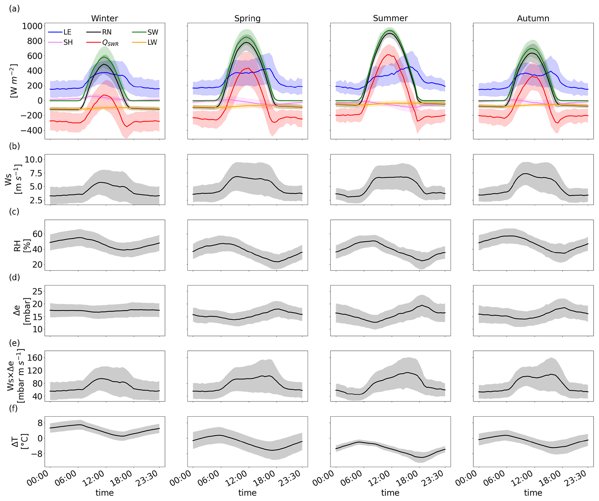
Figure 3Seasonal mean diurnal (LT) cycle of micrometeorological and flux variables (winter: December–January–February, DJF; spring: March–April–May, MAM; summer: June–July–August, JJA; autumn: September–October–November, SON) and in the shaded area the ± 1 SD span. (a) Energy fluxes, (b) wind speed (Ws), (c) relative humidity (RH), (d) vapor pressure difference (Δe), (e) vapor pressure difference product with wind speed (Ws×Δe), and (f) water–air temperature difference (ΔT).
The air temperature varied between the winter seasonal mean value of 18.7 °C and the summer seasonal mean value of 32.1 °C. Relative humidity seasonal mean varied between a value of 47 % during autumn (September, October, November – hereafter SON) and winter (DJF) and a value of 39 % during summer (JJA) and spring (March, April, May – hereafter MAM) (Appendix A). The water temperature mean value was measured to be 24.7 °C; Tw was characterized by a low mean water temperature value of ∼ 23 °C during winter and spring, which then shifts to summer and autumn, with higher mean values of ∼ 26 °C. Consequently, the water at the GoE is warmer than the overlying air from November to March (Figs. 3f and S4). The northeasterly (mean direction of 23°) dominating winds have a mean seasonal wind speed of ∼ 4.9 m s−1, observed through spring, summer, and autumn. The wind speed reaches the minimum value of 4.1 m s−1 during the winter (minimum out of the mean values per season). The seasonal mean diurnal cycle of wind speed (Figs. 3b and S4) can be differentiated into two common cycles: double peak and the bell-shaped curve. Both types start to increase from the lower nighttime values at ∼ 06:00 LT, reaching the first daily maximum of > 6 m s−1 at ∼ 10:30 LT; eventually, at ∼ 15:00 LT, the wind speed decreases to < 5 m s−1 in winter and at 17:00–17:30 LT during the rest of the year. The diurnal variations in Δe (Eq. 4; Fig. 3d) were characterized by daily mean minimum values occurring at ∼ 09:00 LT (14 mbar) and the daily mean maximum values at ∼ 18:30 LT (18 mbar). Additionally, from April–October, the mean daily variations in Δe are significantly more pronounced, concurrently with the water–air temperature difference (ΔT) and the RH daily variations. In winter, the highest value of seasonal mean Δe is obtained (17.3 mbar) due to the positive ΔT (Fig. 3f); however, during summer, higher mean maximum daily values (26.3 mbar) are obtained due to the strong diurnal variations.
3.2 Surface heat flux
The 2-year (September 2020–September 2022) measured surface fluxes and their mean diurnal cycles per season are presented in Figs. 2 and 3, respectively.
3.2.1 Net radiation
The observation period mean RN value was 157 W m−2, where positive values represent flux of energy from the atmosphere into the water surface. The net radiation mean diurnal cycle was of the characteristic bell shape, and seasonal mean values varied between 55 W m−2 in winter and 252 W m−2 during summer (Fig. 3a). Nighttime net radiation values were negative, with stronger ULW than DSW (Fig. 3a) and with positive RN values during the daytime. The daily mean maximum temperature of Tw lags behind the mean daily maximum RN by 2.5 h, while the daily mean maximum Ta lags by 5.5 h.
3.2.2 Latent heat
The mean LE flux during the observation period was 255 W m−2 (3.22 m yr−1 of evaporation). Latent heat flux seasonal mean varied between the minimum values during winter (232 W m−2) and the maximum during summer (276 W m−2). As described in Sect. 3.1, for the Ws mean diurnal cycle, the LE flux mean diurnal cycle is categorized into two cycles, double peak and bell-shaped curve, where from mid-spring (April/May) to mid-autumn (September/October) there was a clear double peak in the diurnal LE cycle. The first peak coincides with the daily maximum wind speed (∼ 10:00 LT), whereas the second peak, which was the absolute daily maximum (mean max value of 462 W m−2), coincides with the product of the Ws and the Δe (Fig. 3e) at 15:30 LT. The product of the Ws and the Δe, as prescribed by the bulk formulae approach, has the highest correlation with the LE flux (0.99; Fig. 4b). However, at the GoE, the high correlation originated mostly from the correlation with the wind speed profile of 0.97 (Fig. 4b). The high correlation was visible in the temporal variations in both diurnal and seasonal plots (Figs. 3 and 4).
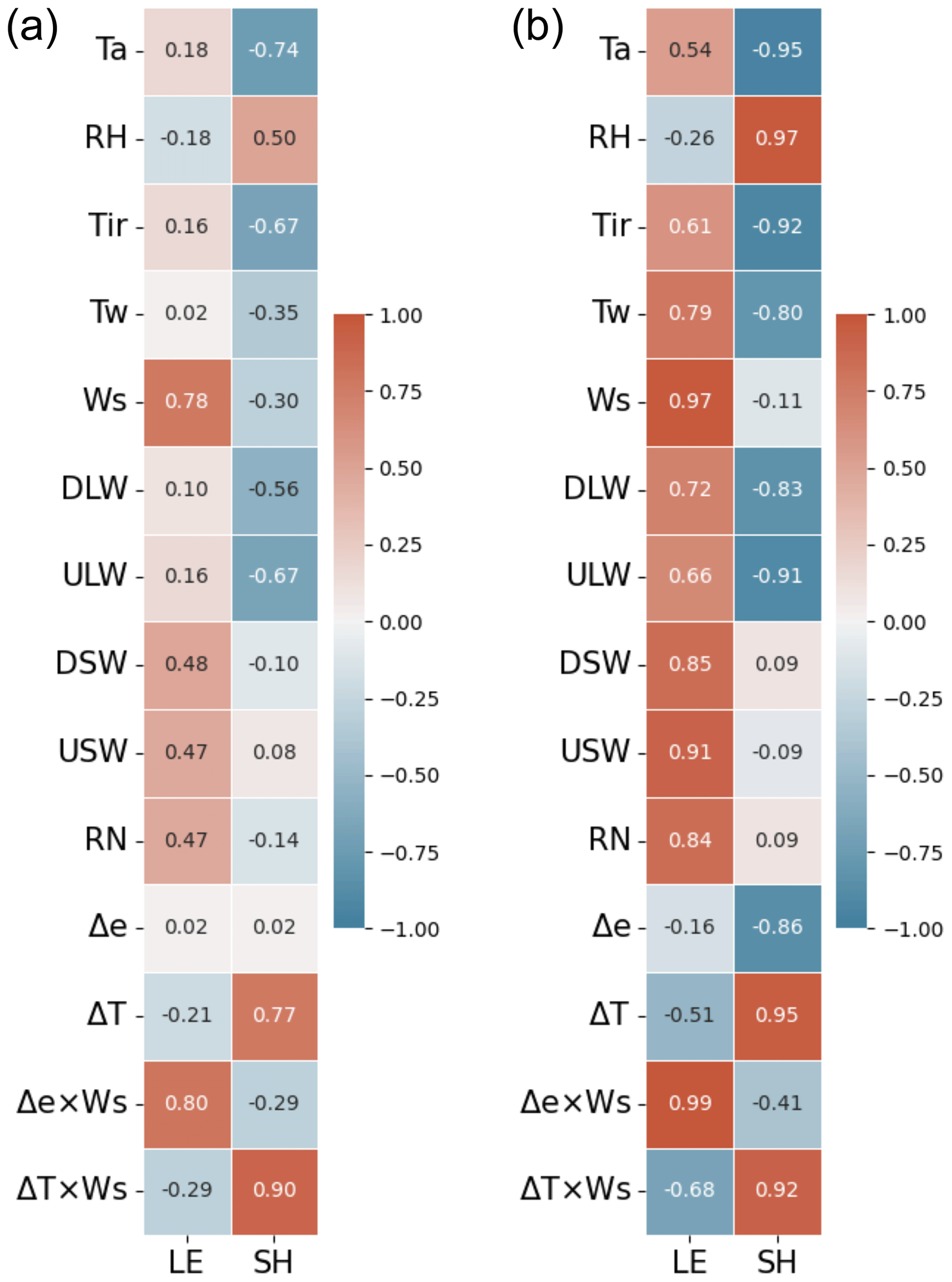
Figure 4Pearson's correlation matrix for (a) 30 min data and (b) daily mean data of the sensible and latent heat fluxes with micrometeorological and radiation flux variables.
3.2.3 Sensible heat
The SH flux mean value throughout the observation period was −20 W m−2. Concurrent with the seasonal air–sea temperature difference cycle, the SH flux, on average, transfers heat from the water to the atmosphere during winter (winter mean values of ∼ 19 W m−2) and continues outside of winter until September and May (Figs. 3a and S4). The spring-to-autumn mean seasonal value of SH flux of ∼ (−32) W m−2 corresponds to the relatively cool sea surface in a hot desert surrounding. Similarly to the LE flux, the SH flux is highly correlated with the product of Ws and a gradient air–sea temperature difference (Pearson r=0.92; Fig. 4b).
3.2.4 Evaporation estimations – direct EC measurements vs. bulk formula
Figure 5 presents the bulk formula calculation with the COARE 3.6 algorithm of ABL meteorology parameters and the latent and sensible heat fluxes throughout the 2-year observation period compared to the EC-obtained variables.
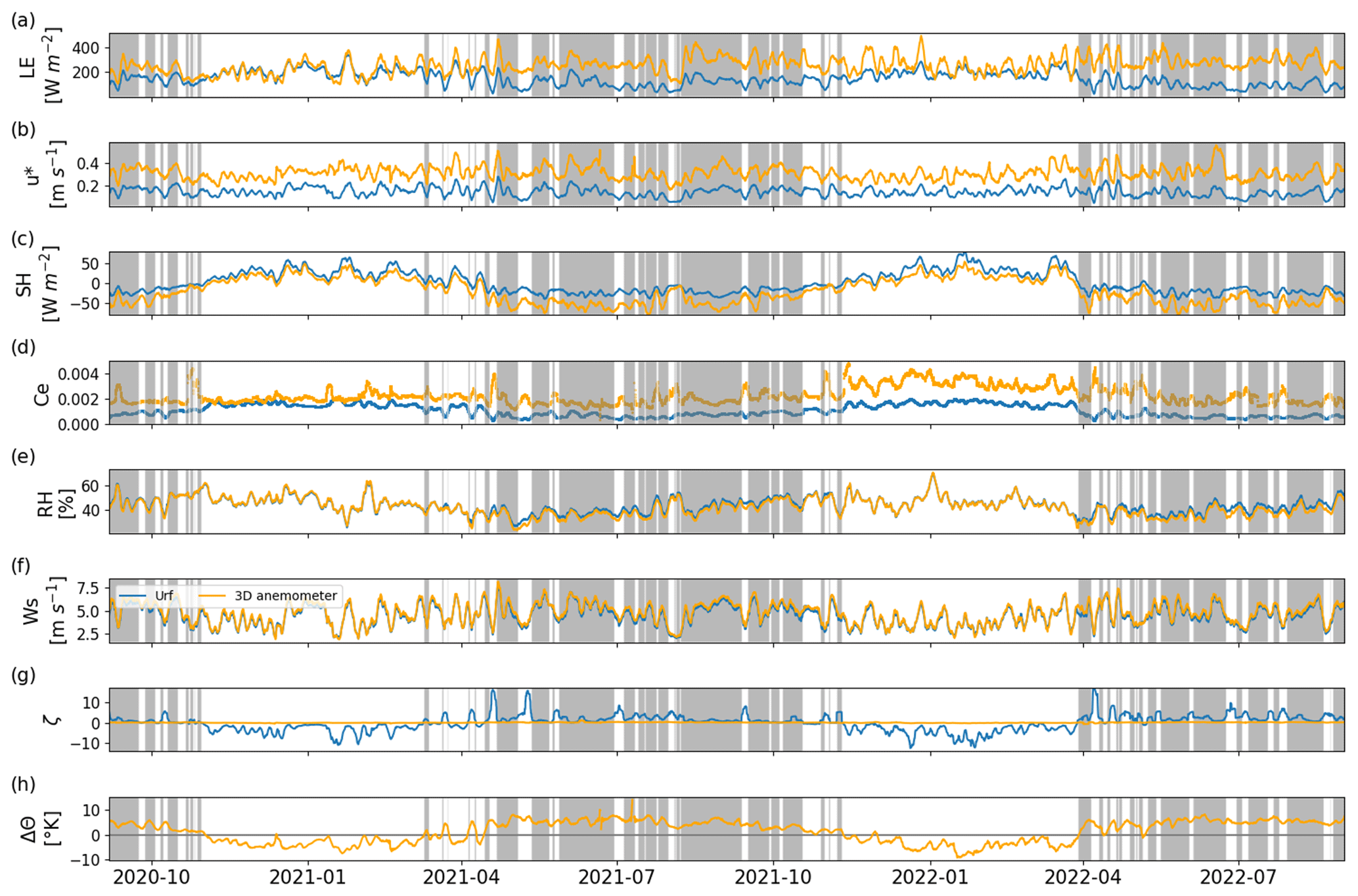
Figure 5Comparison between the 3 d (LT) rolling average EC-measured sensible and latent heat fluxes and meteorological parameters (orange) and the bulk formula calculation using the TOGA COARE 3.6 algorithm (blue), computed with the NMP micrometeorological data. Shaded in gray are instances where the TOGA COARE 3.6 algorithm bulk Richardson number is within the range of 0–0.2, indicating stable conditions. The wind speed panel compares the measurements of the 3D sonic anemometer and the interpolated referenced height (7 m) of the TOGA COARE 3.6 algorithm. The panels show (a) latent heat (LE), (b) friction velocity (u∗), (c) sensible heat (SH), (d) vapor transfer coefficient (reverse calculated from the EC measurements Eq. 9), (e) relative humidity (RH), (f) wind speed (Ws), (g) stability (ζ), and (h) air and water potential temperature difference (Δθ). Key variations between the EC method and the bulk formula are higher evaporation rates measured with the EC system during stable conditions, consistent higher friction velocity measured with the 3D sonic anemometer, and low variation within the stability parameter calculated with the EC system.
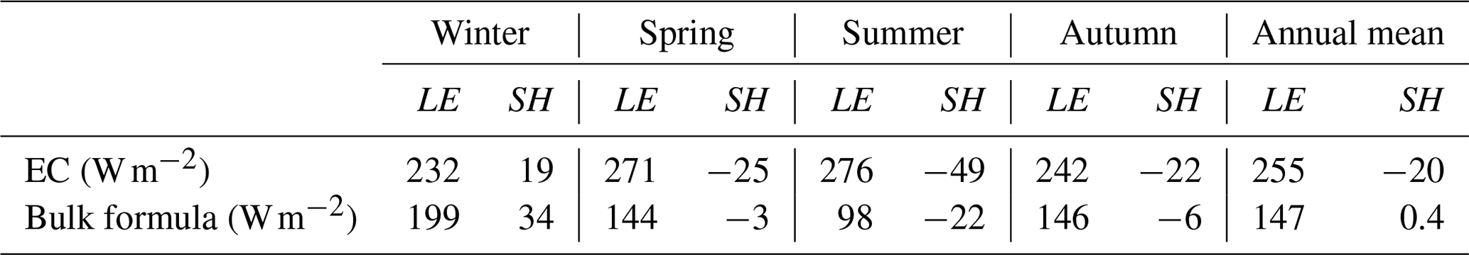
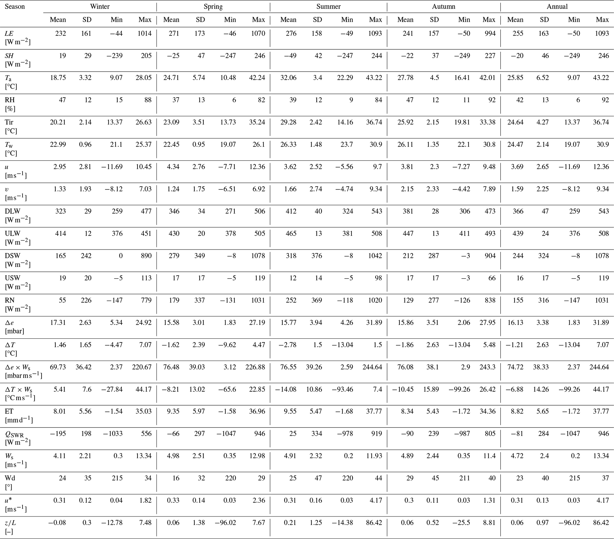
The bulk formula for LE and SH at the GoE underestimates the values (Table 1): during winter, the bulk formula mean (Fig. 5a and c, respectively) values were the closest to the higher EC values. In spring, the difference between the two methods increased, reaching a maximum during summer. The annual maximum of the seasonal mean of the EC measurements was during summer, whereas the bulk formula's was during winter.
Table 1EC and bulk formula seasonal and annual mean LE and SH flux comparison.
The measured 3D anemometer mean friction velocity (0.31 m s−1) was ∼ 2 times larger (Fig. 5b) than the bulk formula estimation from the 2D wind measurement (0.14 m s−1). The ABL stability parameter (ζ) (Fig. 5g) showed a pronounced seasonal variation reaching its minimum value during the winter of ∼ (−12) and maximum value during the summer of ∼ 17, with an overall mean value of −0.04. On the other hand, ζ calculated by the EC system had a much less pronounced variation between the minimum and maximum values in the interval , with a mean value of 0.06. The mean annual derived vapor transfer coefficient, Ce, from the EC LE is 0.00229 (Eq. 9), whereas the bulk formula Ce is 0.00108 (Fig. 5d). However, the bulk formula seasonal means of Ce varied within 2 orders of magnitude, while the EC-derived Ce varied in the scale of 1 order of a magnitude (the seasonal mean range of bulk formula Ce being [0.00064,0.00165] and [0.00186,0.00276] for EC). The difference between the daily mean values of the SH flux calculated by the bulk formula and the EC approach is 20 W m−2.
3.2.5 Seawater residual – net surface heat exchange
The seawater heat gain or loss through the sea surface is defined as the seawater residual heat flux (QSWR), calculated as the sum of the measured surface fluxes LE and SH and RN (i.e., net surface fluxes). The measured QSWR is presented in a diurnal and seasonal diagram in Fig. 2i–k and as a diurnal mean per season in Fig. 3a.
The QSWR mean observation period value was −79 W m−2, which led to a net cooling of the surface water through the surface fluxes. Apart from in summer, the seawater residual was negative, reaching a minimum seasonal mean value of −195 W m−2 during winter and a maximum seasonal mean value of 27 W m−2 in summer. The mean diurnal cycle of the seawater residual was positive through ∼ 08:00–15:00 LT; then, in the afternoon, it was negative for the entire night and early morning. The change from the positive values of seawater residual to negative values in the afternoon coincides with the maximum of the mean daily cycle of the water temperature (Figs. 3 and S4).
3.2.6 The change in the stored heat and seawater residual
Figure 6 presents the available measured heat transfer components of the surface and water-column heat exchange during three campaigns and the advection flux as a residual form of the energy balance equation (Eq. 1). Examining data from three campaigns for calculating GoE heat storage in the top 145 m of surface water showed that in the three campaigns, the deficit required to close the energy heat balance was 74, 88, and 175 W m−2 during winter, summer, and autumn, respectively. During the winter campaign, there was a net cooling of the upper mixed layer of 0–145 m (water-column temperature and salinity ranged from 21.4–22.1 °C and 40.34–40.85 PSU, respectively). The net cooling is equivalent to −83 W m−2 in heat storage change (G). During summer, there was net heating of the strongly stratified water (water-column temperature and salinity ranged from 21.4–28.0 °C and 40.45–40.78 PSU, respectively), which was equivalent to a 95 W m−2 in heat storage change (G). During both campaigns, G did not equal QSWR. During autumn, the G of the mixed top water column was negligible (5 W m−2), and the largest deficit in the heat balance closure exists due to the strong surface cooling ( W m−2).
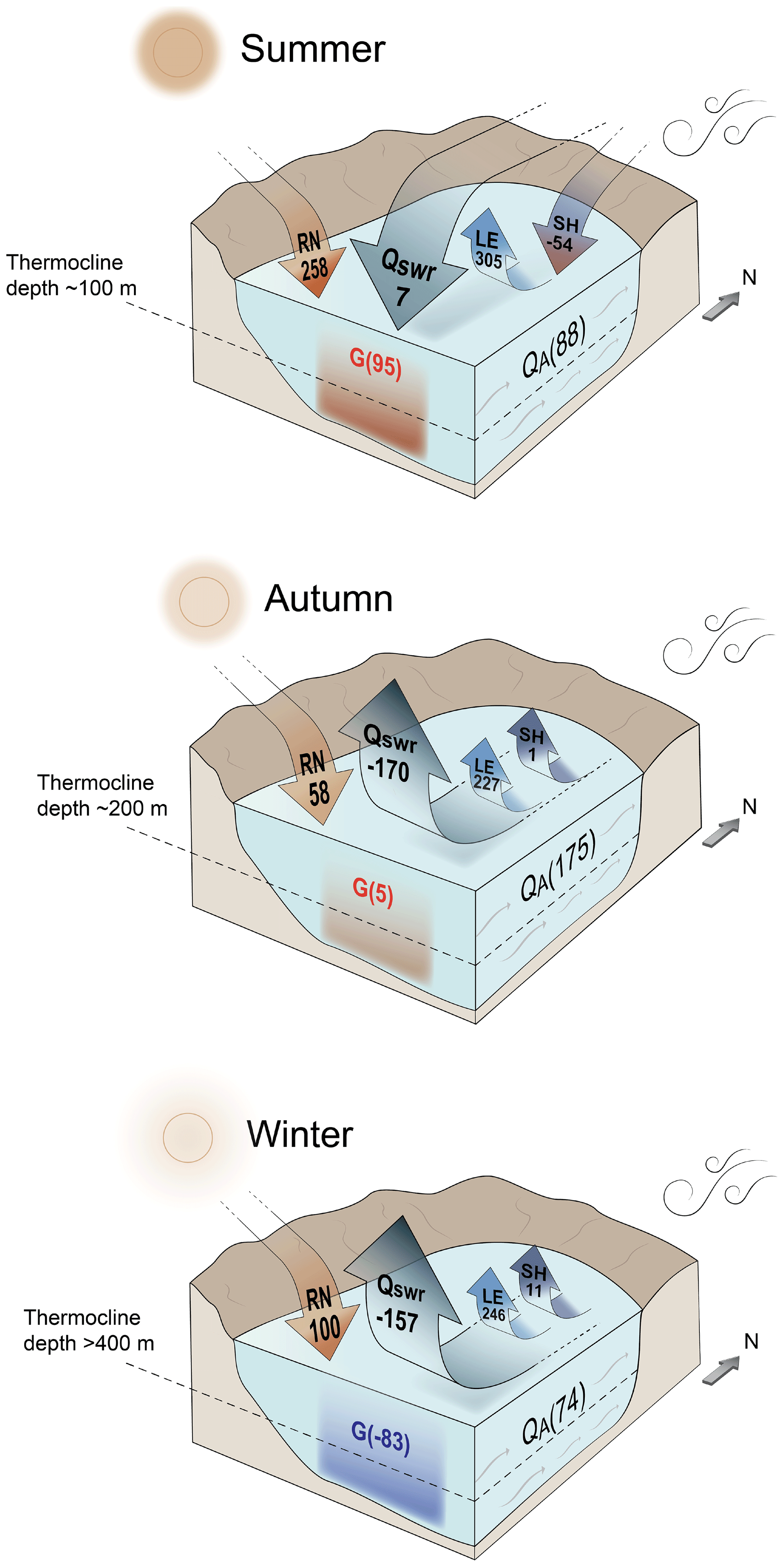
Figure 6Schematic representation of the mean energy partitioning at the GoE during the three campaigns, when water temperature profiles are available (values are given in W m−2).
3.3 Synoptic forced winter heat loss event
We examine here how irregular synoptic-scale forcing events drive intensive heat loss from the water surface to the atmosphere. Over the course of 3 d (25–27 December 2021), intensification of wind speed and cooler and dry air mass forced high rates of heat loss from the sea surface to the atmosphere by LE and SH.
Figure 7 presents the formation and decay of the RST (Alpert et al., 2004) surface-level synoptic state and intensification of the Arabian High, associated with a large surface-water heat loss event. The described synoptic pattern caused an increase in daily mean wind speeds, from 3.8 to 5.9 m s−1 (Fig. 8a), relative to the seasonal mean (DJF 2021–2022). This mean increase also manifested itself as an increase in the minimum and maximum daily wind speed values at the GoE for the 3 d. Surface wind direction at the GoE was northeasterly (23° from the north), with an intensification of the westward component of the wind between 800 and 500 hPa (Fig. S5e) in the region. Additionally, during the event, colder air masses in comparison with the sea temperature were present in the GoE (the ΔT during the event was 1.5 °C higher than the seasonal mean). The increase in Ws and ΔT forced a large heat loss from the surface water of the GoE (Fig. 8i), −270 W m−2 stronger than the DJF mean, which is 1.7 times the standard deviation (SD) of the seasonal mean. The largest mean daily heat loss occurred on 26 December (mean daily value of W m−2), coinciding with the peak of Ws during the event (8.9 m s−1). The surface heat loss is a result of the strong fluxes of LE and SH (Fig. 8f and g, respectively), which increased from 247 to 475 W m−2 (a 2 SD increase from the seasonal mean) and 19 to 44 W m−2 (a 1.25 SD increase from the seasonal mean), respectively. Unlike this event, where the high Ws and mean values of RH and lower Ta (Fig. 8b and c, respectively) resulted in a large heat loss from the surface of the GoE, on 9 January 2022 (shaded yellow area in Fig. 8k), an even higher mean daily wind speed (7.2 m s−1) was measured. However, the mean LE flux measured only 314 W m−2, and SH decreased to 2 W m−2. Contrary to the portrayed heat loss event, on 9 January, warmer and more humid southerly winds persisted (184°). These air mass characteristics resulted in a decrease in Δe and ΔT (Δe=8.5 mbar, ∼ 9 mbar lower than the season and the event mean value; ΔT=0.8 °C), which did not allow for high rates of heat loss in comparison with the seasonal mean. Overall, during the winter season of 2021–2022, there were 7 d where the mean daily QSWR was stronger than −400 W m−2 in comparison with the previous winter of 2020–2021, where only 2 d were recorded (mean winter W m−2). The synoptic pattern of 5 out of 7 of the days in winter 2021–2022 was classified as either RST or high to the east (Arabian High) (see Alpert et al., 2004, for the classification method). Out of the 7 d, two events that prolonged a single day can be identified – the first is a 2 d event and the latter is the prescribed 3 d event; thus, large heat loss occurred mostly through events rather than sporadic heat loss days.
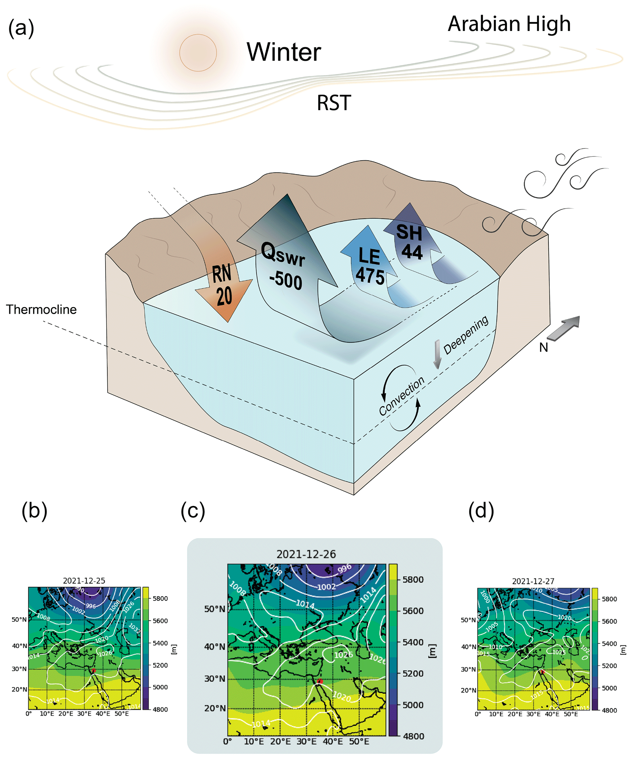
Figure 7(b–d) Surface heat loss case study synoptic maps and (a) a schematic representation of the mean energy partitioning during the event. (b–d) Average daily ERA5 Reanalysis variable synoptic maps; sea level pressure (hPa) is plotted in white contour (Hersbach et al., 2023b), and the 500 hPa geopotential height (m) is plotted in shaded colors (Hersbach et al., 2023a). The event occurred between 25 and 27 December 2021 (the shaded map marks the peak of the event) and involved the intensification of the Arabian High and the Red Sea Trough. (a) Surface energy fluxes are given in W m−2. The large heat loss affects the deepening of the thermocline and the winter annual vertical water-column mixing.
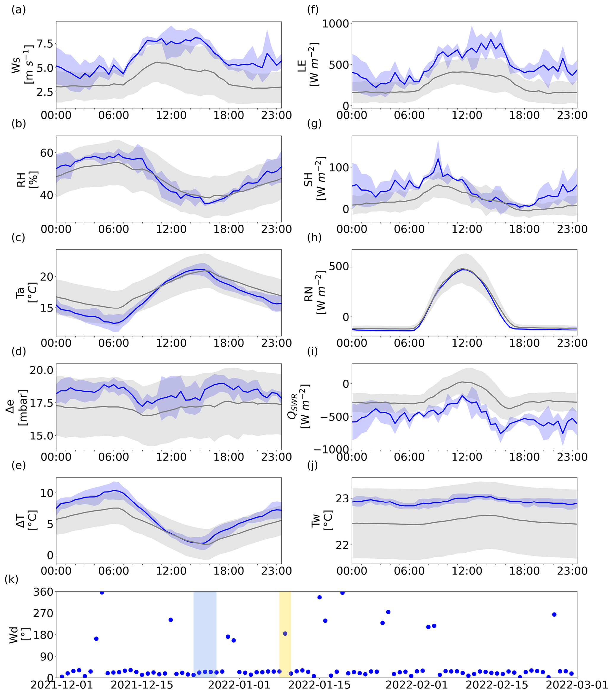
Figure 8 Extreme surface heat loss case study mean diurnal cycle (LT) during the event (blue) and the reference DJF 2021 period (gray); the shaded area is the ± 1 SD span. The panels show (a) wind speed (Ws), (b) relative humidity (RH), (c) air temperature (Ta), (d) vapor pressure difference (Δe), (e) water–air temperature difference (ΔT), (f) latent heat flux (LE), (g) sensible heat flux (SH), (h) net radiation (RN), (i) seawater residual (QSWR), (j) water temperature (Tw), and (k) DJF mean daily wind direction. The blue shaded area marks the heat loss event (25–28 December 2021), and the yellow shaded area is the comparison event (9 January 2022) where the wind is sea-originated; therefore, high air temperature and relative humidity prevent high rates of heat loss.
Accurate quantification of heat and gas exchange between semi-enclosed seas and the atmosphere is essential for understanding the exchange of mass, momentum, and energy within the water column. The GoE, a semi-enclosed sea located in a desert region, is a perfect natural laboratory for studying air–sea interactions in marine environments, where the stable atmospheric boundary layer persists.
4.1 Evaporation rates at the arid semi-enclosed sea: direct measurements vs. bulk formulae
The annual mean evaporation rate of 3.22 m yr−1, presented here, is based on direct measurements and is approximately 2 times larger than earlier estimations based on indirect bulk formulae (Ben-Sasson et al., 2009). Our findings support the product of Ws and Δe as the main forcing mechanism for evaporation in the GoE, in agreement with Lensky et al. (2018) and Tau et al. (2022), with high correlations observed in both diurnal and seasonal timescales. However, in the extremely arid environment of the GoE where Δe is always positive and has high values, evaporation is mostly governed by Ws (correlation of LE with Ws is 0.97 and to Δe×Ws is 0.98). Accordingly, although the mean Δe is higher in winter and the water surface temperature is higher than the overlying air temperature, thus promoting thermal convection, evaporation is higher in summer due to the high wind speed that is sustained longer in the day and the coincidence with the high Δe during the afternoon. Ben-Sasson et al. (2009) estimated higher evaporation during winter based on the bulk formulae approach, which overestimates the role of vertical thermal stability of the air (warmer water underneath the colder air); thus, they predicted that in winter, the free convection due to atmospheric instability led to increased evaporation rates.
The bulk formula estimation of the LE and SH fluxes reproduced similar seasonal trends and values as Ben-Sasson et al. (2009). The comparison with our EC measurements indicated that the bulk formulae are not appropriate for complex desert semi-enclosed seas – specifically, the parametrization of the ABL stability and the calculation of the friction velocity through their relation to the bulk Richardson number, indicated by the large deviation of the stability parameter and the lower friction velocity of the bulk formula in comparison with the EC values. These findings are consistent with the observations of Bardal et al. (2018) regarding the sensitivity of ABL stability to parametrization methods in coastal regions. Proving to be a major caveat, when the stable ABL is calculated using the bulk formula, a lower water vapor transfer coefficient is assigned, resulting in inaccurate lower evaporation rates outside winter. These lower bulk formula evaporation rates occur despite Δe×Ws being higher outside winter, also causing the measured EC evaporation flux to increase outside winter along with Δe×Ws.
The complex nature of the sharp gradients between the arid landscape and sea and the proximity to the mountainous shore presents a challenge for the bulk formulae; it was originally calibrated for the open tropical ocean, where unstable MABL conditions persist and rely on empirical relations. To address this issue, a similar effort in the TOGA COARE campaign (Fairall et al., 1996) is required to refine the bulk formulae parametrization in this intricate environment. The efforts need to focus on the relationship between the easily computed bulk Richardson number and atmospheric stability and friction velocity. Until such efforts are made, we recommend that the direct method of the EC approach be used, as it is the only method with sufficient accuracy for evaporation rate estimation in these settings. These lessons will probably transfer to similar regions such as the Persian Gulf and outside the desert regions, where coastal upwelling and land-originated winds determine a stable ABL over the sea.
The SH flux is small compared to radiation and LE fluxes (−20 W m−2), transferring overall heat from the air to the sea according to the air–sea temperature difference. The bulk formula like in the case of LE underestimates the SH flux.
4.2 Diurnal cycle and water temperature regulation
The diurnal cycle of heat fluxes and micrometeorology shows that from mid-spring to mid-autumn, in the afternoon, the warmer water and the higher air temperature led to reduced RH and consequently to high Δe. This coincides with the diurnal high Ws, which results not only in the daily maximum evaporation rate but also in a double-peak mean diurnal evaporation cycle. Furthermore, this results in higher evaporation after maximum diurnal radiation. This timing of the diurnal maximum in the evaporative cooling effect has critical ramifications for the diurnal thermoregulation processes of shallow water, where coral reefs reside. The diurnal energy partitioning demonstrates how an increase in water temperature is mitigated by evaporative cooling under the normal conditions of sustained daytime winds and extremely dry and hot air. This kind of intense thermoregulation processes can exist in areas where land–sea wind regimes result in persistent dry winds flowing over the surface of the sea.
The strong evaporation enabled by the dry air overcomes the input of energy through the surface of the sea, resulting in a negative QSWR −79 W m−2. Similar to the thermoregulation processes at the coral reef of the GoE (Abir et al., 2022) in the summer under oasis effect conditions of hot dry air above cooler water, the surface fluxes thermoregulate the shallow water temperature at the diurnal timescale. The water temperature reaches its maximum diurnal value shortly after peak radiation, 3 h before the Ta maximum diurnal value. The lag of air temperature behind the water temperature is not intuitive since the heat capacity of water is larger than the air's. This is caused by the strong evaporative cooling effect, as indicated by the coincidence of the maximum daily Tw and the crossing of the QSWR to negative values in the afternoon, emphasizing the effectiveness of QSWR in analyzing daily surface heat balance and thermoregulation processes.
4.3 Energy balance closure and advection term estimation
Throughout most of the 2-year observation period, the surface fluxes cool the surface water. Without the support of advected heat, the evaporation rate decays due to the cooling of the water and decreased water vapor pressure; therefore, this continuous high rate of evaporation can only be sustained with the advection of heat from the south (Biton and Gildor, 2011a).
During the winter, autumn, and summer campaigns, the heat storage was calculated based on temperature measurements of the top 145 m of the GoE. During winter, when several hundred meters (> 400 m; Shaked and Genin, 2022) of the water column is mixed, the deficit to complete the energy balance closure could account for mainly two factors – the cooling of the deeper water column (which was not measured) and heat transported by advection. During autumn, due to the thermocline being deeper than our measurements of temperature (∼ 200 m; Shaked and Genin, 2022), the large deficit to the energy balance closure (174 W m−2) is attributed to advection through the northern-bound surface currents, cooling of the deeper water, and deepening of the thermocline. During summer, when the shallow water is strongly stratified, the thermocline is ∼ 100 m deep, and the net surface fluxes are relatively weak (7 W m−2), the warming of the water is a direct result of heat advection from the south as Biton and Gildor (2011b) found. Therefore, we conclude that the surface fluxes contribute to the heating processes of the surface water only at the diurnal scale and offer substantial cooling during the seasonal timescale.
4.4 Winter synoptic-scale forcing for high rates of heat loss
We demonstrate how wintertime synoptic-scale variability in atmospheric circulation drives extreme rates of heat loss from the water of the GoE. Our direct flux measurements resolved the gap from previous studies that utilized remote sensing data with a larger pixel size than the GoE width (Menezes et al., 2019; Papadopoulos et al., 2013). The steep sea level pressure gradient over the Red Sea, caused by the low-pressure system, resulted in high wind speeds, which are cold and dry (land originated wind), leading to high rates of heat loss during winter. The cooling of the surface water by the daily mean rate of ∼ −500 W m−2 during the event, which is 2.5 times larger than the 2-year winter mean, increased the density of the surface water by increasing salinity through evaporation and by cooling. Thus, the cooling event impacted the vertical stability of the water column and enhanced processes that led to the annual winter vertical mixing processes. Indeed, the water column at the northern GoE was mixed during that winter (2021–2022) to a depth greater than 700 m for the first time in a decade, where the mixing depth did not exceed ∼ 500 m, additionally supported by the number of large heat loss events during the winter (especially during December), before the deep mixing year and the shallow depth mixing year in our observation period (> 700 and 450 m, respectively). This relation of extreme surface heat losses, driven by synoptic-scale circulation, to winter water-column mixing (basin overturning circulation) should be further explored as a preconditioning event for winter water-column mixing along with how the surface fluxes change with response to winds traversing longer distances over the narrow sea.
Over a 2-year period, direct measurements in the Gulf of Eilat (GoE), a locked sea in a hyper-arid region, reveal a significantly higher annual mean evaporation rate (3.22 m yr−1) compared to lower indirect estimates using bulk formulae (1.6–1.8 m yr−1). The minimum evaporation rate was measured during the winter season, due to the lowest wind speed therein and vapor pressure difference. Previous indirect estimations revealed that evaporation was the highest during winter due to the highest thermal instability of the ABL.
Higher evaporation rates during the warmer seasons, spring, summer, and autumn, are attributed to increased wind speed persisting into the evening, particularly in the afternoon. This aligns temporally with the diurnal maximum in vapor pressure difference, resulting from decreased relative humidity and surface-water warming. The seasonal wind speed trend was found to be stronger than the seasonal vapor pressure difference trend in determining the seasonal evaporation rate in arid regions.
The current parametrization of bulk formulae vapor transfer coefficient exhibits uncertainties, particularly in stable atmospheric boundary layer (ABL) environments. Our findings underscore the need to revisit ABL stability parametrization and friction velocity calculation, especially in environments where warm air travels over cooler water. The derived vapor transfer coefficient from eddy covariance (EC) measurements is 0.00229, which is applicable to the northern GoE.
Surface energy exchange fluxes predominantly cool surface water, with minimal heating through the surface fluxes during summer, which is insufficient for explaining the annual temperature increase in warm seasons. Advection fluxes, bringing warmer water to the GoE, sustain high evaporation rates year-round. Winter synoptic-scale events forcing high surface heat and moisture loss from the sea may precondition deep vertical water-column mixing in the GoE.
Accurate evaporation estimates are crucial for ocean circulation modeling, both for base-state and acute-event modeling, requiring an update of ocean dynamics simulations based on the new understanding of air–sea interactions in these environments.
We emphasize the need for future efforts in resolving the spatial distribution of the evaporation rate, ABL stability, and surface friction velocity at the GoE, Red Sea, and other coastal areas.
Table A1Seasonal mean and the entire observation period statistics of micrometeorological and flux variables.
Datasets for this research are available from Abir et al. (2023, https://doi.org/10.17632/wmtdmjgsfp.1).
The IUI monitoring program data used for this research are available at http://www.meteo-tech.co.il/eilat-yam/eilat_en.asp (Gulf of Eilat Meteorological Station, 2024). The Wirewalker CTD data are available upon request from Hezi Gildor (hezi.gildor@mail.huj.ac.il).
The ERA5 hourly data at a single level (Hersbach et al., 2023b) and pressure level (Hersbach et al., 2023a, https://doi.org/10.24381/cds.68d2bb30) in this study are available online.
Software for this research is available from LI-COR Biosciences (2021), available at https://www.licor.com/env/support/EddyPro/software.html.
The supplement related to this article is available online at: https://doi.org/10.5194/acp-24-6177-2024-supplement.
The study was conceptualized by SA, NGL, and HAM. Data curation was carried out by SA, with NGL, HG, and YS. Formal analysis, investigation, software, and visualization were done by SA, under supervision of NGL. Writing the original draft was done by SA, under the supervision of NGL, and revisions were made by EM, HAM, HG, and YS. The review and editing of the manuscript were done by SA, who was assisted by NGL, HAM, HG, and EM.
The contact author has declared that none of the authors has any competing interests.
Publisher's note: Copernicus Publications remains neutral with regard to jurisdictional claims made in the text, published maps, institutional affiliations, or any other geographical representation in this paper. While Copernicus Publications makes every effort to include appropriate place names, the final responsibility lies with the authors.
We thank the team from the Geological Survey of Israel – Uri Malik, Guy Tau, and Ziv Mor. We also thank Yoav Balaban for the graphic illustration; Asaph Rivlin, Modi Pilersdorf, the Israel National Monitoring Program at the Gulf of Eilat, and the Interuniversity Institute for Marine Sciences in Eilat for access to infrastructure and services; and Assaf Zvuloni and Chen Toufikian of Israel's Nature and Parks Authority for their assistance. We thank Pinhas Alpert and the Hadas Saaroni lab for giving us access to their daily synoptic classification dataset.
The research was supported by the Israel Science Foundation with a grant (grant no. ISF-2018/1471) awarded to principal investigator (PI) Nadav G. Lensky and by funds for PIs Efrat Morin, Hamish A. McGowan, and Nadav G. Lensky from the Hebrew University of Jerusalem–Zelman Cowen Academic Initiatives (ZCAI) Joint Projects 2021 (2022–2024). Hezi Gildor was supported by a grant from the Ministry of Science and Technology of Israel. The University of Queensland financially and technically supported the research.
This paper was edited by Ashu Dastoor and reviewed by three anonymous referees.
Abir, S., McGowan, H. A., Shaked, Y., and Lensky, N. G.: Identifying an Evaporative Thermal Refugium for the Preservation of Coral Reefs in a Warming World – The Gulf of Eilat (Aqaba), J. Geophys. Res-Atmos., 127, e2022JD036845, https://doi.org/10.1029/2022JD036845, 2022.
Abir, S., McGowan, H., Shaked, Y., Morin, E., and Lensky, N.: 2 years Eddy Covariance measurements over the Gulf of Eilat (Aqaba), V1, Mendeley data [data set], https://doi.org/10.17632/wmtdmjgsfp.1, 2023.
Afargan, H. and Gildor, H.: The role of the wind in the formation of coherent eddies in the Gulf of Eilat/Aqaba, J. Marine Syst., 142, 75–95, https://doi.org/10.1016/j.jmarsys.2014.09.006, 2015.
Allouche, M., Bou-Zeid, E., and Iipponen, J.: The influence of synoptic wind on land–sea breezes, Q. J. Roy. Meteor. Soc., 149, 3198–3219, https://doi.org/10.1002/qj.4552, 2023.
Alpert, P., Osetinsky, I., Ziv, B., and Shafir, H.: Semi-objective classification for daily synoptic systems: Application to the eastern Mediterranean climate change, Int. J. Climatol., 24, 1001–1011, https://doi.org/10.1002/joc.1036, 2004.
Assaf, G. and Kessler, J.: Climate and energy exchange in the Gulf of Aqaba (Eilat), Mon. Weather Rev., 104, 381–385, 1976.
Azorin-Molina, C. and Chen, D.: A climatological study of the influence of synoptic-scale flows on sea breeze evolution in the Bay of Alicante (Spain), Theor. Appl. Climatol., 96, 249–260, https://doi.org/10.1007/s00704-008-0028-2, 2009.
Bardal, L. M., Onstad, A. E., Sætran, L. R., and Lund, J. A.: Evaluation of methods for estimating atmospheric stability at two coastal sites, Wind Engineering, 42, 561–575, https://doi.org/10.1177/0309524X18780378, 2018.
Ben-Sasson, M., Brenner, S., and Paldor, N.: Estimating air-sea heat fluxes in semienclosed basins: The case of the Gulf of Elat (Aqaba), J. Phys. Oceanogr., 39, 185–202, https://doi.org/10.1175/2008JPO3858.1, 2009.
Berman, T., Paldor, N., and Brenner, S.: Simulation of wind-driven circulation in the Gulf of Elat Aqaba, J. Marine Syst., 26, 349–365, 2000.
Berman, T., Paldor, N., and Brenner, S.: The seasonality of tidal circulation in the Gulf of Elat, Israel J. Earth Sci., 52, 11–19, 2003.
Bignami, F., Marullo, S., Santoleri, R., and Schiano, M. E.: Longwave radiation budget in the Mediterranean Sea, J. Geophys. Res., 100, 2501–2514, https://doi.org/10.1029/94JC02496, 1995.
Biton, E. and Gildor, H.: Stepwise seasonal restratification and the evolution of salinity minimum in the Gulf of Aqaba (Gulf of Eilat), J. Geophys. Res.-Oceans, 116, C08022, https://doi.org/10.1029/2011JC007106, 2011a.
Biton, E. and Gildor, H.: The general circulation of the Gulf of Aqaba (Gulf of Eilat) revisited: The interplay between the exchange flow through the Straits of Tiran and surface fluxes, J. Geophys. Res.-Oceans, 116, C08020, https://doi.org/10.1029/2010JC006860, 2011b.
Dayan, U., Tubi, A., and Levy, I.: On the importance of synoptic classification methods with respect to environmental phenomena, Int. J. Climatol., 32, 681–694, https://doi.org/10.1002/joc.2297, 2012.
EddyPro 7 Software: Express default settings, https://www.licor.com/env/support/EddyPro/topics/express-defaults.html, last access: 13 June 2023.
Edson, J., Crawford, T., Crescenti, J., Farrar, T., Frew, N., Gerbi, G., Helmis, C., Hristov, T., Khelif, D., Jessup, A., Jonsson, H., Li, M., Mahrt, L., McGillis, W., Plueddemann, A., Shen, L., Skyllingstad, E., Stanton, T., Sullivan, P., Sun, J., Trowbridge, J., Vickers, D., Wang, S., Wang, Q., Weller, R., Wilkin, J., Williams III, A. J., Yue, D. K. P., and Zappa, C.: The Coupled Boundary Layers and Air–Sea Transfer Experiment in Low Winds, B. Am. Meteorol. Soc., 88, 341–356, https://doi.org/10.1175/BAMS-88-3-341, 2007.
Eshel, G. and Heavens, N.: Climatological evaporation seasonality in the northern Red Sea, Paleoceanography, 22, PA4201, https://doi.org/10.1029/2006PA001365, 2007.
Fairall, C. W., Bradley, E. F., Rogers, D. P., Edson, J. B., and Young, G. S.: Bulk parameterization of air-sea fluxes for tropical ocean-global atmosphere coupled-ocean atmosphere response experiment, J. Geophys. Res.-Oceans, 101, 3747–3764, https://doi.org/10.1029/95JC03205, 1996.
Fine, M., Gildor, H., and Genin, A.: A coral reef refuge in the Red Sea, Glob. Change Biol., 19, 3640–3647, 2013.
Foken, T., Göckede, M., Mauder, M., Mahrt, L., Amiro, B., and Munger, W.: Hand book of Micromereotology post-field data quality control, in: Handbook of Micrometeorology. Atmospheric and Oceanographic Sciences Library, edited by: Lee, X., Massman, W., Law, B., Vol. 29, 181–208, Springer, Dordrecht, https://doi.org/10.1007/1-4020-2265-4_9, 2004.
Genin, A., Levy, L., Sharon, G., Raitsos, E. D. E., and Diamant, A.: Rapid onsets of warming events trigger mass mortality of coral reef fish, P. Natl. Acad. Sci. USA, https://doi.org/10.1073/pnas.2009748117, 2020.
Gulf of Eilat (NMP) Meteorological Station: IUI monitoring program data, Meteo-tech [data set], http://www.meteo-tech.co.il/eilat-yam/eilat_en.asp, last access: 25 May 2024.
Gutiérrez-Loza, L. and Ocampo-Torres, F. J.: Air-sea CO2 fluxes measured by eddy covariance in a coastal station in Baja California, México, IOP Conference Series: Earth and Environmental Science, 35, 012012, https://doi.org/10.1088/1755-1315/35/1/012012, 2016.
Hamdani, I., Assouline, S., Tanny, J., Lensky, I. M., Gertman, I., Mor, Z., and Lensky, N. G.: Seasonal and diurnal evaporation from a deep hypersaline lake: The Dead Sea as a case study, J. Hydrol., 562, 155–167, https://doi.org/10.1016/j.jhydrol.2018.04.057, 2018.
Hersbach, H., Bell, B., Berrisford, P., Biavati, G., Horányi, A., Muñoz Sabater, J., Nicolas, J., Peubey, C., Radu, R., Rozum, I., Schepers, D., Simmons, A., Soci, C., Dee, D., and Thépaut, J.-N.: ERA5 hourly data on pressure levels from 1940 to present, CDS [data set], https://doi.org/10.24381/cds.68d2bb30, 2023a.
Hersbach, H., Bell, B., Berrisford, P., Biavati, G., Horányi, A., Muñoz Sabater, J., Nicolas, J., Peubey, C., Radu, R., Rozum, I., Schepers, D., Simmons, A., Soci, C., Dee, D., and Thépaut, J.-N.: ERA5 hourly data on single levels from 1940 to present, CDS [data set], https://doi.org/10.24381/cds.adbb2d47, 2023b.
Hsieh, C.-I., Katul, G., and Chi, T.: An approximate analytical model for footprint estimation of scalar fluxes in thermally stratified atmospheric flows, Adv. Water Resour., 23, 765–772, 2000.
Klinker, J., Reiss, Z., Kropach, C., Levanon, I., Harpaz, H., Halicz, E., and Assaf, G.: Observations on the Circulation Pattern in the Gulf of Elat (Aqaba), Red Sea, Israel J. Earth Sci., 25, 85–103, 1976.
Kljun, N., Calanca, P., Rotach, M. W., and Schmid, H. P.: A simple parameterisation for flux footprint predictions, Bound.-Lay. Meteorol., 112, 503–523, 2004.
Kondo, J.: Air-sea Bulk Transfer Coefficient in Diabatic Conditions, Bound.-Lay. Meteorol., 9, 91–112, https://doi.org/10.1007/BF00232256, 1975.
Kormann, R. and Meixner, F. X.: An analytical footprint model for nonneutral stratification, Bound.-Lay. Meteorol., 99, 207–224, 2001.
Lensky, N. G., Lensky, I. M., Peretz, A., Gertman, I., Tanny, J., and Assouline, S.: Diurnal Course of Evaporation From the Dead Sea in Summer: A Distinct Double Peak Induced by Solar Radiation and Night Sea Breeze, Water Resour. Res., 54, 150–160, https://doi.org/10.1002/2017WR021536, 2018.
LI-COR Biosciences: EddyPro Software v7.0, https://www.licor.com/env/support/EddyPro/software.html (last access: 25 May 2024), 2021.
MacKellar, M. C. and McGowan, H.: Air-sea energy exchanges measured by eddy covariance during a localised coral bleaching event, Heron Reef, Great Barrier Reef, Australia, Geophys. Res. Lett., 37, L24703, https://doi.org/10.1029/2010GL045291, 2010.
Mahabbati, A., Beringer, J., Leopold, M., McHugh, I., Cleverly, J., Isaac, P., and Izady, A.: A comparison of gap-filling algorithms for eddy covariance fluxes and their drivers, Geosci. Instrum. Method. Data Syst., 10, 123–140, https://doi.org/10.5194/gi-10-123-2021, 2021.
McGowan, H., Sturman, A. P., MacKellar, M. C., Wiebe, A. H., and Neil, D. T.: Measurements of the local energy balance over a coral reef flat, Heron Island, southern Great Barrier Reef, Australia, J. Geophys. Res.-Atmos., 115, D19124, https://doi.org/10.1029/2010JD014218, 2010.
McGowan, H., Sturman, A., Saunders, M., Theobald, A., and Wiebe, A.: Insights From a Decade of Research on Coral Reef – Atmosphere Energetics, J. Geophys. Res.-Atmos., 124, 4269–4282, https://doi.org/10.1029/2018JD029830, 2019.
Menezes, V. V., Farrar, J. T., and Bower, A. S.: Evaporative Implications of Dry-Air Outbreaks Over the Northern Red Sea, J. Geophys. Res.-Atmos., 124, 4829–4861, https://doi.org/10.1029/2018JD028853, 2019.
Meteorological Service: Eilat annual average precipitation, Meteorological Service [data set], https://ims.gov.il/he/ClimateAtlas, last access: 13 June 2023.
Mor, Z., Assouline, S., Tanny, J., Lensky, I. M., and Lensky, N. G.: Effect of Water Surface Salinity on Evaporation: The Case of a Diluted Buoyant Plume Over the Dead Sea, Water Resour. Res., 54, 1460–1475, https://doi.org/10.1002/2017WR021995, 2018.
Morin, T. H., Bohrer, G., Naor-Azrieli, L., Mesi, S., Kenny, W. T., Mitsch, W. J., and Schäfer, K. V. R.: The seasonal and diurnal dynamics of methane flux at a created urban wetland, Ecol. Eng., 72, 74–83, https://doi.org/10.1016/j.ecoleng.2014.02.002, 2014.
Papadopoulos, V. P., Abualnaja, Y., Josey, S. A., Bower, A., Raitsos, D. E., Kontoyiannis, H., and Hoteit, I.: Atmospheric forcing of the winter air-sea heat fluxes over the northern red sea, J. Climate, 26, 1685–1701, https://doi.org/10.1175/JCLI-D-12-00267.1, 2013.
Paynes, R. E.: Albedo of the sea surface, J. Atmos. Sci., 29, 959–970, https://doi.org/10.1175/1520-0469(1972)029<0959:AOTSS>2.0.CO;2, 1972.
Pérez, A., Lagos, O., Lillo-Saavedra, M., Souto, C., Paredes, J., and Arumí, J. L.: Mountain lake evaporation: A comparative study between hourly estimations models and in situ measurements, Water-Sui, 12, 2648, https://doi.org/10.3390/w12092648, 2020.
Pivato, M., Carniello, L., Gardner, J., Silvestri, S., and Marani, M.: Water and sediment temperature dynamics in shallow tidal environments: The role of the heat flux at the sediment-water interface, Adv. Water Resour., 113, 126–140, https://doi.org/10.1016/j.advwatres.2018.01.009, 2018.
Rey-Sánchez, A. C., Bohrer, G., Morin, T. H., Shlomo, D., Mirfenderesgi, G., Gildor, H., and Genin, A.: Evaporation and CO2 fluxes in a coastal reef: an eddy covariance approach, Ecosys. Health Sust., 3, 1392830, https://doi.org/10.1080/20964129.2017.1392830, 2017.
Shaked, Y. and Genin, A. (Eds.): Scientific report 2021, Interuniversity Institute for Marine Sciences, Eilat, Israel, https://iui-eilat.ac.il/uploaded/NMP/reports/NMP Report 2021.pdf (last access: 25 May 2024) 2022.
Shalev, E., Lyakhovsky, V., Weinstein, Y., and Ben-Avraham, Z.: The thermal structure of Israel and the Dead Sea Fault, Tectonophysics, 602, 69–77, https://doi.org/10.1016/j.tecto.2012.09.011, 2013.
Sofianos, S. S., Johns, W. E., and Murray, S. P.: Heat and freshwater budgets in the Red Sea from direct observations at Bab el Mandeb, Deep-Sea Res. Pt. II, 49, 1323–1340, https://doi.org/10.1016/S0967-0645(01)00164-3, 2002.
Sverdrup, H. U., Johnson, M. W., and Fleming, R. H.: The Oceans, Their Physics, Chemistry, and General Biology, Prentice-Hall, New York, http://ark.cdlib.org/ark:/13030/kt167nb66r/ (last access: 25 May 2024), 1942.
Tau, G., Enzel, Y., McGowan, H., Lyakhovsky, V., and Lensky, N. G.: Air-water interactions regulating water temperature of lakes: Direct observations (Agamon Hula, Israel) and analytical solutions, J. Hydrol., 614, 128515, https://doi.org/10.1016/J.JHYDROL.2022.128515, 2022.
Yu, L.: Global Air-Sea Fluxes of Heat, Fresh Water, and Momentum: Energy Budget Closure and Unanswered Questions, Annu. Rev. Mar. Sci., 11, 227–248, https://doi.org/10.1146/annurev-marine-010816-060704, 2018.