Surface snow bromide and nitrate at Eureka, Canada, in early spring and implications for polar boundary layer chemistry

This study explores the role of snowpack in polar boundary layer chemistry, especially as a direct source of reactive bromine (BrO_x = BrO + Br) and nitrogen (NO_x = NO + NO₂) in the Arctic springtime. Surface snow samples were collected daily from a Canadian high Arctic location at Eureka, Nunavut (80° N, 86° W) from the end of February to the end of March in 2018 and 2019. The snow was sampled at several sites representing distinct environments: sea ice, inland close to sea level, and a hilltop ∼ 600 m above sea level ($\mathrm{a}.\mathrm{s}.\mathrm{l}.$). At the inland sites, surface snow salinity has a double-peak distribution with the first and lowest peak at 0.001–0.002 practical salinity unit (psu), which corresponds to the precipitation effect, and the second peak at 0.01–0.04 psu, which is likely related to the salt accumulation effect (due to loss of water vapour by sublimation). Snow salinity on sea ice has a triple-peak distribution; its first and second peaks overlap with the inland peaks, and the third peak at 0.2–0.4 psu is likely due to the sea water effect (a result of upward migration of brine).

At all sites, snow sodium and chloride concentrations increase by almost 10-fold from the top 0.2 to ∼ 1.5 cm. Surface snow bromide at sea level is significantly enriched, indicating a net sink of atmospheric bromine. Moreover, surface snow bromide at sea level has an increasing trend over the measurement period, with mean slopes of 0.024 µM d⁻¹ in the 0–0.2 cm layer and 0.016 µM d⁻¹ in the 0.2–0.5 cm layer. Surface snow nitrate at sea level also shows a significant increasing trend, with mean slopes of 0.27, 0.20, and 0.07 µM d⁻¹ in the top 0.2, 0.2–0.5, and 0.5–1.5 cm layers, respectively. Using these trends, an integrated net deposition flux of bromide of (1.01 ± 0.48) × 10⁷ $\mathrm{molec}.{\mathrm{cm}}^{-\mathrm{2}}{\mathrm{s}}^{-\mathrm{1}}$ and an integrated net deposition flux of nitrate of (2.6 ± 0.37) × 10⁸ $\mathrm{molec}.{\mathrm{cm}}^{-\mathrm{2}}{\mathrm{s}}^{-\mathrm{1}}$ were derived. In addition, the surface snow nitrate and bromide at inland sites were found to be significantly correlated (R = 0.48–0.76) with the $\left[{\mathrm{NO}}_{\mathrm{3}}^{-}\right]/\left[{\mathrm{Br}}^{-}\right]$ ratio of 4–7 indicating a possible acceleration effect of reactive bromine in atmospheric NO_x-to-nitrate conversion. This is the first time such an effect has been seen in snow chemistry data obtained with a sampling frequency as short as 1 d.

BrO partial column (0–4 km) data measured by MAX-DOAS show a decreasing trend in early spring, which generally agrees with the derived surface snow bromide deposition flux indicating that bromine in Eureka atmosphere and surface snow did not reach a photochemical equilibrium state. Through mass balance analysis, we conclude that the average release flux of reactive bromine from snow over the campaign period must be smaller than the derived bromide deposition flux of ∼ 1 × 10⁷ $\mathrm{molec}.{\mathrm{cm}}^{-\mathrm{2}}{\mathrm{s}}^{-\mathrm{1}}$. Note that the net mean fluxes observed do not completely rule out larger bidirectional fluxes over shorter timescales.

1 Introduction

Reactive bromine (BrO_x = BrO + Br) and reactive nitrogen (NO_x = NO + NO₂) are two important families in atmospheric chemistry, both of which play a critical role in determining the oxidizing capacity of the polar boundary layer (Morin et al., 2008). However, the processes involved in the sources, sinks, and recycling of reactive bromine and nitrogen in the air–snow–sea ice system are not fully understood (Abbatt et al., 2012) or parameterized, which prevents quantification of their effects and the ability to make robust predictions for the changing climate using numerical chemical models.

Reactive nitrogen-rich air observed in the Arctic troposphere is mainly anthropogenic and subject to long-range transport (Dickerson, 1985). During winter, gaseous nitric acid (HNO₃) or particulate bond nitrate (p-NO₃) is removed from the air via dry and wet deposition. HNO₃ and p-NO₃ mainly dissolve to form nitrate (${\mathrm{NO}}_{\mathrm{3}}^{-}$) upon contact with the snow cover (Diehl et al., 1995; Abbatt, 1997). Nitrate that accumulates in the snowpack can release gaseous NO_x and HONO in spring via photolysis (Dubowski et al., 2001; Honrath et al., 2002), with the processes controlled by many factors including meteorological parameters and chemical, optical, and physical snow properties. These include photolabile ${\mathrm{NO}}_{\mathrm{3}}^{-}$ concentrations, the amount of light-absorbing impurities, the temperature-dependent quantum yields of ${\mathrm{NO}}_{\mathrm{3}}^{-}$ photolysis, and the timing of precipitation (Beine et al., 2003; Frey et al., 2013; Chan et al., 2015; Zatko et al., 2016; Winton et al., 2020). The measured snow–NO_x emission fluxes in polar regions vary from site to site, ranging from near zero to > 1.0 × 10⁹ $\mathrm{molec}.{\mathrm{cm}}^{-\mathrm{2}}{\mathrm{s}}^{-\mathrm{1}}$ (Jones et al., 2001; Zhou et al., 2001; Honrath et al., 2002; Beine et al., 2002; 2003; Oncley et al., 2004; Frey et al., 2013; Chan et al., 2018). A direct measurement of nitrate dry deposition flux was made by Björkman et al. (2013) in Svalbard using a tray sampling approach. They reported a total flux of 10.27 ± 3.84 mg m⁻² (September 2009 to May 2010), which is roughly equivalent to a mean flux of 4 × 10⁸ $\mathrm{molec}.{\mathrm{cm}}^{-\mathrm{2}}{\mathrm{s}}^{-\mathrm{1}}$. In addition, at Svalbard, precipitation dominates nitrate supply to snow, with dry deposited HNO₃ only accounting for 10 %–14 % of total nitrate (Beine et al., 2003; Björkman et al., 2013).

Observations show that sea-ice regions have the highest tropospheric bromine oxide (BrO) loading on Earth (Wagner and Platt, 1998). BrO enhancements are normally observed in the polar boundary layer during springtime and are referred to as “bromine explosion” events (BEEs). It is well known that saline substrates are the eventual source of reactive bromine (Wagner and Platt, 1998; Oum et al., 1998; Simpson et al., 2007a). Salts may be supplied to the snow surface by upward migration from sea ice, by frost flowers being wind-blown to the snow surface, or by wind-transported aerosols generated by sea spray (Domine et al., 2004). However, the dominant source bromine and the underlying processes involved remain unclear, with more than half a dozen different candidates proposed. These include frost flowers (Kaleschke et al., 2004; Piot and von Glasow, 2008), first-year sea ice surface (Simpson et al., 2005; 2007b), open leads/polynyas (e.g. Peterson et al., 2016; Kirpes et al., 2019; Criscitiello et al., 2021), snowpack on tundra (Pratt et al., 2013), snowpack on sea ice (Custard et al., 2017; Peterson et al., 2019), snowpack on ice sheets (Thomas et al., 2011), and sea salt aerosols from blowing snow (Yang et al., 2008, 2010, 2019, 2020; Frey et al., 2020; Huang et al., 2020). Significant progress has been made in recent decades, with data showing that frost flowers and open leads are only of minor or local importance (Domine et al., 2005; Obbard et al., 2009; Huang et al., 2020). In addition, the proposed stratospheric BrO intrusion (Salawitch et al., 2010) has also been found to be less important than previously thought (Theys et al., 2011). Currently, the major debate surrounds the relative importance of the two remaining candidates – snowpack and blowing snow (e.g. Bognar et al., 2020; Marelle et al., 2021; Swanson et al., 2022).

Reactive bromine can directly cause polar boundary layer ozone depletion events (ODEs), whereby near-surface ozone concentrations in spring drop below 10 ppbv (part per billion by volume), reaching close to 0 ppbv in some cases (Bottenheim et al., 1986; Barrie et al., 1988; Tarasick and Bottenheim, 2002; Jacobi et al., 2012). In addition, BrO_x can affect reactive nitrogen (Morin et al., 2008) and hydroxyl radicals (HO_x = OH + HO₂) (Bloss et al., 2007, 2010; Brough et al., 2019) as well as elemental mercury oxidation (e.g. Holmes et al., 2006; Parella et al., 2012; Angot et al., 2016; Xu et al., 2016; Wang et al., 2019) and dimethyl sulfide oxidation (Hoffmann et al., 2016).

It is well-known that BrO_x can directly react with NO_x via Reactions (R1) and (R2):

$$\begin{array}{}\text{(R1)}& {\displaystyle }& {\displaystyle }\mathrm{BrO}\left(\mathrm{g}\right)+{\mathrm{NO}}_{\mathrm{2}}\left(\mathrm{g}\right)\to {\mathrm{BrONO}}_{\mathrm{2}}\left(\mathrm{g}\right)\text{(R2)}& {\displaystyle }& {\displaystyle }{\mathrm{BrONO}}_{\mathrm{2}}\left(\mathrm{g}\right)+{\mathrm{H}}_{\mathrm{2}}\mathrm{O}\left(\mathrm{aq}\right)\to {\mathrm{HNO}}_{\mathrm{3}}\left(\mathrm{g}\right)+\mathrm{HOBr}\left(\mathrm{g}\right).\end{array}$$

The product HOBr in Reaction (R2) can photolyse to reform Br atoms (Reaction R3) which then react with ozone to form BrO (Reaction R4) to further oxidize NO_x in R1.

$$\begin{array}{}\text{(R3)}& {\displaystyle }& {\displaystyle }\mathrm{HOBr}\left(\mathrm{g}\right)+h\mathit{\nu }\to \mathrm{Br}\left(\mathrm{g}\right)+\mathrm{OH}\left(\mathrm{g}\right)\text{(R4)}& {\displaystyle }& {\displaystyle }\mathrm{Br}\left(\mathrm{g}\right)+{\mathrm{O}}_{\mathrm{3}}\left(\mathrm{g}\right)\to \mathrm{BrO}\left(\mathrm{g}\right)+{\mathrm{O}}_{\mathrm{2}}\left(\mathrm{g}\right)\end{array}$$

Therefore, the net reaction of Reactions (R1)–(R4) is

$$\begin{array}{}\text{(R5)}& {\mathrm{NO}}_{\mathrm{2}}\left(\mathrm{g}\right)+{\mathrm{O}}_{\mathrm{3}}\left(\mathrm{g}\right)+{\mathrm{H}}_{\mathrm{2}}\mathrm{O}\left(\mathrm{aq}\right)+h\mathit{\nu }\to {\mathrm{HNO}}_{\mathrm{3}}\left(\mathrm{g}\right)+{\mathrm{O}}_{\mathrm{2}}\left(\mathrm{g}\right).\end{array}$$

This means that under sunlight and in the presence of bromine, ozone and NO_x molecules will be consumed effectively via chain reactions. Thus, the presence of BrO_x may accelerate the conversion from NO_x to nitrate and influence the atmospheric nitrogen budget. Previous modelling work has estimated that bromine chemistry can cause NO_x reductions of 60 %–80 % at high latitudes in spring (Yang et al., 2005).

The emission fluxes of reactive bromine from blowing snow are all based on parameterization in models (Yang et al., 2008, 2010, 2020; Huang et al., 2020; Swanson et al., 2020; Marelle et al., 2021). There are currently no direct measurements of bromine emission flux from blowing snow. Regarding snowpack bromine emission, a direct gradient measurement of Br₂ and BrCl above a patch of snowpack was made near Utqiaġvik, Alaska, by Custard et al. (2017), who reported emission fluxes of 0.7–12 × 10⁸ $\mathrm{molec}.{\mathrm{cm}}^{-\mathrm{2}}{\mathrm{s}}^{-\mathrm{1}}$. However, their emission fluxes were based on a field dataset obtained over only a few days. Model emission schemes estimate reactive bromine emission fluxes of 9.0 × 10⁷ to 2.7 × 10⁹ $\mathrm{molec}.{\mathrm{cm}}^{-\mathrm{2}}{\mathrm{s}}^{-\mathrm{1}}$, and the emission flux is highly dependent on the parameters applied (Lehrer et al., 2004; Poit and Glasow, 2009; Toyota et al., 2014; Falk and Sinnhuber, 2018; Marelle et al., 2021). The removal of inorganic bromine species (such as HBr, HOBr, Br₂, BrCl, BrONO₂ and BrO) from the atmosphere via wet and dry deposition is mainly calculated by models (e.g. Yang et al., 2005, 2010; Parela et al., 2012; Legrand et al., 2016); thus far, field deposition flux has not been reported.

Both nitrate and bromide undergo post-depositional processes within the snowpack (via photochemistry), and the observationally derived flux represents the net direction of emission and deposition. However, these two processes may occur at different times and at different depths with different rates. For example, the deposited bromide and nitrate may be largely confined to the top few-centimetre layer, while photochemistry may occur only in daytime and across a deep depth (depending on the e-folding depth; Domine et al., 2008).

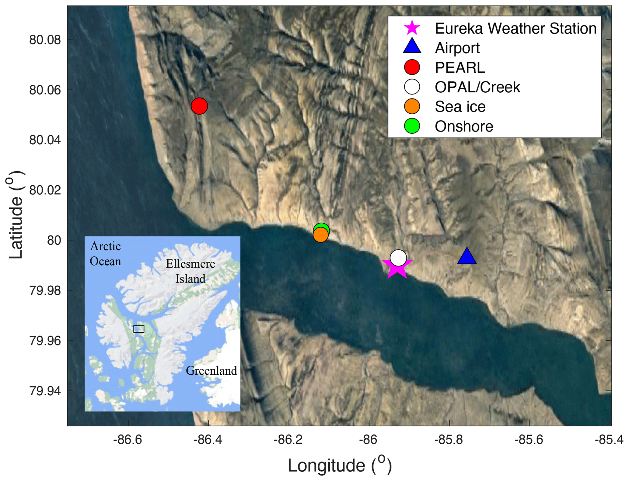
Figure 1 Local map with location of snow sampling sites marked by circles. The Eureka Weather Station (EWS) is marked by a star, and the Eureka airport is marked by a triangle. The small inset box shows the location of the main map of Ellesmere Island, Canada. Image copyright: © Google Earth/Google Maps.

Different methods have been used to derive the flux of deposited ions to snow (Cadle, 1991; Beine et al., 2003; Macdonald et al., 2017). For instance, Björkman et al. (2013) applied three different methods to derive nitrate dry deposition flux at Svalbard: tray sampling, glacial sampling, and modelling. Macdonald et al. (2017) derived major ion (including nitrate) deposition fluxes at Alert, Nunavut, from freshly fallen snow samples collected on average every 4 d. However, they could not derive bromide deposition flux, likely due to the efficient post-depositional loss of bromide given the sampling interval of 1 to 19 d. In this study we apply a methodology similar to, but slightly different from, that used by Macdonald et al. (2017). We deliberately increase temporal sampling resolution to ∼ 24 h and collect snow samples directly from the snowpack surface using a vertical resolution of 2–3 mm. This vertical resolution enables us to collect fresh falling snow from trace precipitation (an amount of precipitation greater than zero but too small to be measured by standard methods). Because of mixing of surface snow particles due to wind, samples collected in the skin layer are not solely from snow recently fallen in the past 24 h (with exceptions in very calm conditions); rather, they represent a mixture of various snow particles. Thus, ions measured in the surface layer are not only due to deposition in the past 24 h, but also to deposition in previous days. Therefore, by looking into the average change of ions within a timescale of 24 h, we can derive a mean net deposition flux of ions such as nitrate and bromide. To that end, we collected the top 1.5 cm of snow in three sub-layers: 0–0.2, 0.2–0.5, and 0.5–1.5 cm at several sampling sites (including onshore and offshore sites as well as on the top of a hill) in the high Arctic at Eureka (80° N, 86° W), Nunavut, Canada (Fig. 1), daily during early spring in 2018 and 2019. The aim of this study is to derive a net deposition flux of bromide and nitrate to surface snow and then to infer the role that snowpack plays as a direct source of reactive bromine and nitrogen. Methods and datasets are described in Sect. 2. The results are reported in Sect. 3. Discussions and atmospheric implications of this study are in Sect. 4, with conclusions given in Sect. 5.

2 Methods and datasets

2.1 Sampling site and local meteorology

Eureka is one of the coldest and driest places in the Canadian Arctic, with an average air temperature of −37 °C and precipitation of ∼ 2 mm in March. Surface inversions are frequently observed in winter–spring (∼ 84 % of the time), and boundary layer height is in the range of 400–800 m (Bradley et al., 1992). Due to the local geography and cold weather, sea ice near the Eureka Weather Station (EWS) is thick (e.g. > 1.5 m in early spring) and stable. Satellite-based sea ice data show that there are no clearly identifiable leads or open waters within 600–800 km to the north and west of Eureka in early spring (Bognar et al., 2020). Therefore, the impact of local open leads is negligible. In addition, modelling work shows that this area is only weakly influenced by open-ocean sea spray (Rhodes et al., 2017), thus open-ocean sourced bromine influence is of secondary importance (Yang et al., 2020). Under calm weather conditions, the atmospheric boundary layer at Eureka is generally shallow and stratified. Thus, the measurements made at the Polar Environment Atmospheric Research Laboratory (PEARL) Ridge Laboratory, located on the top of a hill (610 $\mathrm{m}\mathrm{a}.\mathrm{s}.\mathrm{l}.$) (Fig. 1), are mainly representative of the free tropospheric influence; however, under unstable condition such as cyclones, the PEARL Ridge Lab is within the extended boundary layer. In early spring, the UV index changes dramatically from very low levels at the end of February to higher levels at the end of March (Fig. S1 in the Supplement), mainly due to the rapid increase in daily solar elevation angles after polar sunrise on 21 February.

Sea water starts to freeze in late September at Eureka, with snow accumulating in the following months (before December). Therefore, snowpack depth does not change much after December, which is consistent with the results of an Arctic snow depth survey by Warren et al. (1999). On sea ice, snowpack depth near EWS is 10–30 cm, while snow depth inland varies from only a few centimetres at convex locations to more than half a metre at concave locations. The type of sea ice in the Slidre Fjord is mainly first-year ice. However, a large iceberg has been grounded in the fjord since summer 2018, which has significantly affected 2019 snow salinity and ionic concentrations on sea ice (see Sect. 3).

2.2 Snow sampling

As can be seen from Fig. 1, several sampling sites were located between EWS and the PEARL Ridge Lab. The two major sampling sites at sea level are ∼ 5 km to the west of EWS: one on sea ice (named “Sea ice,” ∼ 100 m offshore) and one onshore (named “Onshore,” ∼ 50 m inland). There are two additional inland sites (also close to sea level) just behind EWS: the PEARL “0PAL” (Zero Altitude PEARL Auxiliary Laboratory) site and the “Creek” site, which are close together and ∼ 1000 m from the sea ice. The PEARL Ridge Lab (hereafter, referred to as PEARL) is another major sampling site, which is ∼ 15 km to the west of EWS on top of a hill. In addition, a few snow samples were collected from the Eureka airport (∼ 70 $\mathrm{m}\mathrm{a}.\mathrm{s}.\mathrm{l}.$, ∼ 3 km to the east of EWS) and on the sea ice in front of EWS; however, these samples were not for ionic analysis due to local contamination concerns.

There are two types of surface snow observed at Eureka. One consists of fluffy mobile snow particles, loosely connected and white in colour. They mainly cover the top 0.5 cm of snow and are a mixture of recent falling snow, drifting snow, and deposited ice crystals. On slightly raised surfaces that face the predominant winds, there is a wind-crust layer that is light brown in colour and hard to break, representing aged snow. In 2018, these two types of surface snow were deliberately collected for salinity analysis. All samples were collected using their sampling tubes to scratch them from the surface, roughly at a depth of 0.3–0.5 cm.

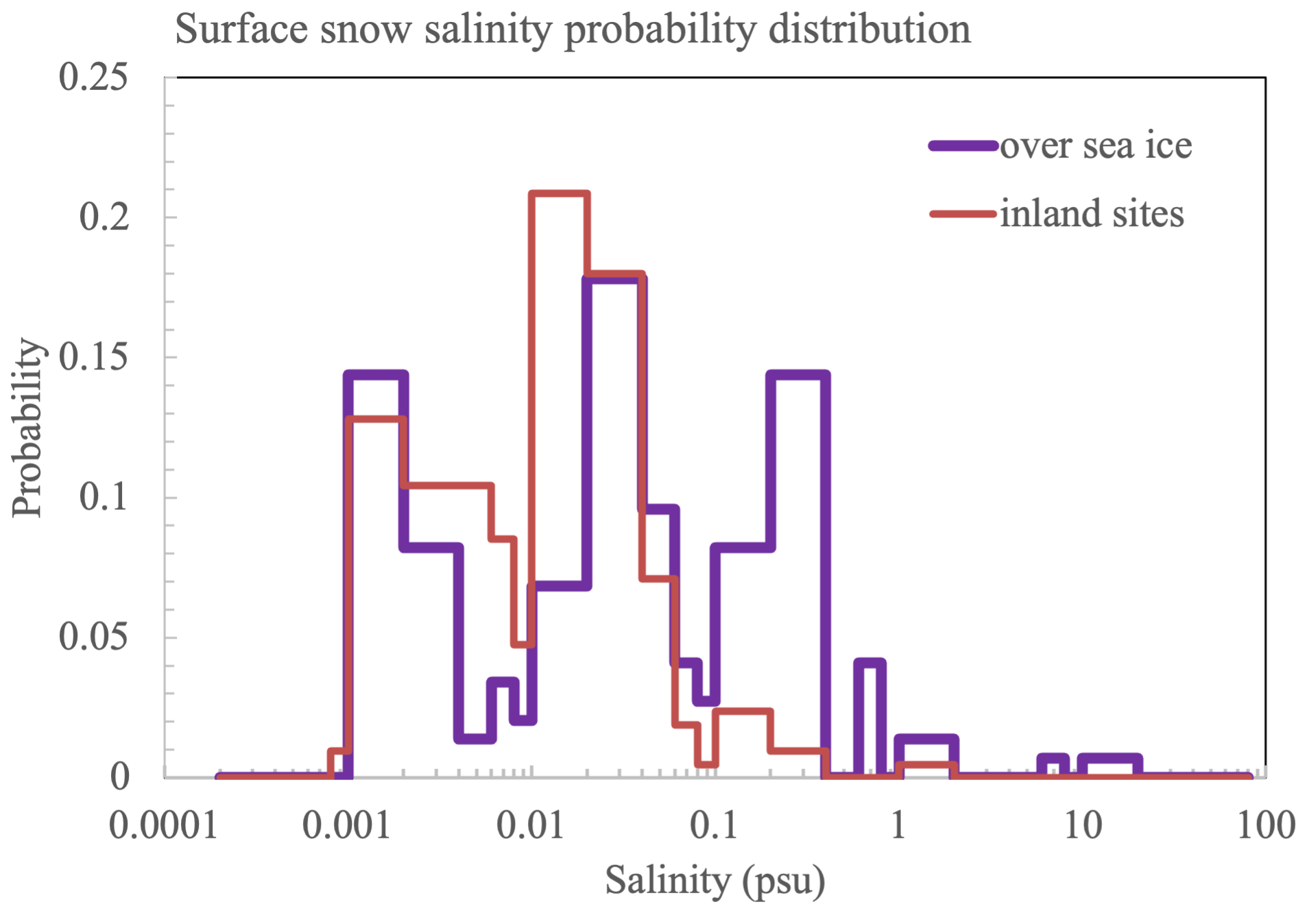
Figure 2 Eureka snow salinity probability distribution. The data include 2018 and 2019 snow sample measurements. The distribution over sea ice includes 146 snow samples, and the distribution at inland sites includes 211 snow samples (see Table 1).

A small patch of snow (about 1 m by 2 m) was identified at each major sampling site (Sea ice, Onshore, and PEARL) for daily snow sampling. In 2019, surface snow was collected using a small shovel with a funnel. Since 4 March, daily snow samples have been collected from three sub-layers (0–0.2, 0.2–0.5, and 0.5–1.5 cm). To investigate local geographic variation, a few snow samples were randomly collected across a distance of 1–2 m at each sampling site (from two snow layers: 0–0.5 and 0.5–1.5 cm between 26 February and 3 March). On 4 and 5 March, validation samples were collected during a precipitation event from three snow layers (0–0.2, 0.2–0.5, and 0.5–1.5 cm) at the 0PAL, Onshore, and Sea ice sites.

In addition to surface snow, airborne snow samples were collected on a daily basis using a mounted tray outside. For example, one tray was mounted outside the 0PAL building (∼ 1 m above the ground), and another one was mounted on the roof of the PEARL (∼ 1.5 m above the roof and ∼ 11 m above the ground). In windy conditions, most of the samples collected by trays consist of blowing snow particles. In calm conditions, trace samples from deposited ice crystals, and growing hoar frost at the edge of the tray can be collected. During precipitation events, freshly falling snow can be sampled. The trays were swept clean daily after snow sampling using a clean brush.

For logistical reasons, the time of day for surface snow sampling could not be fixed. Samples were normally collected either in the morning (09:30–11:00 local time) or in the afternoon (14:30–17:00 LT). This enables the samples to be used to investigate the photochemistry effect. Since 15 March 2019, the majority of samples from Sea ice and Onshore have been collected in the afternoon.

Column snow samples were collected (at a vertical resolution of 1–3 cm) from a few sampling sites at irregular intervals but mainly during 4–12 March in both 2018 and 2019. Ionic column results are reported based on seven 2019 columns (three at Sea ice and four at Onshore) and two 2018 columns (one at Sea ice and one at Onshore). Snow density was measured in 2018 at a vertical resolution of 3 cm using a snow cutter and a hanging scale. The snow density result is shown in Fig. S2.

2.3 Salinity measurements and ionic analysis

All snow samples collected were transferred to 50 mL polypropylene tubes with screw caps (Corning CentriStar), which prior to field deployment had been rinsed with ultra-high-purity (UHP) water and dried in a class 100 clean laboratory in Cambridge, UK. All tubes with samples were put in a dark bag for temporary storage before moving into ice core boxes for storage and transportation. One set of snow samples were melted in the 0PAL laboratory to measure aqueous conductivity using a conductivity meter (SensIon 5, Hach) with a measurement range of 0–200 mS cm⁻¹ and a maximum resolution of 0.1 µS cm⁻¹ at low conductivities (0–199.9 µS cm⁻¹). Conductivity values were converted into psu, approximately equivalent to the weight of dissolved inorganic matter in g kg⁻¹ of seawater. Accuracy as stated by the manufacturer is ± 0.001 psu at low salinities (< 1 psu). Results are shown in Fig. 2.

The 2018 snow samples were shipped frozen back to Cambridge, UK, shortly after the campaign, and the 2019 samples were shipped frozen directly to the Canadian Ice Core Lab (CICL) at the University of Alberta. All samples were only melted prior to the ion chromatography (IC) analysis, apart from a small portion of the samples that had been melted for salinity measurements. The 2018 samples were analysed in October 2018, and the 2019 samples were analysed in December 2019. Elevated salinity samples were diluted with UHP water, typically by a factor of 10 or 100 based on the estimated salinity. Due to the presence of fine particulates in the snow samples, all 2019 samples were filtered using Millex-GP Express PES Membrane, Sterile, 33 mm, 0.22 µm filters (Merck Millipore Ltd., Cork, Ireland). The 2018 snow samples were analysed using Thermo Scientific Dionex ICS-4000 ion chromatography systems, with ions of Na⁺, Ca²⁺, Mg²⁺, K⁺, ${\mathrm{NH}}_{\mathrm{4}}^{+}$, Cl⁻, Br⁻, ${\mathrm{SO}}_{\mathrm{4}}^{=}$, ${\mathrm{NO}}_{\mathrm{3}}^{-}$, F⁻, acetate, formate, oxalate, and methanesulfonic acid (MSA) measured. The 2019 samples for IC analysis were run on a Dionex ICS-5000+ with ions of Na⁺, Ca²⁺, Mg²⁺, K⁺, Cl⁻, Br⁻, ${\mathrm{SO}}_{\mathrm{4}}^{=}$, ${\mathrm{NO}}_{\mathrm{3}}^{-}$, and MSA measured. Anion analysis was performed using an IonPac AS18-Fast-4 µm column, and cation analysis was performed using an IonPac CS12A column. The eluents for ion chromatography were generated with a Dionex hydroxide eluent generation cartridge (EGC) for anion analyses and a Dionex methanesulfonic acid EGC for cation analyses.

Multiple samples (in 2019) were analysed to assess precision. The relative standard deviations of duplicate analyses, limits of detection (LOD = 3 times standard deviation of filter blank average peak area), and limits of quantification (LOQ = 10 times standard deviation of filter blank average peak area) for all sequences (∼ 40 samples analysed per sequence) are reported in Table S1 in the Supplement. The LOD of Br⁻ is 0.200 µM with a relative standard deviation of 0.023 µM, and the LOD of ${\mathrm{NO}}_{\mathrm{3}}^{-}$ is 0.484 µM with a relative standard of deviation of 0.037 µM. The mean statistical results for the ionic analysis of the 2018 and 2019 samples are given in Tables S2 and S3, respectively. Mean values excluded outliers, defined as values more than 1.5 interquartile ranges above the upper quartile or below the lower quartile. Column means were calculated using values exclusively within the depth range ≥ 1.5 and ≤ 20 cm. Interpolation for vertical profile data consisted of 2 cm bin averages from 1.5 cm depth to the bottom of the snowpack.

2.4 MAX-DOAS measurements and BrO retrieval

Multi-axis Differential Optical Absorption Spectroscopy (MAX-DOAS) measurements of BrO partial columns were performed at the PEARL Ridge Lab. Spectra were recorded in the ultraviolet (UV) using a grating spectrometer (spectral resolution 0.45 nm) with a cooled (200 K) charge-coupled device (CCD) detector at 0.4–0.5 nm resolution. Elevation angles of 30, 15, 10, 5, 2, 1, and −1° were used in the elevation scans, and measurements were only taken with solar elevation above 4°. Differential slant column densities (dSCDs) of BrO and the oxygen dimer (O₄) were retrieved using the DOAS technique with the settings described in Zhao et al. (2016) and Bognar et al. (2020). Reference spectra for the DOAS analysis were temporally interpolated from zenith measurements taken before and after each elevation scan. dSCDs were converted to profiles using a two-step optimal estimation method (Frieß et al., 2011). First, aerosol extinction profiles were retrieved from O₄ dSCDs, and then the extinction profiles were used as a forward model parameter in the BrO vertical profile retrieval. The retrievals were performed for 0–4 km  altitude on a grid with 0.2 km resolution. Due to the elevation of the measurement site, the instrument often measures BrO in the free troposphere, except during strong wind episodes and storms that generate a deep boundary layer (Bognar et al., 2020).

2.5 Complementary datasets

There are two sets of local meteorology data used in this work: one from EWS (the archived data are available at Historical Data – Climate – Environment and Climate Change Canada, ECCC, https://weather.gc.ca, last access: 14 May 2024) and one from the PEARL Ridge Lab. In addition to the continuous datasets such as pressure, temperature, and wind speeds, archived hourly data were used to derive daily weather conditions such as blowing snow events, fog, ice crystals, and trace precipitation. In addition, ECMWF 6-hourly interim (ERA-interim) meteorological data were used to explore large-scale weather conditions. Surface ozone measurements were made by a TEI 49i ozone analyser deployed at 0PAL (Bognar et al., 2020). Hourly mean surface ozone data are available since the instrument was installed in late 2016. The UV index measured during the campaign period in 2018 and 2019 is shown in Fig. S1 (and data from the ECCC Brewer spectrophotometer available within Fioletov et al., 2005). In addition, NOAA back-trajectory output from the Hybrid Single-Particle Lagrangian Integrated Trajectory (HYSPLIT) model (Stein et al., 2015; Rolph et al., 2017) is used for diagnosing the air-mass history of selected events.

3 Results

3.1 Snow salinities

Figure 2 shows snow salinity distributions over sea ice (purple) and inland (orange) from all measurements, except for the tray samples. Inland snow has a dual peak distribution with the first and second peaks appearing at 0.001–0.002 and 0.01–0.04 psu, respectively. On sea ice, snow has a triple peak distribution, with the first and second peaks overlapping with the inland peaks, indicating similar origins. The third peak at 0.2–0.4 psu clearly reflects sea water influence.

Table 1 Mean and median snow salinities (psu) in various snow samples: tray, at inland and sea ice sites. Surface snow (< 0.5 cm) salinities are in two snow types: fluffy soft snow and aged hard snow.

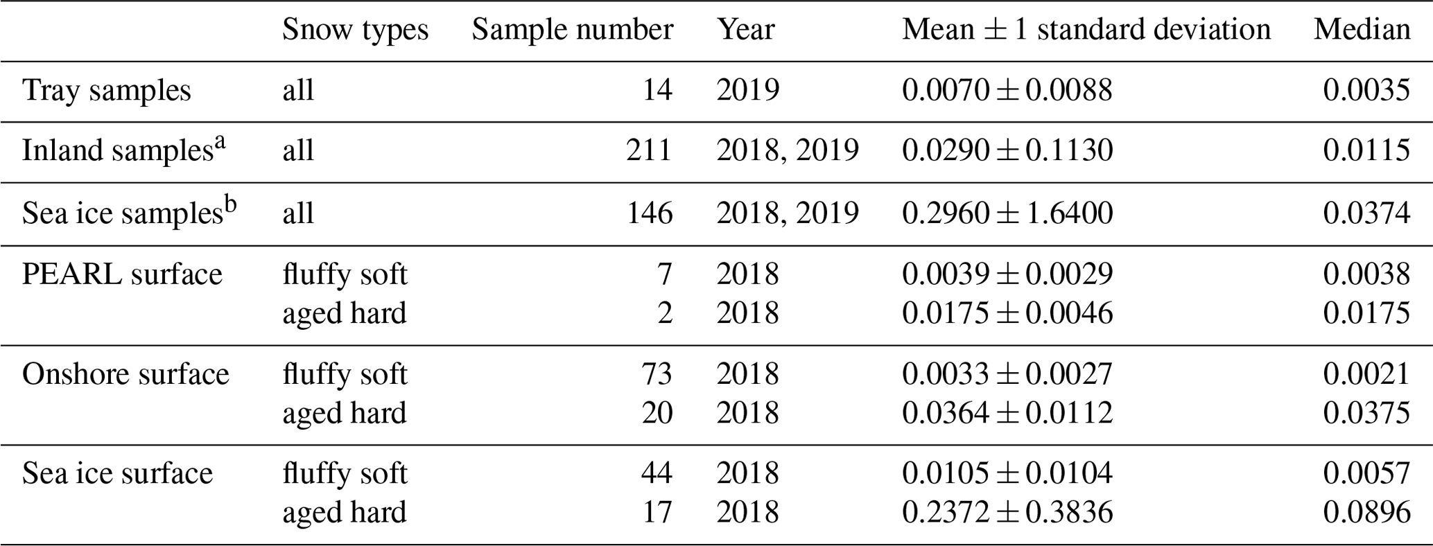
^a Inland data contain all salinity measurements for snow samples in the surface layers and columns collected at the Onshore, 0PAL/Creek, PEARL, and airport sites. ^b Sea ice data contain all salinity measurements for samples in the surface layers and columns collected over sea ice (see Sect. 2.2).

Table 1 shows mean and median snow salinities (psu) in tray samples at inland and sea ice sites, as well as in two snow types: soft fluffy snow and aged hard snow. Tray samples have the lowest mean value of 0.0070 ± 0.0088 psu (N=14), which is lower than the inland mean (0.0290 ± 0.113 psu, N=211) and the Sea ice mean (0.296 ± 1.640 psu, N=146) by ∼ 4 times and ∼ 40 times, respectively. The lowest tray sample salinity of 0.00178 psu corresponded to a falling snow event on 6 March 2019 in calm weather conditions and is close to the first-peak salinity obtained in the surface layer snow indicating that this first peak of surface snow salinity (0.001–0.002 psu) is likely due to the precipitation dilution effect (due to less salt in falling snow). The tray samples median of 0.0035 psu is roughly $\mathrm{1}/\mathrm{3}$ and $\mathrm{1}/\mathrm{10}$ of the inland and sea ice sample median values (0.0115 and 0.0375 psu, respectively) but close to their second salinity peak, which is in line with the fact that the majority of tray samples are wind-blown particles.

The salinity difference between the two types of surface snow is significant. For example, at PEARL, the mean salinity of the soft fluffy snow is 0.0039 ± 0.0029 psu (N=7), which is ∼ 4 times less than that of the hard aged snow (0.0175 ± 0.0046 psu, N=2). At the Onshore site, the difference is ∼ 11-fold (0.00327 ± 0.00273 psu, N=73, vs. 0.0364 ± 0.0112 psu, N=20). At the sea ice site, the difference increases to ∼ 23-fold (0.0105 ± 0.0104 psu, N=44, vs. 0.2372 ± 0.3836 psu, N=17). Comparing these values with the snow salinity distributions in Fig. 2, the soft fluffy snow salinity is seen to overlap well with the first peak, and the aged snow salinity overlaps well with the second peak. This indicates that fresh falling snow and the subsequent salt accumulation effect (due to water vapour loss by sublimation) are responsible for the first and the second salinity peak, respectively. The third salinity peak (0.2–0.4 psu) on sea ice is likely due to the sea water effect (due to upward migration of brine), which is also observed in Weddell Sea surface snow (Fig. 16 in Frey et al., 2020). In addition, the second snow salinity peak on sea ice (0.02–0.04 psu) is consistent with Weddell Sea snow salinity on multi-year sea ice, which indicates that the salts on multi-year ice surface layers could be a result of the accumulation effect for deposited salts following the sublimation of water vapour rather than a direct sea water impact from the bottom (via the so-called wicking migration effect). However, the Weddell Sea snow salinity does not resolve the first salinity peak at 0.001–0.002 psu observed in Eureka, which could be due to the coarse vertical sampling resolution (2–3 cm) applied in their sampling.

Figure 3 shows surface snow salinity vertical profiles from the first layer (0–0.2 cm) to the third layer (0.5–1.5 cm), and Fig. S3 shows column salinity profiles. Note that tray sample salinity is shown in the upper panel of Fig. 3. Salinity in the third layer is ∼ 8 and ∼ 15 times that of the first layer at the Onshore site and the Sea ice site, respectively. The larger vertical gradient seen on sea ice is likely due to sea water influence from below. At PEARL, the vertical trend is not clear, perhaps due to the very thin, soft fluffy layer (only a few millimetres) and the thick crust layer observed at the top of the hill where winds are stronger. Generally, tray sample salinity at the 0PAL site is on average larger than that at the PEARL site; a similar result is also reflected in major ions such as [Cl⁻] and $\left[{\mathrm{NO}}_{\mathrm{3}}^{-}\right]$ (Figs. 4 and S4). The relatively low salinity at the PEARL site is likely attributed to the higher geographic altitude (∼ 600 m) and the higher height of the mounted tray above the ground (e.g. ∼ 11 m at PEARL versus ∼ 1 m at 0PAL).

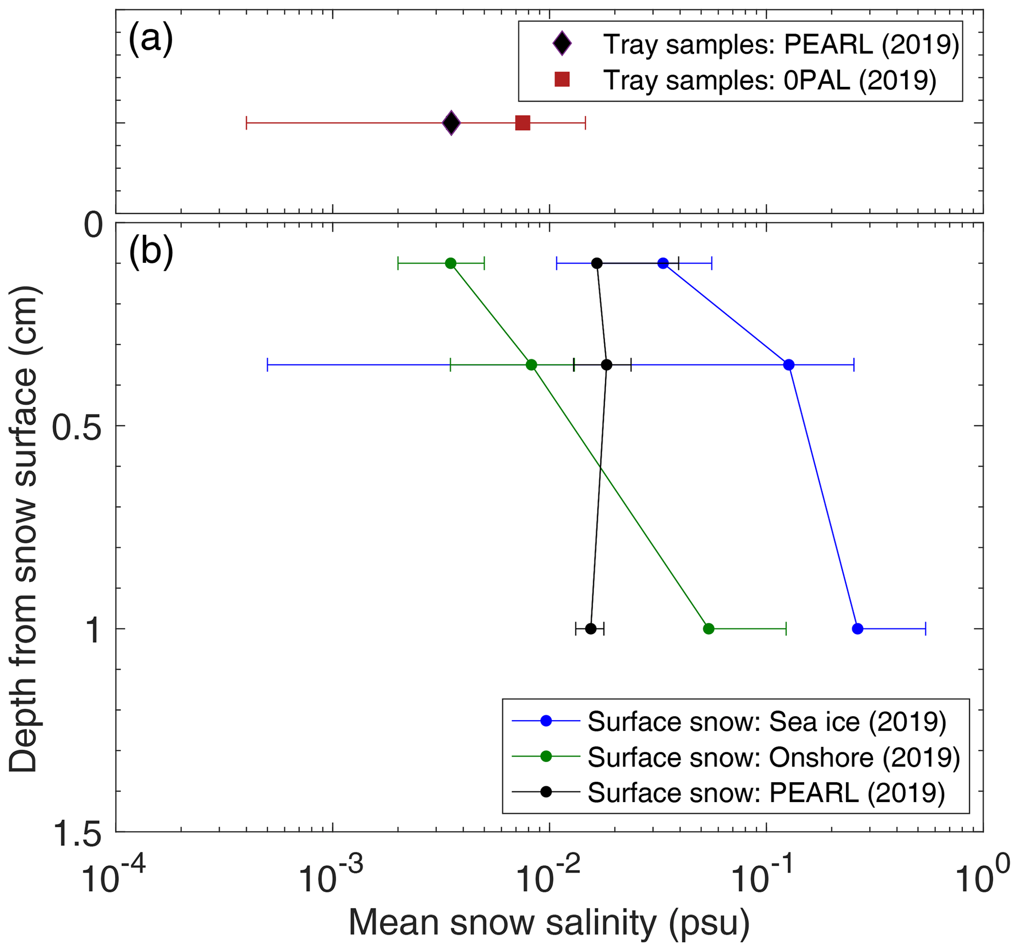
Figure 3 Mean snow salinity from the top 1.5 cm in three sub-layers: 0–0.2, 0.2–0.5, and 0.5–1.5 cm at the Sea ice, Onshore, and PEARL sites (b) and tray sample salinity at the 0PAL and PEARL sites (a). The horizontal error bar represents 1 standard deviation. Note that tray samples at 0PAL were from a mounted tray outside the 0PAL building, approximately 1 m above the ground. Tray samples at PEARL were from a mounted tray (∼ 1.5 m) on the roof of the PEARL Ridge Laboratory (∼ 11 m above the ground).

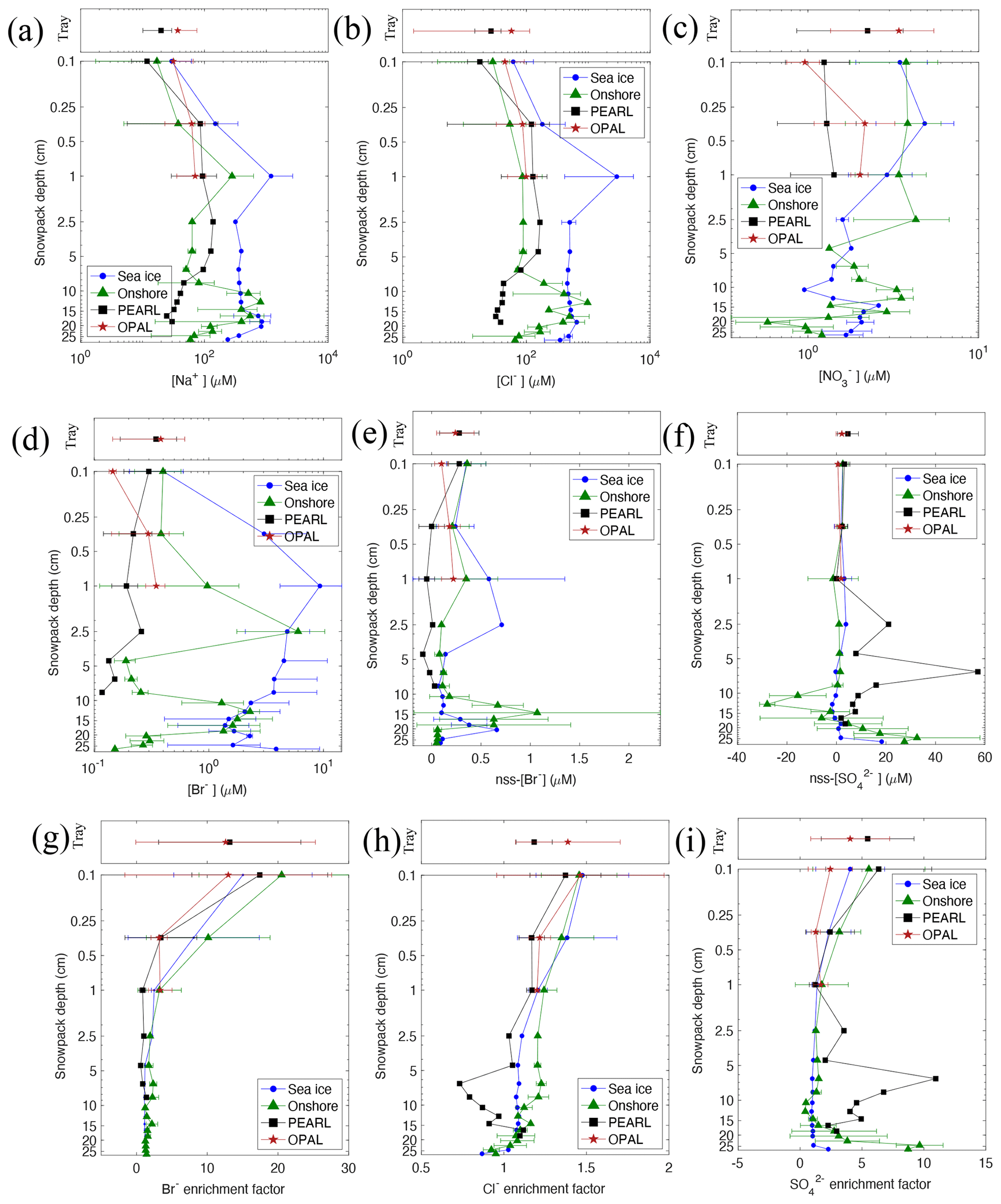
Figure 4 Vertical profiles of 2019 snow ions [Na⁺] (a), [Cl⁻] (b), $\left[{\mathrm{NO}}_{\mathrm{3}}^{-}\right]$ (c), [Br⁻] (d), non-sea-salt (nss)[Br⁻] (e), and $\mathrm{nss}\left[{\mathrm{SO}}_{\mathrm{4}}^{\mathrm{2}-}\right]$ (f) and enrichment factor of [Br⁻] (g), [Cl⁻] (h), and $\left[{\mathrm{SO}}_{\mathrm{4}}^{\mathrm{2}-}\right]$ (1) (see Sect. 3.2 for details).

The column salinity profiles in Fig. S3 are predominantly 2018 data. Snow salinities at all inland sites do not vary much with distance from the surface. PEARL has the lowest column mean salinity (0.0023 ± 0.0019 psu). Onshore has > 10 times the salinity (0.036 ± 0.034 psu). The highest column mean snow salinity was observed on sea ice in 2018, with a mean value (top 20 cm) of 1.673 ± 2.09 psu; the maximum salinity of 18.73 psu was measured at the sea ice interface sample. It is interesting to note that the 2019 column mean on sea ice (top 20 cm) is very low (0.085 ± 0.026 psu), about 20 times lower than the 2018 value, which is likely due to the dilution effect from the large iceberg grounded near Eureka.

The snow depth at the 2018 Sea ice sampling site is in the range of 24–28 cm, and a similar snow depth range (25–29 cm) was measured at the 2019 Sea ice site; this is partly because we deliberately chose a similar snow depth for sampling. In addition, the measured precipitation amount between October 2017 and March 2018 is 20 mm, and the amount between October 2018 and March 2019 is 19.4 mm, implying a similar snow depth on sea ice. Therefore, the significant difference in column snow salinity between these two years cannot be due to snowpack depth difference; rather the difference could be due to the saline supply at the sea ice interface. For example, the 2019 bottom snow (1–3 cm above the sea ice interface) salinity is lower than the 2018 bottom snow salinity by more than an order of magnitude (Fig. S3), indicating a possible dilution effect in 2019 from the iceberg grounded near EWS.

3.2 Ion concentrations

Figure 4 shows vertical profiles of 2019 snow ions [Na⁺], [Cl⁻], $\left[{\mathrm{NO}}_{\mathrm{3}}^{-}\right]$, [Br⁻], non-sea-salt bromide (noted as nss[Br⁻] = [Br⁻]_obs − 0.0018 × [Na⁺]_obs), non-sea-salt $\left[{\mathrm{SO}}_{\mathrm{4}}^{\mathrm{2}-}\right]$ ($\mathrm{nss}\left[{\mathrm{SO}}_{\mathrm{4}}^{\mathrm{2}-}\right]$ = $[{\mathrm{SO}}_{\mathrm{4}}^{\mathrm{2}-}{]}_{\mathrm{obs}}$ − 0.601 × [Na⁺]_obs), and enrichment factors of Br⁻, Cl⁻, and ${\mathrm{SO}}_{\mathrm{4}}^{\mathrm{2}-}$. Non-sea-salt values are calculated with the aim of removing salt effects on the concentration of bromine and sulfate, which assists data interpretation particularly in comparisons between offshore and onshore sites as well as from different snow depths. The enrichment factor is calculated following the equation of EF_x = $\left(\left[X\right]/[\mathrm{Na}{]}_{\mathrm{obs}}\right)/\left(\left[X\right]/[\mathrm{Na}{]}_{\mathrm{seawater}}\right)$, where $\left[X\right]/[\mathrm{Na}{]}_{\mathrm{obs}}$ represents the ratio of ion X to sodium in a sample, and $\left[X\right]/[\mathrm{Na}{]}_{\mathrm{seawater}}$ is the ratio in standard sea water (Wilson, 1975). If EF_Y > 1.0, ion X is enriched, and if < 1.0 it is depleted. To highlight the surface snow results, a lognormal y axis is applied. Tray sample results are plotted in the top panel of each plot. Figure S4 shows the remaining profiles, including [Ca²⁺], [Mg²⁺], [K⁺], and $\left[{\mathrm{SO}}_{\mathrm{4}}^{\mathrm{2}-}\right]$ and enrichment of [Ca²⁺], [Mg⁺], and [K⁺].

As can be seen from Fig. 4a and data in Table S3, the tray sample mean [Na⁺] (19.86 ± 9.78 µM) at PEARL is 1.7 times that of the first-layer mean (11.80 ± 5.20 µM), and at 0PAL, and the tray sample mean [Na⁺] (36.99 ± 23.25 µM) is 1.2 times that of the first-layer mean (31.33 ± 34.37 µM). For [Cl⁻] (Fig. 4b), the factor is 1.5 and 1.3 times at PEARL and 0PAL, respectively. The enhancement of tray sample salts is likely due to the accumulation effect following water loss via sublimation processes. However, this accumulation effect cannot explain the even larger enhancement in $\left[{\mathrm{NO}}_{\mathrm{3}}^{-}\right]$ and nss[Br⁻] seen in Fig. 4c and e, respectively. For instance, at 0PAL the tray sample mean $\left[{\mathrm{NO}}_{\mathrm{3}}^{-}\right]$ (3.41 ± 2.05 µM) is 3.6 times the first-layer mean (0.96 ± 0.21 µM), and at PEARL the tray sample $\left[{\mathrm{NO}}_{\mathrm{3}}^{-}\right]$ (2.23 ± 1.37 µM) is 1.8 times the first-layer mean (1.24 ± 0.50 µM). Eureka snow $\left[{\mathrm{NO}}_{\mathrm{3}}^{-}\right]$ is close to fresh snow nitrate of 2.5 µM at Alert in winter (Mcdonald et al., 2017) but smaller than snow nitrate of ∼ 7 µM in Utqiaġvik (formerly Barrow), Alaska (Krnavek et al., 2012).

For nss[Br⁻], at 0PAL, the tray sample mean (0.24 ± 0.19 µM) is 2.4 times the first-layer mean (0.10 ± 0.07 µM). This indicates that airborne snow particles may uptake more gaseous nitric acid and soluble bromine species from the air than snow on the ground. The deposition rate of chemical compounds to the ground is controlled by a series of transport steps – aerodynamic, sub-layer of the boundary, and surface resistance (Wu et al., 1992).

Similar to snow salinity profiles (Fig. 3), 2019 surface snow [Na⁺] (and [Cl⁻]) increases significantly from the first layer to the third layer, e.g. by about 20-fold at Onshore, 30-fold at Sea ice, and 8-fold at PEARL (Fig. 4a and b). The lowest sodium concentrations in the first layer are likely due to the precipitation dilution effect (due to less salt in falling snow particles). [Br⁻] (Fig. 4d) and [${\mathrm{SO}}_{\mathrm{4}}^{=}$] (Fig. S4d) show a similar vertical gradient; however, nss[Br⁻] (Fig. 4e) and nss[${\mathrm{SO}}_{\mathrm{4}}^{=}$] (Fig. 4f) do not show such an increasing trend, indicating the surface layer enhancement of the salts is largely due to the accumulation effect. Moreover, the first-layer nss[Br⁻] is generally higher than the second layer (0PAL is an exception), indicating the deposited bromide is from the air. A similar result is also seen in the bromine enhancement factor (Fig. 4g). Regarding the 0PAL exception, this is mainly due to the two days when samples were collected during and shortly after the precipitation event (on 4 and 5 March 2019).

The first-layer [Br⁻] (Fig. 4d) at Sea ice (0.40 ± 0.20 µM, N=40) and Onshore (0.40 ± 0.17 µM, (N=38) is almost the same; however, in the second and third layers, [Br⁻] at Sea ice (3.03 ± 4.14 µM, N=51) is significantly higher than that at Onshore (0.38 ± 0.22 µM, N=58) by more than an order of magnitude. When the sea water contribution is removed, the nss[Br⁻] concentrations (Fig. 4e) are not significantly different from each other (0.24 ± 0.19 µM (N=32) vs 0.21 ± 0.17 µM, N=50), strongly indicating similar atmospheric influences at the two sites.

The column mean nss[Br⁻] value at Sea ice is 0.22 ± 0.18 µM (N=17) and at Onshore is 0.30 ± 0.31 µM (N=89). Both values are positive, indicating a net sink of atmospheric bromine prior to the measurements. However, at PEARL the positive nss[Br⁻] was only observed in the tray samples (0.28 ± 0.20 µM, N=21) and the first snow layer (0.28 ± 0.12 µM, N=31). The column mean nss[Br⁻] at PEARL is −0.05 ± 0.08 µM (N=34) (Table S3), indicating snowpack at the top of the hill is bromide depleted. Due to the lack of temporal variation information, the timing of the bromine depletion cannot be determined (e.g. before or after the precipitation), nor whether it occurred soon after sunrise on 21 February. The 2018 snow samples at PEARL do not show clear bromine depletion (Fig. S5d), as the column mean nss[Br⁻] is slightly positive (0.01 ± 0.01 µM, N=8) (Table S2). Snow bromide enrichments were reported at other Arctic sea level locations, e.g. in the vicinity of Utqiaġvik (formerly Barrow), Alaska (Simpson et al., 2005), at other Canadian Arctic Archipelago sites (Xu et al., 2016), and on first-year sea ice (Peterson et al., 2016). However, at elevated sites in Svalbard (i.e. a few hundred metres above sea level), both bromide enrichment (Spolaor et al., 2013) and depletion (Jacobi et al., 2019) were measured.

Figure 4g–i show enrichment factors for Br⁻, Cl⁻ and ${\mathrm{SO}}_{\mathrm{4}}^{\mathrm{2}-}$ in 2019 snow samples. All these anions are significantly enriched in surface layers and in tray samples, indicating important airborne sources. In particular, the calculated ${\mathrm{EF}}_{{\mathrm{Br}}^{-}}$ values in the tray samples and the first and second layers are larger than 10. Due to the lack of simultaneous measurements of soluble inorganic bromine and filter aerosols, the dominant form of deposited bromide is unknown. Figure S4 shows that cations [Ca²⁺], [Mg⁺], and [K⁺] are also enriched, especially in the bottom part at inland sites. In particular, [Ca²⁺] enrichment factors at Onshore and PEARL sites are larger than 10, indicating strong terrestrial dust influence during the late autumn when the land is not completely covered by snow.

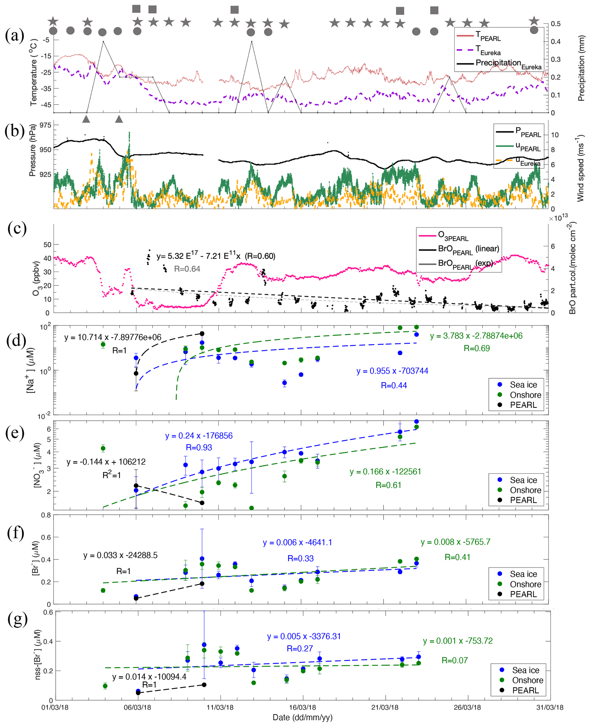
Figure 5 Time series of 2018 data. Air temperature at Eureka Weather Station (EWS) and PEARL and daily total precipitation (≥ 0.2 mm) are shown in (a). Local weather conditions are marked by symbols in (a) and (b): squares represent fog (> 2 h), stars represent ice crystals (> 2 h), circles represent trace precipitation (> 2 h), and triangles represent blowing snow (> 2 h). Atmospheric pressure at EWS and wind speeds at EWS and PEARL Ridge Laboratory are plotted in (b). One-hourly surface ozone at 0PAL and MAX-DOAS BrO (0–4 km) partial columns from the PEARL Ridge Laboratory are in (c). The exponential regression for BrO data is shown by a dashed grey line with regression function and correlation coefficient R value given in brackets; the linear regression curve is also added with R value shown only. Note that the BrO data time is in fraction of day and counted from 1 January 1970. Top 0.5 cm snow [Na⁺] (d), $\left[{\mathrm{NO}}_{\mathrm{3}}^{-}\right]$ (e), [Br⁻] (f), and nss[Br⁻] (g) and corresponding linear regression function against time and correlation coefficient R at each site are given. More statistical details of the linear regressions in each panel are given in Table S5.

Like snow salinity results, major snow ions on sea ice also have a large perturbation from 2018 to 2019. For example, the 2018 column mean snow sodium on sea ice (Tables S2 and S3) is 3–4 times that of the 2019 column mean, which is consistent with the relatively low snow salinity observed in 2019 due to the presence of a large iceberg grounded in the valley. In 2018, the column mean (1.5–20 cm) bromide on sea ice is 10.74 ± 8.52 µM (N=80) (Table S2), while in 2019 it is only 6.47 ± 5.36 µM (N=66) (Table S3). The lower 2019 snow bromide on sea ice is likely attributed to the freshwater dilution by the iceberg. However, they are both much smaller than mean 30.6 µM on thick first-year ice (FYI) and 92.5μM on thin FYI in Utqiaġvik (formerly Barrow), Alaska (Krnavek et al., 2012). Yet, surface snow bromide does not follow the column mean pattern; instead, the 2018 surface snow bromide is even lower than that of the 2019 values. For example, bromide in the top 0.5 cm snow layer in 2018 is 0.23 ± 0.10 µM (N=36), which is significantly lower than the 2019 value of 0.40 ± 0.20 µM (N=40) in the 0–0.2 cm layer and the value of 3.03 ± 4.14 µM (N=51) in the 0.2–0.5 cm layer. The lower 2018 surface snow bromide loading is likely related to the extremely low BrO partial columns measured in March at Eureka by MAX-DOAS (Bognar et al., 2020), during which unusually calm weather, low aerosol optical depth (AOD), and coarse-mode aerosol (likely SSA) concentrations were observed (see Sect. 3.3 and Fig. 5 below for more details). These results indicate that top layer snow bromide is largely controlled by atmospheric processes rather than by the underlying snowpack. This conclusion is also consistent with previous findings that bromide concentrations at low salinities are dominated by atmospheric exchange (Krnavek et al., 2012). Interestingly, surface layer nitrate concentrations between 2018 and 2019 are not significantly different. For example, the 2018 top 0.5 cm snow nitrate on sea ice is 3.13 ± 1.00 µM (N=33), comparable to the 2019 first-layer nitrate on sea ice of 3.46 ± 1.55 µM (N=37).

3.3 Geographic heterogeneity of snow bromide and nitrate

Using the samples collected between 26 February and 3 March 2019, local geographic differences (across distances of 1–2 m) of snow sodium, nitrate, and bromide were assessed at each sampling site (Table S4). For bromide, the smallest heterogeneity is found at inland sites, particularly at PEARL, with the largest heterogeneity at Sea ice. For example, top 0.5 cm snow [Br⁻] is 0.28 ± 0.14 µM (nss[Br⁻] = −0.05 ± 0.07 µM) at PEARL, compared to [Br⁻] of 0.30 ± 0.13 µM (nss[Br⁻] = 0.25 ± 0.13 µM) at Onshore and 0.67 ± 0.74 µM (nss[Br⁻] = 0.43 ± 0.48 µM) at Sea ice. Deeper-layer snow bromide heterogeneity is generally larger than the upper layer (with an exception at PEARL), which is likely due to the large uncertainty of accumulated bromide. The smallest standard deviation of nss[Br⁻] is at PEARL (0.075 µM), with the medium value of 0.21 µM at Onshore, and the largest 0.73 µM at Sea ice. Nitrate in the top 0.5 cm and the 0.5–1.5 cm layer are not significantly different, indicating they are independent of snow salts. The top 1.5 cm mean $\left[{\mathrm{NO}}_{\mathrm{3}}^{-}\right]$ at Sea ice is 3.62 ± 1.34 µM, at Onshore is 2.95 ± 0.86 µM, and at PEARL is 2.03 ± 0.43 µM. As with bromide, PEARL has the smallest mean value and uncertainty. Note that the source of uncertainty is not solely from geographic variation; other factors such as temporal variations (see Sect. 3.4) as well as the bias in depth estimation all contribute to the uncertainty.

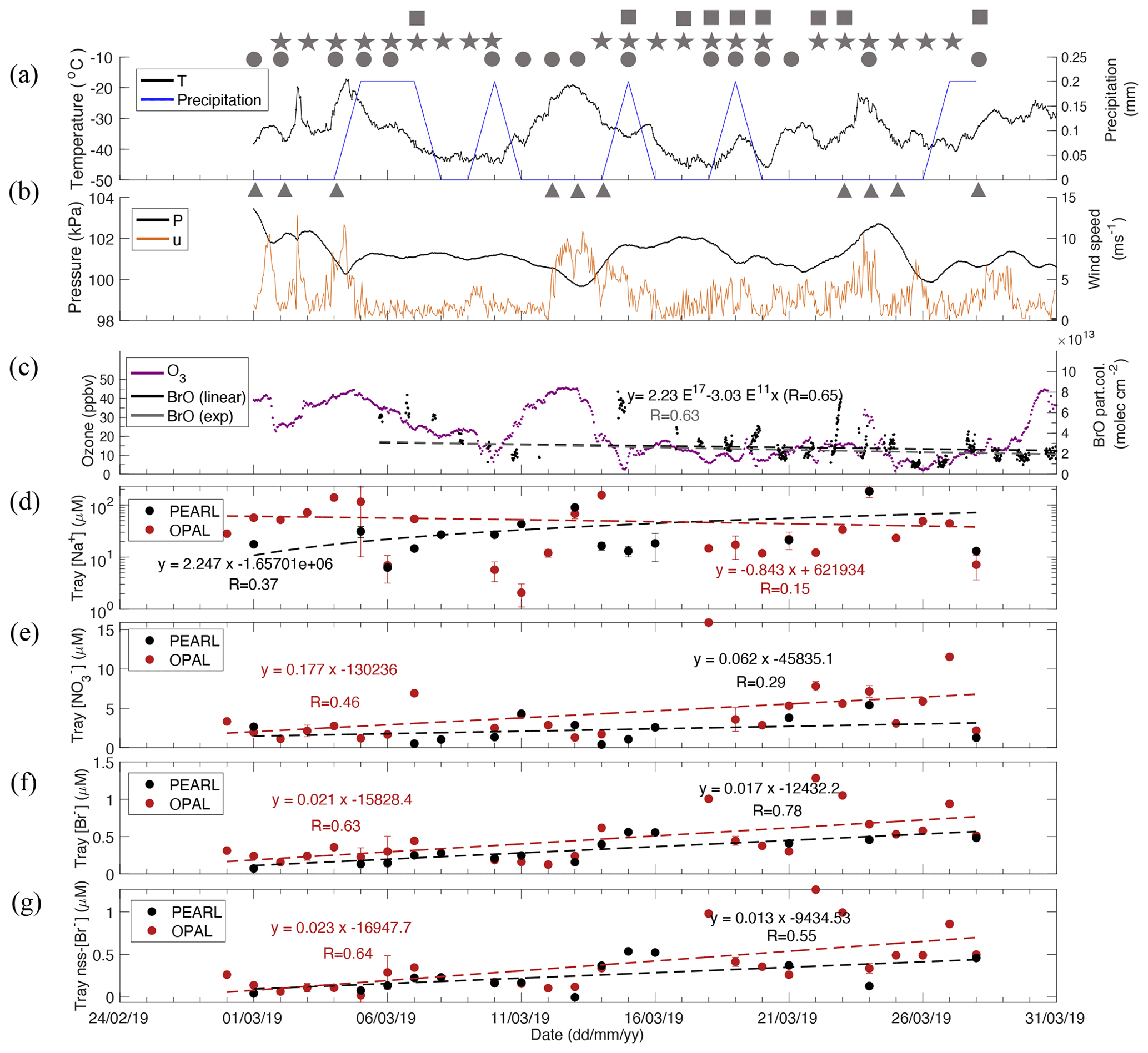
Figure 6 Same as Fig. 5 but for 2019 snow time series. Note that the meteorology data are only from the Eureka Weather Station, and the ionic data are tray samples [Na⁺] (d), $\left[{\mathrm{NO}}_{\mathrm{3}}^{-}\right]$ (e), [Br⁻] (f), and non-sea-salt (nss)[Br⁻] (g). Table S5 gives more statistical details of the linear regressions in each panel. Local weather conditions are marked by symbols in (a) and (b). Squares represent fog, stars represent ice crystals, circles represent trace precipitation, and triangles represent blowing snow.

On 4 and 5 March 2019, snow samples were collected during a precipitation event (Fig. 6a) from three sub-layers (0–0.2, 0.2–0.5, and 0.5–1.5 cm) at the 0PAL, Onshore, and Sea ice sites (also in Table S4). The 0.2 mm precipitation measured meant a ∼ 1 cm snowfall on the surface, which explains the low concentrations and low variability of [Br⁻] at Onshore. Moreover, the top 0.2 cm snow [Br⁻] (0.12 ± 0.00 µM) at Onshore is very close to that for 0PAL (∼ 5 km away) (0.14 ± 0.02 µM), indicating they are under the same atmospheric influence. However, at Sea ice the first-layer [Br⁻] (0.38 ± 0.04 µM) is ∼ 3 times that of the onshore value, highlighting the underlying sea ice effect. The sea ice effect is more significant in the second (0.2–0.5 cm) layer, where high [Br⁻] (5.73 ± 5.57 µM) was measured. However, the corresponding nss[Br⁻] (0.01 ± 0.04 µM) in the second layer at Sea ice is very low and close to the nss[Br⁻] (0.01 ± 0.00 µM) at 0PAL, also indicating the same atmospheric influence. For nitrate, the precipitation effect is less significant; the sea level mean $\left[{\mathrm{NO}}_{\mathrm{3}}^{-}\right]$ (3.28 ± 1.10 µM) is very close to the Sea ice mean obtained during 26 February–3 March. The sea level nitrate is also higher than the hilltop mean of 2.03 ± 0.43 µM, indicating a vertical gradient of atmospheric nitrogen oxide between the boundary layer and the free troposphere.

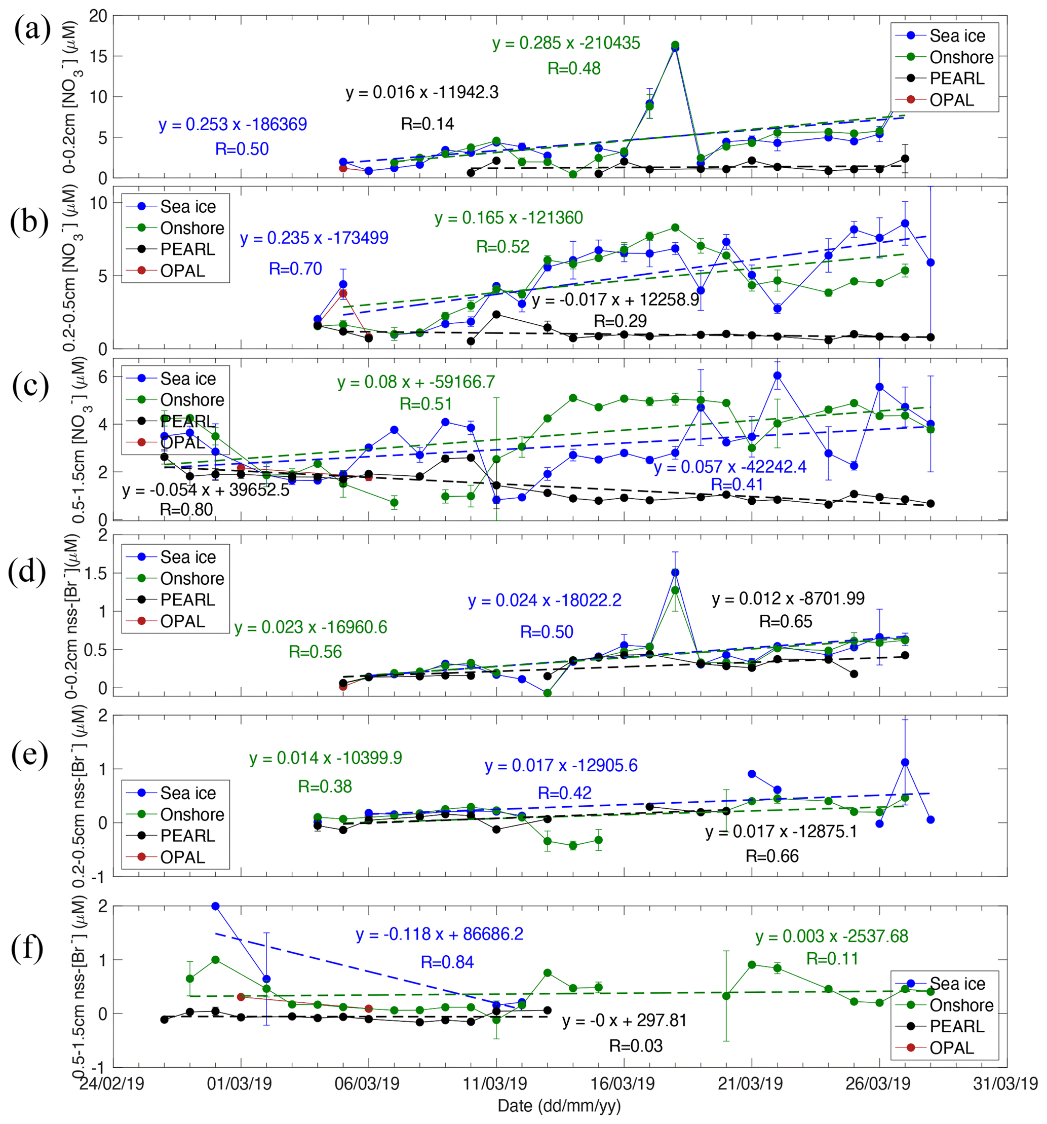
Figure 7 Time series of 2019 snow nitrate (a–c) and non-sea-salt bromide (d–f) in three sub-layers: 0–0.2, 0.2–0.5, and 0.5–1.5 at four sampling sites (Sea ice, Onshore, PEARL, and 0PAL). Linear regression functions against time and correlation coefficient R are given. See Table S5 for statistical details of the linear regressions.

3.4 Time series of surface snow [Br⁻] and $\left[{\mathrm{NO}}_{\mathrm{3}}^{-}\right]$

Figure 5 shows the 2018 time series of local meteorology (Fig. 5a and b), surface ozone at 0PAL and 0–4 km MAX-DOAS BrO partial column (Fig. 5c), and top 0.5 cm snow [Na⁺] (Fig. 5d), $\left[{\mathrm{NO}}_{\mathrm{3}}^{-}\right]$ (Fig. 5e), [Br⁻] (Fig. 5f), and nss[Br⁻] (Fig. 5g) at the Sea ice, Onshore, and PEARL sites. Figure 6 shows the 2019 time series of meteorology (Fig. 6a and b), surface ozone at 0PAL and 0–4 km BrO partial column (Fig. 6c), and tray samples [Na⁺] (Fig. 6d), $\left[{\mathrm{NO}}_{\mathrm{3}}^{-}\right]$ (Fig. 6e), [Br⁻] (Fig. 6f), and nss[Br⁻] (Fig. 6g) at the 0PAL and PEARL sites. Figure 7 shows the 2019 time series of surface snow nitrate (Fig. 7a–c) and non-sea-salt bromide (Fig. 7d–f) in three sub-layers: 0–0.2, 0.2–0.5, and 0.5–1.5 cm.

Extremely calm conditions were observed in March 2018, with wind speeds < 5 m s⁻¹ most days. Figure 5a shows strong inversions between EWS and PEARL in March. For example, the temperature difference between these two heights can be > 10 °C. Blowing snow events were only recorded on 3 and 5 March 2018, which is unusually infrequent. On the contrary, March 2019 was very windy, with blowing snow events recorded on 1, 2, 4, 12–14, 18, 19, 23–25, and 28 March 2019, approximately 40 % of the days.

March 2018 had a very low background BrO partial column of ∼ 1 × 10¹³ $\mathrm{molec}.{\mathrm{cm}}^{-\mathrm{2}}$ or less (Fig. 5c), while March 2019 had a background BrO partial column almost 2 times the 2018 level (Fig. 6c). Accordingly, surface ozone concentrations in March 2018 were generally higher than that in March 2019. For example, the background surface ozone in March 2018 was mainly around 30 ppbv, and in March 2019, the background surface ozone is mainly below 20 ppbv indicating accelerated ozone losses due to enhanced BrO loading in the air. In addition, March BrO partial columns show significant decreasing trends with a linear slope of (−7.21 ± 0.38) × 10¹¹ $\mathrm{molec}.{\mathrm{cm}}^{-\mathrm{2}}{\mathrm{d}}^{-\mathrm{1}}$ (R = 0.60) in 2018. In March 2019, a similar decreasing trend can be seen but with large uncertainty. Therefore, instead of using March data, we applied whole spring season data (March to May; see Fig. S6) to derive the slope of the trend, which is (−3.03 ± 0.05) × 10¹¹ $\mathrm{molec}.{\mathrm{cm}}^{-\mathrm{2}}{\mathrm{d}}^{-\mathrm{1}}$ (R = 0.64). The decline of BrO from early spring to late spring was also exhibited in other years at Eureka as shown in Bognar et al. (2020), which demands further investigation. However, These negative slopes indicate that lower tropospheric air mass over Eureka is losing bromine.

Here we focus on the 2019 datasets (Figs. 6 and 7) for further discussion. The meteorological record indicates that fog events were recorded on 7, 15, 17–20, 22, 23, and 28 March 2019. Some of these events were accompanied by precipitation (daily amount ≥ 0.2 mm, as shown in Fig. 6b). Precipitation events were recorded on 5, 6, 7, 10, 15, 19, 27, 28, 30, and 31 March with a total monthly precipitation of 2 mm. On average, precipitation occurs at a frequency of every ∼ 3 d, which is consistent with the average Arctic snow age used in Huang and Jeaglé (2017). In addition, trace precipitation events are included, occurring on 1, 2, 4, 5, 6, 10–13, 15, 18–21, 24, and 28 March (∼ 50 % of the time), and then the average precipitation frequency is reduced to every 1.5 d.

Tray sample sodium has a large day-to-day variability (Fig. 6d). The low sodium concentrations measured on 6 and 11 March 2019 are likely due to the precipitation dilution effects, and the high sodium concentrations measured on 4–5, 13–14, and 24 March are likely related to the windy conditions. In general, 0PAL tray sample sodium does not show a clear increasing trend with time, though this is evident at PEARL.

Tray sample nitrate at 0PAL shows a clear increasing trend (Fig. 6e) with a mean slope of 0.177 ± 0.073 µM d⁻¹ (R = 0.46, p = 0.020, N=24) (Table S5). At Sea ice, snow nitrate in the first layer (0–0.2 cm) has a slope of 0.253 ± 0.101 µM d⁻¹ (R = 0.50, p = 0.022, N=21), and at Onshore it is 0.285 ± 0.124 µM d⁻¹ (R = 0.48, p = 0.033, N=20). In the second layer (0.2–0.5 cm), snow nitrate slope at Sea ice is 0.235 ± 0.054 µM d⁻¹ (R = 0.70, p = 0.0003, N=22), and at Onshore it is 0.165 ± 0.063 µM d⁻¹ (R = 0.52, p = 0.017, N=21). In the third layer (0.5–1.5 cm), snow nitrate slopes at Sea ice and Onshore are smaller: 0.057 ± 0.025 µM d⁻¹ (R = 0.41, p = 0.027, N=29) and 0.08 ± 0.027 µM d⁻¹ (R = 0.51, p = 0.007, N=27), respectively. These slope values are only $\mathrm{1}/\mathrm{5}$ to $\mathrm{1}/\mathrm{3}$ of the top two-layer values, indicating a reduced nitrate deposition flux to deeper snow layers. The standard deviations of nitrate slope at sea level are $\mathrm{1}/\mathrm{2}$ to $\mathrm{1}/\mathrm{4}$ of the mean slope values, indicating the linear regression fits are statistically significant.

Nitrate at PEARL behaves differently. For instance, the increasing trend is not statistically different from zero in PEARL tray samples and in the first layer. Moreover, a negative slope was obtained in the second and third layers, respectively. These results indicate that deposition flux at the top of the hill is reduced and cannot compensate for the nitrate loss via photolysis. The positive slope at sea level indicates the deposited nitrate during the ∼ 1 d period was larger than the photochemical loss during daytime.

Surface snow [Br⁻] and nss[Br⁻] show a very similar increasing trend (Fig. 6f versus Fig. 6g); this is due to the large bromine enrichment factor or weak sea water impact. The 2019 tray sample nss[Br⁻] slope at 0PAL is 0.023 ± 0.006 µM d⁻¹ (R = 0.64, p < 0.001, N=24 ), which is very close to the first-layer slope values (Fig. 7d) at Onshore and at Sea ice where the trends are statistically significant (p < 0.02, Table S5). In the second snow layer, the slope values (Fig. 7e) are still positive but with large p values (0.13–0.18). Tray sample nss[Br⁻] slope at PEARL is 0.013 ± 0.006 µM d⁻¹ (R = 0.56, p = 0.04, N=14), which is smaller than that at 0PAL. In the first and second snow layer at PEARL, slope values are positive and statistically significant (Table S5). Due to the few measurements in the third layer, a robust trend could not be derived, while the Onshore dataset indicates a near-zero slope (0.003 ± 0.007 µM d⁻¹) (R = 0.11, p = 0.63, N=23, Fig. 7f). In the first and second layers, standard deviation values are about $\mathrm{1}/\mathrm{2}$ to $\mathrm{1}/\mathrm{4}$ of the slope values, indicating the bromide trends derived are statistically significant. Due to the large uncertainty, no clear trend (i.e. a zero slope) was obtained.

In addition to the long-term trend, both nitrate and bromide show a large day-to-day perturbation. For instance, the maximum nitrate concentration of > 15 µM was observed on 18 March 2019 in both tray samples and the first-layer snow, which is likely associated with a heavy fog event lasting more than 16 h with visibility decreasing from > 10 km before the fog event to only 1–2 km. Meanwhile, snow bromide also showed an enhancement, e.g. with concentrations > 1 µM measured at the Sea ice and Onshore sites (Fig. 7d). Another large bromide enhancement event was observed in tray samples on 22 March 2019, also associated with a > 6 h fog event; 15 March 2019 experienced the longest fog event (> 17 h). However, bromide and nitrate did not show any enhancements, which could be related to the precipitation effect as 0.2 mm of precipitation was recorded.

In general, there is not a clear correlation between surface snow sodium and bromide at Eureka. However, on 4, 14, and 24 March 2019 when it was very windy, high bromide and sodium concentrations were observed indicating blowing snow-sourced sea salt contributions.

As noted above, 18 March 2019 was a heavy fog day. The signals of enhanced snow nitrate can be detected in tray samples and the first layer and is still slightly detectable in the second layer at the Onshore site (Fig. 7a and b). However, the enhancement signal disappears in the third layer, indicating the fog-related nitrate deposition is mainly confined to the top 0.5 cm snow layer.

The 2018 time series dataset shows a similar story. For example, top 0.5 cm snow nitrate at the Sea ice site has a slope of 0.240 ± 0.032 µM d⁻¹ (R = 0.93, p < 0.001, N=11, Table S5), and at the Onshore site it is 0.166 ± 0.073 µM d⁻¹ (R = 0.61, p = 0.047, N=11). However, 2018 snow [Br⁻] and nss[Br⁻] do not show a clear increasing trend (Fig. 5f, g and Table S5). The slope at Onshore is very small and not significant (0.005 ± 0.005 µM d⁻¹, R = 0.27, N=11), indicating a weak bromide deposition flux. Although the 2018 snowpack column bromide on sea ice is several times the 2019 column mean (Tables S2 and S3), the small bromide deposition flux in 2018 is likely due to the calm weather and extremely low BrO loading as measured by MAX-DOAS (Bognar et al., 2020).

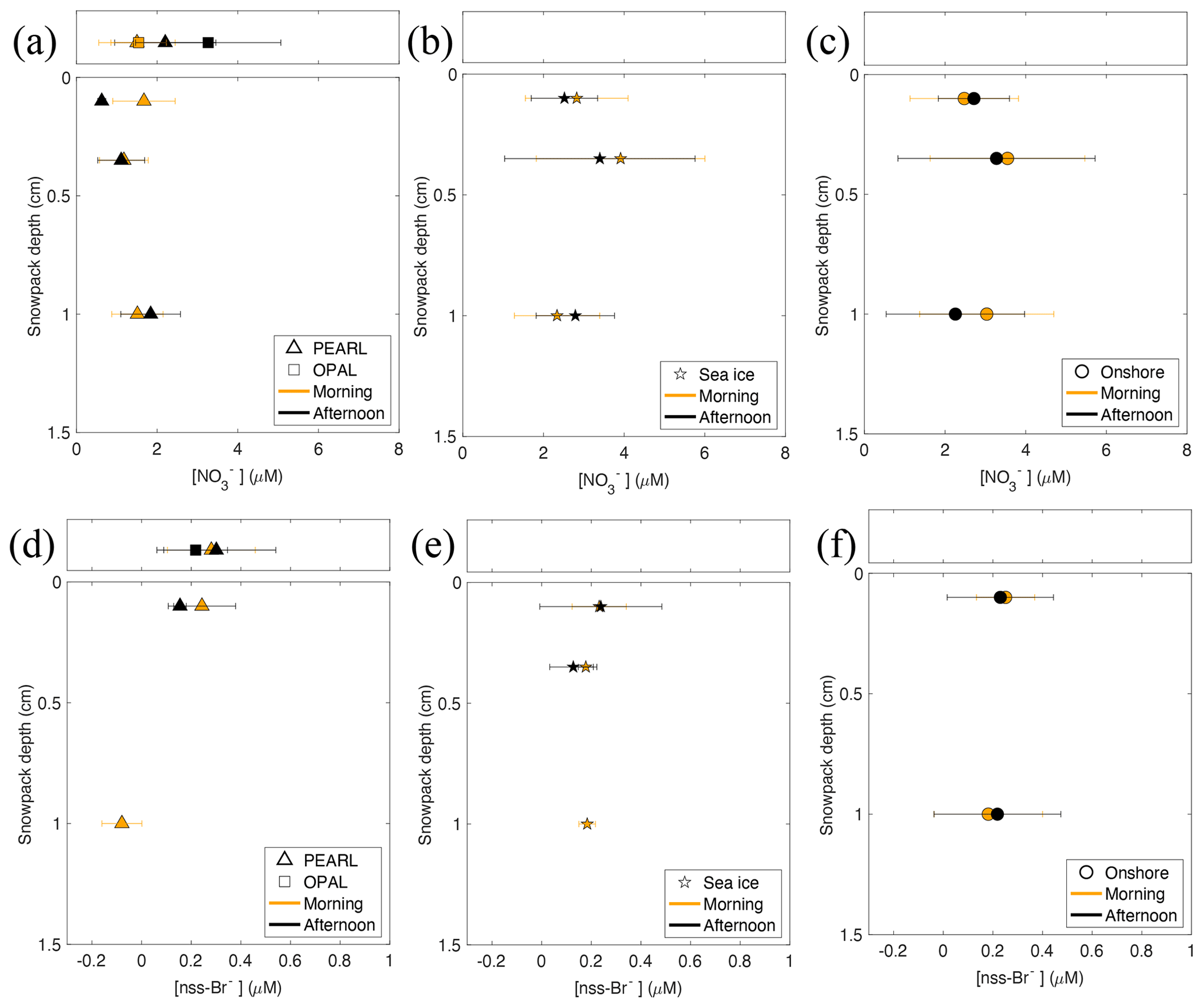
Figure 8 Morning and afternoon nss[Br⁻] and $\left[{\mathrm{NO}}_{\mathrm{3}}^{-}\right]$ from available snow samples collected between 3–16 March 2019. Note that only the mean values with p < 0.1 (in Table S6) are shown and used for the morning–afternoon difference calculation.

3.5 Morning versus afternoon nitrate and nss[Br⁻]

Compared to morning samples, afternoon samples at Eureka undergo 3–7 more hours of sunlight, which means photochemical loss of nitrate and bromide from snowpack may be enhanced as a result. The 2019 morning and afternoon concentrations of nitrate and nss[Br⁻] are shown in Fig. 8. The mean $\left[{\mathrm{NO}}_{\mathrm{3}}^{-}\right]$ for morning samples (at Sea ice and Onshore) is 3.02 ± 1.56 µM, which is larger than the afternoon mean of 2.79 ± 1.45 µM by 0.23 µM; at the PEARL site, the morning–afternoon difference is 0.48 µM (1.66 ± 0.48 µM in the morning vs. 1.18 ± 0.47 µM in the afternoon). However, from Fig. 8 and Table S6 we find the morning–afternoon differences are well within the error bars of the morning and afternoon samples and therefore cannot conclude that the small mean difference is a photochemical loss.

Snow bromide also shows a similar weak morning–afternoon difference; however the signals are not significant across all sampling sites. For example, at the Onshore site, the morning nss[Br⁻] in the first layer is 0.25 ± 0.12 µM (N=12, p < 0.001), which is larger than the afternoon 0.23 ± 0.21 µM (N=8, p = 0.019) by 0.02 µM; in the third layer the morning–afternoon difference is negative (−0.04 µM), calculated from the morning mean of 0.18 ± 0.22 µM (N=16, p = 0.005) and the afternoon mean of 0.22 ± 0.26 µM (N=12, p = 0.013) (Table S6). At the Sea ice site, the morning nss[Br⁻] in the first layer is smaller than the afternoon (by 0.01 µM); in the second layer, the morning nss[Br⁻] (0.18 ± 0.03 µM, N=10, p < 0.001) is larger than the afternoon (0.13 ± 0.09 µM, N=6, p = 0.022) by 0.02 µM. Based on the available data shown in Fig. 8, a mean morning–afternoon difference of 0.018 µM at sea level is derived. At PEARL, the morning–afternoon change is 0.07 µM (0.22 ± 0.13 µM vs. 0.15 ± 0.03 µM). Although the small positive morning–afternoon change is well in line with the possible daytime photochemical loss, due to the large error bars we cannot conclude that this signal is statistically meaningful. Therefore, we cannot claim that daytime photochemistry for snow bromide and nitrate is detected in this study.

Note that the tray sample $\left[{\mathrm{NO}}_{\mathrm{3}}^{-}\right]$ and nss[Br⁻] responded differently, with morning concentrations generally lower than their afternoon values. For example, at 0PAL the morning mean $\left[{\mathrm{NO}}_{\mathrm{3}}^{-}\right]$ for the tray samples (1.54 ± 0.69 µM, N=5, p = 0.007) is only half of the afternoon mean (3.27 ± 1.80 µM, N=8, p = 0.001). For bromide, at PEARL the morning mean nss[Br⁻] for the tray samples (0.28 ± 0.18 µM, N=8, p = 0.003) is also smaller than the afternoon mean (0.30 ± 0.24 µM, N=9, p = 0.005) by 0.02 µM. This finding is consistent with the vertical profiles of nitrate and bromide shown in Fig. 4c and e, where the tray sample $\left[{\mathrm{NO}}_{\mathrm{3}}^{-}\right]$ at 0PAL is 3.6 times the first-layer nitrate, and at PEARL it is 2.1 times the first-layer nitrate. Additionally, the tray sample nss[Br⁻] at 0PAL is 2.6 times the first-layer value. The enhancement of tray sample concentrations is likely due to the small amount of snow water collected by trays; the small addition of bromide deposited could increase its concentration much more than it would affect the large reservoir of surface snow.

3.6 Deposition flux of bromide and nitrate

The daily slopes of nitrate and bromide concentrations derived above can be used to calculate their deposition flux to snowpack following this new equation:

$$\begin{array}{}\text{(1)}& \mathrm{Flux}={\displaystyle \frac{A}{T}}{\sum }_{k=\mathrm{1}}^n{S}_k{H}_k{D}_k,\end{array}$$

where Flux is mean net deposition flux (deposition minus emission, in units of $\mathrm{molec}.{\mathrm{cm}}^{-\mathrm{2}}{\mathrm{s}}^{-\mathrm{1}}$) over the observational period from snow layer 1 to n, A is Avogadro's number of gas (6.02 × 10²³ $\mathrm{molec}.{\mathrm{mol}}^{-\mathrm{1}}$), T is seconds in a day (86 400 s d⁻¹), S_k is the derived daily slope in snow layer k (in µM d⁻¹), H_k is the corresponding snow layer depth (in cm), and D_k is snow density of the layer (in g cm⁻³).

In this study, n=3. A low snow density of 0.15 g cm⁻³ is used for the top two layers, and 0.3 g cm⁻³ is used for the third layer. For nitrate, mean slope values at sea level (from the Sea ice and Onshore sites) of 0.27, 0.2, and 0.07 µM d⁻¹ were used in the first, second, and third layers, respectively. Therefore, an integrated nitrate deposition flux of 2.6 × 10⁸ $\mathrm{molec}.{\mathrm{cm}}^{-\mathrm{2}}{\mathrm{s}}^{-\mathrm{1}}$ from the top 1.5 cm snow is obtained. At PEARL, the integrated deposition flux is negative (−1.0 × 10⁸ $\mathrm{molec}.{\mathrm{cm}}^{-\mathrm{2}}{\mathrm{s}}^{-\mathrm{1}}$) according to the mean slope of 0.0, −0.013, and −0.04 µM d⁻¹ in the three sub-layers. According to the statistical analysis results shown in Table S5, we can work out a mean slope error of 0.066 µM d⁻¹ at sea level and 0.019 µM d⁻¹ at PEARL. If we compare that to the average slopes derived of 0.28 µM d⁻¹ at sea level and −0.018 µM d⁻¹, we can work out relative errors of 37 % at sea level and 95 % at PEARL. Therefore, we have an integrated nitrate deposition flux of (2.6 ± 0.37) × 10⁸ $\mathrm{molec}.{\mathrm{cm}}^{-\mathrm{2}}{\mathrm{s}}^{-\mathrm{1}}$ at sea level and (−1.0 ± 1.06) × 10⁸ $\mathrm{molec}.{\mathrm{cm}}^{-\mathrm{2}}{\mathrm{s}}^{-\mathrm{1}}$ at PEARL. These results indicate that surface snow at sea level is a net sink of atmospheric nitrate, and at the hilltop it is a source of reactive nitrogen; however, the negative flux derived at PEARL has a large error bar, indicating the flux has a large uncertainty. Our derived nitrate deposition flux at sea level Eureka is close to the winter average flux of 2.7 × 10⁸ $\mathrm{molec}.{\mathrm{cm}}^{-\mathrm{2}}{\mathrm{s}}^{-\mathrm{1}}$ derived at Alert, Nunavut (Macdonald et al., 2017), and ∼ 4 × 10⁸ $\mathrm{molec}.{\mathrm{cm}}^{-\mathrm{2}}$ s⁻¹ at Svalbard (Björkman et al., 2013), justifying the method used in this work.

For bromide, the integrated deposition flux from R6 is 1.01 × 10⁷ $\mathrm{molec}.{\mathrm{cm}}^{-\mathrm{2}}{\mathrm{s}}^{-\mathrm{1}}$ at sea level, using a mean slope of 0.024, 0.016, and 0.0 µM d⁻¹ in the three sub-layers, respectively. At PEARL, the integrated flux is 7.9 × 10⁶ $\mathrm{molec}.{\mathrm{cm}}^{-\mathrm{2}}{\mathrm{s}}^{-\mathrm{1}}$. Similarly, from Table S5 we can derive a mean slope error of 0.0096 µM d⁻¹ at sea level and 0.0059 µM d⁻¹ at PEARL (for the top two layers). If we compare that to the average slope of 0.02 µM d⁻¹ at sea level and 0.015 µM d⁻¹ at PEARL, we have relative errors of 48 % at sea level and 39 % at PEARL. Therefore the integrated bromide flux is (1.01 ± 0.48) × 10⁷ $\mathrm{molec}.{\mathrm{cm}}^{-\mathrm{2}}{\mathrm{s}}^{-\mathrm{1}}$ at sea level and (0.79 ± 0.31) × 10⁷ $\mathrm{molec}.{\mathrm{cm}}^{-\mathrm{2}}{\mathrm{s}}^{-\mathrm{1}}$ at PEARL. This small vertical gradient strongly indicates that BrO concentrations (and total inorganic bromine species) at sea level and in the free troposphere are not significantly different at Eureka, which agrees with the conclusion in Bognar et al. (2020). This implies that either bromine at Eureka is mixed well in the lower troposphere (mainly during strong wind events with enhanced BrO) or local snowpack at sea level is not a large source of reactive bromine. As mentioned previously, from winter to early spring the Eureka boundary layer is very shallow and stratified in calm conditions; thus most of the time PEARL is in the free troposphere. Therefore, if local snowpack on sea ice in the fjord is a large source of reactive bromine, an enhanced deposition flux at sea level should be detected. In addition, previous work focusing on atmospheric chemistry has demonstrated that large BrO enhancement events observed in Eureka in early springtime are mostly transported via cyclones (Zhao et al., 2016, 2017; Yang et al., 2020). The transported bromine in association with storms means well-mixed bromine species from the surface up to the free troposphere (> 1 km), which explains the small vertical gradient of deposited bromine flux in this current work.

3.7 Bromine mass balance analysis

For gas-phase bromine (as a family), its concentration C_air in the air can be expressed as

$$\begin{array}{}\text{(2)}& {\displaystyle \frac{\mathrm{d}{C}_{\text{air}}}{\mathrm{d}t}}=P_{\text{air}}-{\displaystyle \frac{C_{\text{air}}}{{\mathit{\tau }}_{\text{air}}}},\end{array}$$

where P_air is the emission flux of reactive bromine from snowpack and τ_air is the lifetime of bromine species in the air. The second term $\frac{C_{\text{air}}}{{\mathit{\tau }}_{\text{air}}}$ on the right side represents removal of bromine from the air via deposition. At an equilibrium state, concentration C_air will reach a stable level (= P_air × τ_air). However, from Figs. 5c and 6c, we see a significant decreasing trend of BrO partial column, indicating the input term P_air is much smaller than the loss term $\frac{C_{\text{air}}}{{\mathit{\tau }}_{\text{air}}}$. If we take the linear decreasing slope of (−7.21 ± 0.38) × 10¹¹ $\mathrm{molec}.{\mathrm{cm}}^{-\mathrm{2}}{\mathrm{d}}^{-\mathrm{1}}$ in 2018 and (−3.03 ± 0.05) × 10¹¹ $\mathrm{molec}.{\mathrm{cm}}^{-\mathrm{2}}{\mathrm{d}}^{-\mathrm{1}}$ in 2019 and apply a 30 % partitioning of BrO in total gas bromine species as calculated by models (Legrand et al., 2016), then the loss rate of total bromine species is (−2.52 ± 0.13) × 10⁷ $\mathrm{molec}.{\mathrm{cm}}^{-\mathrm{2}}{\mathrm{s}}^{-\mathrm{1}}$ in 2018 and (−1.05 ± 0.02) × 10⁷ $\mathrm{molec}.{\mathrm{cm}}^{-\mathrm{2}}{\mathrm{s}}^{-\mathrm{1}}$ in 2019. The 2019 removal flux is in good agreement with the derived snow bromide deposition flux of (1.01 ± 0.48) × 10⁷ $\mathrm{molec}.{\mathrm{cm}}^{-\mathrm{2}}{\mathrm{s}}^{-\mathrm{1}}$, implying the snow bromide is a deposit of atmospheric gas-phase bromine.

In addition, the mathematical solution of Eq. (2) is an exponential function, which can be simplified to a linear function as long as τ_air is much larger than 1 d. The exponential fits to the BrO data give τ_air values of ∼ 17 d in 2018 and ∼ 42 d in 2019, which are about 2–10 times the model-derived global mean lifetimes of ∼ 10 d (von Glasow et al., 2004) and 4–5 d (Yang et al., 2005). Note that term τ_air in Eq. (2) should not be treated as actual lifetime of reactive bromine obtained in an isolated air mass. This is because polar atmosphere is an open system, over a long-term period (from weeks to months), the timescale of decay of atmospheric bromine may be enhanced by many factors including the heterogeneous reactivation or recycling of inactive bromine species on surface of particles. Therefore, the above derived τ_air values can be treated as a seasonal decay lifetime of polar atmospheric bromine.

Similarly, for snow bromide concentration C_snow, its time-dependent evolution can be expressed as

$$\begin{array}{}\text{(3)}& {\displaystyle \frac{\mathrm{d}{C}_{\text{snow}}}{\mathrm{d}t}}=P_{\text{snow}}-{\displaystyle \frac{C_{\text{snow}}}{{\mathit{\tau }}_{\text{snow}}}},\end{array}$$

where P_snow is the snow bromide input from the air, which equals the gas-phase bromine loss term $\frac{C_{\text{air}}}{{\mathit{\tau }}_{\text{air}}}$ in Eq. (2), and τ_snow is the lifetime of snow bromide. The second term $\frac{C_{\text{snow}}}{{\mathit{\tau }}_{\text{snow}}}$ on the right side represents release of snow bromide (via photochemistry), which equals the input term P_air in Eq. (2). At a photochemical steady state and under the assumption that snow bromide lifetime τ_snow does not change much during the measurement period, a constant C_snow = P_snow × τ_snow is expected. However, Fig. 6 indicates that C_snow increases linearly, suggesting the input term P_snow must be much larger than the loss term $\frac{C_{\text{snow}}}{{\mathit{\tau }}_{\text{snow}}}$ to fit a linear increasing trend as measured. This means the daytime photochemical release of bromide from the surface snow must be much smaller than the deposited bromide.

If we assume the net increase of bromide in the surface snow layer is roughly balanced by the release of reactive bromine from the whole snow column, then a rough bromine mass balance could be reached. This means the emission flux of reactive bromine from snowpack photochemistry is about the same as the deposited bromide flux of (1.01 ± 0.48) × 10⁷ $\mathrm{molec}.{\mathrm{cm}}^{-\mathrm{2}}{\mathrm{s}}^{-\mathrm{1}}$ at sea level. But this emission flux will balance the gas-phase bromine removal flux of (−1.05 ± 0.002) × 10⁷ $\mathrm{molec}.{\mathrm{cm}}^{-\mathrm{2}}{\mathrm{s}}^{-\mathrm{1}}$ and should result in a stable atmospheric bromine level rather than a decreased BrO trend as observed, unless the BrO partitioning in total bromine species decreases with time in early spring. Otherwise, we must conclude that deposition of bromide to surface snow is more likely “one-way” (or unidirectional). Namely, the photochemical release of reactive bromine from snowpack must be very weak and smaller than the derived deposition flux on the order of 1 × 10⁷ $\mathrm{molec}.{\mathrm{cm}}^{-\mathrm{2}}{\mathrm{s}}^{-\mathrm{1}}$.

3.8 Relationship between surface snow $\left[{\mathrm{NO}}_{\mathrm{3}}^{-}\right]$ and [Br⁻]

There are multiple sources of snowpack bromide and nitrate. For example, bromide may come from reactive bromine gases (such as HOBr, BrO and BrONO₂) and the terminal product HBr in both gas phase and particle phase. Due to the lack of in situ data, we cannot accurately quantify the contribution of HBr to snow bromide at Eureka. However, modelling work (focusing on Antarctic coastal Dumont d'Urville chemistry) indicates that reactive bromine species dominate total gaseous inorganic bromine. For example, gas-phase HOBr and BrO together account for ∼ $\mathrm{2}/\mathrm{3}$ of total inorganic bromine on average, and gas-phase HBr only accounts for 12 %. In austral spring (September–October), HBr partitioning is higher but does not exceed 25 % (from Fig. 14 of Legrand et al., 2016). Bromine may accumulate as gas-phase HBr when ozone depletion has terminated (Lehrer et al., 2004), but during the campaign period surface ozone rarely dropped below 2–3 ppbv (Figs. 5a and 6a); therefore, gas-phase HBr accounts for a small fraction of total inorganic bromine. In addition, airborne particles can take up gas-phase HBr from the air. Size-dependent aerosol data from both hemispheres indicate that the smallest particles (sub-micrometre size mode) are normally enhanced in Br⁻ (as compared to sea salt reference), while large-sized particles are slightly Br-depleted (Alvarez-Aviles et al., 2008; Legrand et al., 2016). Figure S7 shows that at the Onshore site surface snow sodium and bromide are not significantly correlated apart from in the third layer. At Sea ice, surface snow sodium and bromide are largely correlated but with $\left[{\mathrm{Br}}^{-}\right]/\left[{\mathrm{Na}}^{+}\right]$ ratios larger than the sea water ratio (∼ 0.0065) indicating that surface snow gains bromide from the air at Eureka. This is in line with the finding at coastal Alaska (Simpson et al., 2005). Moreover, the observed large bromide enhancement factor (> 10, Fig. 4g and Sect. 3.2) strongly indicates that bromide in surface snow is not related to sea salt. Thus, it is reasonable to make the assumption that nssBr⁻ mainly comes from reactive bromine species.

Relatively low nitrate concentrations of 0.1–8.2 µM were detected in Arctic sea ice (Clark et al., 2020); their isotope-based investigation of the origin of nitrate indicates that the atmospheric contribution accounts for 40 % or less of the sea ice nitrate, demonstrating the importance of atmospheric reactive nitrogen to sea ice nitrate. Our data indicate that there is no significant relationship between sodium and nitrate in surface snow, which is consistent with the finding for Alaska (Krnavek et al., 2012).

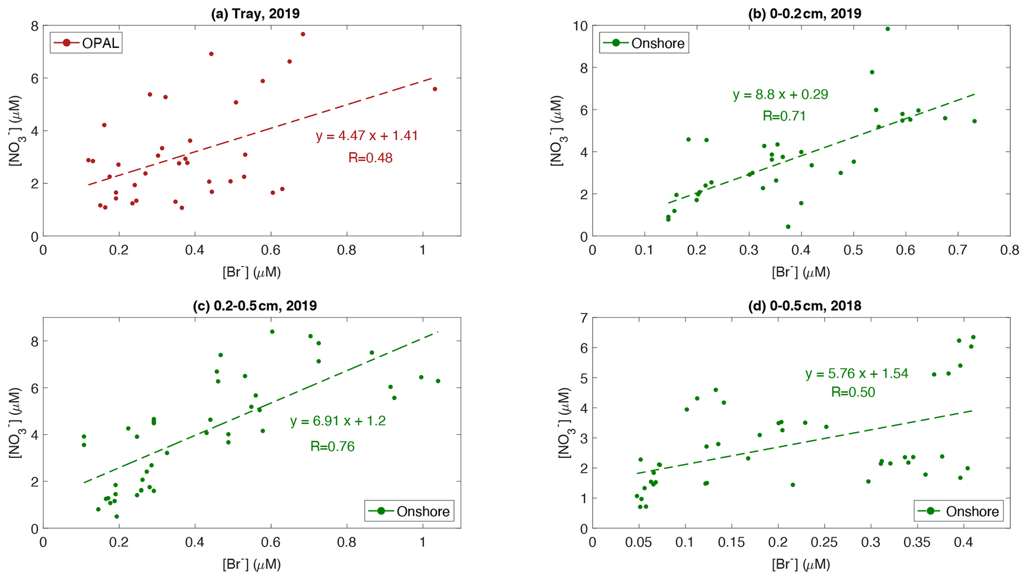
Figure 9 Scatter plot of surface snow nitrate versus bromide in (a) tray samples (2019), (b) 0–0.2 cm layer (2019), (c) 0.2–0.5 cm layer (2019), and (d) 0–0.5 cm layer (2018). Linear regressions and corresponding correlation coefficients R are given.

However, a significant relationship is found between surface snow $\left[{\mathrm{NO}}_{\mathrm{3}}^{-}\right]$ and [Br⁻] (Fig. 9) in tray samples at 0PAL, 0–0.2 cm, and 0.2–0.5 cm layer snow at the Onshore site (2019) and the top 0.5 cm snow at the Onshore site (2018), with an R value in the range of 0.4–0.7. This relationship remains when nss[Br⁻] is used in the analysis with a similar R of 0.23–0.66 (Fig. S8). In early spring, due to the small solar zenith angle, atmospheric OH is very low and the dominant pathway of oxidizing NO_x to form nitrate is likely via the chain Reactions (R1)–(R4). From the net reaction in Reaction (R5) we can see that without net consumption of bromine, NO_x and ozone can be effectively consumed, which means more than one NO_x molecule can be converted to nitrate per bromine atom. Figure 9 shows that the ratio of $\left[{\mathrm{NO}}_{\mathrm{3}}^{-}\right]/\left[{\mathrm{Br}}^{-}\right]$ ranges from 3.5–6.8, indicating that one molecule of bromide deposited to the surface is likely accompanied by 4–7 nitrate molecules, attributed to the fast recycling of gas-phase bromine species before they deposit to the surface snow. For the first time, we see field evidence on a timescale of one day showing this effect such as via Reactions (R1)–(R4). This finding further confirms previous conclusions regarding the role that reactive bromine plays in determining high-latitude atmospheric reactive nitrogen (e.g. Yang et al., 2005; Morin et al., 2008). Such a relationship can be detected in surface snow on sea ice due to the sea water effect on bromide as shown in Fig. S8. However, we do see a weak correlation between them at PEARL (not shown).

4 Discussion and implications for polar chemistry

It is reasonable to assume that a rough balance of bromine can be reached in both the atmosphere and the snowpack over the sea ice zone. However, once bromine-rich air masses transport from sea ice into inland tundra areas, the bromine budget balance breaks down. In particular, air starts to lose gas-phase bromine and snow begins to gain extra bromide from the air, as we observed at Eureka. However, if quick photochemical equilibrium is reached in surface snow, then we should see a stable bromide concentration in snow. The same goes for gas-phase bromine in the air. However, the significant decrease in BrO partial column in the lower troposphere and the increase in surface snow bromide strongly indicate that they do not reach a photochemical equilibrium state in early spring.

Snow nitrate can be directly photo-dissociated under sunlight, while snow bromide activation needs heterogeneous photochemistry. Therefore, photons are a necessary but not a sufficient condition for bromine recycling. For example, the heterogeneous reactions for snowpack bromide reactivation involve three transport steps: aerodynamics bring gas HOBr or ozone to the near-surface sub-layer, and the subsequent transport requires gas molecules to pass through the quasi-laminar boundary layer before they can eventually be absorbed by snow particles. It has been shown that the above three processes vary greatly, depending on the depositing species and surface characteristics (Wu et al., 1992). The bromide loss rate from surface snow is somehow rate-limited by the deposition flux of hypohalous acid such as HOBr or ozone. This could be one reason for the possible weak emission flux of snow reactive bromine.

Snowpack is thought to be a highly permeable material, meaning gases and fine aerosols could penetrate into deep layers (Harder et al., 1996; Björkman, et al., 2013) due to the exchange of air with the atmosphere (Sturm and Johnson, 1991; Albert and Hardy, 1995; Colbeck, 1997; Albert et al., 2002). However, our data show that most deposited species were in the top 0.5 cm layer. For example, at sea level nitrate slopes reduce significantly from the first-layer mean of 0.26 µM d⁻¹ to the second-layer mean of 0.20 µM d⁻¹ and third-layer mean of 0.07 µM d⁻¹. A similar trend is also obtained for nss[Br⁻] slopes, with the first-layer slope of 0.023, the second-layer slope of 0.014, and the third-layer slope of 0.0 µM d⁻¹. These results indicate deposited nitrate and bromide are largely confined to the skin layer. The fog-related bromide and nitrate enhancements are only found in the top two layers (< 0.5 cm), which agrees with conclusions of Domine et al. (2004), who state that the aerosol effect on snow ion concentrations is limited to the top few centimetres. In extreme conditions, applying the above derived absolute nitrate deposition flux (0.632 µM d⁻¹) and absolute nss[Br⁻] deposition flux (0.064 µM d⁻¹) to all three layers allows for a nitrate deposition flux of 1.65 × 10⁹ $\mathrm{molec}.{\mathrm{cm}}^{-\mathrm{2}}{\mathrm{s}}^{-\mathrm{1}}$ and a bromide deposition flux of 1.72 × 10⁸ $\mathrm{molec}.{\mathrm{cm}}^{-\mathrm{2}}{\mathrm{s}}^{-\mathrm{1}}$ to be calculated. These may represent the upper limits of the deposition fluxes of nitrate and bromine.

As shown above, the uncertainty of the bromide measurements is larger in the third layer and on sea ice, where the accumulated salts and sea water make the non-sea-salt bromine signals harder to detect. We also do not have samples from deeper snow layers (> 1.5 cm); therefore, our measurements may underestimate the deposition flux of nitrate and bromide. Although the snow e-folding depth (light attenuation) at Eureka was not measured, previous measurements at other polar sites indicate that it varies from a shallow 2–5 cm (Erbland et al., 2013) to a deep 10–20 cm (France et al., 2011) in Antarctica. At Cambridge Bay, Canada, an e-folding depth of 16 cm was reported in March snowpack (Xu et al., 2016). Therefore, the loss of nitrate and bromide via photochemistry or the release of reactive nitrogen and bromine may come from a deeper snow layer, which we have no data to confirm.

The method used to derive the deposition flux of nitrate and bromide is different from the instrument-based measurements of gas reactive nitrogen and bromine, and the method applied could not resolve short-term (< 1 d) fluxes. Therefore, the derived fluxes only represent an average over the campaign period (3–4 weeks). In addition, the success is largely dependent on the choice of sampling location, ideally where the snowpack on sea ice and inland is less disturbed by other bromine sources such as open leads, polynyas, and sea spray. Therefore, this method may not work well in areas where sea ice has a significant amount of mobility, with sea ice opening and closing frequently. The conclusions derived in this study may only be representative of local characteristics, as sea ice conditions at Eureka are quite different from those in the central Arctic (Shupe et al., 2022). However, the physical and chemical processes involved in bromide deposition and reactive bromine release may remain the same across locations. To confirm this, a more comprehensive field campaign under typical Arctic sea ice conditions is needed.

Note that the lifetime of an individual reactive bromine species such as BrO and HOBr is short (only a few minutes) under sunlight. However, as a family, the timescale of decay of inorganic bromine species in the atmosphere will be much longer, e.g. from the model estimated global mean of 4–10 d (Yang et al., 2005; von Glasow et al., 2004) to this study estimation of up to ∼ 40 d in early spring at Eureka. For nitrogen oxides (NO_x), the lifetime in Arctic springtime is 2–6 d (Stroud et al., 2003). It is important to note that within a stable boundary layer, the typical time needed for a surface signal to reach the upper layer is 7–30 h (Stull, 1988). Therefore, within the 1 d timescale selected for snow sampling, emitted reactive bromine and nitrogen should have sufficient time to mix well in the boundary layer and reach a quasi-equilibrium state with other processes, including deposition and photochemistry.

5 Summaries and conclusions

Skin layer snow salinity at the inland site has a double-peak distribution, with the first peak at 0.001–0.002 psu corresponding to the precipitation effect and the second peak at 0.01–0.04 psu likely due to the salt accumulation effect. Snow salinity on sea ice has a triple-peak distribution, and the third peak at 0.2–0.4 psu is clearly related to the sea water effect due to the upward migration of brine on sea ice. The presence of an iceberg in the valley could significantly dilute ice and column snow salinity as observed in 2019 samples.

Based on daily surface snow sampling in the Canadian high Arctic, an integrated spring nitrate deposition flux of (2.6 ± 0.37) × 10⁸ $\mathrm{molec}.{\mathrm{cm}}^{-\mathrm{2}}{\mathrm{s}}^{-\mathrm{1}}$ has been derived from the top 1.5 cm snow in the fjord of Eureka. At the top of the hill (PEARL Ridge Lab, ∼ 600 m), nitrate deposition flux is negative (−1.0 ± 1.06) × 10⁸ $\mathrm{molec}.{\mathrm{cm}}^{-\mathrm{2}}{\mathrm{s}}^{-\mathrm{1}}$) indicating snow is losing nitrate in early spring. Integrated bromide deposition flux at sea level is (1.01 ± 0.48) × 10⁷ $\mathrm{molec}.{\mathrm{cm}}^{-\mathrm{2}}{\mathrm{s}}^{-\mathrm{1}}$; at the hilltop, the deposition flux is (0.79 ± 0.31) × 10⁷ $\mathrm{molec}.{\mathrm{cm}}^{-\mathrm{2}}{\mathrm{s}}^{-\mathrm{1}}$. The small vertical gradient between the boundary layer and the free troposphere indicates local snowpack is a weak reactive bromine emission source. On the contrary, the large vertical gradient in nitrate deposition flux strongly indicates that snowpack at sea level is a large emission source of reactive nitrogen. In addition, the bromide deposition flux at sea level is more than an order of magnitude smaller than the nitrate deposition flux.

Due to the large error bars, we could not derive robust conclusions regarding whether snow nitrate and bromide in the morning samples were generally higher than in the afternoon samples. We therefore could not derive any conclusion regarding snowpack photochemistry. BrO partial column (0–4 km) data measured by MAX-DOAS show a clear decreasing trend in early spring, which generally agrees with the derived surface snow bromide deposition flux, indicating that bromine in Eureka atmosphere and surface snow did not reach a photochemical equilibrium state. Through the mass balance analysis, we conclude that the average emission flux from snow over the campaign period should be smaller than the average bromide deposition flux of ∼ 1 × 10⁷ $\mathrm{molec}.{\mathrm{cm}}^{-\mathrm{2}}{\mathrm{s}}^{-\mathrm{1}}$, which is an order of magnitude smaller than previously measured emission flux of 0.7–12 × 10⁸ $\mathrm{molec}.{\mathrm{cm}}^{-\mathrm{2}}{\mathrm{s}}^{-\mathrm{1}}$ (Custard et al., 2017). Note that the net mean fluxes observed do not completely rule out larger bidirectional fluxes over shorter timescales.

Due to the lack of field data on typical Arctic sea ice, we cannot conclusively say whether the result obtained in this study is a local characteristic or can be extended to a broad Arctic area. However, our finding is in line with the conclusion made by Legrand et al. (2016) that snowpack bromine emission is not important over the Antarctic Plateau.

Additionally, we find skin layer snow nitrate and bromide are significantly correlated with a $\left[{\mathrm{NO}}_{\mathrm{3}}^{-}\right]/\left[{\mathrm{Br}}^{-}\right]$ ratio of 4–7, indicating reactive bromine could effectively accelerate NO_x-to-nitrate conversion. This is the first time such an effect has been seen on a timescale of 1 d. This also reinforces the importance of reactive bromine in polar and high-latitude reactive nitrogen budgets and its atmospheric oxidizing capacity.