Influences of sudden stratospheric warmings on the ionosphere above Okinawa

We analyzed the ionosonde observations from Okinawa (26.7° N, 128.1° E; magnetic latitude: 17.0° N) for the years from 1972 to 2023. Okinawa is in the northern low-latitude ionosphere, where the influences of sudden stratospheric warmings (SSWs) on the ionosphere are expected to be stronger than in the mid- and high-latitude ionospheres. We divided the dataset into winters with major SSWs in the Northern Hemisphere (SSW years) and winters without major SSWs (no-SSW years). During the SSW years, the daily cycle of the F2-region electron density maximum (NmF2) is stronger than in the no-SSW years. The relative NmF2 amplitudes of solar and lunar tidal components (S₂, O₁, M₂, MK₃) are stronger by 3 % to 8 % in the SSW years than in the no-SSW years. The semidiurnal amplitude, averaged across 29 SSW events, has a significant peak at the central date of the SSW (epoch time 0 of the composite analysis). The SSW influence is not strong: the semidiurnal amplitude is about 38.2 % in the SSW years and about 34.0 % in the no-SSW years (relative to the NmF2 of the background ionosphere). However, there is a sharp decrease in the amplitude of about 10 % after the SSW peak is reached. The amplitude of the diurnal component does not show a single peak at the central date of the SSW. We present the maximal semidiurnal amplitudes of the SSWs since 1972. The SSW of 31 December 1984 has the strongest amplitude (162 %) in the ionosphere above Okinawa (with a high geomagnetic activity, Ap, of 37 nT). The most surprising finding of the study is the strong lunar tides with relative amplitudes of about 10 % and the discovery of a terdiurnal lunar tide (5 %) in the NmF2 during the SSW years. The periods of the ionospheric lunar tides align with the periods of ocean tides and lunisolar variations in the atmosphere.

1 Introduction

It has been observed and simulations have shown that sudden stratospheric warmings (SSWs) affect the whole atmosphere and ionosphere of the Earth (Pedatella et al., 2018). Sudden stratospheric warmings can be divided into minor and major SSWs (McInturff, 1978). Contrary to minor SSWs, major SSWs cause a reversal of the stratospheric polar vortex from eastward to westward flow in the middle stratosphere. The central date of an SSW (SSW onset) is defined as the time point of the reversal of the stratospheric zonal wind at 10 hPa (about 30 km altitude) and at 60° N latitude. There are also SSWs in the Southern Hemisphere, but they are quite rare, while the major SSWs in the Northern Hemisphere occur every 1–2 years.

In the present study, we only consider the influence of major SSWs in the northern hemispheric winter on the ionosphere. The reversal of the stratospheric polar vortex is caused by planetary wave breaking. In addition, severe disturbances, splitting, or breakdown of the stratospheric polar vortex are observed during SSW events. A major SSW is associated with a rapid increase in the polar stratospheric temperature and a reversal of the vortex from eastward to westward flow for at least 5 d (Matsuno, 1971; Schoeberl, 1978; McInturff, 1978; Matthewman et al., 2009).

It is well established that variations in polar stratospheric winds can affect mesospheric temperatures through changes in the filtering of gravity wave fluxes, which drive residual circulation in the mesosphere. SSWs are often associated with mesospheric cooling since the breakdown of the stratospheric polar vortex leads to an enhanced gravity wave flux from below into the mesosphere, with associated upwelling and adiabatic cooling of the mesosphere. In the weeks after the SSW onset, an elevated stratopause appears in the polar mesosphere. The elevated stratopause slowly descends over several weeks to about 50 km in altitude (Zülicke and Becker, 2013).

The present knowledge of the influences of SSWs on the ionosphere has been reviewed by Goncharenko et al. (2021). Particularly, the upward-propagating solar and lunar tides could have different propagation conditions due to SSW effects on the middle atmosphere. The excitation, propagation, and dissipation of solar and lunar tides have been described by means of the classical tidal theory, which linearizes the primitive equations, providing Laplace's tidal equations (Lindzen and Chapman, 1969). The ionospheric effect of an SSW is most obvious in the low-latitude ionosphere, where a strongly amplified semidiurnal pattern in total electron content, equatorial vertical ion drift, and the equatorial electrojet have been observed (Goncharenko et al., 2021, 2013; Yamazaki et al., 2012). Yamazaki et al. (2012) also found that the geomagnetic lunar tide at the geomagnetic equator is enhanced in 70 % of the SSW events. However, the role of lunar and solar tidal variability in the generation of the ionospheric effects of SSWs is still under investigation. The relative amplitudes of the semidiurnal lunar tide M₂ (period 12.42 h) are about 5 % at low latitudes relative to the mean background electron density (Forbes and Zhang, 2019; Pedatella, 2014). Forbes and Zhang (2019) also noted the importance of the quasi-diurnal lunar tide O₁ (period 25.82 h) in the ionosphere. At mid-latitudes, the SSW effects on the ionosphere are seen more as an increase in the mean electron density than as an increase in ionospheric tidal variability (Mošna et al., 2021).

The present study investigates the ionospheric effects of major SSWs at the northern border of the low-latitude ionosphere. We take advantage of the long-term series of peak ionospheric electron density (NmF2), observed by an ionosonde in Okinawa. Kalita et al. (2015) analyzed the seasonal and diurnal variability in NmF2 in Okinawa and the influence of the equatorial ionization anomaly (EIA) at this location. The attribution of the ionospheric changes to SSW events is relatively difficult since the ionospheric effect can be delayed or advanced by several days with respect to the central date of the SSW. Thus, a composite analysis of many SSW events is required to characterize the average behavior of the SSW-induced ionospheric changes. In addition, the solar and lunar tides are modulated by mesospheric winds. The mesospheric wind field is still not well observed but is necessary for ionospheric predictions (Harvey et al., 2022). It has been observed that the migrating diurnal solar tide at the Equator is reduced in amplitude by SSW events (Siddiqui et al., 2022; Hocke, 2023). The ionosonde series allows for the discussion of variability in solar and lunar tides during the SSW events. It remains an open question whether solar or lunar tidal variability is more important for the ionospheric effects of SSWs. The long-term ionosonde series recorded at several locations in the world also give us a unique opportunity to study historical SSW events of the 1950s or even earlier, when stratospheric observations were rare but ionospheric observations were already common.

2 Dataset and data analysis

Ionograms record tracings of high-frequency (HF) radio pulses reflected in the ionosphere. They are produced by the vertical-incidence ionospheric sounder (ionosonde) in Okinawa, Japan (26.7° N, 128.1° E; magnetic latitude: 17.0° N). The sounding frequency is swept from 1 to 30 MHz. Ionograms are obtained at regular intervals of 15 min and contain several important factors, such as the ordinary-mode critical frequency or maximum reflection frequency of the ionospheric F2 layer (foF2). In the present study, we use the manually scaled ionospheric parameter foF2, which is provided with a time resolution of 1 h from 1972 to 2023 by the World Data Center for Ionosphere and Space Weather at the National Institute of Information and Communications Technology in Tokyo.

The parameter foF2 is closely related to the maximum electron density (NmF2) of the ionospheric F2 layer, as shown by

$$\begin{array}{}\text{(1)}& \mathrm{NmF}\mathrm{2}=\mathrm{1.24}\times {\mathrm{10}}^{\mathrm{10}}(\mathrm{foF}\mathrm{2}{)}^{\mathrm{2}},\end{array}$$

where NmF2 is in cubic meters and foF2 is in megahertz (Davies, 1990; Chuo, 2012). In the present study, we mainly analyze the time series of NmF2. The relative amplitudes are computed with respect to a temporal average of NmF2, which is either the mean of the depicted time interval or a 60 d low-pass-filtered series of NmF2.

For the data analysis, we used a digital non-recursive, finite-impulse-response band-pass filter. Zero-phase filtering is ensured by processing the time series in forward and reverse directions. A Hamming window was selected for the filter. The number of filter coefficients corresponds to a time window of 3 times the central period, meaning the band-pass filter has a fast response time to temporal changes in the data series. The variable choice of the filter order permits the analysis of wave trains with a resolution that matches their scale. The band-pass cutoff frequencies are at $f_{\mathrm{c}}=f_{\mathrm{p}}\pm \mathrm{10}\mathit{\%}{f}_{\mathrm{p}}$, where f_c is the cutoff frequency and f_p is the central frequency. For the semidiurnal variation, the cutoff frequencies are 1.8 and 2.2 cycles per day (cpd). Further details about the band-pass filtering are provided by Studer et al. (2012). In the case of the 60 d low-pass filter, we used the cutoff frequencies of 0 and 1 cycle per 60 d.

For the case study of the SSW of 6 January 2013, we compare the Okinawa ionosonde data with data from the ionosonde for Wuhan (30.5° N, 114.4° E). The Wuhan ionograms have a time resolution of 15 min, and the foF2 values are automatically determined.

The composite analysis is limited to major SSWs during the northern hemispheric winter. The central date of a major SSW is defined as the date when the eastward wind changes to westward wind at 10 hPa, northward of 60° N (McInturff, 1978). The central date marks the onset time of the major SSW and is used as the timing mark for the composite analysis of major SSWs (Hocke et al., 2015). Of course, there are other processes in the mesosphere which may introduce an SSW or follow the SSW onset. For example, an elevated stratopause can be observed in the polar region in the weeks after the SSW onset (Manney et al., 2008).

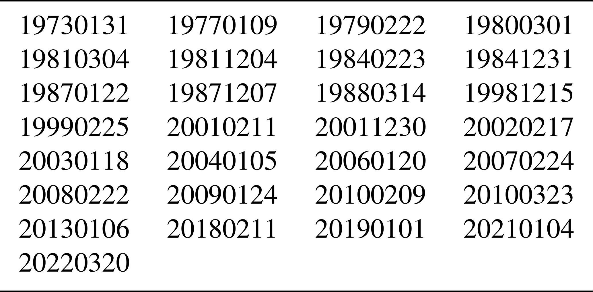
Palmeiro et al. (2023) determined the central dates of major SSWs using the zonal wind data from the fifth-generation European Centre for Medium-Range Weather Forecasts (ECMWF) atmospheric reanalysis (ERA5; Hersbach et al., 2020). Using Table 1 from Palmeiro et al. (2023), we obtained about 31 central dates of major SSWs from 1972 to 2023 (selected ionosonde series for Okinawa) that met the U60 criterion (reversal of zonal wind U at 60° N). Since Table 1 from Palmeiro et al. (2023) ends in January 2021, we added the major SSW of 20 March 2022 (Vargin et al., 2022). The list of central dates of the 29 SSW events used in the present study is shown in Table 1.

Table 1 Central dates of the 29 selected major SSWs in the Northern Hemisphere from 1973 to 2022. Due to some data gaps in the ionosonde series, we could not use all SSW events during this time interval as listed by Palmeiro et al. (2023).

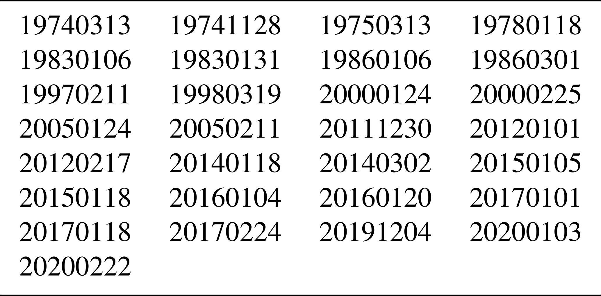
We also use a list of “no-SSW events” with central dates from December to March in northern hemispheric winters from 1974 to 2020 when no major SSW occurred. We selected the no-SSW events close to the SSW years in order to minimize the differences in solar activity and geomagnetic activity between the SSW years and no-SSW years. Thus, we did not include no-SSW events during the large gap of SSW events in the 1990s. The list of the 29 central dates of the no-SSW events is shown in Table 2.

Table 2 List of our arbitrary central dates of 29 “no-SSW events” from 1974 to 2020. These dates were used for the composites of the “no-SSW years”. Since there were not so many no-SSW years, we often put several events into 1 year.

The mean geomagnetic activity (Ap) was 12.0 nT in the selected no-SSW years and 11.7 nT in the selected SSW years. In terms of solar activity, the solar radio flux at 10.7 cm (F10.7) was 122 sfu (solar flux units) in the SSW years and smaller (112 sfu) in the no-SSW years. It is possible that SSW years have different conditions (e.g., solar activity, El Niño–Southern Oscillation (ENSO) activity) compared to no-SSW years. We performed a composite analysis for F10.7 and Ap and found no significant changes at epoch time 0 (SSW onset time). The composite lines were flat. Thus, we are sure that the SSW-induced characteristics of the NmF2 composites in the present study are not influenced by solar or geomagnetic activity.

For the spectral analysis of the solar and lunar tides in NmF2, we calculated the fast Fourier transform (FFT) spectrum of the relative NmF2 variations comprising the data from 5 weeks before the central date to 5 weeks after the central date of the SSW. This data segment was folded with a Hamming window. To enhance the frequency resolution, we used zero padding (4 years of zeros at the beginning and at the end of the data segment). The spectral analysis and the calculation of the relative amplitude were tested and calibrated using an artificial sine wave of a known amplitude and frequency. The length of the data interval (10 weeks) is sufficient for separating the solar and lunar tidal components, which we have verified by applying the same data analysis procedure to artificial sine waves.

2.1 Results

We start with the case study of the major SSW of 6 January 2013. Figure 1 shows the observed NmF2 from Okinawa and Wuhan from 5 d before the SSW onset to 15 d after the SSW onset. Obviously, the daily cycle is quite different at both stations, though the stations differ in latitude by just 3.8°. In addition, it is difficult to see a significant change in NmF2 which could be related to the SSW event.

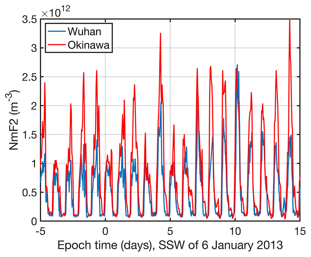
Figure 1 Time series of NmF2 for Okinawa (red) and Wuhan (blue) before and after the major SSW of 6 January 2013 (epoch time 0 corresponds to 6 January 2013).

However, Goncharenko et al. (2013) noted a strong amplification of the semidiurnal cycle in terms of vertical ion drift and total electron content (TEC) at the magnetic equator. This amplification of the semidiurnal pattern reached its maximum from 15 to 19 January 2013, which corresponds to an epoch time of 9 to 13 d. The maximal values of the upward ion drift were between 30 and 43 m s⁻¹ (Goncharenko et al., 2013). Thus, we applied a 12 h band pass to the ionosonde data from Okinawa and Wuhan. Figure 2 shows the relative amplitude of the semidiurnal cycle of NmF2. The relative amplitude is calculated with respect to the background mean of NmF2 averaged over an epoch time of −30 to 50 d. The amplitude curves align well for Okinawa and Wuhan. Both curves show a maximum at an epoch time of 10 d, which corresponds to 16 January 2013. This maximum of the semidiurnal cycle of NmF2 aligns well with the date of the maximum amplification of the semidiurnal pattern in vertical ion drift and TEC at the magnetic equator that was reported by Goncharenko et al. (2013). Coincidently, the semidiurnal tide of the mesospheric wind at middle and high northern latitudes was enhanced, as observations and simulations showed (van Caspel et al., 2023; Stober et al., 2020).

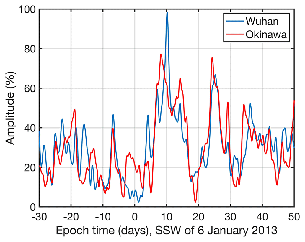
Figure 2 Time series of the relative amplitude of the semidiurnal cycle of NmF2 for Okinawa (red) and Wuhan (blue) before and after the major SSW of 6 January 2013. There is a maximum at an epoch time of 10 d, which is when the largest SSW effect was observed at the magnetic equator (Goncharenko et al., 2013).

The case study of 6 January 2013 motivated us to conduct a statistical study of the SSW effects in the semidiurnal cycle of the critical frequency foF2 from 1972 to 2023 in Okinawa. We start with foF2 since the composite shows a clearer effect than that for NmF2. The difference is possibly due to the fact that the average of a series of numbers (foF2)_i (i is the number of SSW events) has a different behavior than the average of the corresponding series of quadratic numbers (foF2²)_i in the composite of NmF2. Thus, the shapes of the composite curves are different for foF2 and NmF2.

The foF2 series is band-pass-filtered at a central frequency of 2 cpd, which correspond to the semidiurnal cycle. The amplitude series of the semidiurnal cycle is used for a composite analysis in which we added 29 SSW events to a composite. Figure 3 shows the result, which is averaged as a 14 d moving average. Obviously, there is a significant peak at epoch time 0, which is when we calculate the composite of the SSW years (red curve). The thin lines indicate the standard error in the composite. On the other hand, the peak at epoch time 0 disappears when we compute the composite of the no-SSW years (blue curve). There is also a seasonal variation in the amplitude since the central dates of the SSWs are always in the northern hemispheric winter (December to March) when the diurnal and semidiurnal variations in foF2 are maximal (Zolotukhina et al., 2011). The foF2 values are on average higher in the SSW years compared to the no-SSW years. This is due to a higher F2 peak electron density in the SSW years because of a higher solar activity in these years (F10.7 = 122 sfu in the SSW years, and F10.7 = 112 sfu in the no-SSW years). The geomagnetic index (Ap) is on average 11.7 nT in the SSW years and 12.0 nT in the no-SSW years.

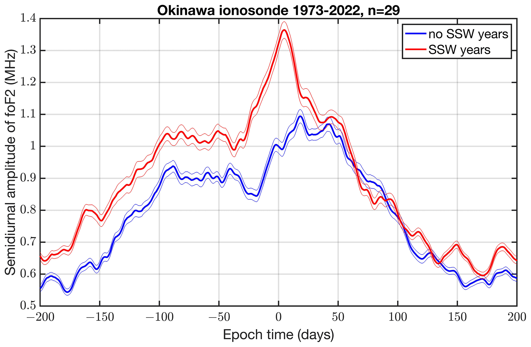
Figure 3 Composite of the amplitude of the semidiurnal cycle of foF2 in Okinawa for the SSW years (red) and no-SSW years (blue). The curves are averaged as a 14 d moving average. The thin lines denote the standard errors. In total, the composite consists of 29 SSW events from 1973 to 2022.

In the following, we will analyze the relative variations in the NmF2 series. First, the NmF2 series is filtered with a 60 d low-pass filter in order to obtain a background series. Then, the relative variations in NmF2 are calculated with respect to the background series of NmF2. The relative variations in NmF2 are band-pass-filtered at a central frequency of 2 cpd, corresponding to the semidiurnal cycle. The relative amplitude series of the semidiurnal cycle is used for a composite analysis in which we added 29 SSW events to a composite. Figure 4 shows the result, which is averaged as a 14 d moving average. Obviously, there is a significant peak at epoch time 0, which is when we calculate the composite of the SSW years (red curve). On the other hand, the peak at epoch time 0 disappears when we compute the composite of the no-SSW years (blue curve). Generally, the SSW effect is not as obvious as for foF2. Figure 4 shows an increase in the relative amplitude from 34.0 % (no-SSW years) to 38.2 % (SSW years). The occurrence of the peak just after epoch time 0 is a strong indication that the ionospheric effect is indeed related to the SSW onset. Please also note the sharp decrease in the amplitude of about 10 % after the SSW peak at epoch time 0 was reached. We did not find such a peak when we performed the composite analysis for the diurnal variation.

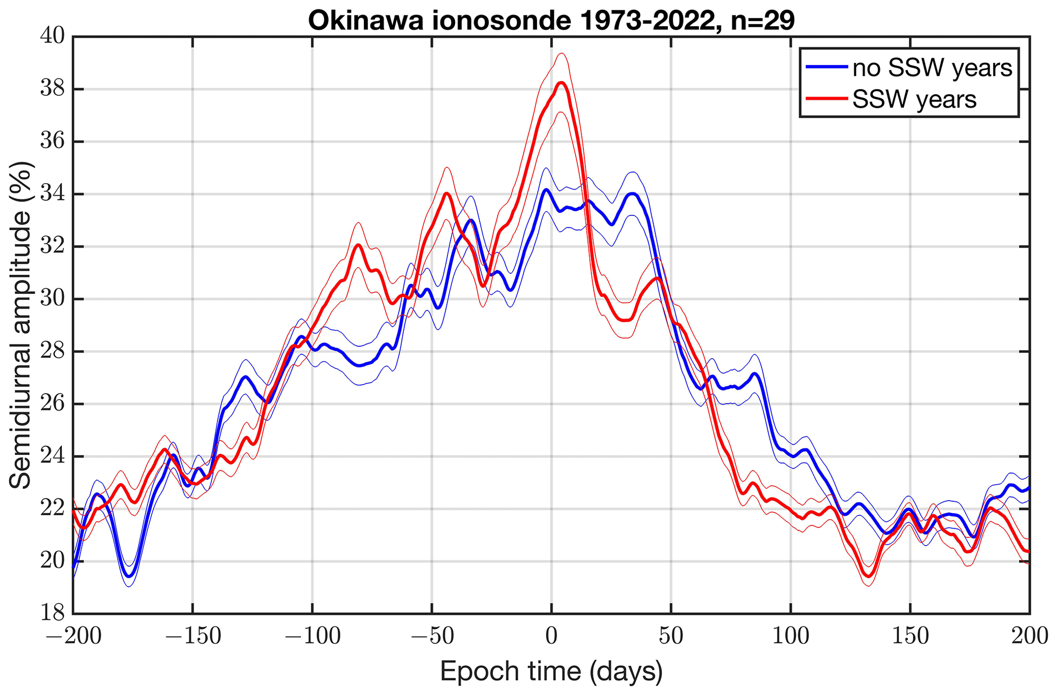
Figure 4 Composite of the relative amplitude of the semidiurnal cycle of NmF2 in Okinawa for the SSW years (red) and no-SSW years (blue). The curves are averaged as a 14 d moving average. The thin lines denote the standard errors. In total, the composite consists of 29 SSW events from 1973 to 2022.

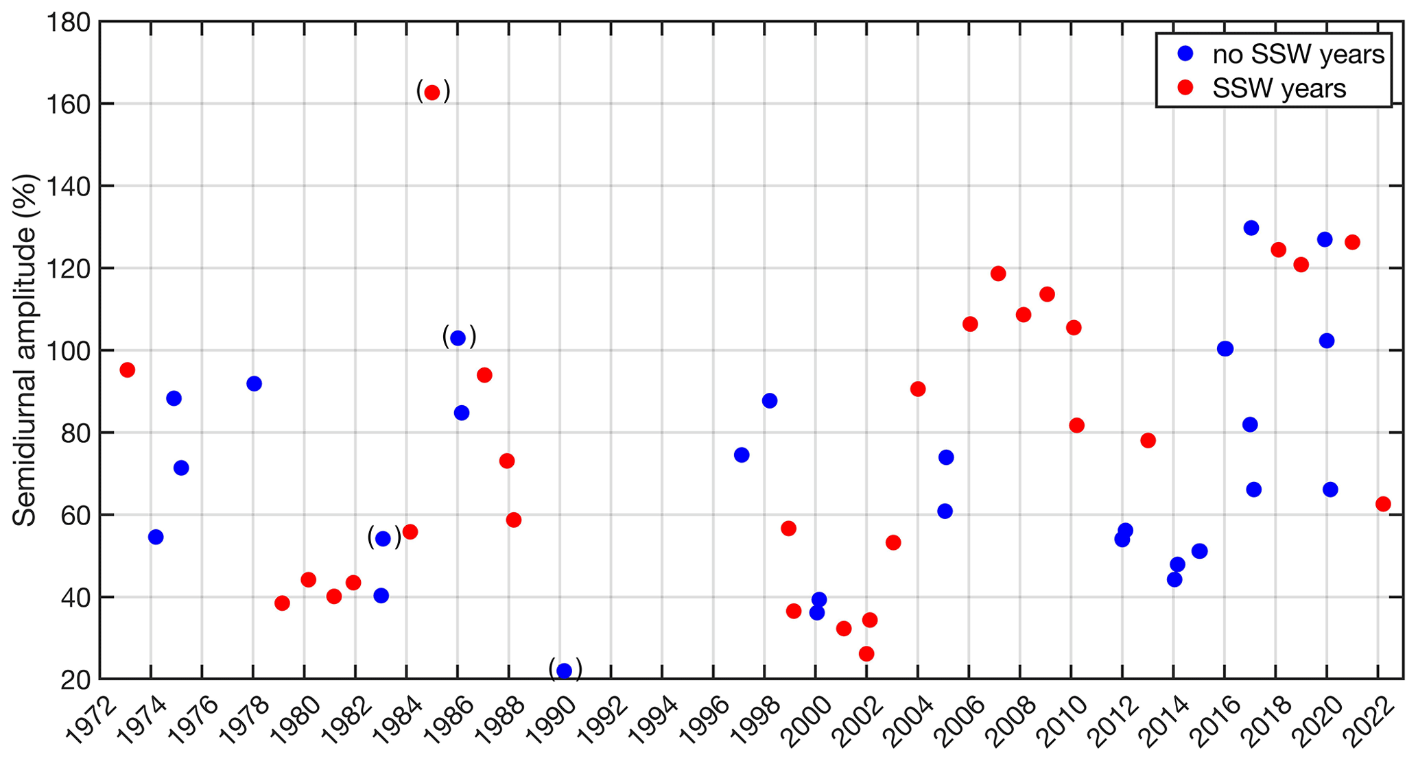
Figure 5 Time evolution of the maximum relative amplitude of the semidiurnal cycle of NmF2 in Okinawa for the SSW years (red) and no-SSW years (blue). The maximum is taken from 2 weeks before the central date to 2 weeks after the central date of a major SSW. The parentheses around four symbols indicate a high geomagnetic activity of Kp > 4 or Ap > 27 nT.

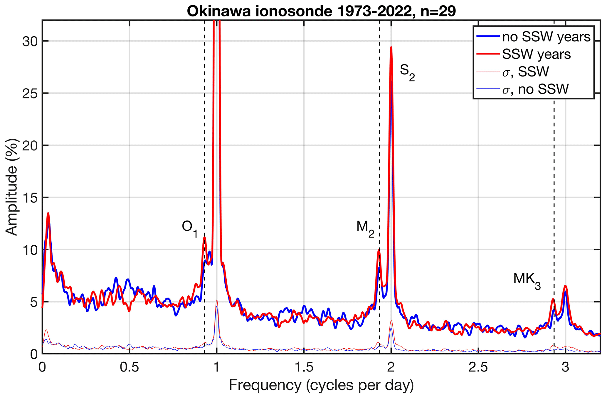
Figure 6 Composite of FFT spectra (time interval: 5 weeks before the SSW to 5 weeks after the SSW) for the SSW years (red) and no-SSW years (blue). The lunar components O₁, M₂, and MK₃ are indicated by the vertical dashed lines for the periods 25.82, 12.42, and 8.18 h. The solar and lunar components in the ionosphere above Okinawa are enhanced during the SSW years (composite of 29 SSW events). Please see the text for information about the S₁ peaks. The standard errors σ in the spectra are indicated by the thin lines at the bottom.

It is also interesting to study the time series of the maximum relative amplitudes of the semidiurnal cycle of NmF2. The maximum of the relative amplitude from 2 weeks before the central date to 2 weeks after the central date of the SSW is taken. Figure 5 shows the time evolution of the maximum relative amplitude of the semidiurnal cycle since 1972 for the SSW years and no-SSW years. It is evident that no-SSW years can also experience large amplitudes in the semidiurnal cycle. On average, the relative amplitudes are 70 % in the no-SSW years and 78 % in the SSW years. The largest amplitude occurred for the SSW of 31 December 1984 (about 162 %). However, the geomagnetic activity was quite high (Ap = 37 nT) for this event, meaning the amplification of the semidiurnal cycle could be due to geomagnetic activity in this case. On the other hand, Fig. 5 contains three other events for the no-SSW years with high geomagnetic activity, and these three cases do not show a strong amplification of the semidiurnal amplitude. Generally, the attribution of an amplitude increase to an individual SSW event is not easy because of the high variability in the ionosphere.

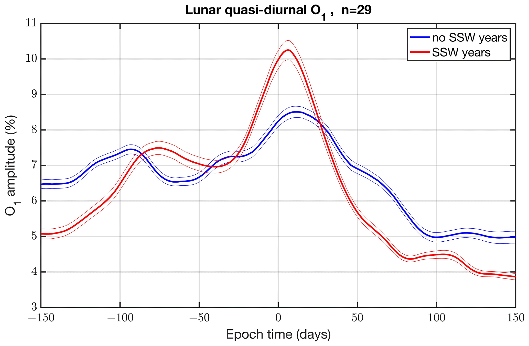
Figure 7 Composite of the relative amplitude of the quasi-diurnal lunar O₁ tide of NmF2 in Okinawa as a function of epoch time for the SSW years (red) and no-SSW years (blue). The thin lines denote the standard errors. In total, the composite consists of 29 SSW events from 1973 to 2022.

We compile a composite of the FFT spectrum in the SSW years and no-SSW years in order to get an overview of the spectral components of possible solar and lunar tides. The data segment spans from 5 weeks before the SSW event to 5 weeks after the SSW event. Figure 6 shows the result using a zoomed-in view which does not cover the peak in the solar diurnal variation S₁. The S₁ peak is at 96.4 % in the no-SSW years and at 95.4 % in the SSW years. The semidiurnal components of the sun (S₂) and the moon (M₂; period 12.42 h) are enhanced during the SSW years. In addition, we can see the quasi-diurnal lunar component (O₁; period 25.82 h), with 11.1 % in the SSW years and 8.8 % in the no-SSW years. However, there is a peak at the 25 h period in the no-SSW years, which is close to the lunar day (24.83 h). Possibly for the first time, we find a lunar terdiurnal component (MK₃; period 8.18 h), which is named the shallow-water terdiurnal tide. The MK₃ component reaches 5 % in the SSW years. It is evident that all lunar components in Fig. 6 have periods that align with those of ocean tides (Li, 2022). Due to the interannual variability in the tidal components, the standard error σ of the FFT spectra is often the same size as the enhancements during the SSW years. Figure 6 also shows a spectral peak at about 30 d, which is close to the synodic period of the moon cycle (29.53 d). At a frequency 0.5 cpd, we can see a significant peak in the 2 d oscillation during the no-SSW years, while the peak turns into a valley during the SSW years.

Finally, we wanted to study the time evolution of the amplification of the quasi-diurnal lunar O₁ tide. We derived a time series of the O₁ amplitude using moving FFT spectra with a window length of 10 weeks, following the same procedure as described above. Figure 7 shows an amplification of the O₁ tide just after the SSW onset at epoch time 0 (red curve indicating the SSW years).

2.1.1 Discussion

The attribution of ionospheric effects to individual major SSWs is a difficult task with respect to Okinawa, which is in the northern low-latitude ionosphere. The case study of the SSW on 6 January 2013 suggested that the semidiurnal cycle of NmF2 might be amplified after the SSW onset. Indeed, we find an increased peak in the semidiurnal amplitude on 16 January 2013, which coincides with the amplified semidiurnal pattern vertical ion drift and TEC above the magnetic equator from 15 to 19 January 2013 that was reported by Goncharenko et al. (2013). The plasma fountain in the equatorial ionosphere may slightly modulate the ionosphere above Okinawa, although Okinawa is located slightly north of the equatorial ionization anomaly (EIA). The result of an increased amplitude of the semidiurnal cycle of NmF2 in Okinawa was confirmed by a coincident amplitude increase observed at the nearby ionosonde station in Wuhan, China.

Since the ionospheric SSW effects are possibly smaller in Okinawa than at the magnetic equator, it makes sense to perform a composite analysis of 29 SSW events since 1972. The composite analysis describes the average behavior of the ionosphere before, during, and after SSW onsets. Moreover, we divided the observations into SSW years and no-SSW years and calculated the composites for both cases. This approach is powerful for critically assessing SSW effects despite high ionospheric variability caused by other sources, such as solar and geomagnetic variability or variability in atmospheric waves from below. The composite analysis showed that a peak in the semidiurnal cycle of NmF2 occurs at the epoch time 0 (SSW onset). This result is supported by the composite of the no-SSW years, which showed no peak at epoch time 0. This result is important since a peak might be attributed to the winter maximum of the amplitude of the semidiurnal cycle (Zolotukhina et al., 2011). Our data analysis clearly shows that the peak cannot be explained by the seasonal variation since the SSW-induced peak ionospheric amplitude does not occur in the no-SSW years. However, it is also noteworthy that the SSW effect is not so strong – the relative amplitude is 38.2 % in the SSW years and 32.9 % in the no-SSW years.

The long-term series of ionosonde observations are very valuable for studying the SSW effects of historical SSW events, and we found that the SSW of 31 December 1984 generated a relative amplitude of 162 % in the semidiurnal cycle of the relative NmF2 variations in Okinawa. In addition, we find that the amplitude increase in no-SSW years can also be quite strong, a factor to consider when analyzing the ionospheric effects of individual SSW events.

The most important finding of our study lies in the composites of the FFT spectra of the 29 SSW events. The solar (S₂) and lunar tidal components of NmF2 are increased during the SSW years compared to the no-SSW years. We find strong diurnal (O₁), semidiurnal (M₂), and terdiurnal (MK₃) components of the moon. The maximum of the O₁ amplitude occurs just after the SSW onset (Fig. 7). The periods of the lunar components correspond to those of ocean tides (Li, 2022) and also align well with the three periods of lunisolar variations in the atmosphere reported by Malin and Chapman (1970). In addition, the amplitudes are about 10 % for O₁ and M₂ and 5 % for MK₃ (Fig. 6). This is totally different from the results obtained for the Kokubunji ionosonde in Tokyo (not shown here), where we do not find significant lunar components. Past studies by Forbes and Zhang (2019) and Pedatella (2014) noted lunar diurnal and semidiurnal tides with an ionospheric electron density of up to 5 %. In the SSW years, we observe double this value in Okinawa. One possible explanation could involve strong non-migrating lunar tidal components which are excited by ocean tides at the ocean–atmosphere boundary. The strong lunar tides only occur in the winter season in Okinawa. Perhaps, especially in SSW winters, there are special vertical propagation conditions for solar and lunar tides. The breaking or dissipation of tides in the upper mesosphere and lower thermosphere induces a tidal signal in the neutral and ion temperatures at these heights, which is immediately transferred by heat conduction to the ionospheric F2 region. These tidal variations in the ion temperature induce tidal variations in the ionospheric plasma and the peak electron density (NmF2) (Zolotukhina et al., 2011).

It is interesting that the 2 d oscillation in NmF2 is strong in the no-SSW years, while it is missing in the SSW years (Fig. 6). This can be attributed to interactions of the tides with the quasi-2 d wave (QTDW) (Yue et al., 2016) or to different propagation conditions of the 2 d wave from below in the SSW years and no-SSW years. A composite shows a peak in the QTDW in NmF2 during the no-SSW years in winter, while the peak disappears in SSW winters (not shown in the present study). The synodic period of the moon (29.53 d) has strong peaks in both FFT spectra. Since the data segment was relatively short (10 weeks), a longer time interval is needed for a better distinction between the spectral peaks of the synodic period of the moon and the 27 d solar rotation cycle.

Vokhmyanin et al. (2023) reported that enhanced solar activity leads to a higher occurrence rate of SSWs. Indeed, the SSW years from 1973 to 2023 have an average F10.7 index of 122 sfu, while the no-SSW years have an average value of 112 sfu. This may explain why NmF2 in Okinawa was increased in the SSW years by 26 % compared to the no-SSW years (not shown in the present study). Further indications are that there were no SSWs from 1990 to 1997 and that a solar minimum occurred in 1994–1995. However, the flat composites of solar or geomagnetic activity in the SSW years cannot explain the peak in stratospheric temperature or the peak in the ionospheric semidiurnal amplitude (Fig. 4) at the SSW onset time. On the other hand, it is interesting to better understand why the mean state of the ionosphere is different in the SSW years compared to the no-SSW years; correlated changes in the ENSO and quasi-biennial oscillation (QBO) may also play a role (Vokhmyanin et al., 2023).

3 Conclusions

We find a clear SSW effect in the foF2 series for Okinawa (Fig. 3). In the composite of 29 SSW events, the amplitude of the semidiurnal cycle of foF2 shows a peak at the SSW onset time in the SSW years. This peak is certainly not due to seasonal effects since the peak disappears in the composite of the no-SSW years. To an extent, our analysis method is powerful for a critical assessment and attribution of SSW effects in the highly variable ionosphere. Composites of solar and geomagnetic activity showed no relevant variations at the SSW onset time, but the solar activity was generally higher in the SSW years than in the no-SSW years. The composite of the relative NmF2 variations also shows a significant peak in the semidiurnal amplitude at the SSW onset time in the SSW years (Fig. 4).

The evolution of the amplification of the semidiurnal amplitude of the relative NmF2 variations in winter is shown from 1972 to 2023 (Fig. 5). It is evident that the amplification of the semidiurnal amplitude can also occur during no-SSW years. Thus, the major SSWs cannot be the sole reason for a sudden amplification of the semidiurnal amplitude in the ionosphere above Okinawa. Other processes, such as minor sudden stratospheric warmings or variability in the mesospheric polar vortex, may play a role in the years without major SSWs.

The solar and lunar tidal components in Okinawa are slightly enhanced during the SSW years compared to the no-SSW years (Fig. 6). For the first time, we find a lunar terdiurnal component with a relative amplitude of about 5 % in the SSW years. The lunar diurnal and semidiurnal components have relative amplitudes of about 10 % in the SSW years. The periods of the lunar ionospheric tidal variations coincide with the periods of ocean tides and lunisolar variations in the atmosphere (Li, 2022; Malin and Chapman, 1970). Our study shows that the long-term series of foF2 and NmF2 from ionosondes are valuable for learning about the ionospheric effects of historical SSWs and for the study of lunar tides which are excited in the ocean–atmosphere system.