Interactions between trade wind clouds and local forcings over the Great Barrier Reef: a case study using convection-permitting simulations

Trade wind clouds are ubiquitous across the subtropical oceans, including the Great Barrier Reef (GBR), playing an important role in modulating the regional energy budget. These shallow clouds, however, are by their nature sensitive to perturbations in both their thermodynamic environment and microphysical background. In this study, we employ the Weather Research and Forecasting (WRF) model with a convection-permitting configuration at 1 km resolution to examine the sensitivity of the trade wind clouds to different local forcings over the GBR. A range of local forcings including coastal topography, sea surface temperature (SST), and local aerosol loading is examined.

This study shows a strong response of cloud fraction and accumulated precipitation to orographic forcing both over the mountains and upwind over the GBR. Orographic lifting, low-level convergence, and lower troposphere stability are found to be crucial in explaining the cloud and precipitation features over the coastal mountains downwind of the GBR. However, clouds over the upwind ocean are more strongly constrained by the trade wind inversion, whose properties are, in part, regulated by the coastal topography. On the scales considered in this study, the warm-cloud fraction and the ensuant precipitation over the GBR show only a small response to the local SST forcing, with this response being tied to the surface flux and lower troposphere stability. Cloud microphysical properties, including cloud droplet number concentration, liquid water path, and precipitation, are sensitive to the changes in atmospheric aerosol population over the GBR. While cloud fraction shows little responses, a slight deepening of the simulated clouds is evident over the upwind region in correspondence to the increased aerosol number concentration. A downwind effect of aerosol loading on simulated cloud and precipitation properties is further noted.

1 Introduction

Trade wind cumuli are ubiquitous across the subtropical oceans (Warren et al., 1988; Norris, 1998; Eastman et al., 2011; Boucher et al., 2013; Rauber et al., 2007), including the Great Barrier Reef (GBR) (Zhao et al., 2022). Despite their limited vertical and horizontal extent, these clouds play a fundamental role in maintaining the thermodynamic budget of the lower troposphere (Chen et al., 2000). These clouds reflect a significant fraction of incoming solar radiation and emit longwave radiation at relatively high temperature, and thus exert a net cooling effect on the earth atmosphere system (Mumby et al., 2001; Jones et al., 2017). Globally, these clouds help govern Earth's energy budget but are known to be a leading source of uncertainty in future climate projections (Boucher et al., 2013).

The GBR has become increasingly threatened by thermal coral bleaching events (CBEs) over the past decade (Hughes et al., 2017; Stuart-Smith et al., 2018). Recent research has also found that local-scale cloud cover helps regulate the ocean temperature along the GBR, with anomalies in the cloud fraction having been directly linked to thermal CBEs (Zhao et al., 2021; Leahy et al., 2013). However, while the large-scale circulation has a fundamental influence on shallow-cloud formation, these cloud systems by their nature are sensitive to perturbations in both their thermodynamic environment and microphysical background (Stevens and Brenguier, 2009; Rauber et al., 2007). It is therefore important to understand the sensitivity of these low clouds in response to different local forcings.

The GBR contains the world's largest complex collection of coral reefs. It has been hypothesized that the coral reef emissions of dimethyl sulfide (DMS) may be an important contributor to the regional atmospheric aerosol loading (Cropp et al., 2018). Any perturbation to the aerosol population could potentially affect the cloud properties and thus the radiative forcing (Lohmann and Feichter, 2005), for instance through a Twomey effect (Twomey, 1977). It has further been hypothesized that the aerosol loading can also affect the precipitation efficiency of these clouds, and thus their lifetime (Cropp et al., 2018; Fischer and Jones, 2012; Deschaseaux et al., 2016; Jones, 2015) through an Albrecht effect (Albrecht, 1989).

Over the GBR, a recent climatology study by Zhao et al. (2022) revealed little to no difference in low-level cloud properties between the open ocean (reef-free region) and the coral reef region using long-term satellite datasets. These results suggest that low clouds over the GBR do not show a measurable response to the reef-related microphysical perturbations, at least using spaceborne observations. However, subtle signals may be obscured or diminished when averaged over extensive periods in long-term climatological analyses. While a very small natural contribution to the cloud condensation nuclei (CCN) population from coral-derived DMS was noted over the GBR by either global (Fiddes et al., 2021) or regional-scale (Fiddes et al., 2022; Jackson et al., 2022) simulation studies, broader impacts of aerosol on cloud and precipitation processes over the GBR remain unquantified. For example, anthropogenic emissions are found to be important over the GBR in regard to modulating the influence from coral-reef-derived aerosol on local aerosol burdens. In addition, a higher temporal resolution analysis including the diurnal cycle of these low-level clouds may be critical in understanding their effect on the radiation budget (Fiddes et al., 2022; Fiddes, 2020). It is therefore appropriate to employ high-resolution convection-permitting modeling as an investigation tool to elucidate the full life cycle of these clouds, the development of the precipitation, and their response to any perturbations in the aerosol loading (Colle et al., 2005; Smith et al., 2015).

Variations in sea surface temperature (SST), from the shallow water area off the coast to the deeper open ocean and from low to high latitudes over the GBR, could also lead to differences in cloud properties, especially for boundary layer clouds (Crook, 1996). SST directly contributes to the thermodynamic conditions, which modulate the sensible and latent heat fluxes, and consequently cloud properties, such as cloud cover, cloud-top height, and cloud base (Bony et al., 2004). Significant positive SST anomalies are known to be a key driver of severe thermal coral bleaching periods across the GBR (Berkelmans et al., 2004; Hughes et al., 2017). These large SST anomalies, which could be prevalent for a few months and may spike during periods of weak winds (Filipiak et al., 2012; Gentemann et al., 2003; H. Zhang et al., 2016), are hence expected to produce a strong local forcing that could change the local thermodynamic conditions.

In addition to the aerosol and SST variations, clouds over the GBR can experience other local forcing mechanisms unique to this region. For example, orographic forcing could potentially be important when the southeasterly trade winds blow clouds across the Queensland coast and encounter the Great Dividing Range (Houze, 2012). The Wet Tropics of Queensland stretches along the northeastern coast of Australia for around 450 km roughly between 15–19° S (between the towns of Cairns and Townsville), where significant topography of ∼1000 m with a peak height of 1612 m at Mount Bartle Frere (Sumner and Bonell, 1986) is present. Pronounced precipitation enhancement over the windward slopes of the mountain barrier (Roe, 2005) is commonly observed. The mean annual accumulated rainfall over this large area is among the greatest in Australia (e.g., Bonell and Gilmour, 1980), with the Bellenden Ker Top station receiving over 8000 mm of annual precipitation (Herwitz, 1986) on average. Zhao et al. (2022) found significant orographic enhancement of low-level clouds over not only the Wet Tropics but also the upwind ocean extending partially over the GBR. It is therefore of interest to examine any upwind effect of orographic enhancement on shallow cloud and precipitation through high-resolution numerical simulations, where interactions of local variability associated with topography and coastal processes are better resolved.

In this paper, we undertake a case study using a series of simulations to explore the sensitivity of trade wind cumulus over the GBR to these different local forcings. In particular, we seek to address the following three scientific questions. (i) How does the topography of the Great Dividing Range affect the shallow clouds and precipitation over the Wet Tropics including the GBR? (ii) Is there any evidence of changes in cloud and precipitation properties in response to SST variations across the GBR? (iii) How do the shallow-cloud and precipitation properties respond to enhanced local aerosol loading, both over the GBR and downwind over the coast of Queensland? Unlike the study of Fiddes et al. (2021, 2022), this study does not aim to test the effects of DMS directly. Rather, it focuses on understanding how strongly, if at all, cloud and precipitation properties respond to changes in the atmospheric aerosol number concentration related to surface emissions. This analysis is also relevant to understanding the integrated effects of potential weather and climate interventions, such as marine cloud brightening, in the heat-sensitive environment of the GBR and its adjacent communities.

To address these questions, a range of sensitivity experiments is conducted using convection-permitting numerical simulations. This paper is divided into six sections as follows: Sect. 2 gives a brief description of the background climate and the meteorological conditions of the region, Sect. 3 details the data and methods used in this study. The main results and discussion are presented in Sects. 4 and 5. Section 6 summarizes the results and provides prospects for future research.

2 The 29 April 2016 case study

The GBR is characterized by a warmer than average monthly sea surface temperature during April 2016 when a thermal coral bleaching event was reported (Zhao et al., 2021). An SST anomaly of over 1 °C is identified across much of the GBR (Fig. S1 in the Supplement), with this SST anomaly being likely to affect the cloud properties, especially low-level clouds, through marine atmospheric boundary layer (MABL) processes (Qu et al., 2015; Takahashi et al., 2021). This selected case is characterized by local trade wind cumulus over the Wet Tropics and associated with orographic precipitation on 29 April 2016. This event is also chosen due to the absence of high cloud cover across the Wet Tropics, which is often linked to deeper convection governed by large-scale climate modes such as El Niño–Southern Oscillation (ENSO) and Madden–Julian Oscillation (MJO), as well as the Australian monsoon or tropical cyclones (Tian et al., 2006; Yuan and Houze, 2013; Eleftheratos et al., 2011; Wu et al., 2012). Note that there is a weak El Niño phase of ENSO during the case study period. Further, the MJO is weak, with the real-time multivariate MJO index (Wheeler and Hendon, 2004) being less than 1, and no tropical cyclones are recorded across northeastern Queensland and the GBR.

The mean sea level pressure (MSLP) analysis at 12:00 UTC on 28 and 29 April 2016 (Fig. 1a and b) reveals a Tasman High maintaining the southeasterly trade winds along the northeastern coast of Queensland during the case period. Originating in southwestern Australia on 22 April, this high-pressure system gradually progressed eastward (not shown). By 26 April, it was positioned over southeastern Australia, consequentially producing a high ridge along the northeastern coast of Queensland during the following 4 d. As shown in the Himawari-8 true-color images (Fig. 1c) at 00:00 UTC 28 April 2016, northeastern Queensland mostly has a clear sky with patches of low-level clouds (stratocumulus, cumulus, and stratus, as shown in Fig. 1e) extending southwest from the coast in the Wet Tropics. Satellite observations at 05:00 UTC on 29 April 2016 (Fig. 1f) reveal a well-developed cloud system consisting of stratocumulus, altocumulus, and altostratus. Orographic precipitation associated with trade wind cumuli is captured by land-based rain gauges at several weather stations (Fig. 2) on 29 April. The heaviest precipitation was recorded over the eastern slopes and mountain peaks, which is expected under the influence of upslope lifting under the prevailing southeasterly wind regime. From 06:00 UTC on 30 April, the cloud system over the Wet Tropics started dissipating, as observed by satellite images (not shown).

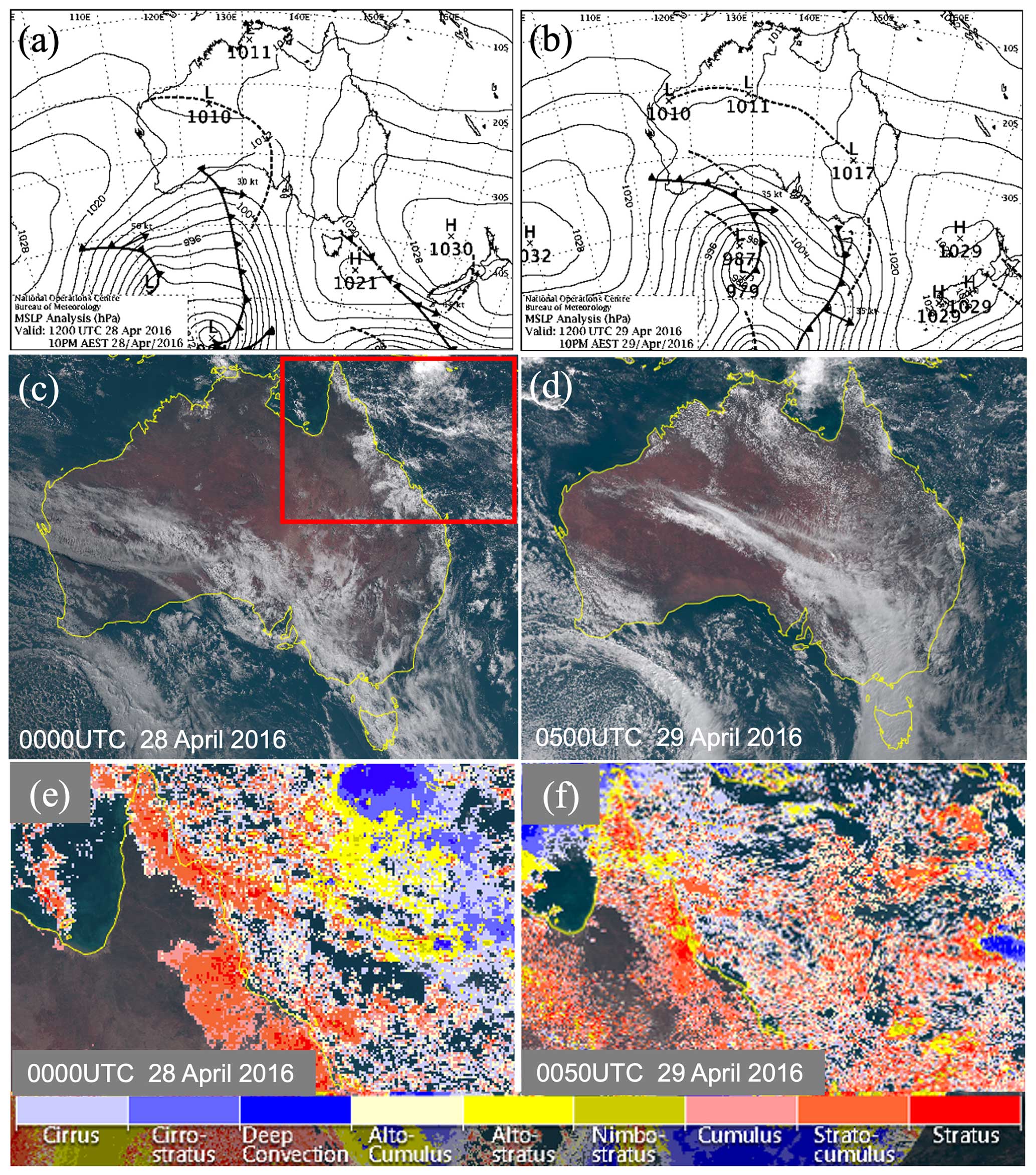
Figure 1 Mean sea level pressure (MSLP) analyses for the April 2016 case at (a) 12:00 UTC on 28 April and (b) 12:00 UTC on 29 April 2016. Himawari-8 true-color imagery for (c) 00:00 UTC on 28 April and (d) 05:00 UTC on 29 April 2016. Himawari-8 cloud type classification for (e) 00:00 UTC on 28 April and (f) 05:00 UTC on 29 April 2016 for the domain shown by the red rectangle in (c). Cloud types as listed on the color bar for (e, f) are cirrus, cirrostratus, deep convection, altocumulus, altostratus, nimbostratus, cumulus, stratocumulus, and stratus. The images used in panels (a) and (b) are provided by the Australian Bureau of Meteorology. The images used in panels (c)–(f) are supplied by the P-Tree System, Japan Aerospace Exploration Agency (JAXA).

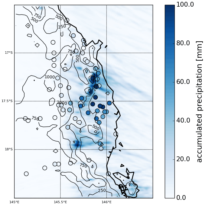
Figure 2 The 48 h accumulated simulated precipitation amounts from 1 km resolution with CTRL from 23:00 UTC on 27 April to 23:00 UTC on 29 April 2016 overlaid with the precipitation observed by rain gauges shown as filled circles using the same color scale. Black contours indicate the topography map from 250 to 1500 m in 250 m intervals.

3 Data and methodology

3.1 Model configuration

The Weather Research and Forecasting (WRF, version 4.2; Skamarock et al., 2019) model is used to simulate the interactions between trade wind cumulus and local forcings. In this study, the model is configured with unevenly distributed 65 levels in the vertical (Fig. S2), allowing for 30 levels in the lowest 3 km where most of the trade cumulus clouds reside. Three nested domains with horizontal grid spacing of 9, 3, and 1 km are utilized (Fig. 3a). The innermost domain (d03) is set up with 562×457 grid points covering most of the significant topography over the Wet Tropics (Fig. 3b), extending over the GBR. The model uses the fifth-generation atmospheric reanalysis (hourly, 0.25°×0.25° grid, 37 set pressure levels and surface level) from the European Centre for Medium-Range Weather Forecasts (ERA5 reanalysis, Hersbach et al., 2018, 2020), for initial and lateral boundary conditions, as part of the standard WRF pre-processing system (WPS). Following initialization, the model is allowed to run freely with no nudging applied, which enables the meteorology to fully develop throughout the simulation. The control (CTRL) simulation is initialized at 12:00 UTC on 27 April 2016 and run for 3 d (i.e., 72 h), with the first 12 h being used as the spin-up time. It is worth noting that sensitivity to different spin-up times (e.g., 12, 18, and 24 h) has been tested as the optimal spin-up time configuration may vary across different case studies, reflecting the unique atmospheric conditions and dynamics inherent to each scenario. The results indicate that the simulation with a shorter spin-up time (12 h) produces a better agreement with observations for this case (not shown).

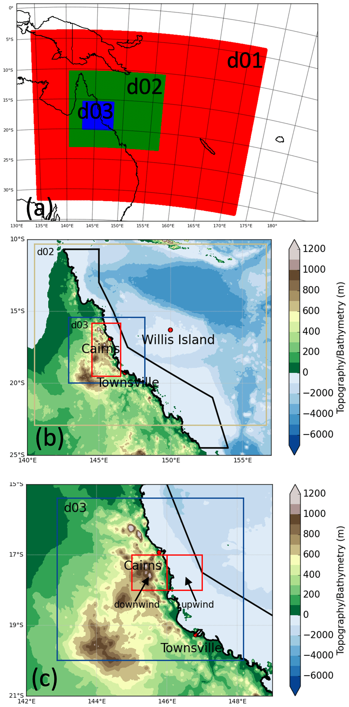
Figure 3 (a) The WRF three nested domains shown by different color boxes used in this study. (b) Zoomed-in topographic–bathymetric map of the two inner domains (shown by colored rectangles) with the locations of two sounding stations (Townsville and Willis Island). The solid red rectangle points out the location of the Wet Tropics. Black lines indicate the GBR general reference map. (c) The 1°×1° downwind and upwind sub-domains shown by red rectangles.

Table 1 A list of configuration settings for numerical study.

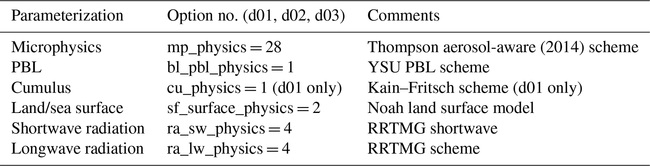
The history intervals of prediction outputs are set to be 6 h for d01, 3 h for d02, and 1 h for d03. Simulations are performed with the Yonsei University (YSU, Hong et al., 2006, first-order nonlocal) planetary boundary layer (PBL) scheme, “Noah” land surface model (Chen and Dudhia, 2001), and the RRTMG (Mlawer et al., 1997) scheme for shortwave and longwave radiation, respectively. The same schemes are used for each domain, with the exception of the cumulus scheme. The Kain–Fritsch (Janjić, 2000) cumulus parameterization is used only for the coarsest domain (d01) to represent sub-grid convection. For the microphysical parameterization, the Thompson aerosol-aware microphysics scheme (Thompson and Eidhammer, 2014), a bulk scheme that treats five separate water species, cloud water, cloud ice, rain, snow, and a hybrid graupel–hail category, is used. This scheme utilizes double-moment prediction (mass and concentration) of cloud water, cloud ice, and rain mixed with single-moment prediction (mass only) of snow and graupel. Updated from the previous version (Thompson et al., 2008), this version of microphysics scheme incorporates the activation of aerosols as cloud condensation (CCN) and ice nuclei (IN), and it therefore explicitly predicts the number concentration of two aerosol variables. Rather than assuming all model horizontal grid points have the same vertical profiles of CCN and IN aerosols, this study uses an auxiliary aerosol climatology as the aerosol background condition placed into WRF model for every grid point, regardless of cloudiness. The aerosol input data are derived from multiyear (2001–2007) global model simulations (Colarco et al., 2010) in which particles and their precursors are emitted by natural and anthropogenic sources. Multiple species of aerosols, including sulfates, sea salts, organic carbon, dust, and black carbon, are explicitly modeled with multiple size bins by the Goddard Chemistry Aerosol Radiation and Transport model with 0.5° longitude by 1.25° latitude spacing. The microphysical scheme then transforms these data into simplified aerosol treatment by accumulating dust mass larger than 0.5 µm into the IN (ice-friendly) mode and combining all other species besides black carbon as an internally mixed CCN (water-friendly) mode. To get the final number concentrations from mass mixing ratio data, it is assumed that lognormal distributions are used, with characteristic diameters and geometric standard deviations taken from Chin et al. (2002). Samples of the climatological aerosol dataset can be found in Thompson and Eidhammer (2014, Fig. 1). Note that black carbon is ignored for this version but might be incorporated into future versions (Thompson and Eidhammer, 2014). However, it is not expected that the absence of black carbon aerosol will have a significant effect for pristine maritime trade cumulus clouds. Rather than considering multiple aerosol categories, the Thompson aerosol-aware microphysics scheme simply refers to the hygroscopic aerosol (a combination of sulfates, sea salts, and organic carbon) as a “water-friendly” aerosol and the non-hygroscopic ice-nucleating aerosol (primarily considered to be dust) as “ice friendly”. The activation of aerosols as CCN and IN is determined by a lookup table that employs the simulated temperature, vertical velocity, number of available aerosols, and hygroscopicity parameter applied in Köhler activation theory. The activation of aerosols as droplets is performed at cloud base and anywhere inside a cloud where the lookup table value is greater than the existing droplet number concentration (Thompson and Eidhammer, 2014). Note that the aerosols used by the microphysics scheme to activate water droplets and ice crystals do not scatter or absorb radiation directly. The aerosol's scattering–absorption–emission of direct radiation is only considered within the RRTMG radiation scheme by the typical background amounts of gases and aerosols in this study (Thompson and Eidhammer, 2014). The Thompson aerosol-aware scheme has been shown in previous studies to have promising skill in representing both supercooled and warm liquid conditions of grid-scale clouds (Weston et al., 2022; Wilkinson et al., 2013).

An overview of the parameterization schemes used in the CTRL simulation is provided in Table 1. It is worth noting that other configurations with different microphysics, boundary layer, and cumulus schemes have also been tested, and the simulation with the configuration listed in Table 1 is found to be most skillful when evaluated against observations. This configuration is therefore used as a CTRL run, and the same configuration settings are applied to all sensitivity experiments.

3.2 Sensitivity experiments

Five sensitivity experiments are undertaken to examine the impacts of various local forcings, as detailed below.

In the topography experiment, the orography above 300 m is reduced by 75 % (Fig. S3), named “Topo300”, as similarly done in Flesch and Reuter (2012) and Sarmadi et al. (2019). A threshold of 300 m is chosen because it is approximately the mean altitude of the Wet Tropics region, and it hence represents the background geography. A 75 % reduction is used in order to preserve some of the topographic features and to avoid drastic changes of topography that may induce dramatic changes in the larger-scale circulations. We note that a 500 m threshold is also tested and yielded similar results (not shown).

For the local SST forcing, two sensitivity simulations have been conducted in which the monthly mean climatological SST condition for April (namely “SST-climatology”, Fig. S1) and spatially uniformed 1 °C cooler than real SST condition (namely “SST-cooler”) are used to initialize the simulation. The monthly SST climatology applied in the control simulation is derived from ERA5 for the period of 1998–2018. This climatology integrates SST data from HadISST2 (before September 2007) and OSTIA (September 2007 onwards) datasets. It is important to note that, unlike the SST alteration in the SST-cooler experiment, part of the ocean area in the SST-climatology experiment is warmer than the actual SST (Fig. S1). Nevertheless, the sea surface temperature over the majority of the GBR is reduced in the SST-climatology experiment. The selection of a 1 °C perturbation is based on the findings presented in Zhao et al. (2021), where a typical 1 °C positive SST anomaly is noted during the coral bleaching season over the GBR. SST modifications are applied to the whole ocean area for all three domains. It should be noted that, as with CTRL, the SST conditions are fixed through the 3 d simulations.

Finally, the climatological surface water-friendly aerosol (WFA) emissions (kg⁻¹ s⁻¹) over the GBR (see general reference map in Fig. 3b) is increased by factors of 2 and 5 to test the sensitivity of warm cloud and precipitation to the aerosol loading to emulate a scenario of enhanced aerosol population associated with coral reef emissions (named “Aerosol2” and “Aerosol5”, respectively, Fig. S4).

Table 2 summarizes the details of these sensitivity experiments.

Table 2 Detailed information of numerical experiments conducted in this study.

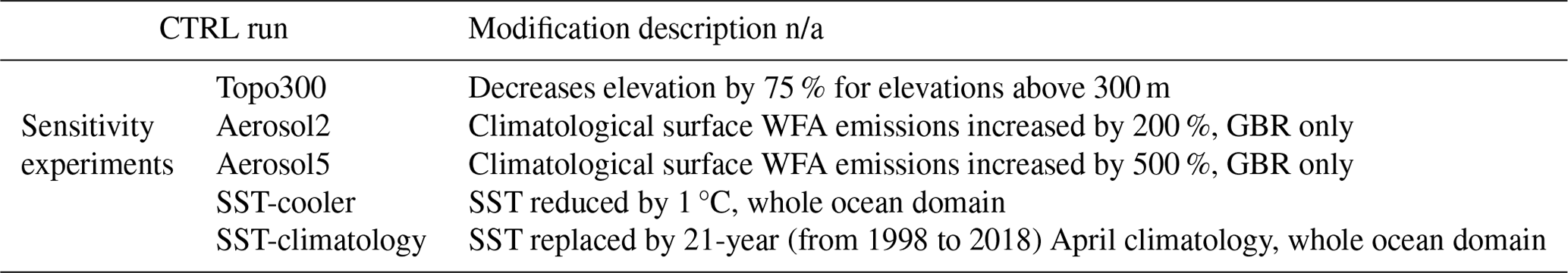
The notation n/a stands for not applicable.

3.3 Observational data

Several observational datasets and reanalysis are used to evaluate the simulation across a range of spatial–temporal scales. In this study, sounding data at 00:00 and 12:00 UTC during the simulation period are obtained from the University of Wyoming upper-air sounding database for two selected radiosonde stations (Townsville, code: 94294; Willis Island, code: 94299). To evaluate the large-scale meteorological background conditions in the simulation, hourly mean sea level pressure (MSLP) and wind field at 10 m are also obtained from ERA5 reanalysis with a resolution of 0.25° for the case period (Hersbach et al., 2020). Channel 13 brightness temperatures from the Himawari-8 satellite dataset (Bureau of Meteorology, 2021) and daily rainfall datasets from continuous weather stations are obtained from the Australian Bureau of Meteorology for the case study period. A total of 60 stations are selected, and their spatial distribution is shown in Fig. 6. It should be noted that some of thermodynamic observations (e.g., radiosonde soundings and wind observations) are being assimilated into the reanalysis; however, observations of cloud and precipitation are not. It is expected that the initial hours will exhibit strong agreement of thermodynamic variables with the ERA5 dataset, but over the course of the 36 h the simulations will be sensitive to the parameterizations and settings selected. Therefore, the evaluation of model output is designed to examine the middle and last few hours of the simulation (Figs. 4 and 5) against both ERA5 thermodynamics and independent cloud and precipitation observations (e.g., Himawari and weather station, Figs. 2 and 6).

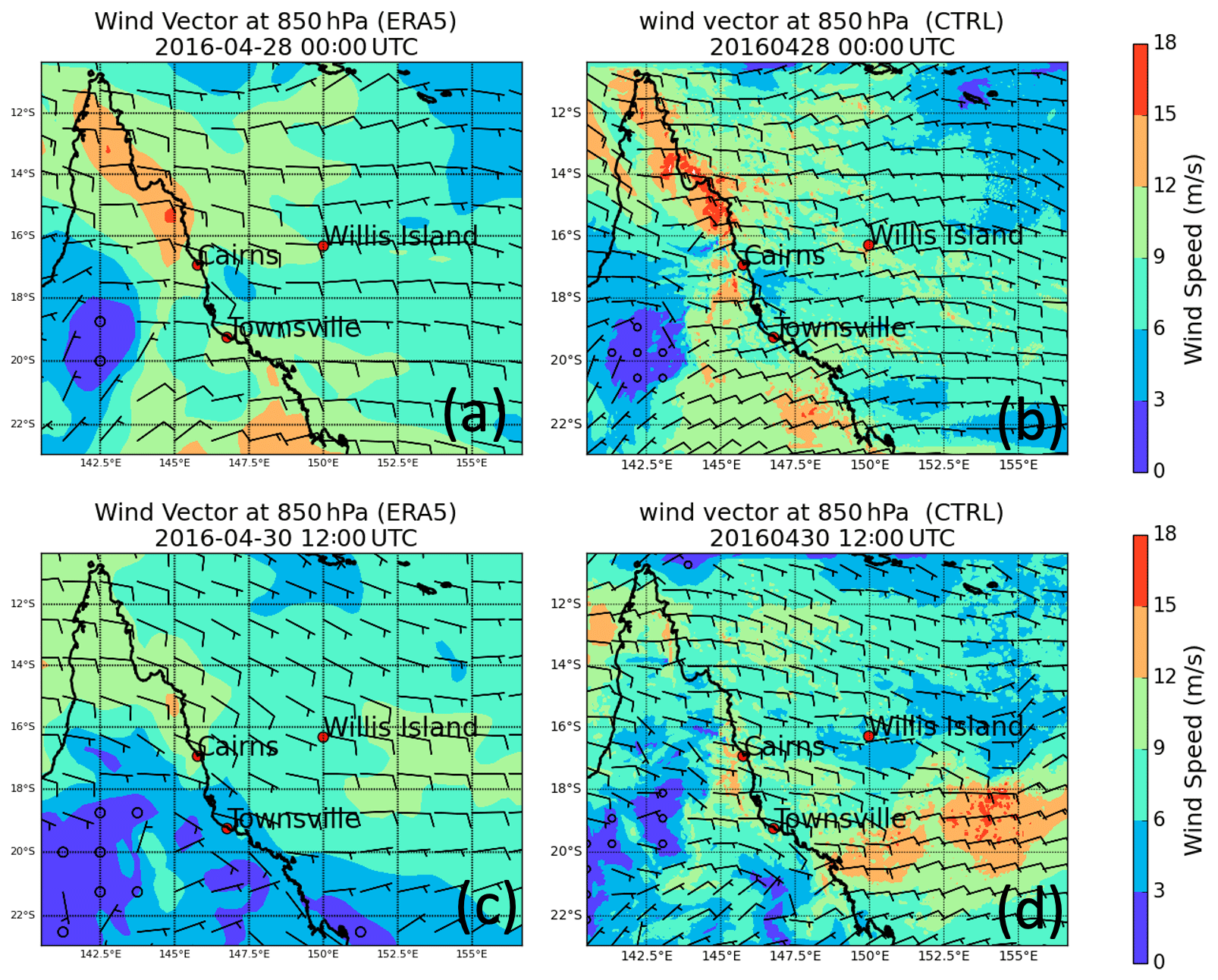
Figure 4 (a) Wind vector distribution at 850 hPa from ERA5 and (b) WRF simulations from the CTRL run at 00:00 UTC on 28 April 2016. Panels (c) and  (d) are the same as (a) and (b) but for 12:00 UTC on 30 April 2016. Note that same color scales are applied in all panels.

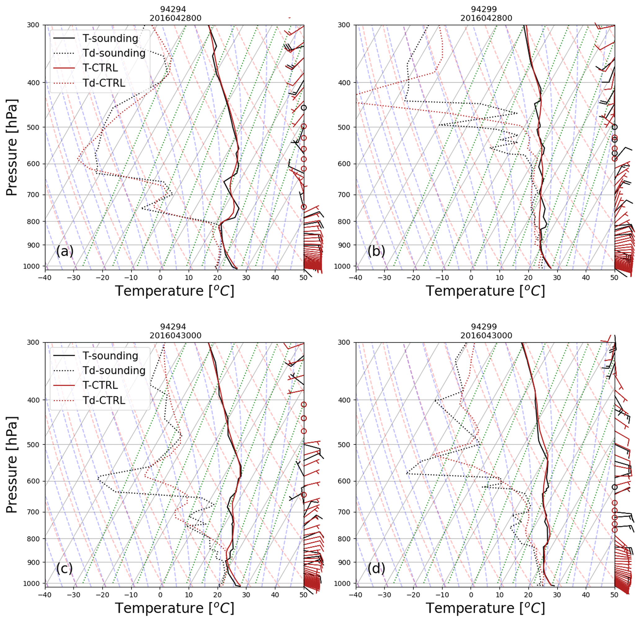
Figure 5 Comparison of the observed upper-air soundings (black lines) from (a) Townsville and (b) Willis Island alongside 3 km WRF simulations (red lines) from the nearest grid point to two stations on 28 April 2016 at 00:00 UTC. Panels (c) and  (d) are the same as (a) and (b) but for 00:00 UTC on 30 April 2016. Solid lines are for temperatures, and dotted lines represent dew point temperature.

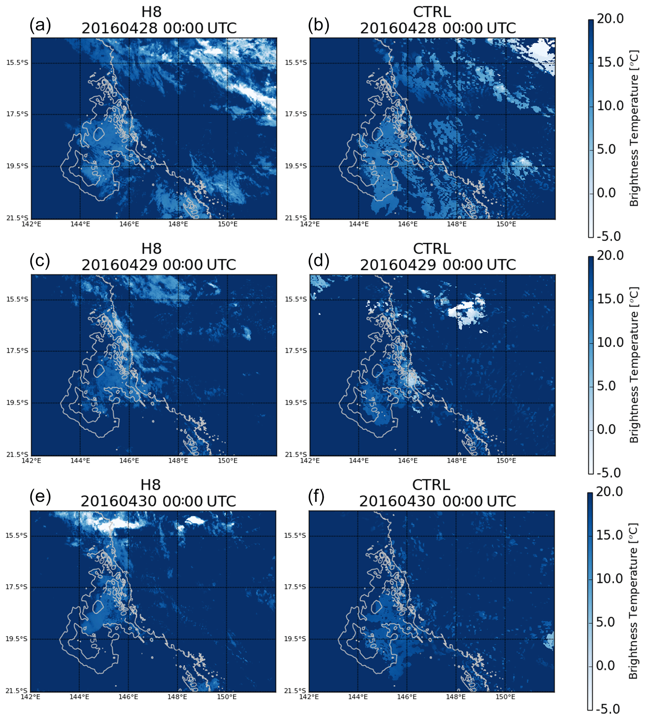
Figure 6 (a, c, e) Brightness temperatures of band 13 (10.4 µm) derived from Himawari-8 satellite observations at 00:00 UTC on 28, 29, and 30 April 2016. (b, d, f) Simulated brightness temperatures from CTRL at 3 km resolution at 00:00 UTC on 28, 29, and 30 April 2016. Note that same color scales applied in all panels. Grey lines denote the coastline and topography map from 500 to 1500 m with 250 m intervals.

3.4 Identifying the trade wind inversion

The trade wind inversion (TWI), which results from the interaction of large-scale subsiding air from the upper troposphere and rising air from lower levels that is driven by convection, plays an important role in defining cloud structure and vertical development (Riehl, 1979; Albrecht, 1984). Under a trade wind regime, the top of a cloud layer typically marks the base of the inversion.

In this study, we use the same criteria identified in Murphy (2017) to examine the TWI characteristics and its interaction with clouds. Four variables are used: (1) pressure, (2) height, (3) dry bulb temperature, and (4) relative humidity. The criteria used are as follows.

• a.

  The TWI is restricted to the 850–600 hPa layer and environmental temperatures greater than 273 K.

• b.

  The base of the TWI is defined where the temperature begins to increase, and relative humidity decreases with height.

• c.

  The top of the TWI is defined by a vertical temperature decrease with height.

• d.

  When multiple inversions are detected, the layer with the greatest relative humidity decrease is selected as the TWI.

Two properties, in addition to the inversion base height, describing the TWI are defined also following the method described in Murphy (2017). The inversion thickness (km) is the difference in height between the base and top of the inversion, while the inversion strength or magnitude (K) is the temperature increase across the inversion. It should be noted that grid points with no TWI identified (around 19 % of total samples) are excluded from the TWI analysis.

4 Control simulation

In this section, the simulated synoptic and the surface features are first evaluated by comparing the results of the control simulation with observations. It is found that the control simulation skillfully simulated the evolution of the large-scale synoptic patterns of the MSLP in terms of both the progression and the magnitude of the surface pressure system (not shown). Simulated wind conditions at 850 hPa at 00:00 UTC on 28 April (the first hour after spin-up time) are compared with ERA5 reanalysis, and the 3 km WRF simulated pattern and magnitude of the wind field are found to be generally in good agreement with the reanalysis (Fig. 4a and b). It should be noted that this is largely expected as the simulations are initialized with ERA5 reanalysis in this study. However, a good agreement is also found towards the end of the simulation (12:00 UTC on 30 April), suggesting that the simulation in this study is doing a good job regarding representation of the synoptic condition. As shown in Fig. 4c and d, both wind speed and direction agree reasonably well with the reanalysis, though a disagreement in the wind speed is noted in the southern part of the ocean. Figure 5 shows the observed soundings (black) from the two available sounding stations (Willis Island and Townsville) within the domain and the simulated atmospheric profile (red) at the nearest grid point in the 3 km domain at 00:00 UTC on 28 and 30 April. The simulated soundings at the two sites both have good agreement with observations at the beginning and the last day of the simulation, with both wind speed and direction well captured throughout the profile. The simulation accurately predicts the cloud base height (around 850 m) and surface temperature at the two sites, and it is worth noting that the wind inversion at 800 hPa at Townsville station is well captured throughout the simulation (Fig. 5).

Figure 5 compares the observed and simulated brightness temperature throughout the simulation period. Note that the simulated brightness temperature is simply calculated assuming an emissivity of 1 for all surfaces and an effective cloud optical depth of 1. It is used for a qualitative evaluation of the simulated cloud field only. Overall, the cloud field is reasonably well simulated in terms of the location and timing when compared against the Himawari-8 observation. Although the chaotic nature of shallow cumulus cloud means that details are not fully aligned, the major cumulus cloud features over the Wet Tropics throughout the 3 d simulation period have been well captured.

Figure 2 shows the 48 h accumulated precipitation from the 1 km WRF simulation, overlaid with the observed rainfall shown as filled circles using the same color scale. The orographic signature (see Fig. 3b and black contours in Fig. 6), as shown in the correlation between the accumulated precipitation amounts and topography, is evident in both the observed and simulated precipitation. The overall distribution of the simulated accumulated precipitation shows a good agreement with the rain gauge observations, with the majority of the precipitation produced over the windward side of the topography. Although a bias is noted in the location of the peak precipitation, with the simulated precipitation indicating a northward shift relative to the observation, the simulated accumulated precipitation amounts agree reasonably well with the rain gauge observations. This shows the model has acceptable skill in predicting precipitation patterns and magnitude, despite some spatial discrepancies.

5 Sensitivity analysis

5.1 Orographic effects

To explore any upwind effect of the orography over the Wet Tropics, two 1°×1° sub-domains are selected, with one covering the primary orographic area (hereafter downwind sub-domain, Fig. 3c) where the major precipitation occurs (see Figs. 2 and 9a) and another over the upwind water area (hereafter, upwind sub-domain, Fig. 3d). The simulated cloud fraction (CF) has been analyzed over these two sub-domains, respectively. Note that in the WRF output CF for each grid point is given by either 1 or 0 to indicate either cloudy or cloud-free pixel, respectively. In this study, CF of the target domain (e.g., 1°×1° upwind and downwind sub-domains) is defined as the proportion of total grid points in the domain that are classified as cloudy grids for each model level. For each model level from 0.5 to 6 km, the CF is calculated for each hour. Figures 7 and 8 show the two-dimensional probability density function (PDF) distribution of the CF across the domains for the 60 h of simulation. To generate the PDF, 100 bins are applied to both CF and altitude. The probability density for each grid point is then calculated based on CF samples at model levels from 60 simulations hours. The uppermost level of this analysis is set to 6 km as most of the clouds are observed to be at low to mid level during the simulation period. As shown in Figs. 7a and 8a, the simulated CF over these sub-domains from CTRL is between 0.5 and 2.5 km (i.e., boundary layer clouds and trade wind cumuli). Note that the boundary layer height over the Wet Tropics is around 950 m in the CTRL run (not shown) and that the trade wind inversion base is at around 2 km (see Fig. 10a).

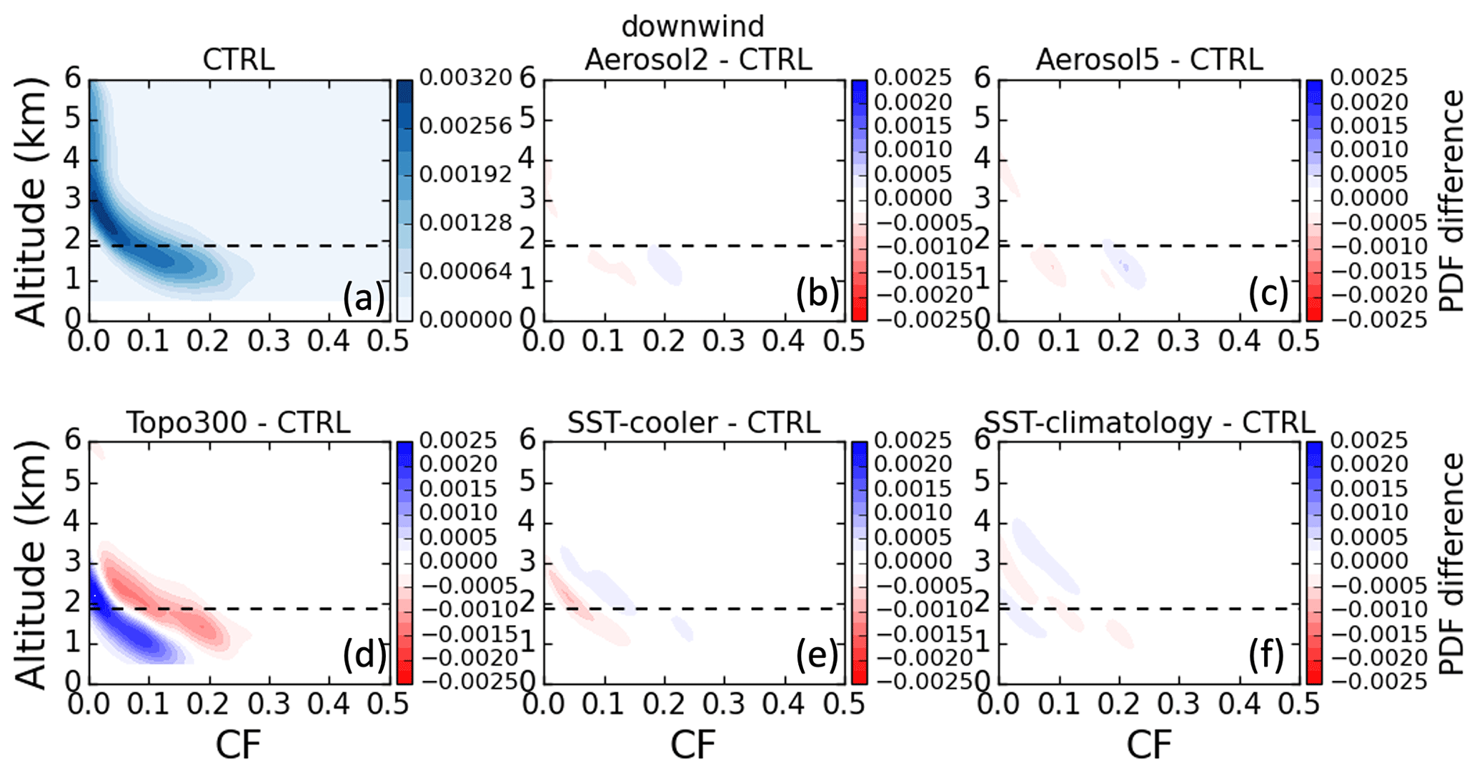
Figure 7 (a) Vertical PDF distribution of 1 km resolution simulated cloud fraction over the downwind mountain area (shown by the red square in Fig. 3c) from CTRL-run. (b–f) Difference plots between the CTRL run and Aerosol2, Aerosol5, Topo300, SST-cooler, and SST-climatology. The analysis is for 60 h simulation time after the spin-up from 00:00 UTC on 28 April to 12:00 UTC on 30 April 2016. Note that dashed lines indicate the average base height of TWI over the downwind sub-domain.

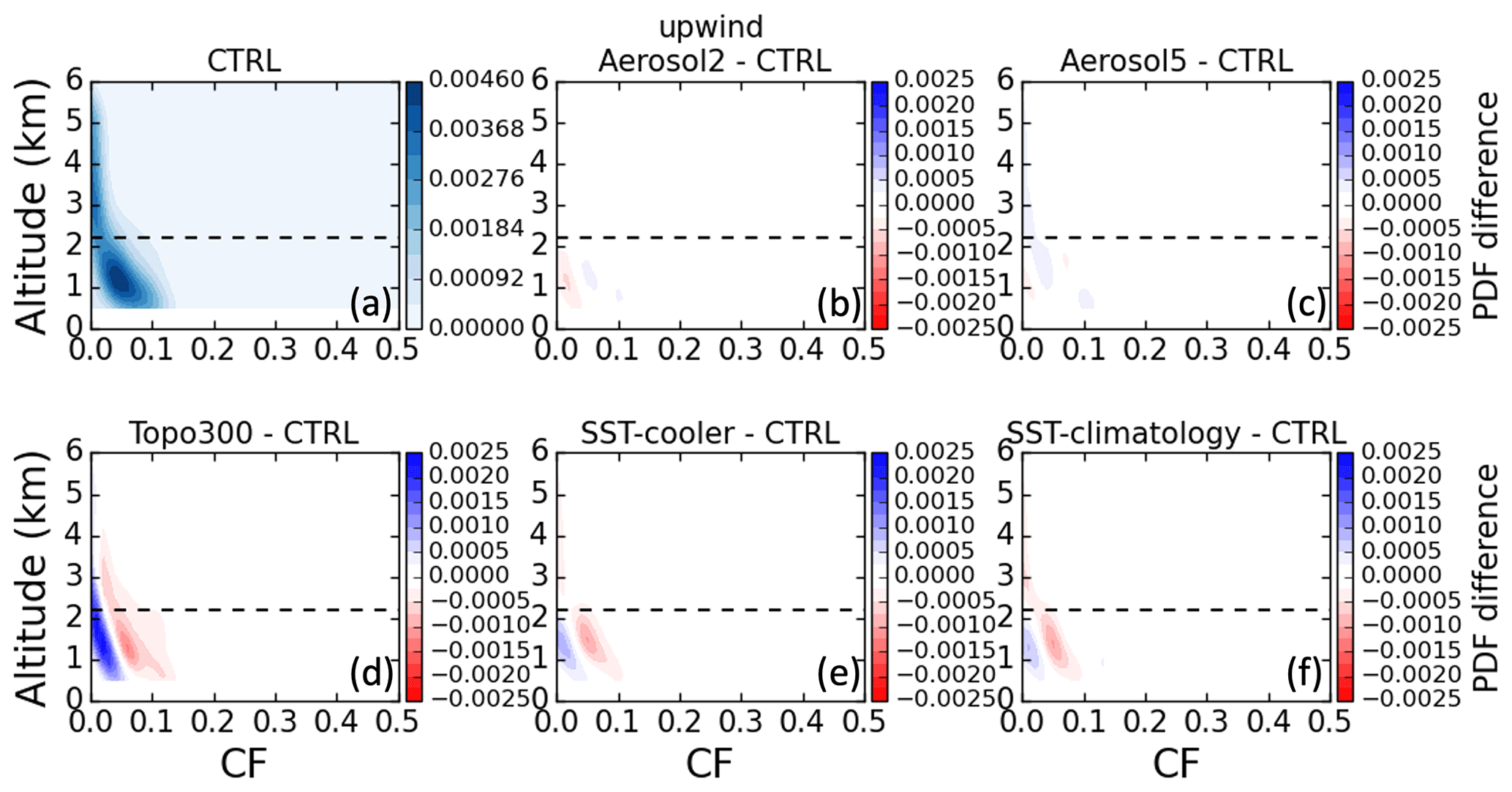
Figure 8 The same as Fig. 7 but for the upwind water area (shown by the red square in Fig. 3d).

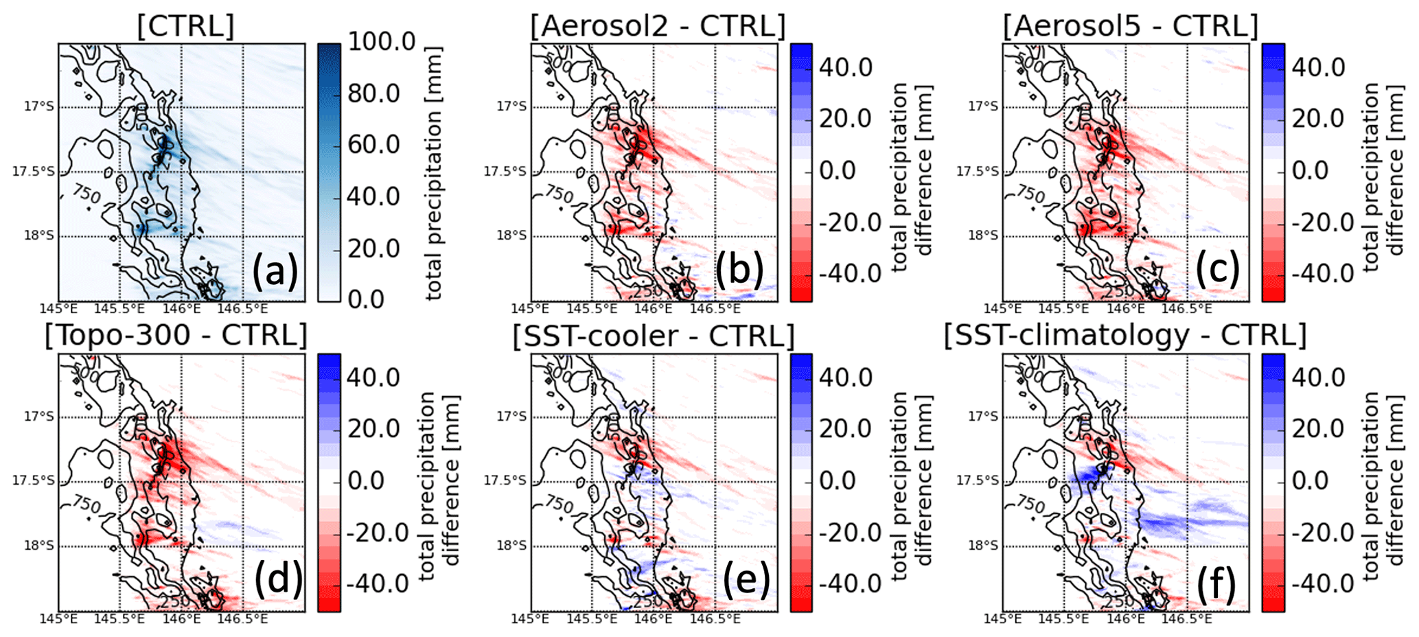
Figure 9 (a) Accumulated precipitation for the time period of 00:00 UTC on 28 April to 12:00 UTC on 30 April 2016 from 1 km resolution with CTRL-run. (b–f) Difference plots of accumulated precipitation between CTRL-run and Aerosol2, Aerosol-5, Topo300, SST-cooler, and SST-climatology. Black contours indicate the topography map from 250 to 1500 m in 250 m intervals.

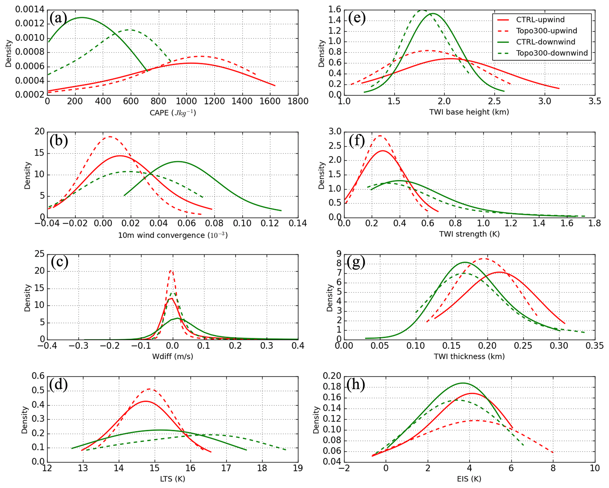
Figure 10 PDF distribution of the (a) CAPE, (b) low-level wind convergence, (c) W_diff, (d) LTS, (e) trade inversion base height, (f) inversion strength, (g) inversion thickness, and (h) EIS over the upwind (red lines) and downwind (green lines) area, separately. The analysis covers the whole 60 h simulation period after the spin-up time. Solid lines represent results from CTRL, and dashed lines are for Topo300 sensitivity experiment.

Comparing the simulated CF distribution between Topo300 and CTRL runs over the orographic area (Fig. 7d), there appears to be a noticeable decrease in cloud cover in the Topo300. The most pronounced reduction (∼78 %) is evident at lower altitudes, specifically below 2 km. Cloud-top height is generally reduced in Topo300, with a greater number of simulation hours in Topo300 indicating a CF near zero above 2 km. This same feature is also seen over the upwind coral reef area (Fig. 8d), though the magnitude of the CF is relatively small (∼40 %) compared to the mountain area. Larger differences in CF are, once again, found at lower altitudes (below 2 km). It is interesting to note that the orographic enhancement of the low-level cloud fraction, extending to the eastern water area, potentially provides a sheltered area for the coral reefs, protecting them from severe bleaching through reducing the solar radiation heating (examples of cloud fields are shown in Fig. S5). This result is consistent with the observational analysis presented by Zhao et al. (2022), which highlighted a notable increase in the frequency of low-level clouds associated with orographic enhancement in the Wet Tropics.

Figure 9 shows the map of accumulated precipitation over the innermost domain from 1 km WRF simulations from the CTRL run, and the difference between the CTRL run and sensitivity studies, respectively. The accumulation period is the 60 h simulation time after the spin-up (i.e., from 00:00 UTC 28 April to 12:00 UTC 30 April 2016). As shown in Fig. 9d, a strong reduction in precipitation (∼44 %) over the topography is evident when the topography is modified, particularly over the windward slopes. Over 40 mm difference in the accumulated precipitation is noted at the points of highest precipitation grids between the Topo300 and CTRL simulations, highlighting the major role of terrain in the development of precipitation. In addition to the mountain area, this precipitation reduction has also been seen over the upwind region, extending to the GBR. A slight increase in the accumulated precipitation is noted in the southern part of the upwind domain, indicating the chaotic nature of cloud and precipitation in weakly forced locations.

The local cloud and precipitation differences shown in Figs. 7d, 8d, and 9d can be elucidated through the examination of convection-related variables, including convective available potential energy (CAPE), 10 m wind convergence (calculated as $(-\mathrm{1})\times (\partial u/\partial x+\partial v/\partial y$), Schneider et al., 2018) and velocity difference (w_diff) between the maximum vertical velocity below the level of free convection (LFC) and the required updraft velocity to overcome convective inhibition (CIN), calculated as $\sqrt{\mathrm{2}\times \mathrm{CIN}}$ (Trier, 2003). Positive values of w_diff indicate that air parcels can reach their respective LFC, release CAPE, and initiate convection. In addition, simulated trade wind inversion (TWI) properties have been analyzed, including its base height, thickness, and strength. This analysis is important because trade wind cumuli are constrained by the TWI, particularly over the oceanic regions. It is also perhaps more difficult to directly link changes in cloud and precipitation process over the upwind domain to the direct mountain-induced lifting and low-level wind convergence. Additionally, the lower troposphere stability (LTS) and estimated inversion strength (EIS) have been examined, which are good indicators of the changes in low-level cloud (Wood and Bretherton, 2006). LTS is defined as the potential temperature difference between a nominal location in the free troposphere (typically 700 hPa) and the surface. EIS is further developed to obtain a more precise estimate of the strength of the boundary layer inversion by removing the variability of the free tropospheric thermodynamic structure (Wood and Bretherton, 2006), which is defined as $\mathrm{LTS}-{\mathrm{\Gamma }}_{\mathrm{m}}^{\mathrm{850}}(z_{\mathrm{700}}-\mathrm{LCL})$, where ${\mathrm{\Gamma }}_{\mathrm{m}}^{\mathrm{850}}$ is the moist adiabatic potential temperature lapse rate, z₇₀₀ is the altitude of the 700 hPa pressure level, and LCL is the lifting condensation level computed using the expression $\mathrm{LCL}=\mathrm{125}(T--\mathrm{Td})$, which is based on the temperature (T) and dew point temperature (Td) at the surface (Lawrence, 2005). Note that all of these variables are calculated for each grid point at each hour.

As seen from Fig. 10a, a notable increase in CAPE is seen in the Topo300 over the downwind area, whereas only small increases are found upwind. This change in CAPE is clearly explained by the change in orography. The atmosphere deepens when the mountains are reduced, leading to higher temperatures at the surface (Fig. S6). Because the relative humidity is essentially unchanged, the LFC is lower, which results in higher CAPE values over the topography in the Topo300 experiment. However, fewer grid points are simulated with positive w_diff in the Topo300 run over the downwind area (Fig. 10c), making the CAPE more challenging to release. This therefore results in a reduced cloud fraction and precipitation in the Topo300, despite the presence of higher CAPE values at the downwind area. Low-level wind convergence over the downwind area is much stronger in the CTRL run, as the lack of strong orographic lifting in the Topo300 run produces only weak low-level convergence. However, this is not as significant over the upwind area, where little to no difference in w_diff and low-level convergence is seen between CTRL and Topo300 (Fig. 10b and c). There is a notable increase in the stability of the lower troposphere over mountainous regions (Fig. 10d), which is largely attributed to the reduced elevation in these areas. A less stable lower troposphere suggested in the CTRL is conducive to the enhanced development of trade cumulus clouds. The comparison of LTS between the CTRL and Topo300 scenarios over the upwind, however, reveals minimal differences, suggesting that the impact of orography on atmospheric stability is predominantly localized.

As expected, the upwind area experiences weaker effects of mountain-induced lifting, and thus the impacts of the alteration in mountain height are attenuated. However, changes in topography do lead to modifications in the upwind airstream (Chu and Lin, 2000; Zhang et al., 2022). Altered upwind temperature and wind profiles are likely to result in modifications of TWI and boundary layer inversion characteristics. It is possible that the height and thickness of trade wind inversion is being modified in the Topo300, which constrains the trade cumulus development over the upwind area. To explore this possibility, we compared the simulated TWI properties and EIS in the CTRL and Topo300 runs (Fig. 10e–h). The results show that a higher inversion base height with a relatively large inversion thickness is present in the CTRL run over both downwind and upwind areas, whereas a reduction in orography results in a lower TWI base height and a smaller inversion thickness over the upwind area. The lower TWI in the Topo300, as a result, constrains the vertical development of the clouds, resulting in a lower cloud-top height and less developed cloud and precipitation systems. Interestingly, measures of inversion strength, specifically TWI strength and EIS, exhibit no substantial variation in response to the changes in topography over both the downwind and upwind domain (Fig. 10f and h). It is considered that atmospheric inversion strength is often influenced by synoptic to larger-scale atmospheric processes (Milionis and Davies, 2008), which can override the local topographic effects. In contrast, the height of inversion layer might be more influenced by factors such as local topography. To summarize, the vertical velocity and low-level wind convergence, coupled with the TWI, are crucial in explaining the cloud and precipitation features over the downwind area, which can be directly linked to the mountain-induced lifting and flow deviation. On the other hand, the upwind effect of orographic enhancement is more closely associated with the alterations in TWI properties, especially the height and thickness of TWI.

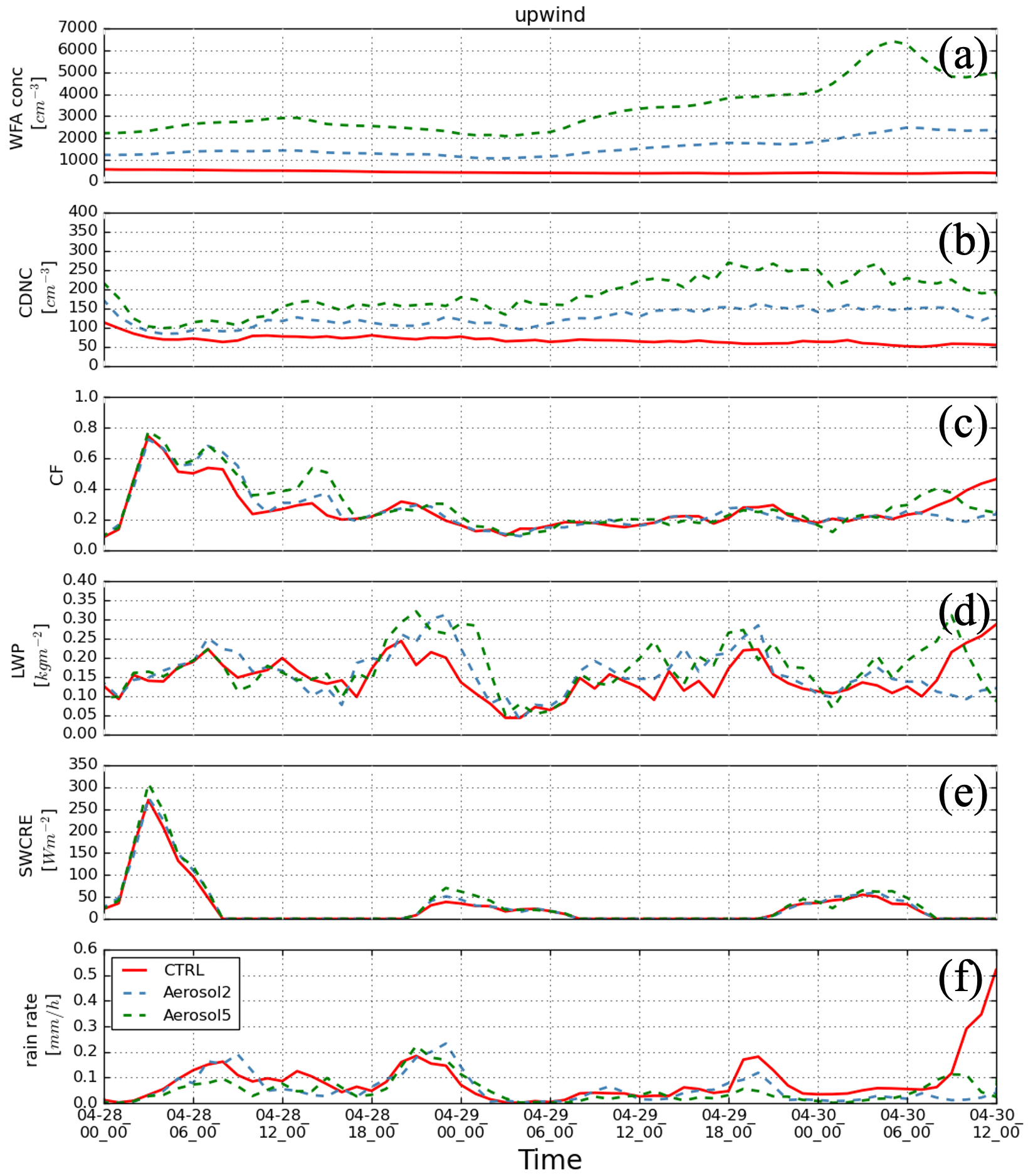
Figure 11 Time series of domain-averaged (a) water-friendly aerosol number concentration, (b) cloud droplet number concentration, (c) cloud fraction, (d) liquid water path, (e) shortwave cloud radiative effect, and (f) rain rate from 1 km resolution with CTRL (solid red lines), Aerosol2 (dashed blue lines), and Aerosol5 (dashed green lines). The target area is over the upwind sub-domain.

5.2 Local aerosol loading

We have also explored the hypothesis that regional aerosol loading may affect the cloud and precipitation properties over the GBR. As shown in Fig. 11a, doubling the surface WFA emission over the GBR (Aerosol2 experiment) results in an increase of ∼700 cm⁻³ (∼122 % increase) in the near-surface WFA number concentration over the upwind sub-domain (from 572 to 1250 cm⁻³), throughout the evolution of the simulation. The increase in WFA emission at the surface also leads to an increase in the atmospheric WFA population to levels above 2 km (Fig. 13a). Pertaining to the Aerosol5 experiment, the near-surface WFA number concentration increases by approximately 1400 cm⁻³ (∼251 % increase), from 572 to 2241 cm⁻³, in comparison to the CTRL (Fig. 11a), as well as an enhancement in the upper-level profile of the WFA concentration (Fig. 13e). A slight time variation in WFA number concentration (WFANC) is seen for both Aerosol2 and Aerosol5, which primarily results from the advection and diffusion of the aerosol during the model integration (Thompson and Eidhammer, 2014). The gradual increase in the WFA number concentration during the last day of the simulation is primarily attributed to the strong inflow with an additional significant amount of aerosols from the southern portion of the GBR when the surface wind changes from easterly to southeasterly (Fig. 4). It is worth noting that a fairly similar increase in the WFANC is also seen over the downwind sub-domain in both aerosol sensitivity experiments (Figs. 12a and 13a, e). Given the predominance of trade wind patterns in this region, this downwind impact is not unexpected.

Figure 12 The same as Fig. 11 but for the downwind sub-domain.

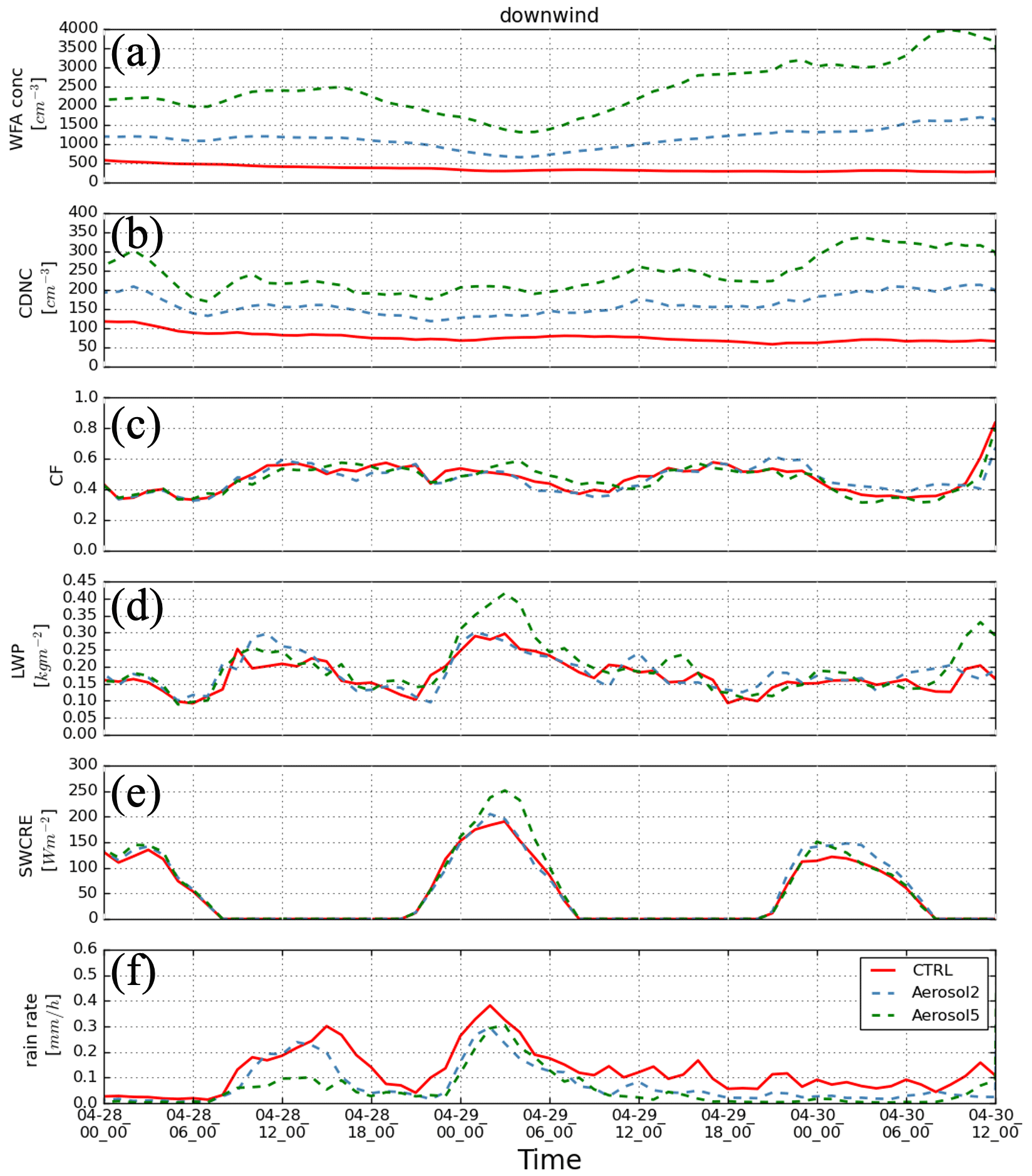
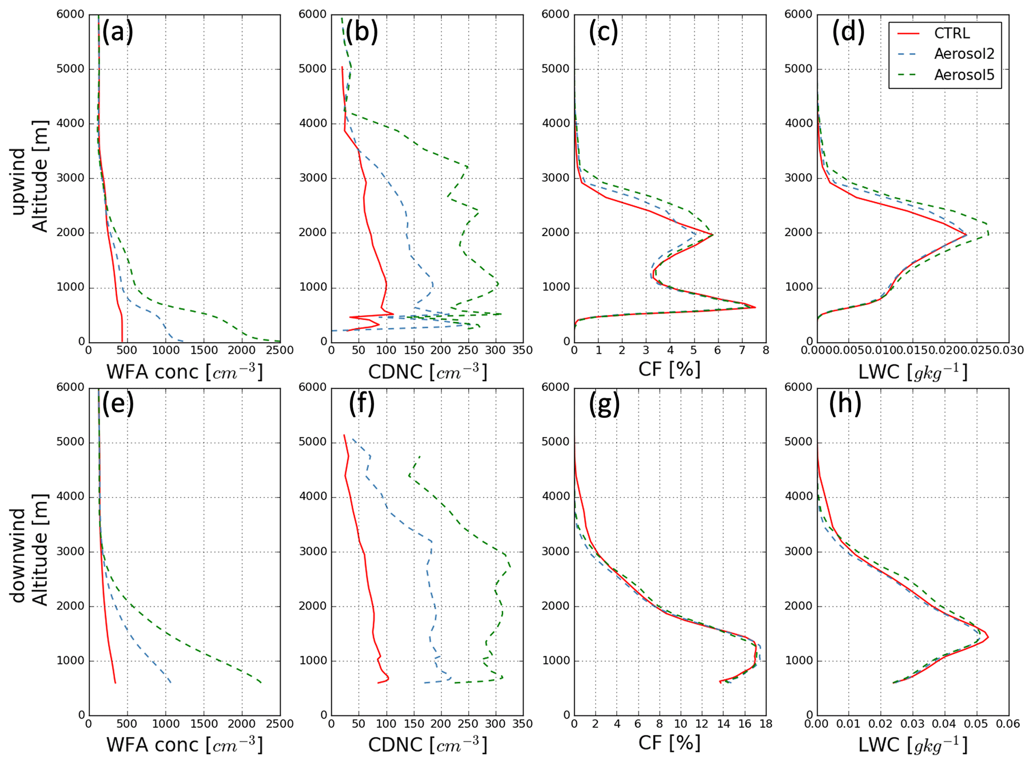
Figure 13 Vertical profiles of (a) domain-averaged water-friendly aerosol number concentration, (b) in-cloud averaged cloud droplet number concentration, (c) domain-averaged cloud fraction, and (d) domain-averaged liquid water content over the upwind sub-domain from CTRL (in red), Aerosol2 (in blue), and Aerosol5 (in green). The analysis is for 60 h simulation time after the spin-up from 00:00 UTC on 28 April to 12:00 UTC on 30 April 2016. Panels (e–h) are the same as (a–d) but for the downwind sub-domain.

Cloud droplet number concentration (CDNC), considered both upwind and downwind, is sensitive to the changes in the atmospheric aerosol number concentration (Figs. 11b and 12b). A higher CDNC corresponding to an increase in the WFA population is evident from the cloud base to the cloud top (Fig. 13b and f), which is consistent with the findings presented in Fiddes et al. (2022). Total CF, however, is found to be essentially unaffected by the changes in the aerosol concentration over both sub-domains (Figs. 11c and 12c). The vertical profile of CF over the upwind sub-domain (Fig. 13c) suggests a slight deepening of the trade cumulus with an increase in domain-averaged CF at cloud top, especially in Aerosol5 experiment (also shown in Fig. 8c). Minimal response is seen at cloud base. This is consistent with an increase in the liquid water path (LWP), which is evident in both the Aerosol2 and Aerosol5 experiments (Figs. 11d and 13d) over the upwind. Looking downwind, even though the CF remains largely unchanged across the altitudes (Figs. 13g and 7b, c), a cloudy layer with higher CDNC could also result in a larger LWP that is likely due to cloud lifetime effects (Albrecht 1989; S. Zhang et al., 2016), as shown in Fig. 12d. Additionally, the cloud radiative effect (CRE) has been considered through the CTRL run and the aerosol sensitivity experiments. CRE is defined as the net radiation flux (downward flux minus upward flux) under all sky conditions minus the net radiation flux under clear-sky conditions and can be applied to both the surface and top of atmosphere (Imre et al., 1996; Bao et al., 2020). Here, in this analysis, it focuses on the shortwave CRE (SWCRE) at the surface, as it represents the effective solar heating of the sea surface. As shown in Figs. 11e and 12e, a rise in SWCRE, though small with a maximum of 50 W m⁻², is evident with an increase in aerosol population over both sub-domains. This is primarily attributed to the higher CDNC, as the cloud reflectance is enhanced with increased droplets number concentration.

As shown in Fig. 9b and c, a reduction in total precipitation is seen in both Aerosol sensitivity experiments, primarily over the downwind mountain area, with a maximum 30 mm difference (∼30 % reduction) noted around the peak precipitation points. This decreased precipitation is evident throughout the simulation hours between the CTRL and aerosol sensitivity runs (Fig. 12f). Relatively small changes (less than 20 mm) in accumulated precipitation are seen over the upwind area, where the decreased accumulated precipitation mainly originates from a few hours in the last day of simulation (Fig. 11f). Although small in magnitude, the warm-cloud precipitation over the GBR is found to show considerable responses to the changes in the local aerosol loading.

Increased CCN concentrations can be expected to produce smaller droplets for a given liquid water content (Twomey, 1977). The smaller cloud droplets can reduce the efficiency of collision and coalescence, which may inhibit precipitation development (Albrecht, 1989). Over the GBR, sensitivity experiments in this study consistently indicate that cloud microphysical properties, including CDNC and LWP, and precipitation respond strongly to changes in the local WFANC. A significant rise in CDNC (∼2.5X in Aerosol5) is correlated with an increase in the aerosol population that is seen over the GBR and predominantly leads to suppressed precipitation (up to a 40 mm reduction in total precipitation) over both upwind and downwind areas. While the total CF shows less sensitivity to the aerosol perturbations, it is worth noting that the aerosol sensitivity experiments also show evidence of deepened trade cumulus over the upwind region, which will increase the LWP and the SWCRE. Note that fluctuations in LWP response are observed throughout the simulation. Previous studies have shown that multiple processes (e.g., cloud formation processes, evaporation, and precipitation) play a role in determining the LWP response to aerosol perturbations (Han et al., 2002). In addition, meteorological conditions (e.g., relative humidity) could strongly modulate the LWP droplet number–concentration relationship (Gryspeerdt et al., 2019). A notable downwind effect featuring by a significant reduction in surface precipitation is simulated when changing the surface aerosol emissions over the GBR.

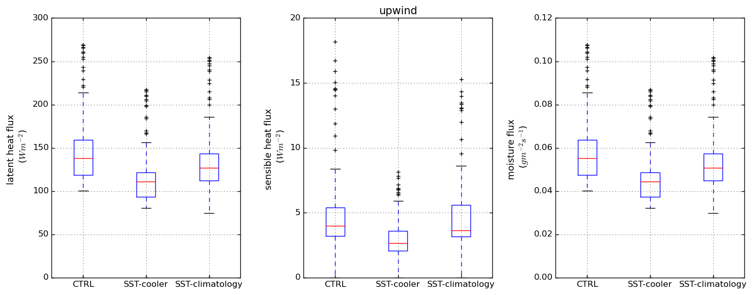
Figure 14 Boxplots showing the comparison of latent heat flux, sensible heat flux, and moisture flux from 1 km resolution simulation with CTRL, SST-cooler, and SST-climatology. The analysis is for the 60 h simulation period and over the upwind sub-domain.

It should be noted that how convection may interact with changes in aerosol is still a large source of uncertainty (Tao et al., 2012), and experiments in this study only focus on perturbing the water-friendly aerosol loading over the GBR. Previous studies have shown that the thermodynamic environment is strongly modulated by the large-scale forcing, whose impact on the cloud field might surpass that of local aerosol perturbations (Dagan et al., 2018; Spill et al., 2021). Spill et al. (2021) show that the response of cumulus cloud and precipitation to the aerosol perturbation is much stronger in the idealized simulations without the large-scale forcing. This suggests a potentially limited effect of aerosols on cumulus cloud fields in the realistic condition due to the predominant influence of large-scale forcing. The nature variability of the marine shallow clouds and precipitation process could also explain some of the differences between the CTRL and aerosol sensitivity runs.

5.3 Local SST forcing

In this section, we have explored the sensitivity of cloud and precipitation properties over the GBR in response to the local SST changes. A reduction in CF is noted over the upwind in the SST-cooler run, with the most notable difference apparent at lower altitudes (Fig. 8e). Over the downwind sub-domain, the CF has only a small difference between the CTRL and SST-cooler experiments (Fig. 7e). However, a decrease in the accumulated precipitation is discernible over downwind points with the peak accumulated precipitation (Fig. 9e). Similar but more variable findings are evident from the SST-climatology experiment. Figure 7f shows small but more complex changes in CF in the downwind area with associated positive and negative changes in accumulated precipitation (Fig. 9f). These variable impacts are likely due to the non-uniform (positive and negative) changes in SST associated with the differences between the CTRL and SST-climatology runs. (Fig. S1). The downwind effect on precipitation is similarly discernible in the SST-climatology; however, there are no noteworthy results related to the cloud fraction (Fig. 7f).

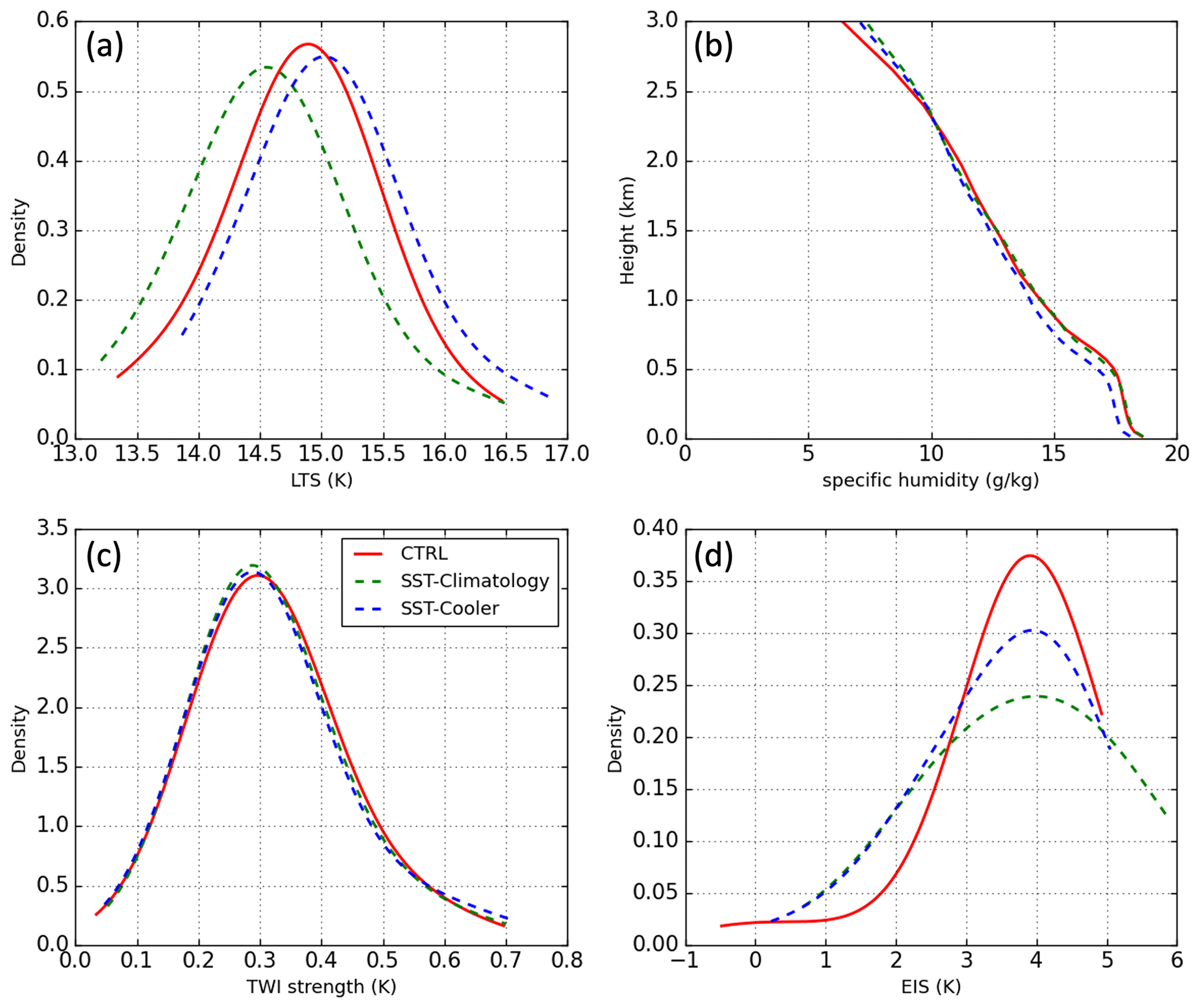
Figure 15 PDF distribution of the (a) LTS, (b) vertical profile of humidity, (c) TWI strength, and (d) EIS over the upwind area. The analysis covers the whole 60 h simulation period after the spin-up time. Solid red lines represent results from CTRL, and dashed lines are for the SST sensitivity experiments.

Theoretically, a warmer SST will likely provide more water vapor in the atmosphere through increased surface latent heat fluxes (Rieck et al., 2012; Vogel et al., 2016). The increased atmospheric water vapor, under such conditions, will consequently induce more rainfall at local and downstream regions. A decrease in surface heat flux and moisture flux is noted in the SST-cooler experiment (Fig. 14), preventing the formation and development of the shallow cloud. There is a relative minor difference in averaged surface flux between the CTRL and the SST-climatology experiment (Fig. 14) that is potentially associated with non-uniform modifications in SST (Fig. S1). However, a notable wide distribution of surface flux is likely contributing to the complex response of cloud and precipitation in the SST-climatology experiment (Figs. 7f and 9f). It is also suggested that with a warmer SST, the boundary layer becomes more humid, which becomes destabilized by increased clear-sky radiative cooling, driving more cumulus convection (Narenpitak and Bretherton, 2019; Wyant et al., 2009; Narenpitak et al., 2017). In this study, the SST-cooler experiment reveals a more stable lower troposphere (Fig. 15a) compared to CTRL, which inhibits the formation of trade wind clouds. A slight unstable condition is seen in the SST-climatology experiment, which likely contributed to the warmer pool at the upwind ocean, driving more variable changes in cloud and precipitation (Figs. 7f and 9f). Another factor that controls the cloud amount is the free tropospheric humidity (Bretherton et al., 2013; Eastman and Wood, 2018). It is suggested that drier air at the level of the free troposphere causes more entrainment drying, depleting the boundary layer cloud water. As shown in Fig. 15b, slightly drier conditions are seen at the lower level below 1 km in the SST-cooler experiment; however, there is no significant difference near the free troposphere (2.5 km). Large-scale circulation and local processes play important roles in driving the thermodynamic profiles (Nygård et al., 2021). Considering the magnitude of adjustment in surface temperature, the changes may not be felt by the upper atmospheric levels. This limited impact could be further diminished by large-scale atmospheric dynamics. Nevertheless, drier conditions at the lower level are likely contributing to the stabilized boundary layer simulated in the SST-cooler experiment. Finally, two measures of the inversion strength, specifically TWI strength and EIS, have been examined with the SST experiment. The results show that inversion strength is not a predominant factor impacting the interactions of trade clouds and local SST forcing. As discussed above, the inversion strength is more likely to be influenced by synoptic to larger-scale atmospheric processes (Milionis and Davies, 2008), which have the potential to eclipse the impact of local forcings.

Over the tropics, the SST has been noted in several studies to be a key factor controlling the location of rainfall over various timescales (Lu and Lu, 2014; Jo et al., 2019; Wu et al., 2009; Wu and Kirtman, 2007). Takahashi and Dado (2018) highlight the impact of local and/or nearby SST on local and regional climate. In particular, they found that warmer local SST results in greater rainfall over the downstream land region in the mid-latitudes based on observational dataset, which suggests strong air–sea coupling processes. Numerical sensitivity experiments in this study to some extent show consistent results, indicating that precipitation over the GBR shows a response to the underlying SST conditions, though the effect is weak on the scales considered here. A downwind effect on the precipitation has been found over the Wet Tropics. Sensitivity of cloud fraction in response to SST variation is seen over the water area, though the magnitude is minor in comparison with the major orographic impacts. The relationship between cloud fraction and SST at the lower levels have been found to largely depend on the type of cloud and its height (Cesana et al., 2019). A stronger response of “lower-top” shallow-cloud properties (i.e., stratocumulus) to the changes in SST is noted in Cesana et al. (2019) in comparison with “higher-top” shallow clouds (e.g., cumulus). As such, many minor responses to the changes in SST are expected when considering cloud fields with higher cloud tops. In this study, instances of simulated cloud fields with cloud tops over 3 km could largely contribute to the variety in the responses to SST forcing.

Overall, simulations in this study suggest that warm-cloud precipitation over the GBR is sensitive to the underlying local SST forcing, though the responses are weak on the scales considered in this study. The lower troposphere stability and surface heat and moisture flux likely primarily explain most of the responses of trade cumulus over the GBR to local SST forcing. This work supports the important role of local SST in the regional climate over the GBR, but further work toward understanding the synoptic and thermodynamic background and air–sea coupling processes is necessary to help elucidate the mechanisms involved.

6 Summary and conclusions

A primary aim of this research is to study the sensitivity of trade cumulus precipitation to different local forcings over the GBR using a case study of an orographic precipitation event associated with low-level trade cumulus at the end of April 2016. The selected days for the simulations are characterized by well-defined cumulus and stratocumulus under the trade wind regime without any overlying high clouds. These trade cumuli are observed to generate precipitation over the Wet Tropics around Townsville.

The large-scale meteorology is well captured in the CTRL simulation in terms of the location, duration, and magnitude of the surface pressure system and wind fields. Comparison of the upper-air profiles from both Townsville and Willis Island sounding stations showed good agreement in wind speed, wind direction, and temperature profiles. The CTRL simulation also demonstrated a considerable level of skill in simulating both the spatial distribution and the intensity of precipitation over the Wet Tropics as compared to ground observations.

Sensitivity experiments are conducted to investigate the sensitivity of trade cumulus and precipitation in response to the local forcings. Major findings from the sensitivity analysis presented in this study are summarized as follows.

• Reducing the elevation above 300 m by 75 % decreases the cloud fraction and accumulated precipitation over the Wet Tropics, including both downwind and upwind areas. Weaker vertical velocity, low-level wind convergence, and more stable lower troposphere are generated in the Topo300 run over the downwind sub-domain, suggesting their crucial role in rainfall production. The reduced TWI base height in the Topo300 run is found to limit the cloud precipitation development over the upwind water area.

• Cloud microphysical properties, including CDNC, LWP, and precipitation, are sensitive to the changes in atmospheric aerosol population over the GBR. Higher CDNC and LWP correlated to increased aerosol number concentration leads to a rise in SWCRE, though the magnitude is small over both sub-domains. Although CF remains largely unchanged, a deepened cloud is evident over the upwind when WFANC is increased. A downwind effect on cloud and precipitation properties is further noted.

• Cloud fraction and total precipitation over the GBR show a small response to the underlying local SST forcing. A reduction in cloud fraction is noted over the upwind water area when the initial SST is reduced, but any difference is negligible over the downstream orographic region. There is a decrease in the accumulated precipitation in the SST sensitivity experiments over downwind grids where the peak accumulated precipitation generated. These small decreases in cloud fraction and accumulated precipitation are likely associated with the consistently decreased surface flux and stabilized lower troposphere in the SST experiments.

It should be noted that a limitation of this present study is the choice of model set-up in relation to the aerosol representation. In this work, the microphysics scheme simply treats aerosol categories into “water-friendly” and “ice-friendly” aerosols. While using a more comprehensive representation of aerosol sources in the model is desirable for a more complete understanding of the complex interactions between aerosols and atmospheric processes (Ghan et al., 2012; Wang et al., 2013), these aerosol-resolving models commonly come at a significant computational cost and are simply unaffordable at a cloud-resolving resolution over a large domain. The primary aim of this study is to better understand the first-order impacts of local forcings on the clouds and precipitation over the GBR, which is the first step towards a more comprehensive investigation of aerosol–cloud–climate interactions. This research requires a large domain at reasonably high resolution to properly capture the complex interactions between the large-scale meteorology and local forcings, which are critical for trade wind cloud formation (e.g., Vogel et al., 2020; Bretherton and Blossey, 2017). Although far from perfect, the use of the (simplified) aerosol-aware Thompson and Eidhammer (2014) scheme in a convection-permitting configuration is a reasonable middle ground to address these two critical needs. Note that a combination of sulfates, sea salts, and organic matter is found to represent a significant fraction of known CCN and are found in abundance in clouds worldwide (Thompson and Eidhammer, 2014). Therefore, while it would be an interesting (and important) topic for a different project, a precise understanding of aerosol sources, amounts, and composition is beyond the scope of the present study.

It might be considered desirable to employ the higher-resolution modeling such as large-eddy simulation (LES) to better resolve the details of the complex cloud and precipitation processes. Although simulations in this study are at a lower resolution than needed to resolve detailed cloud processes such as entrainment and convective aggregation, they are at a high enough resolution to explicitly represent convection while allowing for a considerably larger domain size at an affordable computational cost. The significance of a large domain size has been demonstrated in accurately representing the mesoscale organization of trade wind cumulus (Vogel et al., 2020; Bretherton and Blossey, 2017). High-resolution LES is not currently possible at the larger domain sizes considered in this study, and therefore it is difficult to use it to study detailed interactions between orography, cloud organization and variation, and large-scale forgings. In addition, it is acknowledged that presenting statistical significance values is inherently challenging in case studies due to the unique nature of each case and limited samples. However, it is believed that the careful consideration of the model's set-up, combined with a thorough comparative analysis, allows this study to present the findings with a reasoned level of confidence.

Although a range of responses of cloud and precipitation to the local forcings are produced across the GBR in simulations presented in this study, it is recognized that ensemble analysis is necessary in the future to better represent the natural variability of these trade clouds and precipitation properties. Subsequent research endeavors should also consider the influence of additional local forcings, such as wind shear (Yamaguchi et al., 2019), in the modulation of cloud and precipitation dynamics within trade wind regimes. Li et al. (2014) also suggests that downdrafts at the cold pool boundary play an important role in the development of trade wind cumuli. These studies highlight the complex nature of atmospheric dynamics in trade wind cumuli and emphasize the necessity of comprehensive investigations into these additional variables to enhance our understanding of cloud and precipitation in trade wind cumuli in the GBR region. In situ observations will also be necessary to help investigate the detailed lifecycle of these low-level clouds and the development of the topographic precipitation. Furthermore, there is a need to carry out case studies during the time of intense SST increases that may induce thermal coral bleaching over the GBR. Nevertheless, this analysis sheds some light on understanding the interactions between trade wind cumuli and local forcings across the GBR and Wet Tropics, where the importance of the local low-level cloud in thermal coral bleaching has recently been identified. This study also holds significant relevance for assessing the comprehensive effects of proposed climate intervention techniques, such as marine cloud brightening, on the thermal balance of the GBR region. While this study provides specific insights into the sensitivity of trade cumulus precipitation over the GBR in a particular time frame, its methodologies and findings have broader applications. It offers valuable insights that can be extrapolated to other regions characterized by pristine trade wind and trade cumulus conditions, contributing to a more comprehensive understanding of regional climate dynamics.