the Creative Commons Attribution 4.0 License.
the Creative Commons Attribution 4.0 License.
 | 07 May 2024
Potential of using CO2 observations over India in a regional carbon budget estimation by improving the modelling system
Vishnu Thilakan
Jithin Sukumaran
Christoph Gerbig
Haseeb Hakkim
Vinayak Sinha
Yukio Terao
Manish Naja
Monish Vijay Deshpande
Devising effective national-level climate action plans requires a more detailed understanding of the regional distribution of sources and sinks of greenhouse gases. Due to insufficient observations and modelling capabilities, India's current carbon source–sink estimates are uncertain. This study uses a high-resolution Lagrangian transport model to examine the potential of available CO2 observations over India for inverse estimation of regional carbon fluxes. We use four different sites in India that vary in the measurement technique, frequency and spatial representation. These observations exhibit substantial seasonal (7.5 to 9.2 ppm) and intra-seasonal (2 to 12 ppm) variability. Our modelling framework, a high-resolution Weather Research and Forecasting Model combined with the Stochastic Time-Inverted Lagrangian Transport model (WRF–STILT), performs better in simulating seasonal (R2=0.50 to 0.96) and diurnal (R2=0.96) variability (for the Mohali station) of observed CO2 than the current-generation global models (CarboScope, CarbonTracker and ECMWF EGG4). The seasonal CO2 concentration variability in Mohali, associated with crop residue burning, is largely underestimated by the models. WRF–STILT captures the seasonal biospheric variability over Nainital better than the global models but underestimates the strength of the CO2 uptake by crops. The choice of emission inventory in the modelling framework alone leads to significant biases in simulations (5 to 10 ppm), endorsing the need for accounting for emission fluxes, especially for non-background sites. Our study highlights the possibility of using the CO2 observations from these Indian stations for deducing carbon flux information at regional (Nainital) and suburban to urban (Mohali, Shadnagar and Nagpur) scales with the help of a high-resolution model. On accounting for observed variability in CO2, the global carbon data assimilation system can benefit from the measurements from the Indian subcontinent.
- Article
(4446 KB) - Full-text XML
-
Supplement
(10898 KB) - BibTeX
- EndNote


The global terrestrial ecosystem acts as a significant carbon sink. A decrease in sink capacities accelerates global warming as a consequence of the increased atmospheric emission fraction (airborne fraction). How the terrestrial carbon sink capacity responds to the rate of atmospheric greenhouse gas increase remains uncertain, implying large uncertainties in future climate predictions. Further, significant uncertainties exist in our estimations of the magnitude and spatial distribution of carbon fluxes between land, atmosphere and the oceans (Friedlingstein et al., 2022). These estimates are particularly critical to devising effective mitigation plans for climate change. The carbon budget estimation system must sufficiently represent the complex exchange processes operating at different spatial and temporal scales to address the above key shortcoming.
India needs an accurate estimation of its carbon sources and sinks to achieve its nationally determined contribution (NDC) goals (https://unfccc.int, last access: 25 March 2023) through emission reduction. The bottom-up approach is widely used to estimate carbon fluxes based on our prior knowledge of the processes determining the fluxes, such as vegetation, land types and fossil fuel usage statistics. However, these estimates are often characterised by large errors due to various factors, including the reliability of statistical reports, the accuracy of flux estimation approaches and the desired spatiotemporal resolution. An inverse-modelling framework (top-down approach, Enting, 2002) encompassing atmospheric transport models and observations of atmospheric carbon concentrations has the potential to improve bottom-up-approach-based estimates of the source–sink distribution of carbon globally (e.g. Rödenbeck et al., 2003; Peters et al., 2007; Inness et al., 2019) and at regional scales (e.g. Gerbig et al., 2009; Broquet et al., 2013; Pillai et al., 2016). There have been a few recent inverse-modelling-based attempts to estimate the carbon fluxes over the South Asian region using in situ and satellite observations (e.g. Patra et al., 2013; Thompson et al., 2016; Ganesan et al., 2017; Philip et al., 2022; Sijikumar et al., 2023); however, these studies are limited by the general paucity of observational data with sufficient temporal and spatial coverage over the region.
In situ observations are essential for the tropics because satellite observations representing the entire atmospheric column cannot always detect signatures from small-scale surface flux variations. Moreover, one may expect significant data gaps in satellite measurements, depending on the season, due to clouds and moist convection. Recently, more greenhouse gas (GHG) monitoring stations have been set up over India by different research initiatives (e.g. Tiwari et al., 2014; Lin et al., 2015; Mahesh et al., 2015; Chandra et al., 2016; Jain et al., 2021; Nomura et al., 2021; Sijikumar et al., 2023). High-frequency observations with diurnal and synoptic variations provide information on the regional sources and sinks for atmospheric CO2, which are influenced by mesoscale atmospheric transport (Law et al., 2002; Gerbig et al., 2003; Geels et al., 2004; Lin et al., 2004; Lauvaux et al., 2008). CO2 anomalies generated remotely can also affect these observation sites through horizontal advection. Law et al. (2002) have suggested that the use of high-frequency observation can aid in reducing the uncertainty in inverse estimates, similar to using a larger observation network with low-frequency observations. However, measurements obtained from an observation site close to a variable source or meteorologically complex areas are difficult to represent in the transport models used for inversions. These factors must be considered while developing observation sites that can be used for inverse optimisation. Due to the unavailability of consistent long-term observations representing the regional fluxes, none of the current-generation global carbon assimilation systems utilise CO2 observations from the Indian region. Additionally, to utilise the potential of these observations through inverse modelling, we need to improve our understanding of the processes driving high-frequency variability in these measurements (Geels et al., 2004). That is, sufficient improvement in modelling capabilities is required over the Indian region.
The skill of the model is determined by how well it can simulate the variability in atmospheric CO2 concentration. The model–observation mismatch in atmospheric CO2 concentrations emerges due to the combined effect of uncertainties in the transport processes and the improper representation of CO2 flux variability. The accurate representation of the planetary boundary layer (PBL) height is also crucial for the simulation of the tracer distribution in the boundary layer and its dynamics (e.g. Gerbig et al., 2008). Most current-generation carbon flux estimations over India are derived from global carbon estimates, which utilise coarse-resolution transport models (e.g. Rödenbeck et al., 2003; Peters et al., 2007; Inness et al., 2019) for their simulations. However, atmospheric CO2 exhibits strong spatiotemporal variations such that the transport models need a horizontal resolution higher than 30 km to represent the variability (Gerbig et al., 2003). Similarly, local and large-scale convections play a major role in distributing atmospheric tracer concentrations (Gerbig et al., 2003) vertically, which is difficult to simulate in tropical regions (Thompson et al., 2014). Fine-scale features are better resolved when the horizontal resolution of transport models is increased (Geels et al., 2007; Tolk et al., 2008; Agustí-Panareda et al., 2019). Thilakan et al. (2022) showed that considerable representation errors exist when we use coarse-resolution transport models for inverse optimisation over India, and the representation error tends to decrease when we increase the horizontal resolution. The seasonally reversing monsoon circulation pattern and complex topography complicate regional atmospheric transport, influencing the vegetation patterns and agricultural practices over the region. Hence, an adequate representation of the atmospheric CO2 distribution over India relies on a modelling system that can operate at a high spatial and temporal resolution and has the ability to simulate all the essential underlying processes. There are increasing efforts in recent years to constrain the regional CO2 fluxes over India via inverse-modelling frameworks (Halder et al., 2022; Philip et al., 2022; Sijikumar et al., 2023). However, when assimilating regional measurements in the inverse-optimisation framework, it is crucial to investigate how effectively the forward-modelling system reproduces the observed variations associated with fine-scale transport and local influences at various timescales. This is because considerable model–data mismatches due to transport errors can lead to large uncertainties in the estimated fluxes.
This study focuses on assessing the potential of four available observations over India to be employed in future high-resolution inverse-modelling frameworks to optimise regional CO2 fluxes. We analyse the variability and representativeness of CO2 observations from each station. Observations with high variability, often due to the influence of local flux variations, may not be suitable for regional flux optimisations but can provide important information about local emission sources. Further, we examine the capability of a high-resolution modelling framework based on the Lagrangian particle dispersion model (LPDM) to simulate CO2 variability over these observation sites. We follow the receptor-oriented framework described in Gerbig et al. (2003) using an LPDM called the Stochastic Time-Inverted Lagrangian Transport (STILT) model (Lin et al., 2003). The CO2 observations used in this study were taken from the near surface using different measurement techniques at different frequencies. We assess the usability of these measurements in the inverse framework when utilising the high-resolution (e.g. WRF–STILT; Weather Research and Forecasting Model) modelling system to optimise carbon fluxes. We quantify the model uncertainties and compare them with some of the existing coarse-resolution models.
This paper is organised as follows: Sect. 2 briefly describes the modelling framework employed in this study. In Sect. 3, we provide the details of CO2 measurements and global reanalysis data used in this study. Section 4 deals with the methods used for assessing the model skill in capturing observed variability. Section 5 presents the observed CO2 variability across India, investigating how well STILT and global models could capture these variations. In Sect. 6, we further discuss the potential of using these observations in the future inverse-modelling system, taking into account the current limitations of our modelling system. The conclusions are presented in Sect. 7.
A receptor-oriented analysis framework was designed to quantify the sensitivity of the atmospheric CO2 concentrations (influence functions) at measurement locations (receptors) to the surface fluxes in the upwind regions or boundary conditions and thereby interpret the atmospheric signatures of the surface processes. These influence functions (footprints) can be considered equivalent to the adjoint of the Eulerian transport model. This STILT modelling framework utilises meteorology from an Eulerian transport model, surface fluxes from biospheric models or inventories, and boundary conditions from global reanalysis products to simulate the atmospheric CO2 concentration at receptor locations. The boundary conditions are intended to provide the background and influence of remote fluxes on the observations. In this study, the Weather Research and Forecasting (WRF) Model is used to simulate meteorology at a horizontal resolution of 10 km × 10 km and a temporal resolution of 1 h. Using STILT has the advantage of simulating CO2 variability down to spatial scales that are slightly smaller than the grid size of the meteorological fields used (Lin et al., 2003; Gerbig et al., 2003). Because it employs a backward-time simulation strategy, it is more computationally cost-effective than an alternative forward-time simulation (Lin et al., 2003), at least for data-sparse situations with only a few observational sites.
We simulated CO2 concentrations at the measurement locations using the WRF–STILT modelling framework. A detailed description of the WRF–STILT system can be obtained from Nehrkorn et al. (2010). The STILT is a widely used LPDM to determine the influence of surface emissions at a receptor location by simulating the transport in the near field (i.e. the surface that PBL air has come into contact with before arriving at the measurement location) (e.g. Lin et al., 2003; Gerbig et al., 2003; Nehrkorn et al., 2010; Pillai et al., 2011; Maier et al., 2022). The STILT model utilises the mean advection scheme used by the Hybrid Single-Particle Lagrangian Integrated Trajectory (HYSPLIT) model (Stein et al., 2015). The turbulent motions are modelled as a Markov chain process (Lin et al., 2003). The mean wind is represented by interpolating the wind fields from numerical weather prediction models or reanalysis data (from the WRF model in this study) into the sub-grid location of the particle. STILT simulates the transport by following the backwards-in-time evolution of an ensemble of particles (representing air parcels of equal mass) from receptor locations using mean winds and turbulent motions. The most critical meteorological variables required for trajectory calculations are vertical profiles of horizontal and vertical wind components (Nehrkorn et al., 2010).
In the STILT model, changes in the atmospheric CO2 concentration, ΔC(xr,tr) at the observation site at xr and time tr, can be derived as follows:
where S(x,t) is a volume source–sink (in units of ppm h−1) and is the influence function for the receptor location which quantitatively links sources and sinks to concentrations (in units of m−3). The quantification of the time volume integration of the influence function is achieved by counting the total length of time that each released particle p spends in a volume element during a time step m and normalising to the number of particles released Ntot (Lin et al., 2003).
The link between surface fluxes (in units of mol m−2 s−1) and a volume source–sink S(x,t) is established by diluting the surface tracer flux into an atmospheric column of height h, in the assumption that the turbulent mixing below this height is strong enough to thoroughly mix the surface flux from ground to h within one model time step m. Here, h is set to half of the PBL height, and the PBL height is calculated internally by STILT using meteorological inputs provided by WRF. These WRF meteorological simulations (temperature, moisture and wind) are compared reasonably well (R2>0.75) with observations (Mathew et al., 2024). STILT computes the PBL height with the help of a modified Richardson number as described in Vogelezang and Holtslag (1996). The relation between and S(x,t) is summarised in Eq. (3) as follows:
where mair is the molar mass of air and is the average air density. From the above equations (Eqs. 1, 2 and 3), the contribution of emission fluxes from each surface grid cell (i,j) and time step m to the total CO2 enhancement ΔC(xr,tr) at receptor location can be obtained as
Here, is known as the “footprint” which links the CO2 surface fluxes to CO2 concentration changes at the observation site as mentioned before. The total CO2 concentration enhancement ΔC(xr,tr) at the observation site is obtained by summing over all the grid cells (i,j) and time (m).
We released 100 particles from every receptor location to calculate the back trajectories with a maximum backward time of 120 h. This period is set by estimating the approximate time required for all particles to exit the model domain. We used the time-averaged, mass-coupled velocity fields from the WRF model to avoid mass violation in STILT. The initial and boundary conditions for WRF are obtained from the ERA5 reanalysis dataset of the European Centre for Medium-Range Weather Forecasts (ECMWF) (Hersbach et al., 2018a, b). The WRF simulations over the domain are generated for 2017. The detailed description of the WRF model set up over the Indian domain used for this study can be obtained from Thilakan et al. (2022). The evaluation of the WRF model simulations over India shows a good agreement with observations (e.g. Hariprasad et al., 2014; Boadh et al., 2016; Sivan et al., 2021; Mathew et al., 2024). The footprints were calculated based on Eq. (4), which were dynamically gridded to a maximum resolution of 10 km × 10 km.
The biosphere flux distribution over the domain was generated using a biospheric model called the Vegetation Photosynthesis and Respiration Model (VPRM) (Mahadevan et al., 2008). VPRM calculates gross ecosystem exchange (GEE) and ecosystem respiration (Reco) using WRF meteorological fields and MODIS (Moderate Resolution Imaging Spectroradiometer) data from Terra and Aqua satellites. Biospheric fluxes are generated at a horizontal resolution of 10 km × 10 km over the domain. These fluxes were utilised to calculate the atmospheric CO2 contribution by the biosphere over the receptor locations (termed as CO). Anthropogenic CO2 fluxes were prescribed from three different inventories to represent anthropogenic contribution and also to examine the impact of emission differences in CO2 simulations over the Indian domain. Anthropogenic emission fluxes from the Emissions Database for Global Atmospheric Research (EDGAR), Open-source Data Inventory for Anthropogenic CO2 (ODIAC) and Integrated Carbon Observation System global anthropogenic CO2 emissions (hereafter referred to as ICOS) were used in this study. The EDGAR inventory (v7.0; Crippa et al., 2018, 2022) provides anthropogenic fluxes at a horizontal resolution of 0.1° × 0.1° for every year. ODIAC (v2020; Oda and Maksyutov, 2020; Oda et al., 2018) has a higher spatial resolution of 1 km × 1 km but is available only at a monthly timescale. ICOS (v2019; Karstens et al., 2019; Janssens-Maenhout et al., 2019) is based on EDGAR v4.3 and BP statistics with a horizontal resolution of 0.5° × 0.5° and an hourly temporal resolution. All these datasets were interpolated into model resolution, conserving mass. The model included the effect of global CO2 variability over the domain from boundary conditions (also known as background signal, CO) and was added to the local CO2 mole fraction (resulting from local fluxes) within the model domain to compare with the observations. In this study, we have used two different global reanalysis products separately as boundary conditions to understand the influence of boundary conditions on the total CO2 mole fraction. We used Jena CarboScope (version s10c_v2020; Rödenbeck et al., 2003) and the ECMWF Copernicus Atmosphere Monitoring Service (CAMS; version EGG4; Agustí-Panareda et al., 2023) as boundary conditions for this study (see Sect. 3.2). We do not include the contribution from oceanic fluxes, as its influence on these stations is very negligible (∼0.001 ppm, figure not shown). We incorporate the influence of biomass burning separately over Mohali during the biomass-burning emission season (see Sect. 6.1 for a detailed discussion).
That is, the total atmospheric CO2 concentration (atmospheric CO2,tot) was calculated by adding the background (CO2,bck), biospheric (CO2,bio) and anthropogenic (CO2,ant) terms together to compare with the observations. The atmospheric CO2 concentration at the measurement location is given by
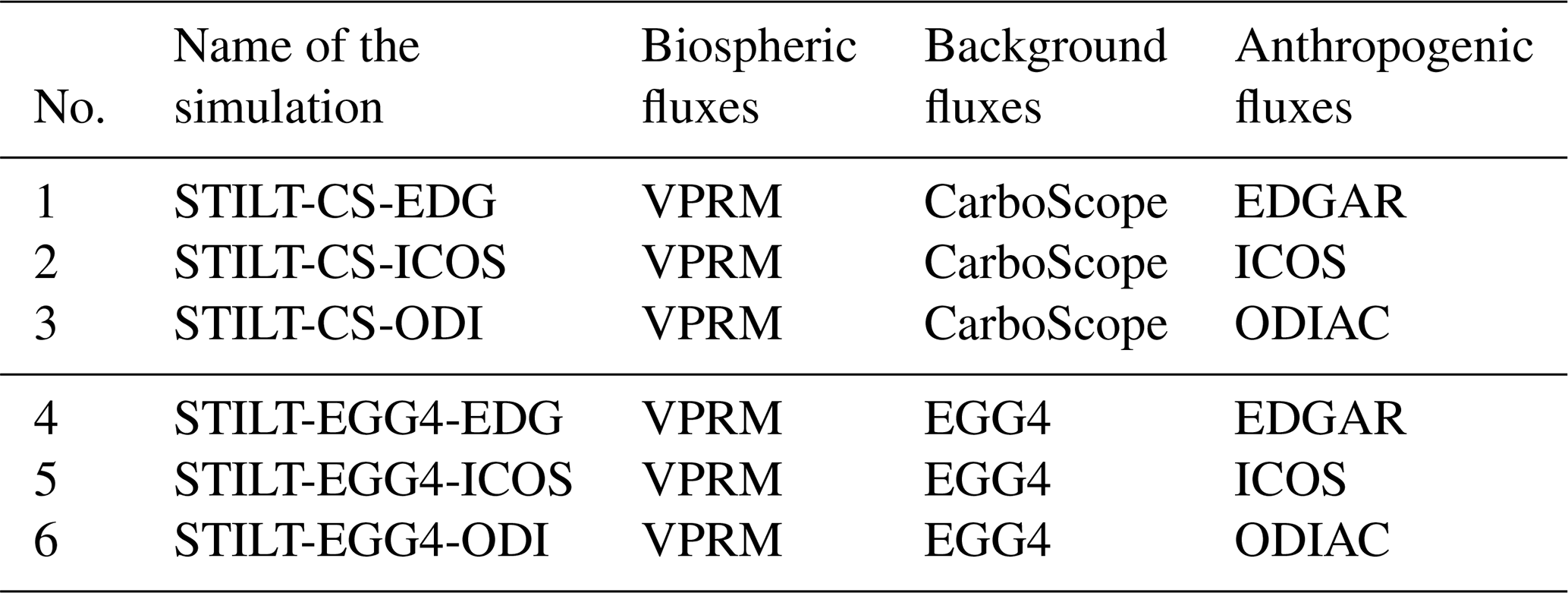
Atmospheric CO2 mixing ratios at the measurement locations were retrieved at a temporal resolution of 3 h. Since we used two different boundary conditions and three different anthropogenic fluxes for the WRF–STILT simulations, we have a set of six simulations (see Table 1) over each observation site. WRF–STILT simulations are hereafter simply referred to as STILT simulations in this article. The simulations with CarboScope (CS) as background are represented as STILT-CS-EDG (EDGAR as anthropogenic flux), STILT-CS-ICOS (ICOS as anthropogenic flux) and STILT-CS-ODI (ODIAC as anthropogenic flux) in this paper. Similarly, simulations with CAMS EGG4 (EGG4) as background are represented as STILT-EGG4-EDG (EDGAR as anthropogenic flux), STILT-EGG4-ICOS (ICOS as anthropogenic flux) and STILT-EGG4-ODI (ODIAC as anthropogenic flux).
Table 1A brief description of different WRF–STILT simulations and their input fluxes used in the study.
3.1 CO2 observations over India
We used atmospheric CO2 observations for 2017 from four measurement sites located in Mohali, Nainital, Shadnagar and Nagpur (see Fig. 1) to assess their temporal variability. The sites were chosen based on the availability of their long-term measurements to the research team. Also, we examined how well the STILT simulations capture these variations.
We used continuous hourly measurements of CO2 using the Picarro CRDS (cavity ring-down spectroscopy) instrument at the Mohali station. Atmospheric CO2 mole fractions are measured at 20 m height above ground level (a.g.l.). The measured CO2 mixing ratios have an overall uncertainty calculated based on the root mean square propagation of individual uncertainties, such as the accuracy error of gas standard (2 %), 2σ instrumental precision error (0.1 % for CO2) and flow reproducibility (2 %), resulting in a measurement uncertainty of less than 4 %. The limit of detection for CO2 is reported to be better than 0.5 ppm (Chandra et al., 2017). The Mohali station is situated in a suburban area (30.67° N, 76.73° E; 310 m a.s.l.) in the northwestern part of the Indo-Gangetic Plain (IGP), close to the city of Chandigarh (Sinha et al., 2014; Pawar et al., 2015). The instrument facility is housed inside the campus of the Indian Institute of Science Education and Research Mohali (IISER Mohali). More details about the measurement techniques employed for Mohali observations are available from Chandra et al. (2017). Mohali is in the proximity of three cities (Chandigarh, Mohali and Panchkula) with a population of more than 100 000 at a distance of a few kilometres in the northeastern direction, among which Chandigarh has a population of nearly 1 million. STILT footprints show that the predominant wind direction towards the observation site is northwest, except during the monsoon season, in which the wind comes in the southeastern direction (Fig. S1 in the Supplement). The northwestern region of Mohali is dominated by agricultural and other rural land use patterns (Kumar and Sinha, 2021). Agricultural emission activities like residue burning can be expected in this region during the April–May and October–November period (Sinha et al., 2014). Local influences on the measurements from the residents of IISER Mohali are expected to be minimal since the measurement facility is located in the upwind direction of the potentially local sources inside the campus.
Weekly flask measurements of atmospheric CO2 mole fractions from the Nainital observation site are used here (Terao et al., 2022). The Nainital observation site is located at the Aryabhatta Research Institute of Observational Sciences (ARIES) (29.36° N, 79.46° E; 1940 m a.s.l.; Nomura et al., 2021). Since the measurement location is near the Himalayan mountain range, Nainital is considered a background site representing northern Indian GHG distribution with some influence from anthropogenic activities, including biomass burning during spring and autumn months when air mass stays for a longer duration over northern India (Sarangi et al., 2014; Nomura et al., 2021). The inlets for the air samples are mounted at a height of 7 m a.g.l. Weekly flask samples were collected at 14:00 LT (local time) and transported to the Center for Global Environmental Research (CGER) laboratory, National Institute for Environmental Studies (NIES), Japan, for gas analysis. CO2 analyses were done using a non-dispersive infrared analyser (NDIR; LI-COR LI-6252) with an analytical precision of 0.03 ppm against the NIES 09 scale, and the NIES 09 and NOAA scales have a difference ranging from 0.04 to 0.09. More details are available in Nomura et al. (2021). Near-field contributions of the Nainital station are mainly from the northwestern region of the station except during the summer monsoon (JJA, June–July–August) period (Fig. S2). During the winter period (DJF, December–January–February), the influence region covers the southeast of the site as well.
The Shadnagar observation site is at the National Remote Sensing Centre (NRSC) in Shadnagar (17.09° N, 78.21° E; 648 m a.s.l.). The Shadnagar station is in a suburban area situated about 65 km from Hyderabad (Mahesh et al., 2015; Sreenivas et al., 2016). Measurements are carried out using Los Gatos Research's greenhouse gas analyser (model LGR-GGA-24EP) at an interval of 1 s with precision and accuracy of 0.078 and 0.101 ppm respectively (Mahesh et al., 2015; Sreenivas et al., 2016). The LGR-GGA instrument uses enhanced off-axis integrated cavity output spectroscopy (OA-ICOS) technology. A downward-facing inlet is mounted 10 m a.g.l. to provide ambient airflow to the instrument. Mahesh et al. (2015) provide a detailed description of the instrument and the calibration procedure. This study uses the daily average values of these observations available from https://bhuvan-app3.nrsc.gov.in/data/download/index.php (last access: 12 December 2022). The near-field influence regions of Shadnagar vary with seasons (Fig. S3). The influence region covers the northeast of the site during the post-monsoon (SON, September–October–November) and winter (DJF) seasons. The dominant influence at the Shadnagar station comes from the west during the summer monsoon period (JJA) and from the southeast during the pre-monsoon season (MAM, March–April–May).
We have also used continuous atmospheric CO2 measurements from Nagpur installed at the NRSC regional centre office (21.15° N, 79.15° E; 312 m a.s.l.). Nagpur is located 7 km west of the city centre of Nagpur, one of the largest cities in central India, with a population of around 2.5 million. The site's region (Deccan plateau of the Indian peninsula) includes large industries and coal-powered power plants (Kompalli et al., 2014; Shaeb et al., 2020). Based on our STILT footprints, the major influence on the CO2 variability at the Nagpur station comes from the west (summer, JJA), northeast (post-monsoon, SON), and northwest (pre-monsoon, MAM) of the observatory (Fig. S4). The Nagpur station utilises a high-precision non-dispersive infrared gas analyser (LI-COR LI-7500) mounted at 8 m a.g.l. to measure the atmospheric CO2 concentrations. Daily average values of these measurements, available from https://bhuvan-app3.nrsc.gov.in/data/download/index.php (last access: 12 December 2022), are used in this study. Shadnagar and Nagpur observations are carried out as part of the Climate and Atmospheric Processes (CAP) of the Indian Space Research Organisation (ISRO) Geosphere-Biosphere Programme (IGBP).
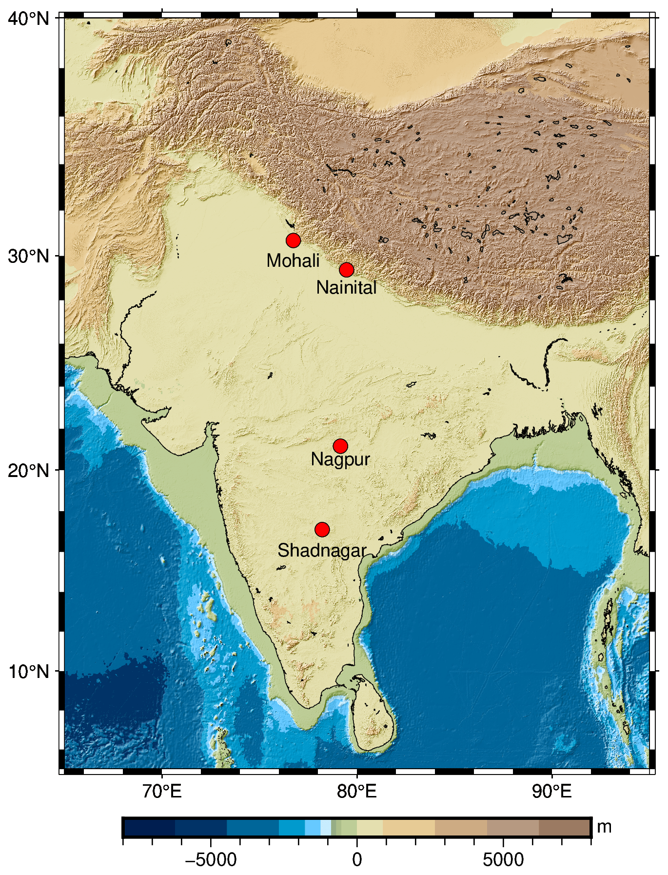
Figure 1Location of CO2 observation sites used in the study.
3.2 Global reanalysis products
We also compared CO2 observations with three global reanalysis products to examine the model–data mismatches at these stations. These products are optimised with available observations of CO2 (e.g. data from surface monitoring stations and total column retrievals from satellites, aircraft missions, ship cruises and AirCore balloon soundings) from different parts of the world. None of these products utilise in situ observations from India. We used atmospheric CO2 concentration from CarbonTracker (CT2019B; Jacobson et al., 2020), CarboScope (s10c_v2020; Rödenbeck et al., 2003; CarboScope, 2020) and ECMWF CAMS (EGG4; Agustí-Panareda et al., 2023; Copernicus Atmosphere Monitoring Service, 2021b) to compare with the observations. All of these reanalysis products differ in their spatial and temporal resolutions. CarbonTracker has a horizontal resolution of 3° × 2° and a temporal resolution of 3 h with 25 vertical levels. CarboScope is a comparatively coarser model with a horizontal resolution of 5° × 3.8° and a temporal resolution of 6 h with 19 vertical levels. Among these products, CAMS EGG4 has the finest spatial resolution at 0.75° × 0.75° in the horizontal direction with 25 vertical levels and a temporal resolution of 3 h. To compare with the observations, simulations from the first vertical level of CarbonTracker are used. Model simulations at a 1000 mbar pressure level from CarboScope and EGG4 are used to compare the observations at the Mohali, Shadnagar and Nagpur stations. Since the Nainital station is a mountain site situated at ∼ 800 mbar height, we compared those observations with CarboScope and EGG4 products at an 800 mbar vertical level.
We have derived different statistical indices to examine the performance of the model simulations to predict the CO2 variability. To quantify the error distribution between the model (P) and observation (O), we have calculated the root mean square error (RMSE) and the mean absolute error (MAE) between the model simulations and observations.
To separate the systematic and unsystematic components from the RMSE, we have used the following method proposed by Willmott (1981). Systematic RMSE is obtained as
and the unsystematic RMSE is obtained as
where .
Here a and b respectively are the intercept and slope of the least-squares regression. The systematic difference for a “perfect” model is expected to be very close to 0, while the unsystematic difference remains close to the value of RMSE. Based on Willmott et al. (2012), we have also computed the refined index of agreement (dr) as follows:
Here, the constant c is set to 2 (Willmott et al., 2012). The dr values can range from −1 to 1. The value indicates the sum of error magnitudes between predicted and observed values relative to the sum of observed deviations around the observed mean. For example, dr=0.5 indicates that the sum of the model–observation mismatch is half the sum of the observed variability around the mean; i.e. dr gives a relative magnitude of the model error compared to the variance of the observations.
5.1 Observed CO2 variability over India
To assess the CO2 variability over India during 2017, we analysed in situ observations of atmospheric CO2 from four different sites (see Sect. 3.1).
Mohali observations show strong variability due to its proximity to urban areas (see Fig. 2a). The Mohali station has hourly observations, and we have separated the daytime values (11:00–16:00 LT) to distinguish the influence of the nocturnal boundary layer on observations (see Fig. 2a). The annual mean of hourly atmospheric CO2 concentration at the Mohali station (whole day) during 2017 is 428.8 ppm with a standard deviation (σ) of 26.6 ppm. For the daytime, the annual mean CO2 is approximately 20 ppm less (408.3 ppm) than all-time value, with a variability (σ) of 11.6 ppm. Since most of the inverse models, which target the retrieval of surface–atmosphere exchange fluxes from in situ observations, use daytime measurements, we carry out the rest of our analysis for Mohali based on daytime values (unless specified otherwise). Monthly mean values of daytime observations show that the Mohali station exhibits strong seasonal variability (σ=9.2 ppm) with approximately a 32.9 ppm difference between maximum and minimum values (see Fig. S7). Maximum intra-month variability is found during January, September, November and December, with a standard variability of 8–12 ppm (Fig. 2a). On a monthly scale, lower values are seen during February (397.9 ppm) and August (391.2 ppm) and higher values are seen during May (413.5 ppm) and November (424 ppm) (Fig. 3a). As expected, the atmospheric CO2 concentration decreases from June onwards due to the enhanced biospheric activity associated with summer monsoon rainfall (Fig. 3a). However, we find high CO2 concentrations at the Mohali station during November, which can be attributed to the agricultural waste-burning activities prominent around this region at this time of the year (Deshpande et al., 2023). A detailed discussion on the influence of biomass burning on CO2 concentration over Mohali is provided in Sect. 6.1. In general, measured CO2 concentration over Mohali shows considerable influences from local fluxes (see Fig. S5).
Mohali observations show strong diurnal variability (σ=14.7 ppm) as well with up to a 40 ppm difference between the maximum and minimum concentrations during the early morning (06:00 LT) and the afternoon (15:00 LT) respectively (Fig. S6). Due to strong mixing, variability in CO2 concentration is less (σ≈12 ppm) during daytime (12:00–15:00 LT) compared to the nocturnal variability of 19–32 ppm (see Fig. S6). A similar reduction in CO2 variability can be seen at 09:00 LT during May–August (Fig. S7), most likely due to a well-established convective boundary layer with strong mixing. Nocturnal CO2 variability during March–May is less compared to other seasons. Apart from this, Mohali observations do not show considerable differences in their diurnal cycle among seasons (Fig. S7).
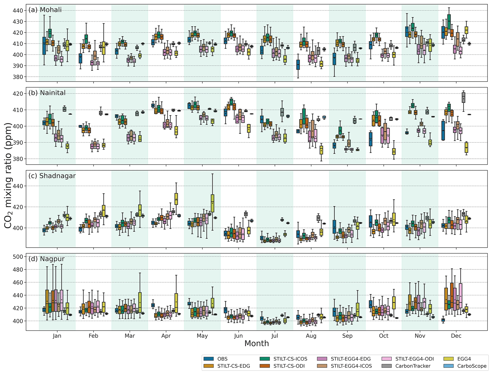
Figure 2CO2 monthly variations over different stations during 2017. Observed CO2 variability is shown in comparison with STILT simulations and global reanalysis products. A box-and-whisker plot of observations in comparison with model simulations is shown. The box denotes the interquartile range, and the whiskers represent the points within 1.5 times the interquartile range from the lower and upper quartile. Additionally, mean values for the CO2 concentration are provided as a black circle inside the box. Daytime (11:00–16:00 LT) values of the Mohali observations and simulations are used.
Monthly mean observations from Nainital also show strong seasonal variations (σ=7.5 ppm) in CO2 concentrations (Fig. 3c) with a difference of up to 25 ppm, between the maximum (412.8 ppm) and minimum (387.9 ppm) concentrations during April and September respectively. Nomura et al. (2021) also reported a similar seasonal cycle over Nainital, with lower values during February–March and September. The observations show an annual mean of 401.6 ppm with a variability reaching 8.4 ppm during 2017. Considerable intra-month variations at the Nainital station are observed during August, October and December with a variability of ∼ 6 ppm (Figs. 2b and S8). In August, CO2 concentrations show a sharp decrease in the concentration of ∼ 18 ppm from previous values at the beginning of the month (∼ 408 ppm; see Fig. 3c).
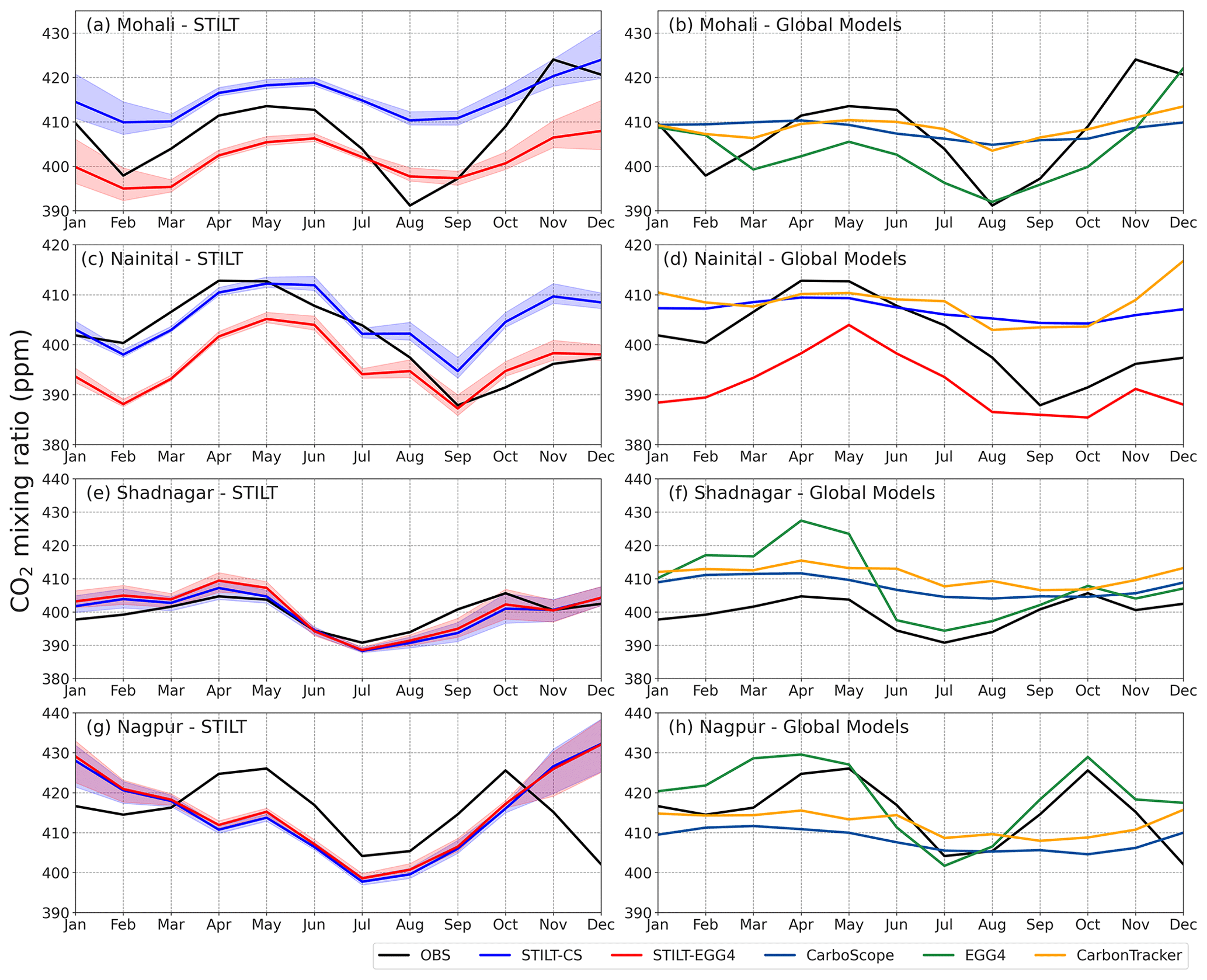
Figure 3CO2 seasonal cycle for different stations. Monthly mean values of CO2 observations in comparison with STILT simulations (a, c, e, g) and global models (b, d, f, h) are given. Blue (STILT-CS) and red (STILT-EGG4) curves represent the ensemble average of the STILT simulations using different anthropogenic fluxes. Shaded regions represent the range of the model simulations.
The annual mean of daily Shadnagar observations was 399.6 ppm during 2017 with a standard deviation of 6.2 ppm (Fig. 2c). At the Shadnagar station, measurements show a seasonal CO2 variability of 4.4 ppm, with two higher peaks during April (404.7 ppm) and October (405.6 ppm), while Sreenivas et al. (2016) reported only one seasonal peak during the pre-monsoon season. The lowest concentration is observed during July (390.8 ppm), with a difference of 14.8 ppm from the highest monthly concentration (Fig. 3e). In general, Shadnagar observations have not shown much intra-month variability (σ ≈ 2 ppm; see Figs.2c and S9) except during the period from August to October (σ ranges from 5.2 to 8.3 ppm). Only daily mean observations from Shadnagar are available for analysis, not hourly data as desired.
The CO2 measurements at the Nagpur station during 2017 show an annual mean of 415.2 ppm, with a variability of 9.5 ppm (Fig. 2d). Nagpur observations show seasonal variability (σ=7.7 ppm) with two maxima and one minimum value with a ∼22 ppm difference between these peaks (Fig. 3g). Enhanced CO2 concentrations are observed during May (426.0 ppm) and October (425.6 ppm). In July, the Nagpur observations show lower concentrations (404.14 ppm) than the rest of the period. A sharp reduction in CO2 concentration (∼ 13 ppm) is found from October to December (see Figs. 3g and S10). Nagpur CO2 observations mostly indicated ∼4 ppm variability within a month (see Figs. 2g and S10), except in June (6.4 ppm), September (9.8 ppm) and October (7.6 ppm). Here we only have access to daily mean observations from Nagpur, not hourly data.
5.2 Comparison between observations and WRF–STILT model simulations
We assessed how well the STILT model simulations agree with observed CO2 variability. For the comparison, we used observations from all four stations described in Sect. 3.1 and a set of six STILT CO2 simulations (see Eq. 5) as described in Sect. 2.
Figure 2a shows the comparison of Mohali daytime observations during 2017 with the STILT simulations. Overall, STILT simulations capture the observed daytime variations reasonably well, with a slight overestimation for STILT-CS simulations and slight underestimation for STILT-EGG4 simulations. Similar to observations, STILT simulations during March–July show less intra-month variability. The maximum variability is found during the winter months. A detailed discussion on the differences in CO2 simulations while using EGG4 and CarboScope as the initial and boundary conditions is provided in Sect. 6.4. STILT simulations with ICOS anthropogenic fluxes showed higher variability (σ≈ 7.3 ppm) than the other simulations.
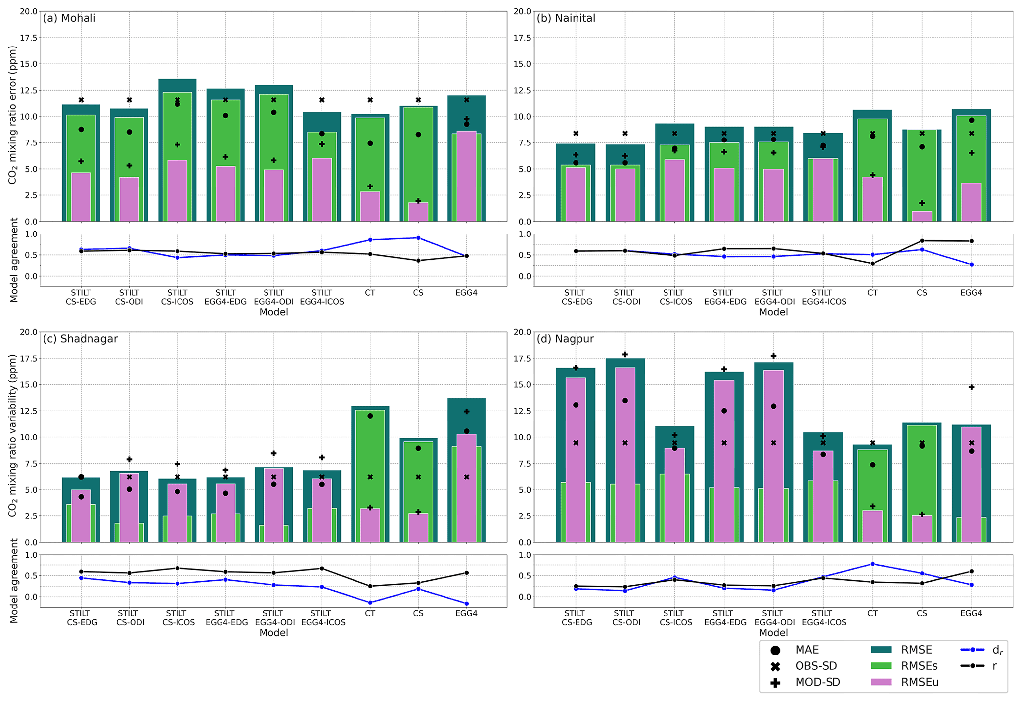
Figure 4An overview of the performances of different models (see Sect. 4). Bar plots represent the different values of RMSE (in teal), systematic RMSE (RMSEs, in lime green) and unsystematic RMSE (RMSEu, in orchid) estimated for each station. MAE (•), observed standard deviation (×) and model standard deviation (+) are overlaid on bar plots. The blue and black lines represent the index-of-agreement (dr) and correlation coefficient (r) values respectively. The panels represent the (a) Mohali, (b) Nainital, (c) Shadnagar and (d) Nagpur stations.
Though STILT simulations capture the seasonal CO2 variability in monthly averaged daytime values over Mohali (see Fig. 3a), the models failed to represent a sharp decline in CO2 concentration during December. The observed decline is likely due to the increased biospheric uptake by rabi crops during this period, which may be misrepresented in the biospheric model. This is further examined in detail in Sect. 6.5. At the same time, monthly averaged values of daytime observations show a second dip in February, which is captured reasonably well by the STILT simulations (Fig. 3a). The simulations could reasonably reproduce the biospheric uptake in August by showing the lowest CO2 concentration in August, similar to observations. The correlation coefficient between monthly averaged observations and STILT simulations varies between 0.86 to 0.89 (STILT-CS) and 0.76 to 0.87 (STILT-EGG4). At a monthly scale, STILT-EGG4 simulations underestimate the seasonal cycle over the Mohali station (RMSE of 6.7–10.0 ppm), while STILT-CS simulations show an overestimation (RMSE of 8.2–11.5 ppm). STILT simulations show an RMSE of 8–9 ppm with the observed intra-seasonal variability in Mohali. The intra-seasonal variability is derived by removing the monthly mean values from the CO2 concentration.
The annually averaged diurnal CO2 concentration shows a good correlation (see Fig. S6) between observation and STILT simulations (0.97–0.99). But there is a significant bias in the STILT-simulated diurnal cycle (see Fig. S6), which is higher for STILT-EGG4 simulations (7.0–18.5 ppm) compared to STILT-CS simulations (5.4–8.2 ppm). The estimated bias is small during summer (MAM) compared to other seasons (Fig. S7). Observations and STILT simulations show less variability during daytime (12:00–18:00 LT) compared to other periods and also have a good model–data agreement during daytime (Fig. S6).
Figure 4 summarises the statistical indices (see Sect. 4) estimated for assessing the model skills. At the Mohali station, STILT CO2 daytime simulations show a standard variability (Fig. 4a) ranging from 5.3–7.3 ppm during 2017, lower than the observed standard variability (11.6 ppm). RMSE for STILT simulations shows a maximum of 13.6 ppm (STILT-CS-ICOS) and a minimum of 10.4 ppm (STILT-EGG4-ICOS). MAE values follow the same pattern as RMSE with reduced magnitude. STILT simulations show a reasonable correlation with observations with coefficient values ranging from 0.53 (STILT-EGG4-EDG) to 0.61 (STILT-CS-ODI). The index of agreement estimated for Mohali varies from 0.44 (STILT-CS-ICOS) to 0.66 (STILT-CS-ODI), indicating that the error values have a magnitude less than or equal to the variability in observations. Analysis of these indices for different months indicates that STILT has a comparatively better prediction capability in summer (March–June) than the rest of the period (figure not shown). The above results show the models' difficulty reproducing mixing during the monsoon season and winter. An inadequate representation of biospheric flux activities in the model can also result in model–observation mismatches. The model skill indices estimated for November are poor owing to the likely misrepresentation of variability associated with biomass burning during these months (Sinha et al., 2014; Pawar et al., 2015).
At the Nainital station, STILT simulations captured the CO2 variability reasonably well, except in the winter period (Figs. 2b and 3c). An offset of 5 ppm is used in STILT-CS simulations at the Nainital station to minimise the consistent overestimation by the model (i.e. 5 ppm is subtracted from the initial CO component). A sharp reduction in observed CO2 concentration from August (Fig. 3c) was not captured by the models (see Sect. 6.5 for a detailed discussion). Noticeably STILT-EGG4 simulations showed an underestimation of CO2 values from January to May. The simulations have a standard deviation of ∼ 6 ppm (6.2–7.1 ppm) in CO2 concentration during 2017, which is lower than the observed standard deviation (Fig. 4b). The RMSE estimated for STILT simulations over Nainital varies between 7.3 to 9.0 ppm. STILT simulations show a reasonable correlation with the observations with a correlation coefficient of ∼ 0.6, except for simulations using ICOS anthropogenic emission fluxes. We get an index of agreement of ∼ 0.5, indicating that the magnitude of STILT model error is half that of the observed variations about the observed mean at the Nainital station. The estimated mismatches for intra-seasonal variability between observation and STILT simulations at the Nainital station is ∼ 4 ppm (based on RMSE).
Comparison of CO2 observations with the model simulations at the Shadnagar station shows that the STILT models can predict the seasonal cycle very well (see Figs. 2c and 3e) with an RMSE of ∼ 4 ppm and correlation ranging from 0.75 to 0.87. Like Nainital, we reduced an offset of 20 ppm in STILT-CS simulations and 5 ppm in STILT-EGG4 simulations to correct the initial CO component. STILT reasonably reproduces the observed intra-month variability except from August to October (Figs. 2c and S9). For Shadnagar, the standard deviation of STILT simulations is higher than the observations (6.2 ppm) and ranges from 6.2 to 8.5 ppm. Estimated RMSE values for STILT simulations are comparatively low at the Shadnagar station and range from 6.2 to 7.2 ppm (Fig. 4c). MAE values vary from 4.3 to 5.5 ppm and follow a pattern similar to that of RMSE. STILT simulations show a reasonable correlation (0.55–0.67) with the observations at the Shadnagar station. But the index of agreement is close to 0 for two simulations (STILT-EGG4-ODI and STILT-EGG4-ICOS), indicating a model error in the simulations as high as observational variability. All STILT simulations show less model skill from August to November. STILT-EGG4 simulations show comparatively less model skill during January–May (figure not shown). The estimated intra-seasonal variability shows an RMSE of 4.3–6.0 ppm with STILT simulations over Shadnagar.
STILT simulations at the Nagpur station capture the observed seasonal variability except for the winter season (Figs. 2d and 3g). The models represent the seasonal cycle from March to October over Nagpur with a correlation coefficient of ∼ 0.97 and RMSE of ∼9 ppm. We reduced an offset of 15 ppm in STILT-CS simulations. The STILT simulations overestimate the winter variability. Also, the intra-month variability at the Nagpur station is overestimated during winter (Figs. 2d and S10). STILT simulations show an RMSE of 6.5–11.5 ppm with the estimated intra-seasonal variations over Nagpur. Notably, the observed decrease in CO2 concentration during the summer monsoon season is well-captured by STILT (Figs. 2d and 3g). However, the increase in the CO2 concentration in STILT simulations during winter months (November–February) is absent in CO2 observations over Nagpur (Fig. 3g). The skill indices for the Nagpur station show that the standard deviation of STILT simulations (10.1–17.9 ppm) is higher than observed standard deviations (Fig. 4d). Also, higher RMSE values (10.5–17.5 ppm) are estimated for STILT simulations at the Nagpur station. Model simulations show very poor correlation coefficient values and index-of-agreement values at the Nagpur region for 2017. We obtained a better model–observation agreement when excluding winter months (November–February). Analysis of model skill indicates that the June–August period has a low RMSE, which can be associated with strong mixing by monsoon winds (figures not shown).
5.3 Comparison between observations and global reanalysis products
We compared observations with three global reanalysis products (CarbonTracker, CarboScope and EGG4) described in Sect. 3.2. The global reanalysis products (except EGG4) could not capture the seasonal variability in CO2 over Mohali (Fig. 3b). The intra-month variability is less in daytime simulations of global models (Fig. 2a) except for EGG4 simulations during winter months (November–February). CarbonTracker and CarboScope show much lower seasonal and intra-seasonal variability over Mohali (Fig. 3b). Global models show an RMSE of ∼ 10 ppm with intra-seasonal variability in observations over Mohali. CarbonTracker exhibits diurnal CO2 variability with a significant underestimation (Fig. S6). EGG4 captured the diurnal variability reasonably well, with a considerable nocturnal bias (Fig. S6). Note that EGG4 has the highest spatial and temporal resolution among the global reanalysis products used in this study. Also, long-range transport has a strong influence on the Mohali site (Pawar et al., 2015), which might contribute to EGG4's better performance. The inter-model differences in intra-month variability are large over Mohali (Fig. 2a), with the standard deviation ranging from 1.9 (CarboScope) to 9.8 ppm (EGG4). The RMSE for global model simulations varies from 10.2–12.0 ppm with correlation coefficients ranging from 0.36–0.52 (Fig. 4a). While we consider the index of agreement, EGG4 shows lower values (0.47) compared to other products, indicating that the magnitude of the error is approximately half of the observed variations.
CarboScope and CarbonTracker also did not capture the seasonal variability in CO2 concentration at the Nainital station. Though it underestimated the variability, EGG4 showed good agreement with the seasonal variations in observations (see Fig. 3d). These reanalysis products show significant differences in CO2 variability with standard deviations varying between 1.8 ppm (CarboScope), 4.4 ppm (CarbonTracker) and 6.9 ppm (EGG4). The observed standard deviation was higher than the standard deviation in these products (Fig. 4b) except for EGG4. EGG4 has the highest RMSE (11.4 ppm) among all products. CarbonTracker also shows a higher RMSE with 10.6 ppm than CarboScope (8.8 ppm). CarboScope and EGG4 models show high correlation values (∼ 0.8) compared to CarbonTracker simulations. EGG4 has a very low index of agreement compared to other model simulations, which indicates that the error in the model simulations is very high compared to the observed variability. A model–observation mismatch of ∼ 5 ppm (RMSE) is observed in the intra-seasonal variability estimated over Nainital.
The standard deviation of EGG4 (12.4 ppm) simulations is higher than the observed standard deviation at the Shadnagar station. But CarbonTracker and CarboScope predicted variability lower than that of the observation (Fig. 4c). EGG4 captures the seasonal cycle over Shadnagar reasonably well but shows high positive bias, reaching up to ∼ 20 ppm during January–May (Fig. 3f). CarbonTracker and CarboScope could not capture the seasonal variability over Shadnagar. The intra-seasonal variability was also poorly represented (Fig. S9) by these products. EGG4 shows the highest RMSE (13.7 ppm) among the global models. The correlation of reanalysis products with Shadnagar observations is low (0.24–0.32) except for EGG4 (0.56) simulations. However, the index of agreement is less than 0 for the EGG4 product, indicating the presence of noise in the simulations. Global models show an RMSE of up to 7 ppm with intra-seasonal variability in observations over Shadnagar.
Among global models, EGG4 shows better agreement with the observations at the Nagpur station, though the variability compared to observations is very high (Fig. 2d). The decline in CO2 concentration during the summer monsoon season is captured by the EGG4 model (Figs. 3h and Fig. S10). EGG4 shows good agreement with the monthly averaged observations at the Nagpur station. But CarbonTracker and CarboScope do not capture the variability in the seasonal cycle well. The standard deviation of EGG4 (14.7 ppm) at the Nagpur station is higher than the observed standard deviation (Fig. 4d). However, the standard deviations of CarboScope (2.7 ppm) and CarbonTracker (3.4 ppm) are lower than the observed standard deviation. The estimated RMSE at the Nagpur station varied from 9.3 to 11.2 ppm. Similar to STILT simulations, global model simulations also show very poor correlation coefficient values at the Nagpur station for 2017. The estimated intra-seasonal variability between global models and observations over Nagpur shows an RMSE of up to 10 ppm.
In the previous sections, we saw that the STILT model has better capabilities than other models in simulating these fine-scale variabilities. Here, we critically examine how well our modelling system can utilise observations from India to deduce optimal information on underlying fluxes at different spatial and temporal scales. The major implications of our results are discussed here, with the interest of further improving the carbon data assimilation over India.
We begin this section by exploring the shortcomings that need to be addressed to use potential CO2 observations from India for inverse optimisation (see Sect. 6.1–6.3). This is because three of the four observation sites used in this study (Mohali, Shadnagar and Nagpur) are situated near cities and are characterised by large intra-seasonal variability. Observations from all these four sites show strong seasonal variations in CO2 concentrations (see Sect. 5.1), contributed by biospheric flux variations and transport mechanisms. Along with the seasonal variations, these observations (except Nainital) are also characterised by strong small-scale variability associated with local flux variations and mesoscale transport processes. It is thus challenging for coarse-resolution models to utilise them for inverse optimisation. Thus, an account of contributions from different sources to the total observed CO2 is discussed in Sect. 6.4, providing useful information about the underlying processes that these observations may carry.
Typically, the highest CO2 concentrations are observed during the April–May period and the lowest values are observed during July–September. The seasonal decrease in CO2 concentration is associated with increased biospheric uptake owing to monsoon rainfall. The seasonal progression of the biospheric uptake across India can also be seen in the observations. That is, observations from the northern part of India (Mohali, Nainital) show the seasonal troughs in CO2 concentrations approximately 1 month after the seasonal troughs at southern Indian stations (Shadnagar, Nagpur). This time lag in ecosystem uptake for northern Indian sites is caused by the monsoon trajectories that result in different arrival times for precipitation across India. Interestingly, Nainital observations indicated a strong biospheric uptake during October–December, which all models (including WRF–STILT) failed to capture. The potential of using Nainital observations via high-resolution inverse modelling to improve the ecosystem uptake and release is further elucidated in Sect. 6.5.
Using the systematic and unsystematic error components in model–data disagreements, Sect. 6.6 discusses the extent to which our model can utilise the full potential of the observations over India, thereby assessing the potential of observations to increase the confidence levels of the derived fluxes.
6.1 Influence of biomass burning on CO2 variability
Agricultural residue burning makes up a major share of biomass burning across India (e.g. Kumar et al., 2011). So, the spatiotemporal extent of biomass fires over India closely follows the area and period of crop harvest. Thus, a greater extent of biomass burning is expected for the pre-monsoon and post-monsoon seasons than for the monsoon season. Considerable aerosols and trace gas emissions are associated with this open agricultural residue burning in the Indo-Gangetic Plain (IGP) and central India (Bhardwaj et al., 2016; Ravindra et al., 2022; Deshpande et al., 2023). For example, the CO2 emission estimated from biomass burning over Punjab (the northern Indian state in which Mohali is located) is 15.62 Mt CO2 yr−1 for the year 2017 (Deshpande et al., 2023). Among the Indian states, Punjab has one of the highest rates of agricultural burning (Sahu et al., 2021; Ravindra et al., 2022; Vellalassery et al., 2021; Deshpande et al., 2023). Consequently, we found a considerable influence of agricultural biomass burning on observations at the Mohali station during November 2017. Many biomass-burning activities were reported in late October and early November 2017 (https://firms.modaps.eosdis.nasa.gov, last access: 14 April 2023). Atmospheric CO2 concentration increased up to 50 ppm, likely in response to the residue burning, with the maximum concentration observed during 5–13 November 2017 (see Figs. S5 and S11b). STILT-derived footprints (Fig. S1 in the Supplement) during November cover the northwestern region of Mohali, indicating the possible influence of biomass burning on the observed variability at the Mohali station. We find a considerable increase in the MODIS-derived fire counts (MODIS-FIRMS, 2021) for October and November 2017 over the Mohali footprint region (see Fig. S11a). A sharp increase in the number of fire occurrences during late October and early November is very likely due to agricultural waste burning after the harvest. We have conducted STILT simulations using biomass-burning fluxes from Global Fire Assimilation System (GFAS) fluxes (Kaiser et al., 2012) and Fire INventory from NCAR (National Center for Atmospheric Research) version 2.5 (FINNv2.5) fluxes (Wiedinmyer and Emmons, 2022; Wiedinmyer et al., 2023). Both of these datasets have a horizontal resolution of 0.1° × 0.1° and a temporal resolution of 1 d. The biomass emission fluxes over the footprint region of Mohali closely follow the fire count data (see Fig. S11a). GFAS emission fluxes over the Mohali footprint region are much less than FINNv2.5 (Fig. S11a). STILT simulations using FINN (STILT–FINN) indicate some influence from biomass burning with a time lead with the CO2 observations (see Fig. S11b). However, STILT simulations using GFAS (STILT–GFAS) could not represent the CO2 contributions from biomass burning (Fig. S11b). The magnitude of CO2 enhancement due to the biomass burning from STILT simulations is 3 ppm, which is ∼ 15 times less than the magnitude of the emission enhancement observed in the CO2 observations (see Fig. S11b). This suggests that the emission inventories need to be improved further to accurately simulate the CO2 variability due to biomass burning in the region. The reanalysis products also failed to capture the variability associated with biomass burning (see Fig. S5). Besides the inaccurate estimation of mixing height, the misrepresentation of emission fluxes, as seen here, can lead to significant errors in the simulated distribution of CO2. This result shows the role of high-resolution fluxes that can account for small-scale events like agricultural waste burning in representing CO2 variability at the Mohali station.
6.2 Influence of emission uncertainties to the CO2 simulations
On estimating terrestrial carbon fluxes, inverse-modelling systems usually assume a known contribution from anthropogenic emissions. However, this assumption would be problematic when utilising observations near urban locations strongly influenced by anthropogenic emissions. For instance, the mean CO component at the Mohali station varies as much as 4 ppm between different emission inventories (EDGAR: 3.1 ppm, ODIAC: 2.5 ppm, ICOS: 7.1 ppm; see Fig. 5). Similarly, an emission contribution difference of up to 5 ppm, as shown by the Shadnagar and Nagpur simulations, also has the potential to bias the inverse flux estimations (Houweling et al., 2010; Schuh et al., 2019). At the same time, Nainital shows the least differences among emission contributions (EDGAR: 1.3 ppm, ODIAC: 1.3 ppm, ICOS: 3.8 ppm), where the above assumption is unlikely to propagate large errors in terrestrial carbon estimations. The choice of emission inventory matters in the regional inverse systems since they may control the majority of CO2 variability when urban sites are utilised. Our results demonstrate large differences among the CO simulations utilising different inventories, indicating the knowledge gap in the emission estimations.
6.3 Sensitivity of simulations to the initial CO2 distribution
STILT prescribes the initial concentration from global models to add the influences from the far-field fluxes to the site simulations. The spatiotemporal details in the prescribed global model can thus influence the STILT CO2 simulations. The differences between the two global reanalysis products used in our STILT simulations caused considerable inter-model mismatches at the Mohali (14 ppm) and Nainital (9 ppm) stations (see Fig. 5, background) while resulting in a negligible bias at the Shadnagar and Nagpur stations. Hence, the uncertainty in representing far-field influences may cause systematic bias in simulated CO2 concentrations, depending on the sites.
6.4 Relative contribution of CO2 components to variability
Here we discuss the contribution from different components, viz. background (CO), biospheric (CO) and anthropogenic (CO) to the total CO2 concentration.
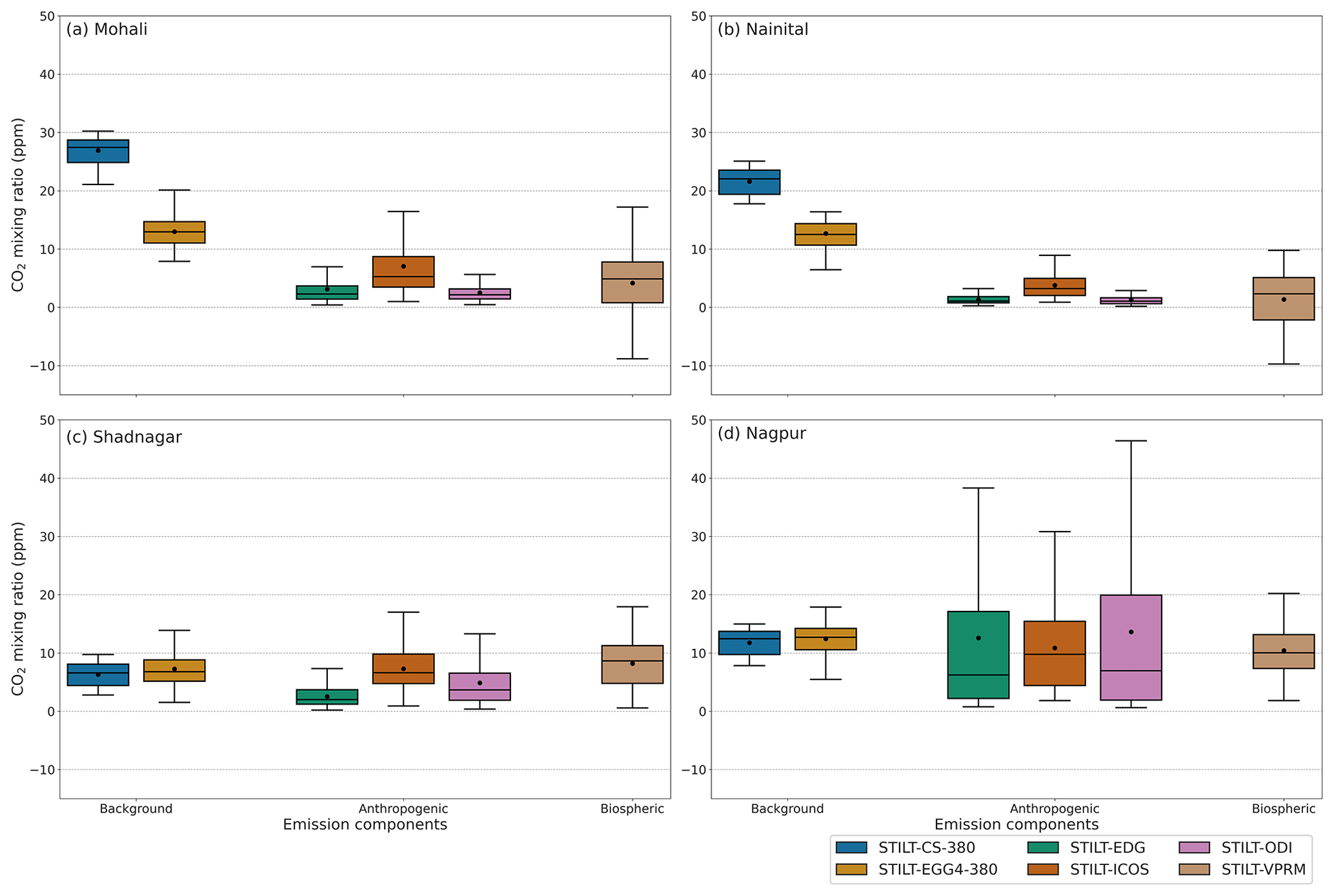
Figure 5Variability in STILT CO2 emission components at different stations. For better comparison with other emission components, 380 ppm is reduced from background components. The box denotes the interquartile range, and the whiskers represent the points within 1.5 times the interquartile range from the lower and upper quartile. Additionally, mean values for the CO2 concentration are provided as a black circle inside the box. The panels represent the variability in (a) Mohali daytime (11:00–16:00 LT) simulations, (b) Nainital, (c) Shadnagar and (d) Nagpur simulations.
The CO2 variability over an observation site is influenced by the flux variability over its footprint region (see Figs. S1–S4). In the context of the inverse modelling that optimises CO2 flux components (such as biospheric, anthropogenic, or both), it is important to ensure a considerable information gain of relevant components when observations from a particular site are utilised. So, here, we investigate the relative contribution of different components to the total CO2 concentration from each observation site. On an annual scale, observations from the Mohali, Shadnagar, and Nagpur sites contain contributions from local fluxes (anthropogenic and biospheric components) by approximately 6 % of the total concentration (see Fig. 5). Regionally advected signals (background component) mostly contribute (99 % of the total) to the Nainital site. CO and CO show almost equal annual contributions in magnitude to the total CO2 concentration in these sites. At the same time, the proportions of contributions to total CO2 can vary with the season, such as winter (DJF) and the pre-monsoon (MAM), monsoon (JJA) and post-monsoon (SON) seasons (figures not shown), due to variations in atmospheric mixing and local fluxes. For instance, the reduction in the CO component over Shadnagar and Nagpur during JJA can very likely be due to increased uptake and mixing during the monsoon period.
There are large differences in local fluxes that drive observed CO2 variability over different sites. Mohali and Nagpur have CO2 variability dominated by anthropogenic activities (σ≈ 5.4 to 13 ppm), while most of the CO2 variability at the Nainital station, situated in the foothills of the Himalayas, is caused by biospheric activities (σ=5.5 ppm) (see Fig. 5). Annually, anthropogenic and biospheric components almost equally contribute to Shadnagar variations (σ≈2.9 to 4.2 ppm).
6.5 Impact of biospheric uptake by crops on CO2 variability
Biospheric fluxes determine CO2 variability at the Nainital station as indicated by the STILT simulated CO component, which shows a seasonal cycle similar to that of the CO2 observations (Fig. S12a). However, the simulated biospheric contribution changes from a negative (sink) to a positive (source) sign during October, while the model significantly overestimates the CO2 concentration (Figs. 3c and S12a). This overestimation corresponds to the misrepresentation of biospheric uptake of about 127 % in the influence region during October–December by VPRM. The improved model's correlation with observations (correlation coefficient of 0.80) and RMSE values (reduced to ∼ 5 ppm) after adjusting the biospheric component (increasing 127 % of biospheric uptake during October–December in the total influence region) increases confidence in simulated transport at the Nainital station (figures not shown). Thus, the above results demonstrate the potential of using Nainital observations via high-resolution inverse modelling to inform about biospheric fluxes.
The variations in CO over Nainital are dominated by crop production (see CO2-NEE_CROP in Fig. S12a; net ecosystem exchange). The variability in the normalised difference vegetation index (NDVI; https://developers.google.com/earth-engine/datasets/catalog/COPERNICUS_S2_SR_HARMONIZED, last access: 25 June 2023) in the footprint region of Nainital, retrieved by the Sentinel-2 MultiSpectral Instrument (MSI) shows a pattern similar to that of the Nainital CO2 observations (see Figs. S2 and S12b). The influence region of the Nainital site covers the entirety of the Indian states of Uttarakhand and Himachal Pradesh and parts of the states of Punjab, Haryana and Uttar Pradesh. The close association of NDVI patterns with the kharif and rabi cropping seasons over the region confirms the enhanced ecosystem uptake due to agricultural activities (Fig. S12b). For example, NDVI increased from July, peaking at the end of August and remaining high until October. The kharif crop cultivation season usually starts in June–July, with a harvesting period from October to November. Further, NDVI increased in December, with another peak in February. Rabi cultivation typically happens around November; these crops are harvested in March–April. The lowest NDVI values for this region are associated with the harvesting period in April–May. Hence, the decrease in CO2 concentration at the Nainital station during August may very likely be due to the strong uptake of kharif crops from the upwind locations of the Nainital station. A slight decrease in Nainital CO2 concentration at the end of December is in response to the biospheric uptake by rabi crops (Umezawa et al., 2016). Nomura et al. (2021) also suggest the influence of cropping patterns over IGP on Nainital observations. Noticeably, the simulated CO2 uptake component (contribution from gross primary production, GPP; see Fig. S12a) from crops shows a pattern similar to that of the Sentinel-2-derived NDVI (see Fig. S12b) in the influence region of Nainital. At the same time, the simulated CO2 component due to the crop's respiration also shows a magnitude of contribution similar that of uptake, nearly neutralising the net biospheric CO2 contribution (Fig. S12a). The overestimation of STILT simulations during October–November over Nainital can thus be due to the considerable overestimation of respiration fluxes or slight underestimation of carbon uptake from crops. Similarly, Mohali observations are influenced by the rabi cultivation in Punjab and IGP, showing a decrease in CO2 concentration during the December–January period, which the models do not represent well. Note that VPRM used in the present study lacks parameter optimisation against eddy-covariance flux observations across India. The availability of eddy-covariance flux observations representing various biomes in India is expected to improve model performance.
6.6 An assessment of the usability of CO2 observations in STILT-based inverse modelling
An accurate estimation of CO2 fluxes through inverse modelling demands proper accountability of CO2 variability by the forward model employed. The disagreements between the observations and simulations largely arise from an inadequate representation of mesoscale transport and local flux influences. Note that the STILT model can represent the seasonal variability at the observational sites (see Sect. 5.2) across India. Since improper accounting of CO2 variability biases the inverse estimations, examining the systematic and unsystematic error terms (decoupled using Eqs. 6 and 7; see Fig. 4) in STILT simulations is particularly relevant to assess the readiness of our models to utilise these measurements in the carbon assimilation system. Though it benefits the inverse-modelling community, this study is not designed to entirely decouple the uncertainties solely due to inadequate transport and improper representation of flux variations in the model.
Figure 4a shows that the Mohali model–observation mismatch is more systematic (66 %–86 %) in nature. High RMSEs values are found over Mohali for most of the cases except for STILT-EGG4-ICOS simulations that utilised EGG4 products as the initial and background condition and ICOS anthropogenic emission fluxes (Fig. 4a). These derived RMSE components and the higher percentage of systematic error contribution suggest further improvements in the models for potentially using Mohali data in inversion. The EGG4 product has a higher spatiotemporal resolution compared to CarboScope, which may contribute to more realistic boundary conditions for the STILT simulation over Mohali. Similarly, the ICOS inventory is the only emission flux used in this study incorporating diurnal, weekly and monthly temporal variations. A reduced RMSEs (66 %) for models using the ICOS inventory suggests a need for representing temporal variations in emission fluxes for improved model performance at the Mohali station, where anthropogenic emissions play a significant role.
The RMSEs for STILT simulations over Nainital varies from 5.4 to 7.6 ppm, constituting about 52 %–60 % of the total RMSE. However, difficulty in capturing decreased CO2 associated with the enhanced biospheric contribution at the Nainital station from August to December (more details in Sect. 6.5) indicates the inadequate representation of ecosystem uptake in the model. For instance, STILT-CS simulations could reproduce the observational variability from January to July with an RMSEs of ∼ 1.5 ppm. Besides the growing period (August to December), the Nainital model–observation mismatch reports only 14 % of the systematic component in the total uncertainty (see Fig. S13). Similarly, the Shadnagar and Nagpur simulations resulted in an RMSEs of 1.6–3.6 ppm (4 %–34 % of total uncertainty) and 5.1–6.5 ppm (8 %–34 % of total uncertainty) respectively. The fact that the majority of the uncertainty in STILT simulations over Nainital, Shadnagar and Nagpur is contributed by unsystematic components shows the ability of the STILT model to represent the CO2 variability there. Hence, these observations can be utilised in inverse optimisation with the help of high-resolution simulations from STILT.
Noteworthy is that the RMSEs values are in general higher for reanalysis products compared to STILT simulations (Fig. 4), resulting in average values of 9.5, 10.4, 7.4 and 11.1 ppm for Nainital, Shadnagar, Nagpur and Mohali respectively. This indicates the advantage of using the STILT model over coarse-resolution models in utilising these observations.
This study examines the potential of a high-resolution WRF–STILT modelling framework to simulate observed CO2 variability over India. Further, we investigate the usability of these observations in inverse modelling when high-resolution models are used. Observations exhibit strong variability at seasonal (7.5–9.2 ppm) and intra-seasonal scales (2–12 ppm). To utilise these observations in inverse optimisations, the models need to address model–observation mismatches arising from fine-scale transport and local flux influences. Our model shows reasonable skill in representing the observed CO2 variability in these stations, though the model could not sufficiently capture all the observed fine-scale variations. By improving fine-scale transport in the model, STILT simulations agree better with the observed seasonal and diurnal variations than the global reanalysis products. Among the reanalysis products, EGG4 products showed reasonable skill in predicting CO2 variability over India.
Further, we explored the limitations of the STILT modelling system in representing the variability, although the model captures the intra-seasonal variabilities much better than the global models. However, the model must account for small-scale flux variations like biomass burning to represent Mohali observations. A considerable portion of these discrepancies can be minimised by improving the prior emission flux distribution at high spatial and temporal scales. Both STILT and global models did not capture the sharp reduction in CO2 concentration at the Nainital station in August, resulting from the increased biospheric uptake by the crops over the IGP region. In addition to using eddy-covariance flux observations in India, utilising additional satellite observations such as solar-induced fluorescence in VPRM can likely improve the prior representation of biospheric CO2 uptake and release across Indian biomes (e.g. Ravi et al., 2023). Further, an improved (inverse) estimate of fluxes can be achieved by utilising atmospheric CO2 observations through carbon data assimilation.
The extent of uncertainties in emission fluxes and their impact on CO2 variations indicate the importance of improving the inventories and their proper representation in atmospheric transport modelling and inverse estimations. For instance, anthropogenic flux variability in CO2 concentration dominates at the Mohali, Shadnagar and Nagpur stations due to their proximity to cities. CO shows significant differences (up to 5 ppm) in their mean values and variability (up to 8 ppm) related to the choice of the emission inventory in the STILT model.
Except for Nainital, the observations used in the study are modulated by influences from local fluxes in addition to background variations. Hence, most of these observations are suitable for constraining carbon fluxes at local-to-urban scales. Nainital observations can be used in the regional carbon estimations as the observations showed significant influences from regional fluxes. Given the availability of high-resolution fluxes and better representation of the fine-scale transport, we demonstrate that STILT can reasonably simulate the CO2 variability over India. In other words, our study demonstrates a possible way of utilising observations from the Indian subcontinent that may potentially improve the estimates of the global assimilation system by increasing the degrees of freedom. Simultaneously, the availability of additional high-frequency observations representing the regional CO2 variability over India, comparable to the World Meteorological Organization standards (https://gml.noaa.gov/ccl/co2_scale.html, last access: 12 June 2023), is necessary for improving the carbon estimates over India at scales relevant to policymaking.
The source code for the WRF model (version 3.9.1.1) that we used for the simulations of the meteorological fields is available at https://www2.mmm.ucar.edu/wrf/users/download/get_source.html (National Center for Atmospheric Research, 2017). The STILT model source code is available at https://stilt-model.org/index.php/FAQ/InitialSetupTasks (Lin et al., 2022). The EGG4 reanalysis products are available at https://doi.org/10.24380/8fck-9w87 (Copernicus Atmosphere Monitoring Service, 2021b). The CarboScope products used in this study are available at https://www.bgc-jena.mpg.de/CarboScope/ (CarboScope, 2020). The CarbonTracker data are available at https://doi.org/10.25925/20201008 (Jacobson et al., 2020). The EDGAR inventory data used in this study are available at https://edgar.jrc.ec.europa.eu/dataset_ghg70 (Crippa et al., 2022). The ODIAC data are available at https://doi.org/10.17595/20170411.001 (Oda and Maksyutov, 2020). The ICOS data are available at https://hdl.handle.net/11676/-XUdi3MSHmJxSVBKmPmrTBOn (Karstens et al., 2019). GFAS data are available at https://ads.atmosphere.copernicus.eu/cdsapp#!/dataset/cams-global-fire-emissions-gfas (Copernicus Atmosphere Monitoring Service, 2021a). The Fire INventory from NCAR (version 2.5) is available at https://doi.org/10.5065/XNPA-AF09 (Wiedinmyer and Emmons, 2022). The Nainital CO2 observations are available at https://doi.org/10.17595/20220301.001 (Terao et al., 2022), and Shadnagar and Nagpur observations are available at https://bhuvan-app3.nrsc.gov.in/data/download/index.php (Bhuvan, 2022). Additional materials, which contain the figures of some analysis for the paper, are available at https://doi.org/10.5281/zenodo.8143361 (Thilakan and Pillai, 2023).
The supplement related to this article is available online at: https://doi.org/10.5194/acp-24-5315-2024-supplement.
DP conceptualised and VT and DP designed the study. VT developed the analysis methods, and VT and JS conducted the model simulations. HH, VS, YT and MN made the CO2 measurements. VT conducted the analyses and wrote the first draft of the manuscript. MVD performed the satellite data acquisition and analysis. DP and CG supported the interpretation of the results. All authors discussed the results and provided feedback on the manuscript.
At least one of the (co-)authors is a member of the editorial board of Atmospheric Chemistry and Physics. The peer-review process was guided by an independent editor, and the author also has no other competing interests to declare.
Publisher’s note: Copernicus Publications remains neutral with regard to jurisdictional claims made in the text, published maps, institutional affiliations, or any other geographical representation in this paper. While Copernicus Publications makes every effort to include appropriate place names, the final responsibility lies with the authors.
Vishnu Thilakan acknowledges the Ministry of Education (MoE) for his PhD funding. We acknowledge the support of IISER Bhopal's high-performance computing facility for STILT model simulations and data analysis. The WRF simulations were done on the high-performance cluster system (Levante) of the German Climate Computing Center (DKRZ). We acknowledge the IISER Mohali Atmospheric Chemistry Facility funded by the Ministry of Education, India, for the data and thank current and previous members of the Atmospheric Chemistry & Emissions Research Group and Aerosol Research Group for technical assistance. The Nainital measurements were supported by the Environment Research and Technology Development Fund (grant nos. JPMEERF20182002 and JPMEERF21S20802) of the Environmental Restoration and Conservation Agency of Japan; the Aryabhatta Research Institute of Observational Sciences (ARIES); and the ISRO Atmospheric Trace gases-Chemistry, Transport and Modelling (AT-CTM) project. We are thankful to Shohei Nomura, Toshinobu Machida, Motoki Sasakawa, Hitoshi Mukai and Deepak Chausali for making the Nainital measurements possible. We thank the Indian Space Research Organisation (ISRO) Geosphere-Biosphere Programme (IGBP) for providing free access to data. We also thank the Bhuvan–National Information System for Climate and Environment Studies (NICES) portal for providing the observations from Shadnagar and Nagpur, as well as Mahesh Pathakoti for technical support. We thank the editor, Abhishek Chatterjee, and referees (Sajeev Philip and the anonymous reviewer) for their constructive involvement in the review process.
This study has been supported by funding from the Max Planck Society allocated to the Max Planck Partner Group at IISER Bhopal.
The article processing charges for this open-access publication were covered by the Max Planck Society.
This paper was edited by Abhishek Chatterjee and reviewed by Sajeev Philip and one anonymous referee.
Agustí-Panareda, A., Diamantakis, M., Massart, S., Chevallier, F., Muñoz-Sabater, J., Barré, J., Curcoll, R., Engelen, R., Langerock, B., Law, R. M., Loh, Z., Morguí, J. A., Parrington, M., Peuch, V.-H., Ramonet, M., Roehl, C., Vermeulen, A. T., Warneke, T., and Wunch, D.: Modelling CO2 weather – why horizontal resolution matters, Atmos. Chem. Phys., 19, 7347–7376, https://doi.org/10.5194/acp-19-7347-2019, 2019. a
Agustí-Panareda, A., Barré, J., Massart, S., Inness, A., Aben, I., Ades, M., Baier, B. C., Balsamo, G., Borsdorff, T., Bousserez, N., Boussetta, S., Buchwitz, M., Cantarello, L., Crevoisier, C., Engelen, R., Eskes, H., Flemming, J., Garrigues, S., Hasekamp, O., Huijnen, V., Jones, L., Kipling, Z., Langerock, B., McNorton, J., Meilhac, N., Noël, S., Parrington, M., Peuch, V.-H., Ramonet, M., Razinger, M., Reuter, M., Ribas, R., Suttie, M., Sweeney, C., Tarniewicz, J., and Wu, L.: Technical note: The CAMS greenhouse gas reanalysis from 2003 to 2020, Atmos. Chem. Phys., 23, 3829–3859, https://doi.org/10.5194/acp-23-3829-2023, 2023. a, b
Bhardwaj, P., Naja, M., Kumar, R., and Chandola, H. C.: Seasonal, interannual, and long-term variabilities in biomass burning activity over South Asia, Environ. Sci. Pollut. Res., 23, 4397–4410, https://doi.org/10.1007/s11356-015-5629-6, 2016. a
Bhuvan: Indian Geo-Platform of ISRO, https://bhuvan-app3.nrsc.gov.in/data/download/index.php, last access: 12 December 2022. a
Boadh, R., Satyanarayana, A., Rama Krishna, T., and Madala, S.: Sensitivity of PBL schemes of the WRF-ARW model in simulating the boundary layer flow parameters for their application to air pollution dispersion modeling over a tropical station, Atmósfera, 29, 61–81, https://doi.org/10.20937/ATM.2016.29.01.05, 2016. a
Broquet, G., Chevallier, F., Bréon, F.-M., Kadygrov, N., Alemanno, M., Apadula, F., Hammer, S., Haszpra, L., Meinhardt, F., Morguí, J. A., Necki, J., Piacentino, S., Ramonet, M., Schmidt, M., Thompson, R. L., Vermeulen, A. T., Yver, C., and Ciais, P.: Regional inversion of CO2 ecosystem fluxes from atmospheric measurements: reliability of the uncertainty estimates, Atmos. Chem. Phys., 13, 9039–9056, https://doi.org/10.5194/acp-13-9039-2013, 2013. a
CarboScope: Jena CarboScope Version s10oc_v2020, Max Planck Institute for Biogeochemistry [data set], http://www.bgc-jena.mpg.de/CarboScope/ (last access: 20 July 2020), 2020. a, b
Chandra, B., Sinha, V., Hakkim, H., and Sinha, B.: Storage stability studies and field application of low cost glass flasks for analyses of thirteen ambient VOCs using proton transfer reaction mass spectrometry, Int. J. Mass Spectro., 419, 11–19, https://doi.org/10.1016/j.ijms.2017.05.008, 2017. a, b
Chandra, N., Lal, S., Venkataramani, S., Patra, P. K., and Sheel, V.: Temporal variations of atmospheric CO2 and CO at Ahmedabad in western India, Atmos. Chem. Phys., 16, 6153–6173, https://doi.org/10.5194/acp-16-6153-2016, 2016. a
Copernicus Atmosphere Monitoring Service: CAMS global biomass burning emissions based on fire radiative power (GFAS), CAMS Atmosphere Data Store (ADS) [data set], https://ads.atmosphere.copernicus.eu/cdsapp#!/dataset/cams-global-fire-emissions-gfas (last access: 10 February 2023), 2021a. a
Copernicus Atmosphere Monitoring Service: CAMS global greenhouse gas reanalysis (EGG4), CAMS Atmosphere Data Store (ADS) [data set], https://doi.org/10.24380/8fck-9w87, 2021b. a, b
Crippa, M., Guizzardi, D., Muntean, M., Schaaf, E., Dentener, F., van Aardenne, J. A., Monni, S., Doering, U., Olivier, J. G. J., Pagliari, V., and Janssens-Maenhout, G.: Gridded emissions of air pollutants for the period 1970–2012 within EDGAR v4.3.2, Earth System Science Data, 10, 1987–2013, https://doi.org/10.5194/essd-10-1987-2018, 2018. a
Crippa, M., Guizzardi, D., Banja, M., Solazzo, E., Muntean, M., Schaaf, E., Pagani, F., Monforti-Ferrario, F., Olivier, J., Quadrelli, R., Risquez Martin, A., Taghavi-Moharamli, P., Grassi, G., Rossi, S., Jacome Felix Oom, D., Branco, A., San-Miguel-Ayanz, J., and Vignati, E.: EDGAR (Emissions Database for Global Atmospheric Research) Community GHG Database (a collaboration between the European Commission, Joint Research Centre (JRC), the International Energy Agency (IEA), and comprising IEA-EDGAR CO2, EDGAR CH4, EDGAR N2O, EDGAR F-GASES version 7.0, European Commission, Joint Research Centre [data set], https://edgar.jrc.ec.europa.eu/dataset_ghg70 (last access: 19 January 2023), 2022. a, b
Deshpande, M. V., Kumar, N., Pillai, D., Krishna, V. V., and Jain, M.: Greenhouse gas emissions from agricultural residue burning have increased by 75% since 2011 across India, Sci. Total Environ., 904, 166944, https://doi.org/10.1016/j.scitotenv.2023.166944, 2023. a, b, c, d
Enting, I. G.: Inverse Problems in Atmospheric Constituent Transport, Cambridge Atmospheric and Space Science Series, Cambridge University Press, https://doi.org/10.1017/CBO9780511535741, 2002. a
Friedlingstein, P., O'Sullivan, M., Jones, M. W., Andrew, R. M., Gregor, L., Hauck, J., Le Quéré, C., Luijkx, I. T., Olsen, A., Peters, G. P., Peters, W., Pongratz, J., Schwingshackl, C., Sitch, S., Canadell, J. G., Ciais, P., Jackson, R. B., Alin, S. R., Alkama, R., Arneth, A., Arora, V. K., Bates, N. R., Becker, M., Bellouin, N., Bittig, H. C., Bopp, L., Chevallier, F., Chini, L. P., Cronin, M., Evans, W., Falk, S., Feely, R. A., Gasser, T., Gehlen, M., Gkritzalis, T., Gloege, L., Grassi, G., Gruber, N., Gürses, Ö., Harris, I., Hefner, M., Houghton, R. A., Hurtt, G. C., Iida, Y., Ilyina, T., Jain, A. K., Jersild, A., Kadono, K., Kato, E., Kennedy, D., Klein Goldewijk, K., Knauer, J., Korsbakken, J. I., Landschützer, P., Lefèvre, N., Lindsay, K., Liu, J., Liu, Z., Marland, G., Mayot, N., McGrath, M. J., Metzl, N., Monacci, N. M., Munro, D. R., Nakaoka, S.-I., Niwa, Y., O'Brien, K., Ono, T., Palmer, P. I., Pan, N., Pierrot, D., Pocock, K., Poulter, B., Resplandy, L., Robertson, E., Rödenbeck, C., Rodriguez, C., Rosan, T. M., Schwinger, J., Séférian, R., Shutler, J. D., Skjelvan, I., Steinhoff, T., Sun, Q., Sutton, A. J., Sweeney, C., Takao, S., Tanhua, T., Tans, P. P., Tian, X., Tian, H., Tilbrook, B., Tsujino, H., Tubiello, F., van der Werf, G. R., Walker, A. P., Wanninkhof, R., Whitehead, C., Willstrand Wranne, A., Wright, R., Yuan, W., Yue, C., Yue, X., Zaehle, S., Zeng, J., and Zheng, B.: Global Carbon Budget 2022, Earth Syst. Sci. Data, 14, 4811–4900, https://doi.org/10.5194/essd-14-4811-2022, 2022. a
Ganesan, A. L., Rigby, M., Lunt, M. F., Parker, R. J., Boesch, H., Goulding, N., Umezawa, T., Zahn, A., Chatterjee, A., Prinn, R. G., Tiwari, Y. K., van der Schoot, M., and Krummel, P. B.: Atmospheric observations show accurate reporting and little growth in India's methane emissions, Nat. Commun., 8, 836, https://doi.org/10.1038/s41467-017-00994-7, 2017. a
Geels, C., Doney, S. C., Dargaville, R., Brandt, J., and Christensen, J. H.: Investigating the sources of synoptic variability in atmospheric CO2 measurements over the Northern Hemisphere continents: a regional model study, Tellus B, 56, 35–50, https://doi.org/10.3402/tellusb.v56i1.16399, 2004. a, b
Geels, C., Gloor, M., Ciais, P., Bousquet, P., Peylin, P., Vermeulen, A. T., Dargaville, R., Aalto, T., Brandt, J., Christensen, J. H., Frohn, L. M., Haszpra, L., Karstens, U., Rödenbeck, C., Ramonet, M., Carboni, G., and Santaguida, R.: Comparing atmospheric transport models for future regional inversions over Europe – Part 1: mapping the atmospheric CO2 signals, Atmos. Chem. Phys., 7, 3461–3479, https://doi.org/10.5194/acp-7-3461-2007, 2007. a
Gerbig, C., Lin, J. C., Wofsy, S. C., Daube, B. C., Andrews, A. E., Stephens, B. B., Bakwin, P. S., and Grainger, C. A.: Toward constraining regional-scale fluxes of CO2 with atmospheric observations over a continent: 2. Analysis of COBRA data using a receptor-oriented framework, J. Geophys. Res.-Atmos., 108, 4757, https://doi.org/10.1029/2003JD003770, 2003. a, b, c, d, e, f
Gerbig, C., Körner, S., and Lin, J. C.: Vertical mixing in atmospheric tracer transport models: error characterization and propagation, Atmos. Chem. Phys., 8, 591–602, https://doi.org/10.5194/acp-8-591-2008, 2008. a
Gerbig, C., Dolman, A. J., and Heimann, M.: On observational and modelling strategies targeted at regional carbon exchange over continents, Biogeosciences, 6, 1949–1959, https://doi.org/10.5194/bg-6-1949-2009, 2009. a
Halder, S., Tiwari, Y. K., Valsala, V., Sijikumar, S., Janardanan, R., and Maksyutov, S.: Benefits of satellite XCO2 and newly proposed atmospheric CO2 observation network over India in constraining regional CO2 fluxes, Sci. Total Environ., 812, 151508, https://doi.org/10.1016/j.scitotenv.2021.151508, 2022. a
Hariprasad, K., Srinivas, C., Singh, A., Vijaya Bhaskara Rao, S., Baskaran, R., and Venkatraman, B.: Numerical simulation and intercomparison of boundary layer structure with different PBL schemes in WRF using experimental observations at a tropical site, Atmos. Res., 145–146, 27–44, https://doi.org/10.1016/j.atmosres.2014.03.023, 2014. a
Hersbach, H., Bell, B., Berrisford, P., Biavati, G., Horányi, A., Muñoz Sabater, J., Nicolas, J., Peubey, C., Radu, R., Rozum, I., Schepers, D., Simmons, A., Soci, C., Dee, D., and Thépaut, J.-N.: ERA5 hourly data on pressure levels from 1979 to present, Copernicus Climate Change Service (C3S) Climate Data Store (CDS) [data set], https://doi.org/10.24381/cds.bd0915c6, 2018a. a
Hersbach, H., Bell, B., Berrisford, P., Biavati, G., Horányi, A., Muñoz Sabater, J., Nicolas, J., Peubey, C., Radu, R., Rozum, I., Schepers, D., Simmons, A., Soci, C., Dee, D., and Thépaut, J.-N.: ERA5 hourly data on single levels from 1979 to present, Copernicus Climate Change Service (C3S) Climate Data Store (CDS) [data set], https://doi.org/10.24381/cds.adbb2d47, 2018b. a
Houweling, S., Aben, I., Breon, F.-M., Chevallier, F., Deutscher, N., Engelen, R., Gerbig, C., Griffith, D., Hungershoefer, K., Macatangay, R., Marshall, J., Notholt, J., Peters, W., and Serrar, S.: The importance of transport model uncertainties for the estimation of CO2 sources and sinks using satellite measurements, Atmos. Chem. Phys., 10, 9981–9992, https://doi.org/10.5194/acp-10-9981-2010, 2010. a
Inness, A., Ades, M., Agustí-Panareda, A., Barré, J., Benedictow, A., Blechschmidt, A.-M., Dominguez, J. J., Engelen, R., Eskes, H., Flemming, J., Huijnen, V., Jones, L., Kipling, Z., Massart, S., Parrington, M., Peuch, V.-H., Razinger, M., Remy, S., Schulz, M., and Suttie, M.: The CAMS reanalysis of atmospheric composition, Atmos. Chem. Phys., 19, 3515–3556, https://doi.org/10.5194/acp-19-3515-2019, 2019. a, b
Jacobson, A. R., Schuldt, K. N., Miller, J. B., Oda, T., Tans, P., Arlyn Andrews, Mund, J., Ott, L., Collatz, G. J., Aalto, T., Afshar, S., Aikin, K., Aoki, S., Apadula, F., Baier, B., Bergamaschi, P., Beyersdorf, A., Biraud, S. C., Bollenbacher, A., Bowling, D., Brailsford, G., Abshire, J. B., Chen, G., Huilin Chen, Lukasz Chmura, Sites Climadat, Colomb, A., Conil, S., Cox, A., Cristofanelli, P., Cuevas, E., Curcoll, R., Sloop, C. D., Davis, K., Wekker, S. D., Delmotte, M., DiGangi, J. P., Dlugokencky, E., Ehleringer, J., Elkins, J. W., Emmenegger, L., Fischer, M. L., Forster, G., Frumau, A., Galkowski, M., Gatti, L. V., Gloor, E., Griffis, T., Hammer, S., Haszpra, L., Hatakka, J., Heliasz, M., Hensen, A., Hermanssen, O., Hintsa, E., Holst, J., Jaffe, D., Karion, A., Kawa, S. R., Keeling, R., Keronen, P., Kolari, P., Kominkova, K., Kort, E., Krummel, P., Kubistin, D., Labuschagne, C., Langenfelds, R., Laurent, O., Laurila, T., Lauvaux, T., Law, B., Lee, J., Lehner, I., Leuenberger, M., Levin, I., Levula, J., Lin, J., Lindauer, M., Loh, Z., Lopez, M., Luijkx, I. T., Myhre, C. L., Machida, T., Mammarella, I., Manca, G., Manning, A., Manning, A., Marek, M. V., Marklund, P., Martin, M. Y., Matsueda, H., McKain, K., Meijer, H., Meinhardt, F., Miles, N., Miller, C. E., Mölder, M., Montzka, S., Moore, F., Josep-Anton Morgui, Morimoto, S., Munger, B., Jaroslaw Necki, Newman, S., Nichol, S., Niwa, Y., O'Doherty, S., Mikaell Ottosson-Löfvenius, Paplawsky, B., Peischl, J., Peltola, O., Jean-Marc Pichon, Piper, S., Plass-Dölmer, C., Ramonet, M., Reyes-Sanchez, E., Richardson, S., Riris, H., Ryerson, T., Saito, K., Sargent, M., Sasakawa, M., Sawa, Y., Say, D., Scheeren, B., Schmidt, M., Schmidt, A., Schumacher, M., Shepson, P., Shook, M., Stanley, K., Steinbacher, M., Stephens, B., Sweeney, C., Thoning, K., Torn, M., Turnbull, J., Tørseth, K., Bulk, P. V. D., Dinther, D. V., Vermeulen, A., Viner, B., Vitkova, G., Walker, S., Weyrauch, D., Wofsy, S., Worthy, D., Dickon Young, and Miroslaw Zimnoch: CarbonTracker CT2019B, NOAA Global Monitoring Laboratory [data set], https://doi.org/10.25925/20201008, 2020. a, b
Jain, C. D., Singh, V., Akhil Raj, S., Madhavan, B., and Ratnam, M. V.: Local emission and long-range transport impacts on the CO, CO2, and CH4 concentrations at a tropical rural site, Atmos. Environ., 254, 118397, https://doi.org/10.1016/j.atmosenv.2021.118397, 2021. a
Janssens-Maenhout, G., Crippa, M., Guizzardi, D., Muntean, M., Schaaf, E., Dentener, F., Bergamaschi, P., Pagliari, V., Olivier, J. G. J., Peters, J. A. H. W., van Aardenne, J. A., Monni, S., Doering, U., Petrescu, A. M. R., Solazzo, E., and Oreggioni, G. D.: EDGAR v4.3.2 Global Atlas of the three major greenhouse gas emissions for the period 1970–2012, Earth Syst. Sci. Data, 11, 959–1002, https://doi.org/10.5194/essd-11-959-2019, 2019. a
Kaiser, J. W., Heil, A., Andreae, M. O., Benedetti, A., Chubarova, N., Jones, L., Morcrette, J.-J., Razinger, M., Schultz, M. G., Suttie, M., and van der Werf, G. R.: Biomass burning emissions estimated with a global fire assimilation system based on observed fire radiative power, Biogeosciences, 9, 527–554, https://doi.org/10.5194/bg-9-527-2012, 2012. a
Karstens, U., Gerbig, C., and Janssens-Maenhout, G.: Global anthropogenic CO2 emissions based on EDGARv4.3 and BP statistics 2019, Carbon Portal [data set], https://hdl.handle.net/11676/-XUdi3MSHmJxSVBKmPmrTBOn (last access: 9 March 2022), 2019. a, b
Kompalli, S. K., Babu, S. S., Moorthy, K. K., Manoj, M., Kumar, N. K., Shaeb, K. H. B., and Joshi, A. K.: Aerosol black carbon characteristics over Central India: Temporal variation and its dependence on mixed layer height, Atmos. Res., 147–148, 27–37, https://doi.org/10.1016/j.atmosres.2014.04.015, 2014. a
Kumar, R., Naja, M., Satheesh, S. K., Ojha, N., Joshi, H., Sarangi, T., Pant, P., Dumka, U. C., Hegde, P., and Venkataramani, S.: Influences of the springtime northern Indian biomass burning over the central Himalayas, J. Geophys. Res.-Atmos., 116, D19302, https://doi.org/10.1029/2010JD015509, 2011. a
Kumar, V. and Sinha, V.: Season-wise analyses of VOCs, hydroxyl radicals and ozone formation chemistry over north-west India reveal isoprene and acetaldehyde as the most potent ozone precursors throughout the year, Chemosphere, 283, 131184, https://doi.org/10.1016/j.chemosphere.2021.131184, 2021. a
Lauvaux, T., Uliasz, M., Sarrat, C., Chevallier, F., Bousquet, P., Lac, C., Davis, K. J., Ciais, P., Denning, A. S., and Rayner, P. J.: Mesoscale inversion: first results from the CERES campaign with synthetic data, Atmos. Chem. Phys., 8, 3459–3471, https://doi.org/10.5194/acp-8-3459-2008, 2008. a
Law, R. M., Rayner, P. J., Steele, L. P., and Enting, I. G.: Using high temporal frequency data for CO2 inversions, Global Biogeochem. Cy., 16, 1-1–1-18, https://doi.org/10.1029/2001GB001593, 2002. a, b
Lin, J. C., Gerbig, C., Wofsy, S. C., Andrews, A. E., Daube, B. C., Davis, K. J., and Grainger, C. A.: A near-field tool for simulating the upstream influence of atmospheric observations: The Stochastic Time-Inverted Lagrangian Transport (STILT) model, J. Geophys. Res.-Atmos., 108, 4493, https://doi.org/10.1029/2002JD003161, 2003. a, b, c, d, e, f
Lin, J. C., Gerbig, C., Wofsy, S. C., Andrews, A. E., Daube, B. C., Grainger, C. A., Stephens, B. B., Bakwin, P. S., and Hollinger, D. Y.: Measuring fluxes of trace gases at regional scales by Lagrangian observations: Application to the CO2 Budget and Rectification Airborne (COBRA) study, J. Geophys. Res.-Atmos., 109, D15304, https://doi.org/10.1029/2004JD004754, 2004. a
Lin, J. C., Gerbig, C., Wofsy, S. C., Andrews, A. E., Daube, B. C., Davis, K. J., and Grainger, C. A.: Stochastic Time-Inverted Lagrangian Transport model, Max Planck Institute for Biogeochemistry [code], Jena, https://stilt-model.org/index.php/FAQ/InitialSetupTasks, last access: 15 March 2022. a
Lin, X., Indira, N. K., Ramonet, M., Delmotte, M., Ciais, P., Bhatt, B. C., Reddy, M. V., Angchuk, D., Balakrishnan, S., Jorphail, S., Dorjai, T., Mahey, T. T., Patnaik, S., Begum, M., Brenninkmeijer, C., Durairaj, S., Kirubagaran, R., Schmidt, M., Swathi, P. S., Vinithkumar, N. V., Yver Kwok, C., and Gaur, V. K.: Long-lived atmospheric trace gases measurements in flask samples from three stations in India, Atmos. Chem. Phys., 15, 9819–9849, https://doi.org/10.5194/acp-15-9819-2015, 2015. a
Mahadevan, P., Wofsy, S. C., Matross, D. M., Xiao, X., Dunn, A. L., Lin, J. C., Gerbig, C., Munger, J. W., Chow, V. Y., and Gottlieb, E. W.: A satellite-based biosphere parameterization for net ecosystem CO2 exchange: Vegetation Photosynthesis and Respiration Model (VPRM), Global Biogeochem. Cy., 22, GB2005, https://doi.org/10.1029/2006GB002735, 2008. a
Mahesh, P., Sreenivas, G., Rao, P., Dadhwal, V., Krishna, S. S., and Mallikarjun, K.: High-precision surface-level CO2 and CH4 using off-axis integrated cavity output spectroscopy (OA-ICOS) over Shadnagar, India, Int. J. Remote Sens., 36, 5754–5765, https://doi.org/10.1080/01431161.2015.1104744, 2015. a, b, c, d
Maier, F., Gerbig, C., Levin, I., Super, I., Marshall, J., and Hammer, S.: Effects of point source emission heights in WRF–STILT: a step towards exploiting nocturnal observations in models, Geosci. Model Dev., 15, 5391–5406, https://doi.org/10.5194/gmd-15-5391-2022, 2022. a
Mathew, T. A., Ravi, A., Pillai, D., Saradambal, L., Kumar, J. S., Gopalakrishnan, M. M., and Thilakan, V.: Evaluating the meteorological transport model ensemble for accounting uncertainties in carbon flux estimation over India, EGUsphere [preprint], https://doi.org/10.5194/egusphere-2023-2334, 2024. a, b
MODIS-FIRMS: MODIS Collection 61 NRT Hotspot/Active Fire Detections MCD14DL distributed from NASA FIRMS [data set], https://doi.org/10.5067/FIRMS/MODIS/MCD14DL.NRT.0061, 2021. a
National Center for Atmospheric Research (NCAR): The Weather Research and Forecasting (WRF) Model, University Corporation for Atmospheric Research [code], https://www2.mmm.ucar.edu/wrf/users/download/get_source.html (last access: 20 January 2022), 2017. a
Nehrkorn, T., Eluszkiewicz, J., Wofsy, S. C., Lin, J. C., Gerbig, C., Longo, M., and Freitas, S.: Coupled weather research and forecasting–stochastic time-inverted lagrangian transport (WRF–STILT) model, Meteorol. Atmos. Phys., 107, 51–64, https://doi.org/10.1007/s00703-010-0068-x, 2010. a, b, c
Nomura, S., Naja, M., Ahmed, M. K., Mukai, H., Terao, Y., Machida, T., Sasakawa, M., and Patra, P. K.: Measurement report: Regional characteristics of seasonal and long-term variations in greenhouse gases at Nainital, India, and Comilla, Bangladesh, Atmos. Chem. Phys., 21, 16427–16452, https://doi.org/10.5194/acp-21-16427-2021, 2021. a, b, c, d, e, f
Oda, T. and Maksyutov, S.: ODIAC Fossil Fuel CO2 Emissions Dataset (Version name : ODIAC2020), Center for Global Environmental Research, National Institute for Environmental Studies [data set], https://doi.org/10.17595/20170411.001, 2020. a, b
Oda, T., Maksyutov, S., and Andres, R. J.: The Open-source Data Inventory for Anthropogenic CO2, version 2016 (ODIAC2016): a global monthly fossil fuel CO2 gridded emissions data product for tracer transport simulations and surface flux inversions, Earth Syst. Sci. Data, 10, 87–107, https://doi.org/10.5194/essd-10-87-2018, 2018. a
Patra, P. K., Canadell, J. G., Houghton, R. A., Piao, S. L., Oh, N.-H., Ciais, P., Manjunath, K. R., Chhabra, A., Wang, T., Bhattacharya, T., Bousquet, P., Hartman, J., Ito, A., Mayorga, E., Niwa, Y., Raymond, P. A., Sarma, V. V. S. S., and Lasco, R.: The carbon budget of South Asia, Biogeosciences, 10, 513–527, https://doi.org/10.5194/bg-10-513-2013, 2013. a
Pawar, H., Garg, S., Kumar, V., Sachan, H., Arya, R., Sarkar, C., Chandra, B. P., and Sinha, B.: Quantifying the contribution of long-range transport to particulate matter (PM) mass loadings at a suburban site in the north-western Indo-Gangetic Plain (NW-IGP), Atmos. Chem. Phys., 15, 9501–9520, https://doi.org/10.5194/acp-15-9501-2015, 2015. a, b, c
Peters, W., Jacobson, A. R., Sweeney, C., Andrews, A. E., Conway, T. J., Masarie, K., Miller, J. B., Bruhwiler, L. M. P., Petron, G., Hirsch, A. I., Worthy, D. E. J., van der Werf, G. R., Randerson, J. T., Wennberg, P. O., Krol, M. C., and Tans, P. P.: An atmospheric perspective on North American carbon dioxide exchange: CarbonTracker, P. Natl. Acad. Sci. USA, 104, 18925–18930, https://doi.org/10.1073/pnas.0708986104, 2007. a, b
Philip, S., Johnson, M. S., Baker, D. F., Basu, S., Tiwari, Y. K., Indira, N. K., Ramonet, M., and Poulter, B.: OCO-2 Satellite-Imposed Constraints on Terrestrial Biospheric CO2 Fluxes Over South Asia, J. Geophys. Res.-Atmos., 127, e2021JD035035, https://doi.org/10.1029/2021JD035035, 2022. a, b
Pillai, D., Gerbig, C., Ahmadov, R., Rödenbeck, C., Kretschmer, R., Koch, T., Thompson, R., Neininger, B., and Lavrié, J. V.: High-resolution simulations of atmospheric CO2 over complex terrain – representing the Ochsenkopf mountain tall tower, Atmos. Chem. Phys., 11, 7445–7464, https://doi.org/10.5194/acp-11-7445-2011, 2011. a
Pillai, D., Buchwitz, M., Gerbig, C., Koch, T., Reuter, M., Bovensmann, H., Marshall, J., and Burrows, J. P.: Tracking city CO2 emissions from space using a high-resolution inverse modelling approach: a case study for Berlin, Germany, Atmos. Chem. Phys., 16, 9591–9610, https://doi.org/10.5194/acp-16-9591-2016, 2016. a
Ravi, A., Pillai, D., Gerbig, C., Sitch, S., Zaehle, S., Thilakan, V., and Jha, C. S.: Spatiotemporal variations in terrestrial biospheric CO2 fluxes of India derived from MODIS, OCO-2 and TROPOMI satellite observations and a diagnostic terrestrial vegetation model, EGUsphere, 2023, 1–69, https://doi.org/10.5194/egusphere-2023-817, 2023. a
Ravindra, K., Singh, T., and Mor, S.: COVID-19 pandemic and sudden rise in crop residue burning in India: issues and prospects for sustainable crop residue management, Environ. Sci. Pollut. Res., 29, 3155–3161, https://doi.org/10.1007/s11356-021-17550-y, 2022. a, b
Rödenbeck, C., Houweling, S., Gloor, M., and Heimann, M.: CO2 flux history 1982–2001 inferred from atmospheric data using a global inversion of atmospheric transport, Atmos. Chem. Phys., 3, 1919–1964, https://doi.org/10.5194/acp-3-1919-2003, 2003. a, b, c, d
Sahu, S. K., Mangaraj, P., Beig, G., Samal, A., Chinmay Pradhan, Dash, S., and Tyagi, B.: Quantifying the high resolution seasonal emission of air pollutants from crop residue burning in India, Environ. Pollut., 286, 117165, https://doi.org/10.1016/j.envpol.2021.117165, 2021. a
Sarangi, T., Naja, M., Ojha, N., Kumar, R., Lal, S., Venkataramani, S., Kumar, A., Sagar, R., and Chandola, H. C.: First simultaneous measurements of ozone, CO, and NOy at a high-altitude regional representative site in the central Himalayas, J. Geophys. Res.-Atmos., 119, 1592–1611, https://doi.org/10.1002/2013JD020631, 2014. a
Schuh, A. E., Jacobson, A. R., Basu, S., Weir, B., Baker, D., Bowman, K., Chevallier, F., Crowell, S., Davis, K. J., Deng, F., Denning, S., Feng, L., Jones, D., Liu, J., and Palmer, P. I.: Quantifying the Impact of Atmospheric Transport Uncertainty on CO2 Surface Flux Estimates, Global Biogeochem. Cy., 33, 484–500, https://doi.org/10.1029/2018GB006086, 2019. a
Shaeb, K. H. B., Rao, K. K., and Althaf, P.: Seasonal Characteristics of Black Carbon Aerosols over an Urban City in India: Source Analysis Using Concentration Weighted Trajectories, Asia-Pacific J. Atmos. Sci., 56, 29–43, https://doi.org/10.1007/s13143-019-00126-9, 2020. a
Sijikumar, S., Raju, A., Valsala, V., Tiwari, Y., Girach, I., Jain, C. D., and Ratnam, M. V.: High-Resolution Bayesian Inversion of Carbon Dioxide Flux Over Peninsular India, Atmos. Environ., 308, 119868, https://doi.org/10.1016/j.atmosenv.2023.119868, 2023. a, b, c
Sinha, V., Kumar, V., and Sarkar, C.: Chemical composition of pre-monsoon air in the Indo-Gangetic Plain measured using a new air quality facility and PTR-MS: high surface ozone and strong influence of biomass burning, Atmos. Chem. Phys., 14, 5921–5941, https://doi.org/10.5194/acp-14-5921-2014, 2014. a, b, c
Sivan, C., Rakesh, V., Abhilash, S., and Mohanakumar, K.: Evaluation of global reanalysis winds and high-resolution regional model outputs with the 205 MHz stratosphere–troposphere wind profiler radar observations, Q. J. Roy. Meteorol. Soc., 147, 2562–2579, https://doi.org/10.1002/qj.4041, 2021. a
Sreenivas, G., Mahesh, P., Subin, J., Kanchana, A. L., Rao, P. V. N., and Dadhwal, V. K.: Influence of Meteorology and interrelationship with greenhouse gases (CO2 and CH4) at a suburban site of India, Atmos. Chem. Phys., 16, 3953–3967, https://doi.org/10.5194/acp-16-3953-2016, 2016. a, b, c
Stein, A. F., Draxler, R. R., Rolph, G. D., Stunder, B. J. B., Cohen, M. D., and Ngan, F.: NOAA’s HYSPLIT Atmospheric Transport and Dispersion Modeling System, B. Am. Meteorol. Soc., 96, 2059–2077, https://doi.org/10.1175/BAMS-D-14-00110.1, 2015. a
Terao, Y., Nomura, S., Mukai, H., Machida, T., Sasakawa, M., and Naja, M.: Atmospheric Carbon Dioxide Dry Air Mole Fraction at Nainital, India, ver.2022.0, NIES [data set], https://doi.org/10.17595/20220301.001, 2022. a, b
Thilakan, V. and Pillai, D.: Additional Materials for “Potential of using CO2 observations over India in regional carbon budget estimation by improving the modelling system”, Version v1, Zenodo, https://doi.org/10.5281/zenodo.8143361, 2023. a
Thilakan, V., Pillai, D., Gerbig, C., Galkowski, M., Ravi, A., and Anna Mathew, T.: Towards monitoring the CO2 source–sink distribution over India via inverse modelling: quantifying the fine-scale spatiotemporal variability in the atmospheric CO2 mole fraction, Atmos. Chem. Phys., 22, 15287–15312, https://doi.org/10.5194/acp-22-15287-2022, 2022. a, b
Thompson, R. L., Ishijima, K., Saikawa, E., Corazza, M., Karstens, U., Patra, P. K., Bergamaschi, P., Chevallier, F., Dlugokencky, E., Prinn, R. G., Weiss, R. F., O'Doherty, S., Fraser, P. J., Steele, L. P., Krummel, P. B., Vermeulen, A., Tohjima, Y., Jordan, A., Haszpra, L., Steinbacher, M., Van der Laan, S., Aalto, T., Meinhardt, F., Popa, M. E., Moncrieff, J., and Bousquet, P.: TransCom N2O model inter-comparison – Part 2: Atmospheric inversion estimates of N2O emissions, Atmos. Chem. Phys., 14, 6177–6194, https://doi.org/10.5194/acp-14-6177-2014, 2014. a
Thompson, R. L., Patra, P. K., Chevallier, F., Maksyutov, S., Law, R. M., Ziehn, T., van der Laan-Luijkx, I. T., Peters, W., Ganshin, A., Zhuravlev, R., Maki, T., Nakamura, T., Shirai, T., Ishizawa, M., Saeki, T., Machida, T., Poulter, B., Canadell, J. G., and Ciais, P.: Top–down assessment of the Asian carbon budget since the mid 1990s, Nat. Commun., 7, 10724, https://doi.org/10.1038/ncomms10724, 2016. a
Tiwari, Y. K., Vellore, R. K., Ravi Kumar, K., van der Schoot, M., and Cho, C.-H.: Influence of monsoons on atmospheric CO2 spatial variability and ground-based monitoring over India, Sci. Total Environ., 490, 570–578, https://doi.org/10.1016/j.scitotenv.2014.05.045, 2014. a
Tolk, L. F., Meesters, A. G. C. A., Dolman, A. J., and Peters, W.: Modelling representation errors of atmospheric CO2 mixing ratios at a regional scale, Atmos. Chem. Phys., 8, 6587–6596, https://doi.org/10.5194/acp-8-6587-2008, 2008. a
Umezawa, T., Niwa, Y., Sawa, Y., Machida, T., and Matsueda, H.: Winter crop CO2 uptake inferred from CONTRAIL measurements over Delhi, India, Geophys. Res. Lett., 43, 11859–11866, https://doi.org/10.1002/2016GL070939, 2016. a
Vellalassery, A., Pillai, D., Marshall, J., Gerbig, C., Buchwitz, M., Schneising, O., and Ravi, A.: Using TROPOspheric Monitoring Instrument (TROPOMI) measurements and Weather Research and Forecasting (WRF) CO modelling to understand the contribution of meteorology and emissions to an extreme air pollution event in India, Atmos. Chem. Phys., 21, 5393–5414, https://doi.org/10.5194/acp-21-5393-2021, 2021. a
Vogelezang, D. H. P. and Holtslag, A. A. M.: Evaluation and model impacts of alternative boundary-layer height formulations, Bound.-Lay. Meteorol., 81, 245–269, https://doi.org/10.1007/BF02430331, 1996. a
Wiedinmyer, C. and Emmons, L.: Fire Inventory from NCAR version 2 Fire Emission, Research Data Archive at the National Center for Atmospheric Research, Computational and Information Systems Laboratory [data set], https://doi.org/10.5065/XNPA-AF09, 2022. a, b
Wiedinmyer, C., Kimura, Y., McDonald-Buller, E. C., Emmons, L. K., Buchholz, R. R., Tang, W., Seto, K., Joseph, M. B., Barsanti, K. C., Carlton, A. G., and Yokelson, R.: The Fire Inventory from NCAR version 2.5: an updated global fire emissions model for climate and chemistry applications, EGUsphere, 2023, 1–45, https://doi.org/10.5194/egusphere-2023-124, 2023. a
Willmott, C. J.: ON THE VALIDATION OF MODELS, Phys. Geogr., 2, 184–194, https://doi.org/10.1080/02723646.1981.10642213, 1981. a
Willmott, C. J., Robeson, S. M., and Matsuura, K.: A refined index of model performance, Int. J. Climatol., 32, 2088–2094, https://doi.org/10.1002/joc.2419, 2012. a, b