Shipping and algae emissions have a major impact on ambient air mixing ratios of non-methane hydrocarbons (NMHCs) and methanethiol on Utö Island in the Baltic Sea

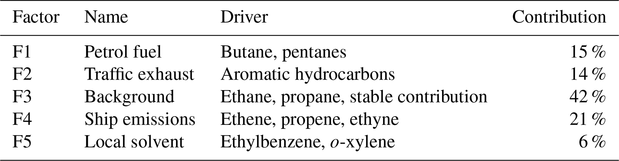
The mixing ratios of highly volatile organic compounds (VOCs) were studied on Utö Island in the Baltic Sea. Measurements of non-methane hydrocarbons (NMHCs) and methanethiol (unexpectedly found during the experiment) were conducted using an in situ thermal desorption–gas chromatography–flame ionization detector/mass spectrometer (TD-GC-FID/MS) from March 2018 until March 2019. The mean mixing ratios of NMHCs (alkanes, alkenes, alkynes, and aromatic hydrocarbons) were at the typical levels for rural/remote sites in Europe, and, as expected, the highest mixing ratios were measured in winter, while in the summertime, the mixing ratios remained close to or below detection limits for most of the studied compounds. Sources of NMHCs during wintertime were studied using positive matrix factorization (PMF) together with wind direction analyses and source area estimates. Shipping was found to be a major local anthropogenic source of NMHCs with a 21 % contribution. It especially contributed to ethene, propene, and ethyne mixing ratios. Other identified sources were petrol fuel (15 %), traffic exhaust (14 %), local solvents (6 %), and long-range-transported background (42 %). Contrary to NMHCs, high mixing ratios of methanethiol were detected in summertime (July mean of 1000 pptv). The mixing ratios followed the variations in seawater temperatures and sea level height and were highest during the daytime. Biogenic phytoplankton or macroalgae emissions were expected to be the main source of methanethiol.

1 Introduction

Atmospheric NMHCs (non-methane hydrocarbons) are composed of light alkanes, alkenes, alkynes, and aromatics with high vapour pressure. Together with compounds containing additional oxygen, sulfur, or other heteroatoms, they are called volatile organic compounds (VOCs). NMHCs are emitted to the atmosphere due to fossil fuel or wood burning, solvent usage, gas leakage, etc. (e.g. Ge et al., 2024). Some VOCs (e.g. isoprene and monoterpenes) are mainly emitted from biogenic sources (Guenther et al., 2012). In the atmosphere, NMHCs react with nitrogen oxides by means of hydroxyl (OH) radical reactions, leading to the production of ozone. Ozone is a phytotoxic compound that is also harmful to health. Therefore, the European Union has set limit values for ozone concentrations and implements policies to reduce emissions of ozone precursors. During the period 1994–2020, the emissions of NMHC in the European Union decreased by ∼ 58 % (EMEP, 2023).

While NMHC mixing ratios have already been monitored for decades at several locations in Europe and their emissions are reported to the databases (e.g. EMEP, 2023; Ge et al., 2024), less is known about the marine areas and impacts of shipping on NMHCs mixing ratios. Together with other pollutants (e.g. particles, sulfur dioxide, and nitrogen oxides), combustion in ship engines produces NMHCs, and these emissions may have strong impacts on the air quality in coastal and marine areas (e.g. Viana et al., 2014; Tang et al., 2020).

In northern Europe, the source areas of NHMCs have been studied earlier at the sub-Arctic site of Pallas, Finland (Hellén et al., 2015), where source area studies of NMHCs indicated that the EU was no longer a significant source area for NMHCs at that study site. The main source area was in eastern Europe, to the south-east of Pallas. However, source apportionment was not studied. Positive matrix factorization (PMF) is a commonly used method in source apportionment studies of air pollutants (Sun et al., 2020). It has also been applied to NMHCs at different kinds of locations, but only a few studies have used it on NMHCs at remote/rural sites (Leuchner et al., 2015; Lanz et al., 2009; Sauvage et al., 2009). Vestenius et al. (2021) applied PMF to more reactive biogenic VOCs in a boreal forest. In these kinds of environments, photochemical ageing must be considered when interpreting the results (Yuan et al., 2012).

Missing OH reactivity (up to 3.5 s⁻¹) found in oceanic regions worldwide clearly indicates that there is also a significant amount of additional currently unidentified reactive compounds emitted in marine areas (Thames et al., 2020). Fluctuations in missing reactivity correlate with dimethylsulfide (DMS) and sea surface temperature. DMS is known to be emitted by marine biota, but less is known about other sulfuric compounds (Yu and Li, 2021). In the atmosphere, organic sulfur compounds undergo oxidation to form sulfur dioxide (SO₂), which is further oxidized to produce sulfuric acid and sulfate aerosols. These aerosols influence cloud radiative properties, impacting the climate (Hopkins et al., 2023). In coastal areas, sulfur compounds may also impact air quality. Better knowledge about the marine sulfuric emissions is also essential for evaluating the consequences of reduced SO₂ emissions from shipping. While lower emissions are anticipated to enhance air quality, there is a possibility of adverse effects on climate (Sofiev et al., 2018).

One of the potential candidates to explain this discrepancy is methanethiol. Due to its high reactivity with OH radicals, it is a promising candidate for the missing reactivity found in marine areas. Methanethiol is known to be emitted from phytoplankton, but the factors that control its production and emission rates are not well understood (Kilgour et al., 2022; Novak et al., 2022). It is formed in the seawater from the same precursor metabolite, dimethylsulfoniopropionate (DMSP), as DMS (Kiene and Linn, 2000). In addition to phytoplankton, Cyanobacteria are also noted as a source of methanethiol (Watson and Jüttner, 2017). In the atmosphere, methanethiol oxidizes with hydroxyl (OH) radicals 7 times faster than DMS (Kilgour et al., 2022), and OH oxidation of methanethiol produces SO₂ with almost unity yield (Novak et al., 2022). There is very little information on atmospheric mixing ratios of methanethiol. Lawson et al. (2020) and Novak et al. (2022) measured mean mixing ratios of ∼ 20 pptv in the south-western Pacific Ocean and at the Scripps Institution of Oceanography in La Jolla, CA, USA, respectively. Due to the high reactivity of the methanethiol, its mixing ratios are expected to remain low, even with relatively high emissions, and, therefore, VOC monitoring networks with marine stations (e.g. the Global Atmospheric Watch programme and the Aerosol, Clouds and Trace Gases Research Infrastructure, ACTRIS) may have overlooked it. Even with a mean mixing ratio of ∼ 20 pptv, Novak et al. (2022) estimated that methanethiol could be a source of up to 30 % of the SO₂ formed in the marine boundary layer in coastal California.

The aim of this study was to characterize the most volatile organic compounds in more detail in marine air in the Baltic Sea. Since terrestrial anthropogenic sources of NMHCs are relatively well known, we focused on quantifying the impact of shipping on their mixing ratios. NMHCs containing two to nine carbon atoms were measured at the same location on Utö Island in the Baltic Sea as in our previous studies (Laurila and Hakola, 1996; Hakola et al., 2006). In these earlier studies, air samples were systematically collected twice a week using stainless-steel canisters followed by detailed laboratory analysis. Now, with in situ measurements and a higher (2 h) time resolution, it was possible to study source apportionment and source areas of measured NMHCs in more detail and to use PMF combined with wind direction distributions and source area analyses. Given the high reactivity observed in marine areas, which cannot be attributed to currently known anthropogenic or biogenic compounds (Thames et al., 2020), our objective was also to explore and identify novel compounds. During the measurements, we detected an additional peak, which was identified as methanethiol. Results concerning methanethiol mixing ratios and its possible sources are presented to show the need for more studies on this compound.

2 Experimental setups

2.1 Measurement site

The Utö Atmospheric and Marine Research Station of the Finnish Meteorological Institute (59°46^′50 N, 21°22^′23 E) is located at the outermost edge of the Archipelago Sea, facing the Baltic Sea. The station provides an excellent possibility for observing marine biogenic emissions with minimal interference from terrestrial sources. The station produces real-time, high-frequency measurements of the physical, chemical, and biological features of the water column and atmospheric concentrations of trace gases and aerosols (Fig. 1a; Laakso et al., 2018; Kraft et al., 2021; Honkanen et al., 2018, 2021, 2024; Rautiainen et al., 2023).

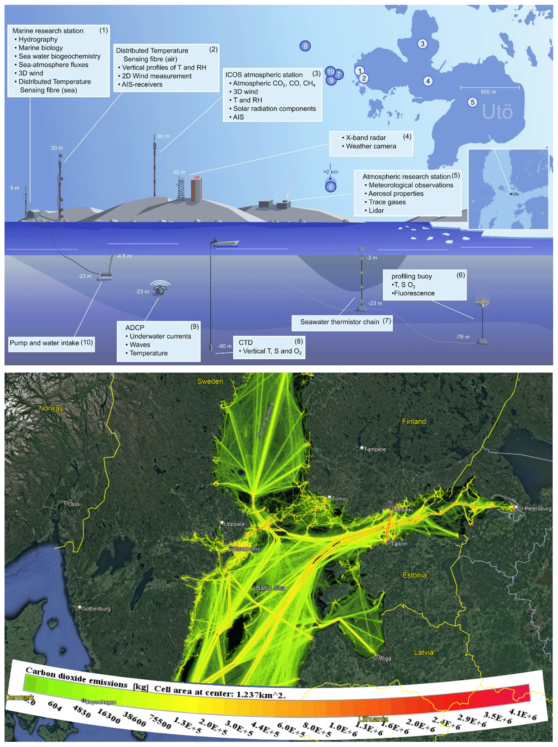
Figure 1 (a) Description of the Utö marine research station and (b) predicted CO₂ emissions from ships sailing the Baltic Sea during 2022 (map © 2023 Google; image by Landsat/Copernicus). The main shipping routes are coloured according to emissions in relative mass units per unit area.

2.2 Measurements of NMHCs and methanethiol

The samples were collected from a 9 m long mast (inlet of 12 m a.s.l.; Fig. 1; Marine research station 1) with a flow rate of ∼ 2.2 L min⁻¹. The mast is located approximately 5 m from the sea on the western edge of Utö Island. A subsample was collected in a gas chromatograph through a heated line. An in situ thermal desorption unit (Unity 2 + Air Server 2; Markes International Ltd.) connected to a gas chromatograph (Agilent 7890) with a mass spectrometer (Agilent 5975C) and a flame ionization detector (TD-GC-FID/MS) was used. Two columns (HP-1 with the dimensions 50 m × 0.22 mm × 1 µ m and Al/Na₂SO₄ PLOT with the dimensions 50 m × 0.32 mm) were connected using an Agilent Deans switch. Samples were taken every other hour from a 35 m long fluorinated ethylene propylene (FEP) inlet ($\mathrm{1}/\mathrm{8}$ in. i.d.) located on the 9 m long mast. An extra flow of 2.2 L min⁻¹ was used to avoid losses of the compounds on the walls of the inlet tube. Samples were collected directly from this ambient airflow through a Nafion dryer into the cold trap (U-T17O3P-2S; Markes International Ltd.) of the thermal desorption unit. The sampling time was 30 min, and the sampling flow through the cold trap was 20 mL min⁻¹. All the lines and valves in the thermal desorption unit were kept at 200 °C. During sampling, the cold trap was kept at −30 °C. For desorption, the cold trap was heated to 300 °C for 3 min and flushed with a helium flow of 10 mL min⁻¹. Every 50th sample was a calibration sample. The calibration gas (National Physical Laboratory; 30 VOC mix) contained C₂–C₈ alkanes, C₂–C₅ alkenes, C₆–C₉ aromatic hydrocarbons, ethyne, and isoprene at a ∼ 4 ppb level. Compounds detected and quantified were ethane, ethene, ethyne, propane, propene, n-butane, i-butane, n-pentane, i-pentane, 2-methylpentane, benzene, toluene, ethylbenzene, o-xylene, p/m-xylene, and methanethiol. Mixing ratios of the other NMHCs in the calibration gas remained below detection limits.

In spring and summer, we detected an unknown compound on the flame ionization detector. It was later identified as methanethiol. Methanethiol was not included in the standard mixture used, but it was later identified based on an authentic standard (Linde gas/BOC; five-component mix at a 10 ppm level) and it was also detected from Cyanobacteria culture samples grown in the laboratory. It was calibrated as close-eluting pentane and corrected based on carbon number.

2.3 Positive matrix factorization (PMF) modelling

The Utö winter NMHC dataset was analysed using the United States Environmental Protection Agency's positive matrix factorization (EPA PMF) model version 5.0. PMF (positive matrix factorization) is a receptor modelling tool that is widely used in source apportionment of air pollution (Hopke, 2016; Hopke et al., 2020). PMF decomposes the measured time series data matrix into two matrices (i.e. factor contributions and factor profiles) and then uses a chemical mass balance equation to find a number of user-specified factors (potential sources) that affect the measured species' concentration at the receptor. The results are constrained to non-negativity for the factor profiles and non-significant negativity for the factor contributions. VOC concentrations and especially biogenic VOC emission profiles may change quite rapidly in the atmosphere on the way from emissions to the receptor site due to the high reactivity of VOCs. Prior works on the source apportionment of biogenic VOCs have shown that PMF is also a valuable tool for these kinds of data (e.g. Vestenius et al., 2021). Even though studied anthropogenic NMHCs have longer atmospheric lifetimes than those of biogenic VOCs, their ratios may still vary during the transport, and this has to be taken into account when interpreting the results.

All compounds quantified except p/m-xylene and methanethiol were used for the PMF analyses. Methanethiol remained below the detection limit during the winter months and p/m-xylene comprised < 2 % of the total detected VOC mixing ratio. Uncertainty calculations for the PMF model were made according to Polissar et al. (1998). The expanded measurement uncertainty (U) was estimated from partial uncertainties in analytical precision, standard preparation, and sampling flow. As PMF does not tolerate missing values in the data matrix, missing values (e.g. missing species in the sample) were replaced by the species median with their uncertainties multiplied by 10 so that these “synthetic” data would not have an effect on the model resolution. Values below the limit of detection (< LOD) were replaced by 0.5 ⋅ LOD and their respective uncertainties were set to $\mathrm{5}/\mathrm{6}$ ⋅ LOD. Species were categorized as “strong”, “weak”, or “bad” using their sample-to-noise ($\mathrm{S}/\mathrm{N}$) ratios. Species with $\mathrm{S}/\mathrm{N}$ ratios over 2 were generally categorized as strong, and species with $\mathrm{S}/\mathrm{N}$ values between 0.2 and 2 were generally categorized as weak. Species with $\mathrm{S}/\mathrm{N}$ values lower than 0.2 were categorized as bad and were removed from the model. Weak categorization increases the species' uncertainty by a factor of 3. However, only 3 of the 14 modelled species (ethane, ethylbenzene, and toluene) were categorized as strong; the other 11 species were categorized as weak due to their low $\mathrm{S}/\mathrm{N}$ ratio. Uncertainty analyses of the model results were made using bootstrapping. The factor contributions (time series) were combined with local wind data using the openair software package in R (Carslaw, 2018). A conditional bivariate probability function (CBPF) was used to estimate the conditional probabilities of source directions and distance from the receptor using local wind measurements. The CBPF takes wind speed into account as a third variable in addition to concentration and wind direction and gives the probability of direction and the likely distance of high factor contributions (potential source). In the CBPF, the 75th percentile was used as the threshold value; therefore, the analysis gives the probability of direction and the likely distance of the highest factor contributions.

2.4 Source area estimates

Adjoint atmospheric dispersion simulations were used to identify the source areas for the samples collected during the measurements. The method is quite similar to the one used by Meinander et al. (2013), Hellén et al. (2015), and Meinander et al. (2020), but for the sake of completeness, we briefly describe it below.

The simulations were performed with SILAM v5.8 (System for Integrated Modeling of Atmospheric Composition; http://silam.fmi.fi; last access: 21 August 2023). This system incorporates an Eulerian non-diffusive transport scheme (Sofiev et al., 2015). The model has been extensively validated for a variety of atmospheric dispersion and source inversion problems on a regional and global scale (Petersen et al., 2019; Kouznetsov et al., 2020).

The model was driven with the meteorological fields from ERA-5 (Hersbach et al., 2020) at a resolution of 0.25 × 0.25°. Adjoint simulations were performed on a 0.5° × 0.5° resolution grid, with eight vertical layers of varying thicknesses, spanning from 30 m at the surface to 2000 m at altitudes of up to 6 km. For each of the about 900 samples collected, the model was integrated for 6 d backwards in time on a domain covering northern Europe. The resulting fields of sensitivity distribution (also known as footprints or retroplumes) were aggregated in time and stored for further analysis.

Each measured sample combines contributions from spatially and temporally distributed sources. Adjoint simulations allow for reconstructing a 4D sensitivity pattern of each sample to the location of a source in space and time. Combining the sensitivities with the sampled values, one can infer the likely source areas for a specific variable. Since the individual observed compounds are highly correlated in the samples in this study, we used the concentrations of the PMF factors rather than concentrations of individual compounds. For each of the factors, the retroplumes were aggregated for below the 20th percentile and above the 80th percentile to get typical “clean-sample” source areas and “polluted-sample” source areas. The aggregated retroplumes show the relative sensitivity of the corresponding samples to various locations of the emission source. The areas that are high for polluted samples but low for clean ones are likely the origin of the specific factor.

2.5 Complementary data

Total phytoplankton biomass was obtained using imaging flow cytometry. An Imaging FlowCytobot (IFCB; McLane Research Laboratories, Inc., USA) was connected to the Utö station's flow-through system and took a 5 mL sample approximately every 20 min. A chlorophyll a trigger was used to target the phytoplankton community (detailed explanation of the sampling system can be found in Kraft et al., 2021). The data were classified using a convolutional neural network classifier and image-specific biovolumes were computed (Moberg and Sosik, 2012; Kraft et al., 2022). The total phytoplankton biomass was calculated by summing up the total biovolumes of all classes, also including unclassified images, and converting the total biovolume (µm³ mL⁻¹) to total biomass (µg L⁻¹) by assuming a plasma density of 1 g cm⁻³ (CEN, 2015).

The used meteorological data and ozone (O₃), sulfur dioxide (SO₂), particulate matter < 2.5 µm (PM_2.5), and nitrogen dioxide (NO₂) concentration data are available at the Finnish Meteorological Institute open-access data portal (https://en.ilmatieteenlaitos.fi/download-observations; last access: 21 June 2023). The data were collected at a nearby atmospheric research station on Utö Island (Fig. 1a). Temperature and wind speed and direction were measured by the automatic weather station. The concentration of NO₂ was measured by a Thermo Electron 42i-TL analyser, O₃ by an ambient air O₃ monitor (TEI 49i), SO₂ by a Thermo Electron 43i TLE analyser, and PM_2.5 by a Thermo 5030 SHARP analyser, all produced by Thermo Fischer Scientific, Waltham, USA.

Sea surface temperature was measured at a wave buoy 60 km to the south-west of Utö with a Datawell DWR4 Waverider buoy. Sea level height at Utö was interpolated from tide gauge observations at Föglö (62 km from Utö) and Hanko (90 km from Utö). The values are given relative to the theoretical mean sea level.

Carbon dioxide (CO₂) emissions originating from ship traffic over the Baltic Sea were used for presenting main shipping routes (Fig. 1b). The emissions were modelled using the Ship Traffic Emission Assessment Model (STEAM), which uses automatic identification system data to describe ship traffic activity. The method is presented elsewhere (Jalkanen et al., 2009, 2012; Johansson et al., 2017).

3 Results and discussion

3.1 Mixing ratios of NMHCs

The mean mixing ratios were at typical levels for rural/remote sites in Europe (Solberg et al., 2020). Ethane and propane were clearly the most abundant NMHCs detected, contributing mean percentages of 43 % and 15 %, respectively, to the total NMHC mixing ratio. The mean contribution of aromatic hydrocarbons (benzene, toluene, ethylbenzene, and xylenes) was only 8 %. The seasonal variations in NMHCs followed a well-known cycle with maximum mixing ratios during the dark wintertime and minimum mixing ratios during summer, when mixing ratios of many compounds were below detection limits due to effective sink reactions with OH radicals (Fig. 2). Generally, the more reactive the compounds, the larger the amplitude between summer and winter mixing ratios. NMHCs were measured on Utö Island in the Baltic Sea in Finland during 1992–2007 by collecting air samples in stainless-steel canisters twice a week for further analysis in the laboratory (Laurila and Hakola, 1996; Hakola et al., 2006). These studies also found a clear seasonal cycle of the NMHCs, with the highest mixing ratios during winter. The seasonal cycle of methanethiol is contrary to the other VOCs as expected, since it is of biogenic origin and not emitted in wintertime.

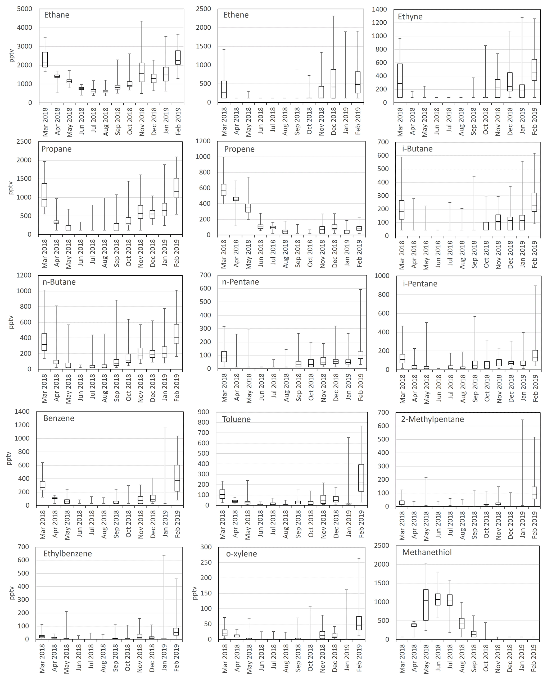
Figure 2 Monthly-mean box and whisker plots of measured mixing ratios (pptv). The boxes represent second and third quartiles, and the vertical lines in the boxes represent median values. The whiskers show the highest and the lowest measurements. The number of data points for each compound was 2175–2188. Values < LOD were marked as 0.5 ⋅ LOD.

3.2 Source apportionment of NMHCs

In PMF modelling, different combinations of solutions with four to seven source factors were tested. The most reasonable and interpretable results were obtained by a five-factor solution, which was chosen for further investigation. Also, bootstrapping showed acceptable results to all factors for this solution, with no swaps for factors F1 to F4 and 95 % mapping for F5, which is well within the acceptable range (80 %). One of the factors represents regional background air and the other four factors were interpreted as the local solvent and ship, petrol, and traffic exhaust emissions as represented in Table 1 and described below. For PMF analysis, we could only use winter data since the mixing ratios of many of the compounds were very low or below detection limits during other times. The profiles of factors are not expected to directly represent the profiles of real emissions since most of these emissions are transported to the site over long distances, and during transportation, NMHCs are oxidized with different rates, which means that the ratios of the compounds may change. This has been considered when interpreting the results. Ethane has a relatively high contribution to all factors (Fig. 3a). Ethane is the longest-living NMHC in the atmosphere and has the highest mixing ratios. The background factor (F3) is a major contribution factor for ethane (Fig. 3b). Due to the high mixing ratios of ethane compared to other compounds (Fig. 2), small changes in ethane mixing ratios (even within uncertainties) may result in high contributions to the other factors. This has also been considered when interpreting the results.

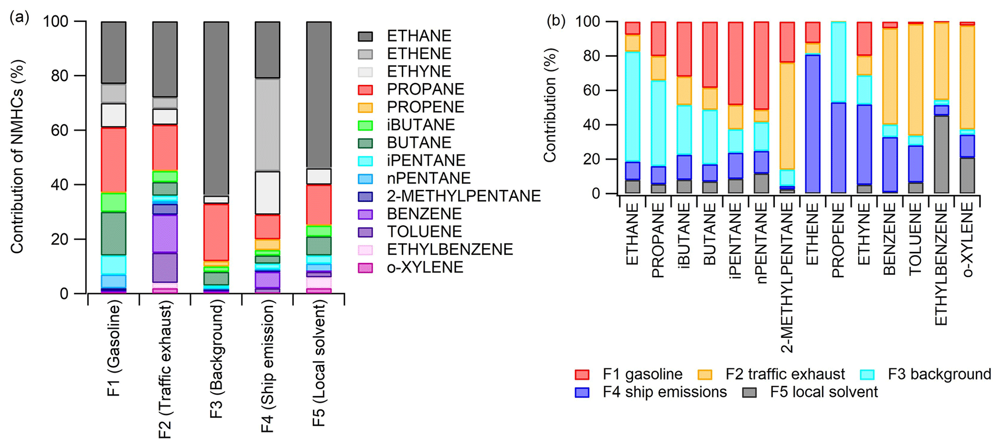
Figure 3 (a) Relative contributions of the compounds' mixing ratios in factors (% of factor sum) and (b) relative contribution of the factors on the average compound mixing ratios for the period of observations.

3.2.1 Identification of the PMF factors

Factor 1 (F1) was identified as petrol fuel emissions (gasoline in Figs. 4 and 5). The factor had a high contribution to butanes and pentanes (Fig. 3). These compounds are known to make a major contribution to the NMHC emissions of petrol fuel and especially evaporated petrol (Hellén et al., 2006). Wind direction distribution indicated that the main source for this factor was further away to the east of the measuring site (Fig. 4). This direction includes the main harbours in the Gulf of Finland and the city of Saint Petersburg. This is supported by the sensitivity maps (Fig. 5). The maps corresponding to the clean samples for F1 (petrol) have clear gaps over Russia and the southern shore of the Gulf of Finland, which correspond to high values in the polluted maps (Fig. 5a and b). These areas likely contribute to high concentrations of this factor.

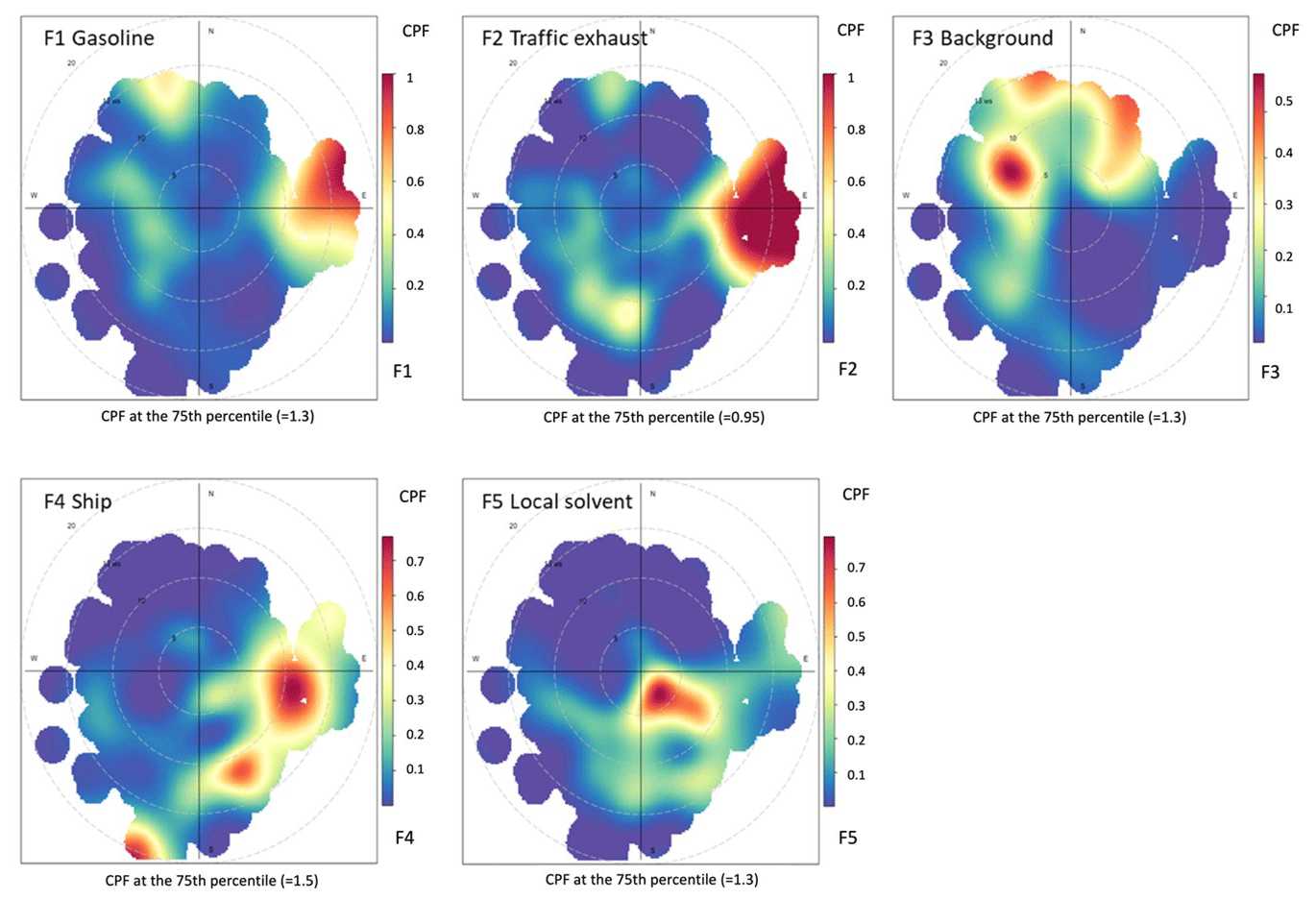
Figure 4 Probability function of distribution of wind direction and speed corresponding to the PMF factors. Dashed circles show the wind speed in 5 m s⁻¹ increments.

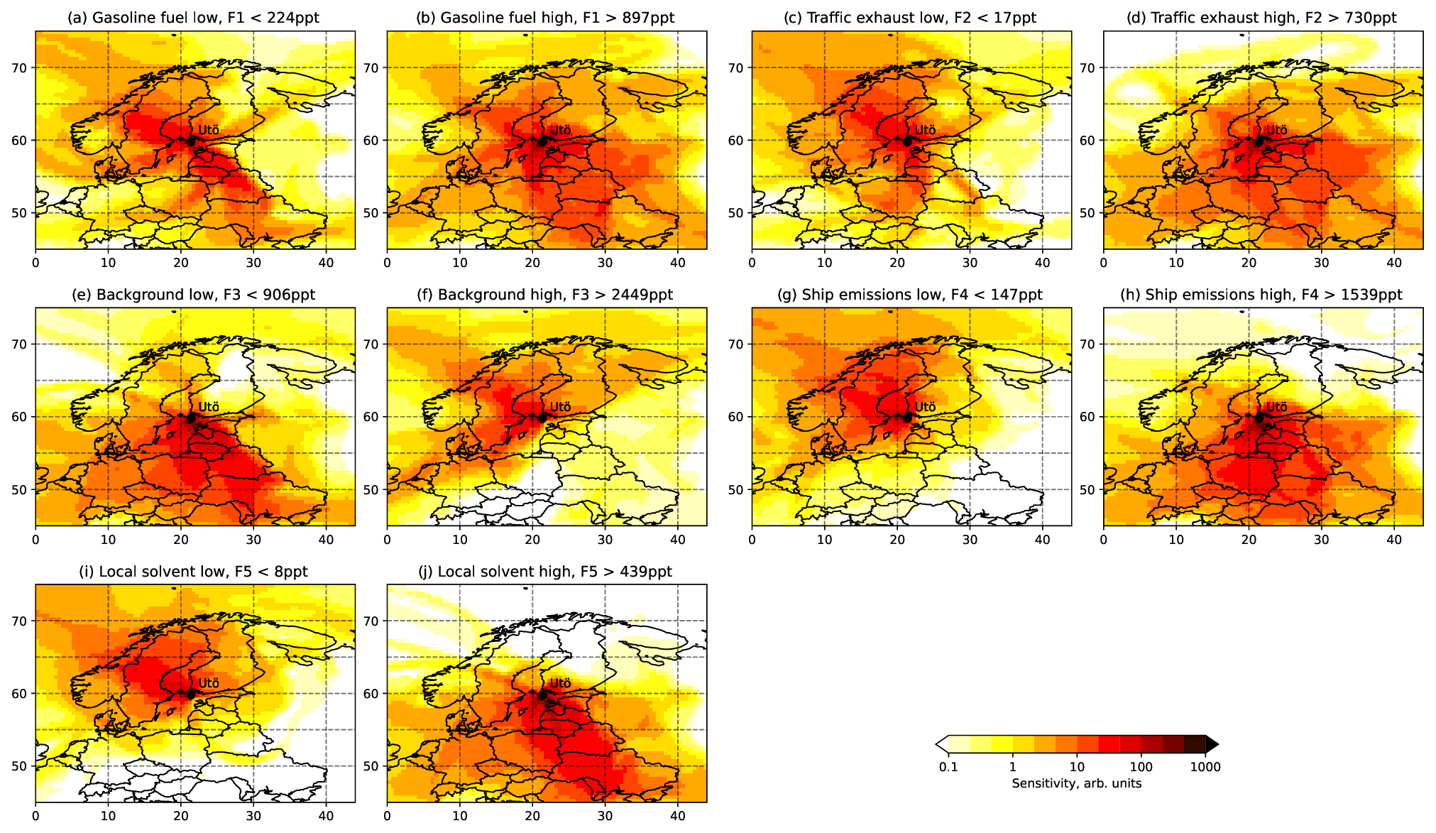
Figure 5 Sensitivity maps for low and high factor loadings showing the source area probabilities of factors (F1–F5).

Factor 2 (F2) was the traffic exhaust emission factor. It was characterized by the strong contribution of aromatic hydrocarbons (Fig. 3), which are known to be major compounds of traffic exhaust emissions (e.g. Hellén et al., 2006; Wang et al., 2020; Wu et al., 2020a). This factor made a high contribution, especially in the beginning of February during high wind speeds (Fig. 6). Wind direction distribution indicated that the main source was to the east of Utö in the direction of Saint Petersburg (Fig. 4). Sensitivity maps of F2 showed very similar source areas as for F1 (petrol) with contributions from Russia and the southern shore of the Gulf of Finland, the difference being that it also contained a substantial contribution from the Baltic states (Fig. 5).

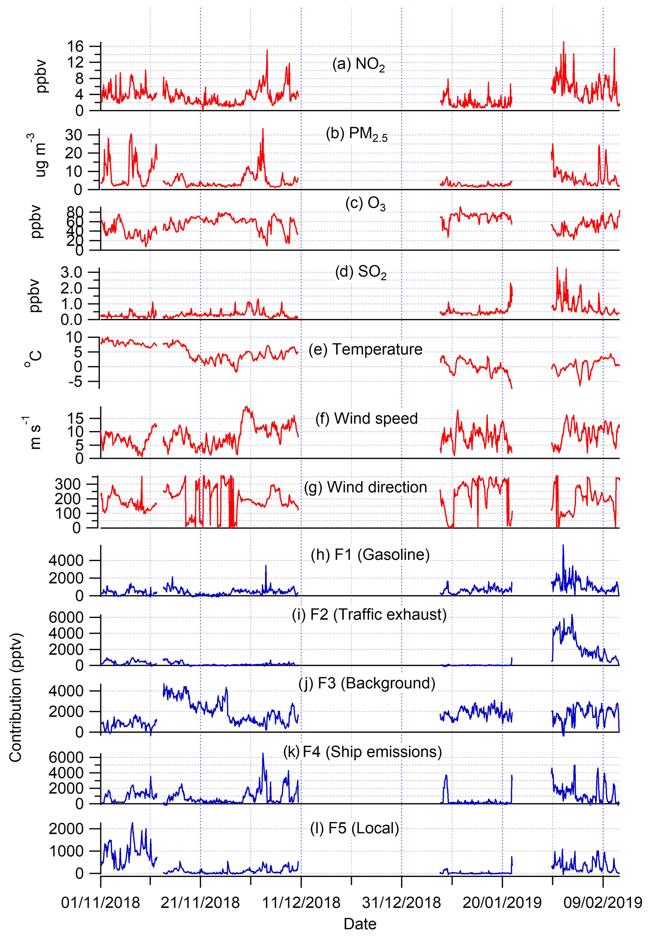
Figure 6 Time series of air pollutants (a–d; in red), meteorological parameters (e–g; in red), and PMF factor contributions (h–l; in blue) at Utö during the NMHC measurement periods in winter 2018–2019.

Factor 3 (F3) was identified as long-range-transported background air with a high contribution of the longest-living NMHCs, ethane, and propane (Fig. 3). The contribution of the factor over time was relatively stable compared to other factors (Fig. 6), and the highest contribution of the measured NMHCs, 42 %, came within this factor. Wind direction distribution was more scattered, as expected, for the regional background (Fig. 4), but the main source area was to the west and north-west from the site. The nearby shipping routes going to the Gulf of Bothnia and between the cities of Turku (Finland) and Stockholm (Sweden) are in that direction, and ships running on those routes use liquified natural gas (LNG), which is known to have ethane and propane emissions (Anderson et al., 2015) and could be influencing this factor as well. Also, sensitivity maps indicated that F3 got most of its contribution from Finland and Sweden and much lower contribution from the Baltic states and Russia (Fig. 5).

Factor 4 (F4) was identified as the shipping emission factor. It was characterized by the high contribution of ethene, propene, and ethyne, which are major NMHCs in ship emissions (Bourtsoukidis et al., 2019; Wu et al., 2020b). The variation in the factor contribution followed the variation in NO₂ and PM_2.5 (Fig. 6). Based on the wind direction distribution, the main source area coincided with the main ship route going to the Finnish and Russian harbours in the Gulf of Finland (Fig. 1b). Sensitivity maps of air masses (Fig. 5) also indicated a main contribution from southern and south-eastern sectors with quite uniform directional spawn. This ship emission factor made a 21 % contribution to the total measured NMHCs.

Factor 5 was interpreted as the local solvent factor. It was a significant source only of ethylbenzene and o-xylene (Fig. 3b). These compounds are well-known solvents, e.g. in paints and coatings (e.g. Castano et al., 2019; Song and Chun, 2021). However, F5 contribution to the total measured NMHCs was low at only 6 %. The wind direction probabilities indicated the local origin of the source to be in the direction of the village and harbour of Utö Island during low wind (Fig. 4). In November, when the wind direction changes to the north, contribution of this local factor decreases (Fig. 6). Based on the sensitivity maps (Fig. 5), F5 had a similar pattern as F4, with a much narrower high-contribution sector in the south-eastern direction from the measurement site.

The findings of the sensitivity maps were consistent with the wind analysis, being more specific for distant sources (F1–F3), for which the large-scale trajectories are important, and much less specific for local sources, whose contribution is primarily controlled by local winds.

3.2.2 Sources of NMHCs

Based on the PMF analyses, the main source of studied NMHCs at Utö Island was long-range-transported air masses (F3), with a 42 % contribution (Table 1). The strongest local/regional source was ship emissions (F4; 21 % contribution to the total NMHCs), followed by petrol fuel (F1) and traffic exhaust emissions (F2), with 15 % and 14 % contributions, respectively. In addition, there was a local solvent evaporation source (F5) with a 6 % contribution.

Table 1 Identification of the PMF factors and the mean contribution to the NMHC mixing ratios measured at the site.

Source contributions of individual NMHCs were highly variable (Fig. 3b). For the lightest alkanes, ethane and propane, long-range-transported background air was clearly the main source with 64 % and 50 % contributions, respectively. This is expected since compounds with long atmospheric lifetimes are known to accumulate in the atmosphere in northern latitudes during wintertime. Their relatively high wintertime mixing ratios are detected even in remote areas (Hellén et al., 2015; Solberg et al., 2020). Petrol fuel emissions (∼ 35 %) and background air (∼ 30 %) were major sources of butanes. For pentanes, the main source was petrol emissions, with a ∼ 50 % contribution. For the alkane with shortest atmospheric lifetime, 2-methylpentane, traffic exhaust emissions were the main source with a 62 % contribution.

Alkenes (ethene and propene) mainly originated from ship emissions with 81 % and 53 % contributions. For propene, long-range-transported background air was also a significant source with a 47 % contribution. Due to the relatively short atmospheric lifetime of propene, this is not expected. Uncertainties in defining a proper blank value for propene may have induced this. For other compounds, a blank was not detected or was not as significant. Ethyne was the only alkyne detected, and ship emissions were the major source for it with a 47 % contribution.

For aromatic hydrocarbons, traffic exhaust emissions were the major source with 45 %–65 % contributions. Based on the wind direction distribution, these emissions mainly originated from the east, the direction of the city of Saint Petersburg, 500 km to the east from site. For benzene, toluene, and o-xylene, ship emissions also resulted in 32 %, 21 %, and 13 % contributions, respectively. In addition, local solvent emissions contributed to the mixing ratios of ethylbenzene and o-xylene, with 46 % and 21 % contributions, respectively. Due to their shorter lifetime, these compounds have very low mixing ratios in remote areas, and therefore, as expected, long-range-transported background air did not result in a strong contribution.

For alkanes and aromatic hydrocarbons, the loading of the background factor (F3) had a clear correlation (R²= 0.93) with the logarithm of the compound's lifetime (Fig. 7). As expected, for compounds with the longest lifetime, the contribution was highest. However, based on benzene lifetime, a stronger impact of the background air would have been expected. A higher contribution of background air masses to benzene mixing ratios has been found even in the city of Helsinki in Finland (Hellén et al., 2006). This could indicate a stronger local source. However, the mixing ratios of benzene were not high, and it had a low signal-to-noise ratio, and, therefore, high uncertainties in the PMF solution and measurements of benzene were expected.

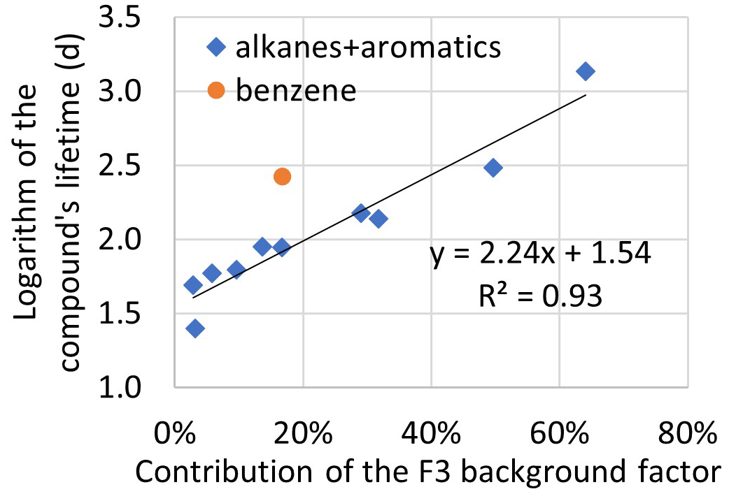
Figure 7 Correlation of the logarithm of a compound's lifetime (Hellén et al., 2015) with the contribution of the F3 background factor to the mixing ratio of the compound.

3.3 Mixing ratios of methanethiol

In addition to the NMHCs, we also detected methanethiol. Contrary to the usual annual cycle of anthropogenic VOCs, methanethiol had a maximum during spring and summer (Fig. 2). Therefore, it is expected to have a biogenic origin. At Utö, methanethiol mixing ratios started to increase at the end of April when the daily-mean ambient air and seawater temperatures were above 5 and 4 °C, respectively (Fig. 8). The mixing ratios increased simultaneously with seawater temperature in spring, and the maximum mixing ratios were measured at the end of May. The mixing ratios declined below detection limits in September. Total phytoplankton biomass in seawater was measured concurrently with the atmospheric VOCs during the period July–August, and it is plotted together with methanethiol in Fig. 8. Unfortunately, we do not have phytoplankton data from early summer due to underwater pump failure. There are many factors that affect the movement of substances from water to air and dilutions of emissions in the air, but the methanethiol mixing ratios seem to follow the total phytoplankton biomass in seawater, and the decrease in phytoplankton biomass may explain the decrease in the mixing ratios after mid-July.

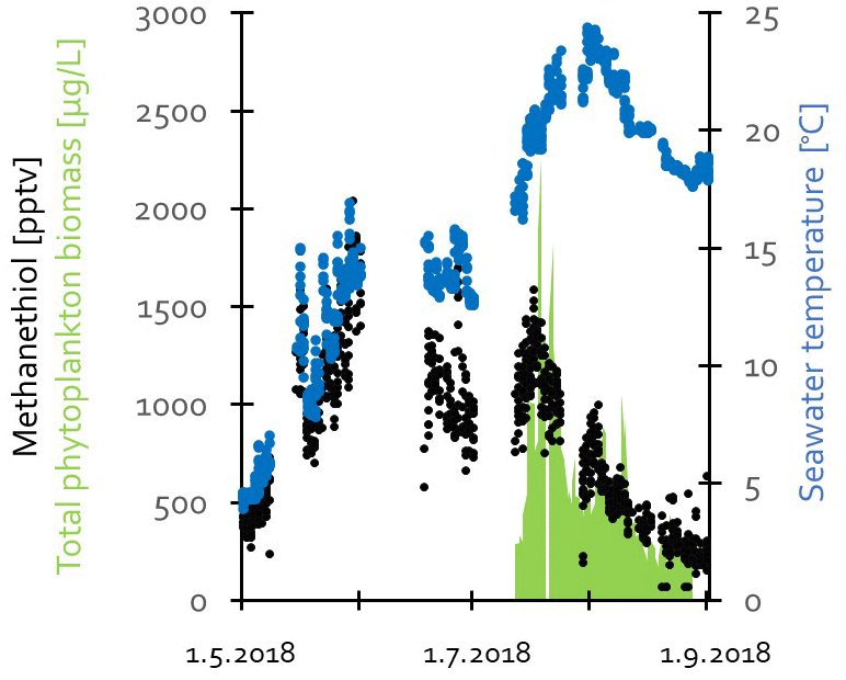
Figure 8 Methanethiol (CH₃SH) mixing ratios together with seawater temperature in May–August and total phytoplankton biomass in July–August 2018 at Utö.

Biogenic emissions of volatile organic compounds from vegetation are generally known to have exponential dependence on air/leaf/needle temperature (Guenther et al., 2012). Here, dependence of the mixing ratios of methanethiol on both ambient air and seawater temperatures was studied (Fig. 9). Even if phytoplankton were the source of the ambient air methanethiol, temperature may be a significant factor controlling its production by phytoplankton and its transfer from sea to atmosphere. The temperature dependence of the methanethiol mixing ratios varied over the season. In May, strong exponential dependence on both seawater (R²= 0.83) and ambient air (R²= 0.65) temperatures was found. In June, the mixing ratios did not correlate with seawater or ambient air temperatures (R²= 0.02 and 0.03, respectively). However, the measurements were within quite a narrow temperature range. In July, there was some dependence on ambient air (R²= 0.4) but no correlation with seawater temperature (R²= 0.07). In August, the correlation of the mixing ratios with seawater and ambient air temperatures was again high with R² being 0.83 and 0.62, respectively. The reason for these differences could be shifts in phytoplankton community composition and their physiological status, possible contributions from macroalgae vegetation from the shoreline, and meteorology.

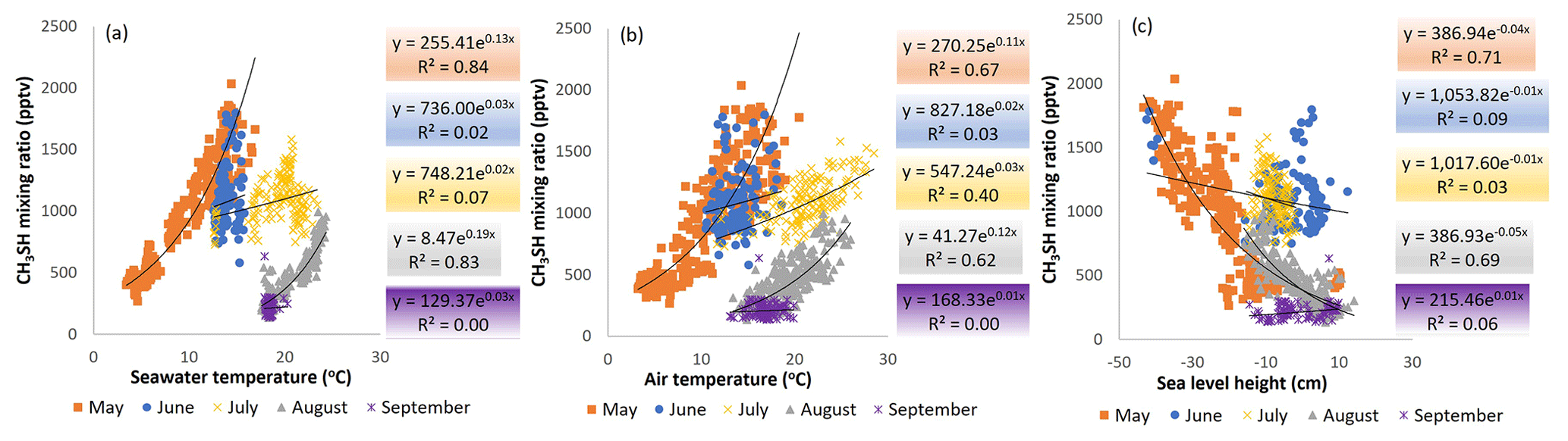
Figure 9 Dependence of methanethiol (CH₃SH) mixing ratios on (a) seawater temperature, (b) ambient air temperature, and (c) sea level height.

In addition to temperature, sea level height had a clear negative correlation with the methanethiol mixing ratios especially in May (R²= 0.69) and August (R²= 0.69; Fig. 9c). With lower sea levels, more macroalgae may be exposed to the ambient air and start decaying faster, inducing more methanethiol emissions. This strong negative correlation could indicate macroalgae being a significant source of methanethiol. In June and July, there was no correlation with sea level height, which indicates that other sources (e.g. phytoplankton) played a more important role. While seawater and ambient air temperature dependencies (Fig. 9a and b) were different for May and August, sea level height followed the same curve during both months (Fig. 9c).

The wind direction distribution (Fig. 10) indicates that the highest mixing ratios of methanethiol were measured during northernly winds (5–10 m s⁻¹). To the north of the site, there are wide archipelago areas with frequently occurring phytoplankton blooms and macroalgae as possible sources of methanethiol.

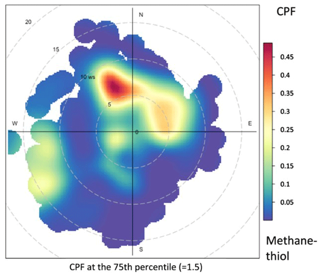
Figure 10 Probability function of distribution of wind direction and speed for the measured methanethiol mixing ratios. Dashed circles show the wind speed in 5 m s⁻¹ increments.

There is very little information available on methanethiol mixing ratios or emissions globally. Novak et al. (2022) measured a mean mixing ratio of 19 pptv at the Scripps Institution of Oceanography in La Jolla, CA, USA, during September 2019. The highest measured value was 217 pptv. Lawson et al. (2020) measured a mean mixing ratio of 18 pptv in the remote south-western Pacific Ocean in the summer of 2012. These values are clearly lower than those measured in this study in the Baltic Sea, where the highest monthly means were ∼ 1000 pptv. The coastal location with the adjacent macroalgae vegetation and high production of phytoplankton in the nutrient-rich and eutrophic Baltic Sea may explain these higher values. Leck and Rodhe (1991) found 15 times higher DMS concentrations compared to methanethiol in seawater in the Baltic Sea. Here, we did not detect DMS, but our method was not optimized for it, and it is possible that we do not capture it with our method.

Methanethiol is intensively malodorous. It has an odour threshold of 1000–2000 pptv. During warm weather with intensive phytoplankton blooms and decaying macroalgae on the shores of the island, the inhabitants of Utö are known to suffer due to a very bad smell. In our measurements, the odour threshold was exceeded often in the summer of 2018.

Novak et al. (2022) found that methanethiol emissions are dependent on wind speed, but in this study, we did not find any correlation of mixing ratios with wind speed. While wind might increase emissions, it also increases dilution in the air. In addition, there are several other factors that impact the mixing ratios, e.g. oxidation and mixing layer height, and therefore emissions and the factors impacting them are not expected to be directly comparable with mixing ratios.

It has been estimated that methanethiol could be a source of up to 30 % of the SO₂ formed in the marine boundary layer in coastal California, where clearly lower mixing ratios were measured than in this study (Novak et al., 2022). In our study, the methanethiol mixing ratios were high over several months and not just during short blooming periods (Fig. 2). This indicates that methanethiol could have a stronger contribution to SO₂ production in this area. More studies on methanethiol emissions are needed to confirm this.

4 Conclusions

The ambient air mixing ratios of NMHCs and methanethiol were studied at the marine research station on Utö Island in the Baltic Sea. The NMHC mixing ratios were typical of the northern rural/remote site. The seasonal variations in NMHCs followed a well-known cycle with maximum mixing ratios in winter and minimum during summer. The exception was methanethiol, which was identified here for the first time. It had a clear maximum in spring and summer.

For longer-living NMHCs in particular, the regional background was shown to be the major source. The contribution of the background had an exponential correlation with the lifetime of the measured alkanes and aromatic hydrocarbons. This gives confidence that PMF can produce valid information on the source apportionment of NMHCs also at rural/remote sites, where the ratios of these reactive compounds have been altered during transport from their sources to the site.

Of the local/regional sources, shipping had a strong impact especially on ethene, propene, ethyne, and benzene. For shorter-living NMHCs (aromatic hydrocarbons and 2-methylpentane), traffic emissions had a major effect. Wind distribution analyses indicated that these traffic emissions came from the direction of the main harbours/cities of the Gulf of Finland including the city of Saint Petersburg 500 km to the east of site. Petrol evaporative emissions which originated in the east had a strong impact on butane and pentane levels.

The mixing ratios of methanethiol followed the variations in seawater temperatures in spring and autumn. After mid-July, the mixing ratios started to decline, while seawater temperatures remained high. During that time, the abundance of phytoplankton in the seawater also declined, indicating phytoplankton as a possible source. The mixing ratios also negatively correlated with sea level height, especially in May and August. Macroalgae exposed to ambient air during low sea levels may start decaying faster and induce methanethiol emissions. These, together with ambient air temperature dependence, high summertime mixing ratios, and correlation with phytoplankton abundance gave indication of the biogenic origin of methanethiol possibly resulting from phytoplankton or macroalgae. The detected mixing ratios were higher than those found earlier in other areas and may be the source of the malodour detected on the island during strong phytoplankton blooms. This may also have a strong impact on local SO₂ production and new particle formation. More studies on methanethiol emissions and atmospheric impacts are needed to confirm these findings.