Correction of stratospheric age of air (AoA) derived from sulfur hexafluoride (SF₆) for the effect of chemical sinks

Observational monitoring of the stratospheric transport circulation, the Brewer–Dobson circulation (BDC), is crucial to estimate any decadal to long-term changes therein, a prerequisite to interpret trends in stratospheric composition and to constrain the consequential impacts on climate. The transport time along the BDC (i.e. the mean stratospheric age of air, AoA) can best be deduced from trace gas measurements of tracers which increase linearly with time and are chemically passive. The gas sulfur hexafluoride (SF₆) is often used to deduce AoA because it has been increasing monotonically since the ∼1950s, and previously its chemical sinks in the mesosphere have been assumed to be negligible for AoA estimates. However, recent studies have shown that the chemical sinks of SF₆ are stronger than assumed and become increasingly relevant with rising SF₆ concentrations.

To adjust biases in AoA that result from the chemical SF₆ sinks, we here propose a simple correction scheme for SF₆-based AoA estimates accounting for the time-dependent effects of chemical sinks. The correction scheme is based on theoretical considerations with idealized assumptions, resulting in a relation between ideal AoA and apparent AoA which is a function of the tropospheric reference time series of SF₆ and of the AoA-dependent effective lifetime of SF₆. The correction method is thoroughly tested within a self-consistent data set from a climate model that includes explicit calculation of chemical SF₆ sinks. It is shown within the model that the correction successfully reduces biases in SF₆-based AoA to less than 5 % for mean ages below 5 years. Tests using only subsampled data for deriving the fit coefficients show that applying the correction scheme even with imperfect knowledge of the sink is far superior to not applying a sink correction.

Furthermore, we show that based on currently available measurements, we are not able to constrain the fit parameters of the correction scheme based on observational data alone. However, the model-based correction curve lies within the observational uncertainty, and we thus recommend using the model-derived fit coefficients until more high-quality measurements are able to further constrain the correction scheme. The application of the correction scheme to AoA from satellites and in situ data suggests that it is highly beneficial to reconcile different observational estimates of mean AoA.

1 Introduction

The distributions of trace gases in the stratosphere are strongly influenced by the slow Equator-to-pole overturning circulation in the stratosphere, the Brewer–Dobson circulation (BDC). Most prominently, total column abundances of stratospheric ozone are maximized in mid- to high latitudes despite the strongest chemical production being in the tropics. The drive of this overturning circulation by wave dissipation, acting to drive the slow adiabatic rising and sinking as well as inducing wave stirring that subsequently leads to mixing, has been understood for many decades (Haynes et al., 1991; Butchart, 2014). However, dynamical measures of the overturning circulation like the residual circulation velocities are not observable. The distributions of trace gases rather serve to deduce measures of the circulation strength – fittingly given the initial definition of the BDC as tracer transport circulation (Brewer, 1949; Dobson, 1956).

A well-established measure to quantify BDC strength is the mean transport time from a reference surface (e.g. the tropical tropopause or the Earth's surface) to a point in the stratosphere, referred to as the mean stratospheric age of air (AoA) (Waugh and Hall, 2002). One advantage of this AoA measure is that it can be directly deduced from trace gas abundances; given an inert tracer whose surface abundance increases linearly with time, AoA is simply the lag time between the mixing ratio at the surface and the mixing ratio at a given point in the stratosphere. Strictly, this measures the transport time both within the troposphere and in the stratosphere, but as transport times from the surface to the tropical tropopause can be neglected compared to stratospheric transport times, AoA relative to the surface is still a good measure of the stratospheric transport circulation. However, such an ideal AoA tracer does not exist in reality. One gas that has often been used to derive AoA from observations is sulfur hexafluoride (SF₆). SF₆ is a well-suited AoA tracer since its surface abundances have increased monotonically since the ∼1950s, and its chemical sinks are located in the mesosphere and above, which have previously been assumed to have little influence on SF₆ abundances outside the winter polar vortices. A number of high-quality measurements of SF₆ from different platforms (in situ and satellite) have existed for many decades up until today (e.g. Andrews et al., 2001; Engel et al., 2009; Stiller et al., 2012; Haenel et al., 2015). While SF₆ surface abundances do not increase linearly, it has been shown that the non-linear increase in SF₆ can be corrected for in the derivation of AoA (Stiller et al., 2012; Fritsch et al., 2019). SF₆ has the advantage compared to the other common age tracer CO₂ that it has almost no seasonal cycle in emissions. The strong seasonal cycle in CO₂ complicates the AoA calculation in particular in the lower stratosphere (e.g. Andrews et al., 2001). Thus, SF₆ is, in principle, a useful and often-measured AoA tracer. However, it has become increasingly clear in recent years that the chemical sinks of SF₆ introduce substantial biases in AoA (e.g. Stiller et al., 2012; Ray et al., 2017; Kovács et al., 2017; Leedham Elvidge et al., 2018; Loeffel et al., 2022). It is strongly desirable to be able to correct for the effects of chemical sinks in SF₆ in order to use the existing and possible future observations of SF₆ to monitor the stratospheric transport circulation.

Loeffel et al. (2022) investigated the effects of chemical sinks on AoA derived from SF₆ in a global model and showed that the bias of AoA induced by the chemical sink grows with increasing mixing ratios. Thus, biases have been particularly strong since the 2000s. Furthermore, this effect can induce apparent positive trends in AoA, hampering efforts to deduce long-term circulation trends from SF₆-based AoA. In Loeffel et al. (2022) it was discussed that there is a compact relationship between ideal AoA and SF₆-based apparent AoA for AoA below a certain threshold. On this basis, it was suggested that it might be possible to correct observed SF₆-based AoA for the effects of chemical sinks. Here we follow up on this idea and develop a correction scheme for SF₆-based AoA. Firstly, theoretical considerations with simplifications are used to deduce a possible formulation of the correction scheme (Sect. 2). The strategy of the paper is to develop and test the correction scheme thoroughly within the self-consistent model world (Sect. 4, with the model being described in Sect. 3.1). This includes subsampling the model data to test the robustness of the correction against incomplete knowledge of the ideal AoA to apparent AoA relationship (Sect. 4.3). The next step is a comparison of the relation of SF₆-based AoA to AoA deduced from other tracers from observational data to the model relation. Ideally, the fit parameters for the correction scheme would be based on observational data alone; however, we show that current observations are not able to constrain the fit parameters (Sect. 5). Instead, we use fit parameters from the model and apply them to independent observations to test the performance of the correction scheme (Sect. 5). In Sect. 6 we summarize our findings, discuss the shortcomings and give recommendations on the application of the correction scheme.

2 Theoretical considerations for sink correction methods

In this section, we will lay out the theoretical basis for how chemical depletion of a tracer affects the derivation of mean AoA from this tracer. We will make various simplifying assumptions to derive analytical expressions for the effects of chemical sinks on tracer abundances and on the AoA derived from them. The climate model data introduced in Sect. 3.1 will serve to test how well-justified those assumptions are.

Generally, for any location, we can express the stratospheric tracer mixing ratio χ_s at time t for a tracer that is transported from a reference surface as

$$\begin{array}{}\text{(1)}& {\mathit{\chi }}_{\mathrm{s}}\left(t\right)=\underset{t^{\prime }=\mathrm{0}}{\overset{\mathrm{\infty }}{\int }}{\mathit{\chi }}_{\mathrm{0}}(t-t^{\prime })\exp (-t^{\prime }/\mathit{\tau }(t^{\prime }\left)\right)G(t^{\prime },t,x)\mathrm{d}{t}^{\prime },\end{array}$$

where t^′ denotes the transit time, χ₀(t) is the time series of the tracer mixing ratio at a reference surface, and G(t^′) represents Green's function and is equivalent to the distribution of transit times (often called the age spectrum). Note that Green's function is generally dependent on location x and on time t (hereafter those indices will be dropped for brevity without loss of generality). The exponential function in the integral represents the effects of chemical sinks on the tracer with transit-time-dependent and path-integrated lifetime τ. For simplicity, we will first consider a tracer with a linear increase at the reference surface before moving on to a tracer with a monotonic but non-linear increase.

2.1 Linearly increasing tracer

We assume a linearly increasing tracer with ${\mathit{\chi }}_{\mathrm{0}}={\mathit{\delta }}_{{\mathit{\chi }}_{\mathrm{0}}}t$. Given the definition of mean AoA as the first moment of the age spectrum ($\mathrm{\Gamma }={\int }_{t^{\prime }=\mathrm{0}}^{\mathrm{\infty }}{t}^{\prime }G\left(t^{\prime }\right)\mathrm{d}{t}^{\prime }$), AoA from a linearly increasing tracer can be calculated as the lag time between the tracer mixing ratio at the location of interest and the time series at the reference surface ($\mathrm{\Gamma }=t-{\mathit{\chi }}_{\mathrm{s}}\left(t\right)/{\mathit{\delta }}_{{\mathit{\chi }}_{\mathrm{0}}}$). We will refer to such estimated AoA without taking the effects of chemical sinks into account as the apparent AoA $\stackrel{\mathrm{̃}}{\mathrm{\Gamma }}$. In this case, the apparent AoA is given by

$$\begin{array}{}\text{(2)}& \begin{array}{rl}\stackrel{\mathrm{̃}}{\mathrm{\Gamma }}& =t-{\displaystyle \frac{{\mathit{\chi }}_{\mathrm{s}}\left(t\right)}{{\mathit{\delta }}_{{\mathit{\chi }}_{\mathrm{0}}}}}=t\left[\mathrm{1}-\underset{t^{\prime }=\mathrm{0}}{\overset{\mathrm{\infty }}{\int }}G\left(t^{\prime }\right)\exp \left({\displaystyle \frac{-t^{\prime }}{\mathit{\tau }}}\right)\mathrm{d}{t}^{\prime }\right]\\ & +\underset{t^{\prime }=\mathrm{0}}{\overset{\mathrm{\infty }}{\int }}{t}^{\prime }G\left(t^{\prime }\right)\exp \left({\displaystyle \frac{-t^{\prime }}{\mathit{\tau }}}\right)\mathrm{d}{t}^{\prime }.\end{array}\end{array}$$

We will now make two assumptions. Firstly, we assume that the mean AoA Γ is small compared to lifetime τ, which is generally the case for SF₆ within the stratosphere (in which case lifetime is on the order of 100 to 1000 years, and the mean AoA is less than 10 years). Thus, we can approximate $\exp \left(-\frac{t^{\prime }}{\mathit{\tau }}\right)\approx \mathrm{1}-\frac{t^{\prime }}{\mathit{\tau }}$. Secondly, we will make the assumption that the transit-time-dependent lifetime τ(t^′) can be replaced by the path-average lifetime τ_eff. This lifetime τ_eff is the path-average lifetime across all possible paths to the point of interest of the path-integrated lifetime τ(t^′), and we refer to this as the “effective” lifetime. Note that similar formulations have been used previously by Holzer and Waugh (2015), where they refer to this quantity as the “path-dependent inverse loss frequency”, and by Schoeberl et al. (2000) in their “average path assumption”.

With the two assumptions stated above, we can simplify Eq. (2) to

$$\begin{array}{}\text{(3)}& \stackrel{\mathrm{̃}}{\mathrm{\Gamma }}\approx t{\displaystyle \frac{\mathrm{\Gamma }}{{\mathit{\tau }}_{\mathrm{eff}}}}+\mathrm{\Gamma }-{\displaystyle \frac{\mathrm{1}}{{\mathit{\tau }}_{\mathrm{eff}}}}\underset{t^{\prime }=\mathrm{0}}{\overset{\mathrm{\infty }}{\int }}{t^{\prime }}^{\mathrm{2}}G\left(t^{\prime }\right)\mathrm{d}{t}^{\prime }.\end{array}$$

Using the expression for the width of the age spectrum ${\mathrm{\Delta }}^{\mathrm{2}}=\frac{\mathrm{1}}{\mathrm{2}}{\int }_{t^{\prime }=\mathrm{0}}^{\mathrm{\infty }}(t^{\prime }-\mathrm{\Gamma }{)}^{\mathrm{2}}G(t^{\prime })\mathrm{d}{t}^{\prime }$, one can rewrite the latter term as $\frac{\mathrm{1}}{{\mathit{\tau }}_{\mathrm{eff}}}\left(\mathrm{2}{\mathrm{\Delta }}^{\mathrm{2}}+{\mathrm{\Gamma }}^{\mathrm{2}}\right)$ and after some rearrangement obtain

$$\begin{array}{}\text{(4)}& \stackrel{\mathrm{̃}}{\mathrm{\Gamma }}\approx \mathrm{\Gamma }\left(\mathrm{1}+{\displaystyle \frac{\mathrm{1}}{{\mathit{\tau }}_{\mathrm{eff}}}}\left(t-\mathrm{2}{\displaystyle \frac{{\mathrm{\Delta }}^{\mathrm{2}}}{\mathrm{\Gamma }}}-\mathrm{\Gamma }\right)\right)\approx \mathrm{\Gamma }\left(\mathrm{1}+{\displaystyle \frac{t}{{\mathit{\tau }}_{\mathrm{eff}}}}\right).\end{array}$$

The latter approximation is justified given that the time t since start of emission of the tracer (for SF₆ about 1950s) is around 1 order of magnitude larger (on the order of 10 years) than the mean AoA Γ and the ratio of moments $\frac{{\mathrm{\Delta }}^{\mathrm{2}}}{\mathrm{\Gamma }}$ (which are both on the order of 1; see e.g. Fritsch et al., 2019). This approximation holds less well in earlier years (1960s to 1970s), but given that the correction at those times is small, this poses no major issue. Thus, this approximated expression states that the apparent AoA differs from the true AoA Γ by a factor of $(\mathrm{1}+\frac{t}{{\mathit{\tau }}_{\mathrm{eff}}})$, which increases as time progresses (due to the increasing tracer mixing ratios; see discussion in Loeffel et al., 2022). The other necessary parameter for estimating the effects of chemical sinks on AoA is the effective lifetime. Since chemical sinks of SF₆ are located in the upper stratosphere and the mesosphere, the effective lifetime is location-dependent. For the correction scheme proposed here, we will parameterize the effective lifetime as a function of AoA. The relation of the effective lifetime to AoA is expected to bear latitudinal dependence, as is discussed in Sect. 4.1. The effective lifetime can be calculated from simultaneous data of SF₆-derived apparent AoA and AoA based on another tracer that is unaffected by the chemical sinks via the relation derived above:

$$\begin{array}{}\text{(5)}& {\mathit{\tau }}_{\mathrm{eff}}\left(\mathrm{\Gamma }\right)=t{\left({\displaystyle \frac{\stackrel{\mathrm{̃}}{\mathrm{\Gamma }}}{\mathrm{\Gamma }}}-\mathrm{1}\right)}^{-\mathrm{1}}.\end{array}$$

We deduce this relationship based on model data and then parameterize the effective lifetime as a function of ideal AoA (Γ) via different fit functions (exponential and polynomial), and the estimated parameters then serve as input for the correction scheme.

2.2 Non-linearly increasing tracer

In the next step, we extend the formulations given above to correct for a non-linearly increasing tracer, as is the case for SF₆. To account for the non-linear increase in the reference time series, we linearize the tropospheric time series ${\mathit{\chi }}_{\mathrm{0}}(t-t^{\prime })$ around the average transit time $t^{\prime }={\mathrm{\Gamma }}_{\mathrm{0}}$ so that

$$\begin{array}{}\text{(6)}& {\mathit{\chi }}_{\mathrm{0}}(t-t^{\prime })\approx {\mathit{\chi }}_{\mathrm{0}}(t-{\mathrm{\Gamma }}_{\mathrm{0}})+{\displaystyle \frac{\partial {\mathit{\chi }}_{\mathrm{0}}(t-{\mathrm{\Gamma }}_{\mathrm{0}})}{\partial t}}\cdot ({\mathrm{\Gamma }}_{\mathrm{0}}-t^{\prime }).\end{array}$$

Inserting this expression into Eq. (1) for a passive tracer named ${\mathit{\chi }}_{\mathrm{s}}^{\mathrm{p}}$ (i.e. $\exp (-t^{\prime }/\mathit{\tau }(t^{\prime }\left)\right)=\mathrm{1}$) and solving for Γ yields

$$\begin{array}{}\text{(7)}& \mathrm{\Gamma }={\displaystyle \frac{{\mathit{\chi }}_{\mathrm{0}}(t-{\mathrm{\Gamma }}_{\mathrm{0}})-{\mathit{\chi }}_{\mathrm{s}}^{\mathrm{p}}\left(t\right)}{\frac{\partial {\mathit{\chi }}_{\mathrm{0}}(t-{\mathrm{\Gamma }}_{\mathrm{0}})}{\partial t}}}+{\mathrm{\Gamma }}_{\mathrm{0}}.\end{array}$$

Note that this is not the common way to account for non-linearity when deriving AoA from a non-linearly increasing tracer. Usually, either a convolution with the age spectrum or a second-order polynomial fit to the reference time series is used (Engel et al., 2009; Stiller et al., 2012; Fritsch et al., 2019). The simple linearization of the tropospheric reference time series only approximates the local slope. For the mean age calculation, the time-evolving slope over all transit times that contribute to the age spectrum is important. However, for the sink correction we find that the approximation of linearization around a certain mean age proves to work well (as shown in the following in Sect. 4.2).

To obtain the relationship between apparent age and the true ideal age, we insert the chemically depleted tracer mixing ratio χ_s(t) instead of the passive tracer in Eq. (7), which after some rearrangement gives

$$\begin{array}{}\text{(8)}& \begin{array}{rl}\stackrel{\mathrm{̃}}{\mathrm{\Gamma }}& =\left(-{\displaystyle \frac{{\mathit{\chi }}_{\mathrm{0}}(t-{\mathrm{\Gamma }}_{\mathrm{0}})}{\frac{\partial {\mathit{\chi }}_{\mathrm{0}}(t-{\mathrm{\Gamma }}_{\mathrm{0}})}{\partial t}}}-{\mathrm{\Gamma }}_{\mathrm{0}}\right)\underset{t^{\prime }=\mathrm{0}}{\overset{\mathrm{\infty }}{\int }}G\left(t^{\prime }\right)\exp \left({\displaystyle \frac{-t^{\prime }}{\mathit{\tau }}}\right)\mathrm{d}{t}^{\prime }\\ & -\underset{t^{\prime }=\mathrm{0}}{\overset{\mathrm{\infty }}{\int }}{t}^{\prime }G\left(t^{\prime }\right)\exp \left({\displaystyle \frac{-t^{\prime }}{\mathit{\tau }}}\right)\mathrm{d}{t}^{\prime }+{\displaystyle \frac{{\mathit{\chi }}_{\mathrm{0}}(t-{\mathrm{\Gamma }}_{\mathrm{0}})}{\frac{\partial {\mathit{\chi }}_{\mathrm{0}}(t-{\mathrm{\Gamma }}_{\mathrm{0}})}{\partial t}}}+{\mathrm{\Gamma }}_{\mathrm{0}}.\end{array}\end{array}$$

We define a time-dependent function F_t(t) as the ratio of the reference mixing ratio to its temporal gradient:

$$\begin{array}{}\text{(9)}& F_t\left(t\right)={\displaystyle \frac{{\mathit{\chi }}_{\mathrm{0}}(t-{\mathrm{\Gamma }}_{\mathrm{0}})}{\frac{\partial {\mathit{\chi }}_{\mathrm{0}}(t-{\mathrm{\Gamma }}_{\mathrm{0}})}{\partial t}}}.\end{array}$$

We make the same assumptions as for Eq. (4), yielding the following approximate relation of apparent AoA to ideal AoA:

$$\begin{array}{}\text{(10)}& \begin{array}{rl}\stackrel{\mathrm{̃}}{\mathrm{\Gamma }}& \approx \mathrm{\Gamma }\left(\mathrm{1}+{\displaystyle \frac{\mathrm{1}}{{\mathit{\tau }}_{\mathrm{eff}}}}\left(F_t\left(t\right)+{\mathrm{\Gamma }}_{\mathrm{0}}-\mathrm{2}{\displaystyle \frac{{\mathrm{\Delta }}^{\mathrm{2}}}{\mathrm{\Gamma }}}-\mathrm{\Gamma }\right)\right)\\ & \approx \mathrm{\Gamma }\left(\mathrm{1}+{\displaystyle \frac{F_t\left(t\right)}{{\mathit{\tau }}_{\mathrm{eff}}}}\right).\end{array}\end{array}$$

The latter approximation is even slightly better-justified than for the linear tracer (see Eq. 4) because of the near cancellation of Γ and Γ₀. Thus, we obtain a similar expression as for the linearly increasing tracer (Eq. 4) but replace the linear time dependence t with the time-dependent function F_t(t). If the reference tracer mixing ratio increases linearly, Eq. (10) collapses to Eq. (4).

2.3 Correction scheme

The correction scheme we propose here is based on Eq. (10) and contains the following steps:

1. For any pair of given data of apparent and ideal AoA (${\stackrel{\mathrm{̃}}{\mathrm{\Gamma }}}_i$, Γ_i) observed at a certain time t_i, the effective lifetime is calculated based on ${\mathit{\tau }}_{\mathrm{eff}}=F_t\left(t_i\right)/({\stackrel{\mathrm{̃}}{\mathrm{\Gamma }}}_i/{\mathrm{\Gamma }}_i-\mathrm{1})$.

2. A function is fitted to parameterize τ_eff as a function of ideal AoA (Γ). In Sect. 4.1, we test an exponential fit function and polynomial fit functions of different orders. The fits are performed over a limited range of ideal AoA values (in this case 1 to 5 years; see Sect. 4.1).

3. Given the parameters from the fit and the time-dependent function based on the reference time series F_t(t), the relation between $\stackrel{\mathrm{̃}}{\mathrm{\Gamma }}$ and Γ is given for any time and can be used to correct SF₆-based apparent AoA. Since the relation between $\stackrel{\mathrm{̃}}{\mathrm{\Gamma }}$ and Γ cannot be analytically inverted (due to the non-linear dependence of τ_eff on Γ), we calculate $\stackrel{\mathrm{̃}}{\mathrm{\Gamma }}$ for a range of ideal mean ages in practice, and Γ is estimated from $\stackrel{\mathrm{̃}}{\mathrm{\Gamma }}$ via linear interpolation. AoA values beyond the range for which the fit was performed in the previous step (in this case for ideal AoA > 5 years) are treated in the following way – in the case of the exponential fit, the exponential fit function is evaluated also beyond AoA > 5 years. In the case of the polynomial fit, this would lead to problems as the polynomial is not well constrained outside the fit range and does not increase monotonically. Therefore, the polynomial is not evaluated for AoA > 5 years, but the values are extrapolated linearly.

2.4 Time-dependent function for non-linear increase

The time-dependent function F_t(t) takes the non-linear increase in the reference mixing ratio time series into account and is defined as the ratio of the mixing ratio and its temporal slope at a given time as given by Eq. (9).

The reference SF₆ time series at the surface is shown in Fig. 1a for both the best estimate based on surface observations (orange) and the time series taken from the global model data (blue). As can be seen, the two time series are close to identical. Nevertheless, in the remainder of the paper the model time series is used for model SF₆ data, and the observational time series is used for correcting observed SF₆-based AoA (in Sect. 5). Figure 1b shows the temporal gradient in the reference time series. Function F_t(t) (Fig. 1c) is calculated based on the annual mean time series of SF₆, where the gradient in the denominator of F_t(t) is calculated as the centred difference over 5 years. We find that in practice the offset mean AoA (Γ₀) of 4 years gives the best results, but generally results were found to be robust with respect to small variations in the choice of the offset mean AoA and also of the period for the gradient calculation. The values of F_t from the model versus observational time series only show differences in the earlier years (the 1950s and less so in the 1970s), which have negligible effects on the results presented in the remainder of the paper.

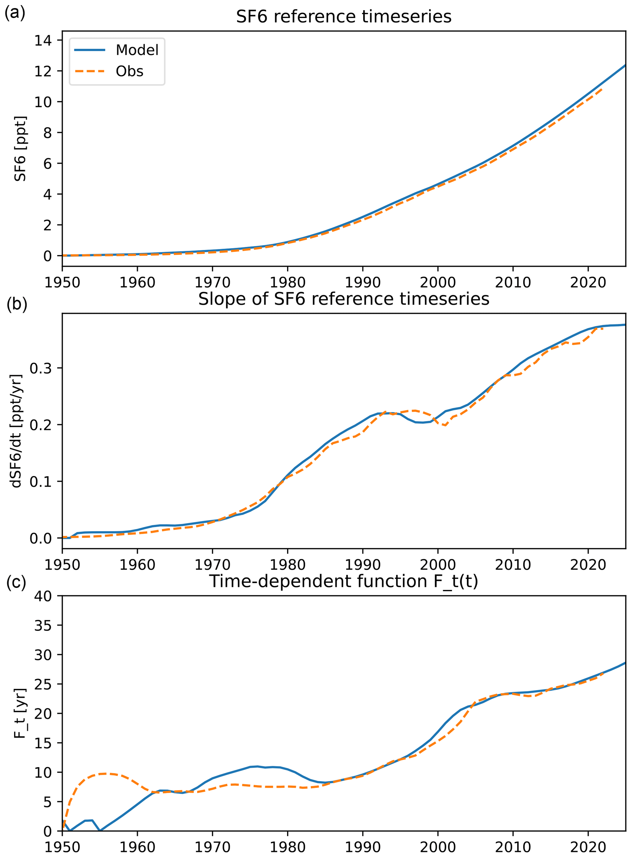
Figure 1 (a) Reference time series of SF₆ mixing ratios at the surface based on observations (dashed orange; updated version from Engel et al., 2009) and taken from the lowest level of the global model (blue; see  Jöckel et al., 2016, for the description of SF₆ lower-boundary data). (b) The temporal gradient of the two time series calculated as the centred difference over 5 years. (c) The time-dependent function F_t(t) defined as the ratio of the mean to the gradient and shifted by Γ₀= 4 years.

3 Data and model description

3.1 The ECHAM/MESSy Atmospheric Chemistry (EMAC) time slice simulation

We use the ECHAM/MESSy Atmospheric Chemistry (EMAC) model, which is a numerical chemistry and climate simulation system that includes submodels describing tropospheric and middle-atmospheric processes and their interaction with oceans, land and human influences (Jöckel et al., 2010). It contains the fifth-generation European Centre Hamburg general circulation model (ECHAM5, Roeckner et al., 2006) as the dynamical core atmospheric model and uses the second version of the Modular Earth Submodel System (MESSy2) to link multi-institutional computer codes. The physics subroutines of the original ECHAM code have been modularized and re-implemented as MESSy submodels and have been continuously further developed.

For the present study we applied EMAC (MESSy version 2.54.0; Jöckel et al., 2010, 2016) in the T42L90MA-resolution, i.e. with a spectral truncation of T42, which corresponds to a quadratic Gaussian grid of ∼ 2.8° × ∼2.8 ° in latitude and longitude and with 90 hybrid pressure levels in the vertical that reach up to 0.01 hPa. The applied model setup comprises the basic submodels for dynamics, radiation, clouds and diagnostics (AEROPT, CLOUD, CLOUDOPT, CVTRANS, E5VDIFF, GWAVE, ORBIT, OROGW, PTRAC, QBO, RAD, SURFACE, TNUDGE, TROPOP and VAXTRA; see Jöckel et al., 2005, 2010, for details) and the submodel SF₆. The submodel SF₆ is used to explicitly calculate the chemical sinks of SF₆ in the middle atmosphere. The calculations are based on the reaction scheme by Reddmann et al. (2001); details of the submodel are provided in Loeffel et al. (2022), but here we summarize the most important points. For electron-attachment-based SF₆ degradation, the electron field by Brasseur and Solomon (1986) is used and UV photolysis of SF₆ is not included as its loss rate is several orders of magnitude weaker than that of electron attachment up to about 100 km. Further reactions considered are photodetachment of SF${}_{\mathrm{6}}^{-}$ (Datskos et al., 1995); destruction of SF${}_{\mathrm{6}}^{-}$ by atomic hydrogen, hydrogen chloride and ozone (Huey et al., 1995); and stabilization of SF${}_{\mathrm{6}}^{-}$ excited by collisions, as well as autodetachment of SF${}_{\mathrm{6}}^{-}$. The autodetachment rate was set to 10⁶ s⁻¹, and to compute the photodetachment rate of SF${}_{\mathrm{6}}^{-}$, we use the extraterrestrial solar photon flux with no attenuation of the UV-photon flux (see Reddmann et al., 2001), as provided by WMO (1986). The overall global lifetime of SF₆ in the stratosphere and mesosphere is around 1900 years in the model (Loeffel et al., 2022). In general, the atmospheric SF₆ lifetime is subject to large uncertainties, with recent estimates ranging from about 800 to 3000 years (Ray et al., 2017; Kovács et al., 2017; Kouznetsov et al., 2020), encompassing the SF₆ lifetime in the EMAC model.

The simulation setup is designed as a time slice simulation with climate conditions of the year 2000. This means that climatologies of the 1995–2004 period of the greenhouse gases (GHGs) CO₂, CH₄, N₂O and O₃; the sea surface temperatures (SSTs); and the sea ice concentrations (SICs) are prescribed as monthly means. The Earth System Chemistry Integrated Modelling (ESCiMo) RC1-base-07 simulation (see Jöckel et al., 2016) data set was taken for the GHGs, and the Hadley Centre Sea Ice and Sea Surface Temperature (HadISST) data set (which was also used for the RC1-base-07 simulation) was taken for SSTs and SICs. The CCMI-1 volcanic aerosol data (for their effect on infrared radiative heating; see Arfeuille et al., 2013; Morgenstern et al., 2017) are prescribed, and the quasi-biennial oscillation (QBO) is nudged (see Jöckel et al., 2016). Moreover, the 1995–2004 average of the reactant species for the SF₆ sinks, namely HCl, H, N₂, O₂, O(³P) and O₃ from the RC1-base-07 simulation, are prescribed. Other than the SF₆ submodel, no interactive chemistry is activated in the simulations for this study. Note that in contrast to the climate conditions, the SF₆ lower boundary conditions are prescribed transiently over the period of the simulation with values starting in year 1950. This simulation has also been used in Loeffel et al. (2022) and therein was referred to as the TS2000 simulation. The setup is designed to investigate the effects of the SF₆ sinks under constant climate conditions and was chosen for this study to better isolate the effects of the SF₆ sinks without the influence of model-dependent secular trends in circulation and composition. It was shown by Loeffel et al. (2022) that the transient evolution of circulation and composition only has minor influences on the difference in ideal AoA compared to apparent AoA so that a transient simulation would give similar results to the time slice simulation in terms of the sink correction scheme.

We use the same AoA tracers as described in Loeffel et al. (2022) and in particular the linearly increasing ideal AoA tracer and two SF₆-tracers, one without chemical depletion and one with chemical depletion. AoA is calculated from the tracer mixing ratios as described in Loeffel et al. (2022), following Fritsch et al. (2019). In brief, we correct for the non-linear increase in the reference time series in the calculation of AoA from the SF₆ tracers via a polynomial fit method (with the parameter of the moment ratio of 1.0 and the fraction of input of 95 %; see Fritsch et al., 2019, for details). With this method, the passive SF₆ tracer results in almost identical AoA to the ideal, linearly increasing AoA tracer. In the following sections, we use the two SF₆ tracers with and without sinks and refer to the AoA from SF₆ without sink as “ideal” AoA and to AoA from SF₆ with sink as “apparent” or SF₆-based AoA.

3.2 Observational data

3.2.1 Aircraft and balloon data

Concurrent measurements of SF₆ and other, alternative age tracers are necessary to constrain the relationship between ideal and apparent AoA based on observations. Here, we use a number of such measurements available from aircraft and balloon campaigns spanning a period of 21 years (1997 to 2017) taken during different seasons and at different latitudes (see Fig. 2 for an overview).

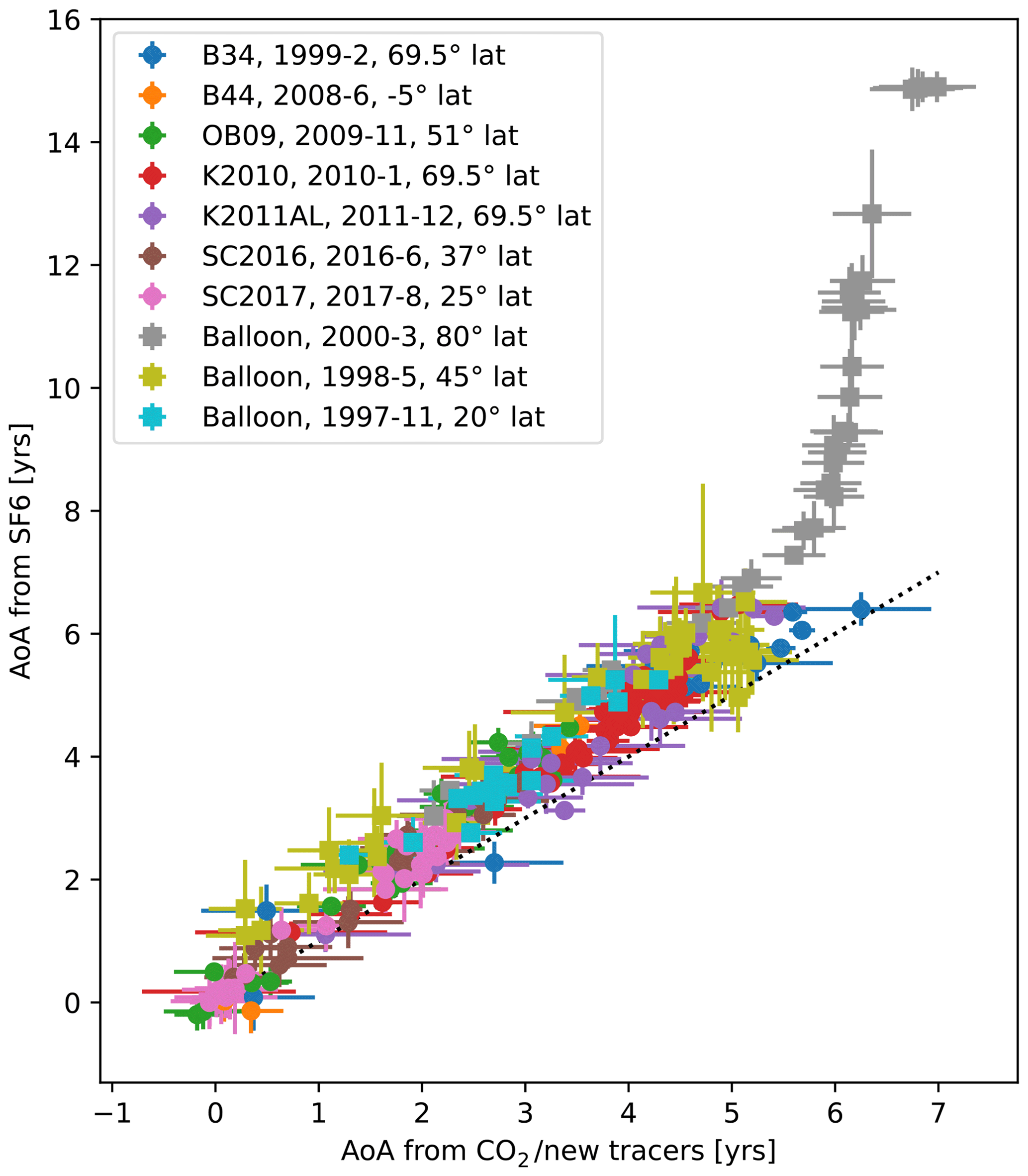
Figure 2 Available observational data pairs of AoA from SF₆ (y axis) and AoA from CO₂ (for the three balloon flights) or the average AoA from up to five alternative age tracers (x axis). Data are taken from different balloon and aircraft campaigns (see legend, which includes the information on the year and month and latitude of each observation; see text for details). Error bars represent 1 standard deviation, and the dotted line is the 1:1 line.

Leedham Elvidge et al. (2018) described the stratospheric observations of a set of inert trace gases and demonstrated their usefulness as AoA tracers, including a comparison to SF₆-based AoA. The five species are CF₄, C₂F₆, C₃F₈, CHF₃ (HFC-23) and C₂HF₅ (HFC-125), all of which result in slightly lower AoAs as compared to SF₆, with the discrepancy increasing with increasing AoA (see Fig. 2). This data set is based on air samples collected during several high-altitude balloon (labelled B34 and B44 in Fig. 2) and aircraft (labelled OB09, K2010, K2011AL and SC2016 in Fig. 2) campaigns in the tropics, mid-latitudes and high latitudes. It was subsequently augmented by AoA data from a further aircraft campaign (SC2017; Adcock et al., 2021).

The balloon data from 1997, 1998 and 2000 come from in situ measurements of SF₆ and CO₂ taken during the Observations of the Middle Stratosphere (OMS) and the SAGE III Ozone Loss and Validation Experiment (SOLVE) campaigns (Volk et al., 1997; Andrews et al., 2001; Moore et al., 2003; Ray et al., 2017). The mean ages were calculated differently for each trace gas, although they both use a variation on the lag technique. The sampling rates were also different between the instruments measuring each trace gas so the points shown in Fig. 2 for these flights were chosen based on a time coincidence of ±30 s.

3.2.2 Satellite data

The Michelson Interferometer for Passive Atmospheric Sounding (MIPAS) was an FTIR spectrometer on the Envisat satellite. It scanned the atmosphere from July 2002 to April 2012 in the altitude range between 6 and 70 km. During this period, about 2 million SF₆ profiles covering the entire globe and measured during the day and night were obtained. The retrieval of SF₆ profiles from the radiance spectra has been described previously (Stiller et al., 2008, 2012; Haenel et al., 2015). The data version used here has been retrieved following the approach described by Haenel et al. (2015), however, using newer absorption cross sections of SF₆ (Harrison, 2020) and accounting for a trichlorofluoromethane (CFC-11) band in the vicinity of the SF₆ signature (Harrison, 2018). This SF₆ data record is publicly available at https://doi.org/10.5445/IR/1000139453 (Stiller et al., 2021).

Moreover, we use AoA deduced from N₂O from the GOZCARDS (Global OZone Chemistry And Related trace gas Data records for the Stratosphere; Froidevaux et al., 2015) satellite product, as produced by Linz et al. (2017). The N₂O data are available for the years 2004–2012 and are based on observations by the Atmospheric Chemistry Experiment Fourier-transform spectrometer (ACE-FTS) for 2004–2010 and by the microwave limb sounder aboard the Aura satellite (Aura MLS) for 2004–2012. The AoA product relies on an empirical relation between CO₂-based AoA and N₂O as found by Andrews et al. (2001), accounting for the tropospheric trend in N₂O (Linz et al., 2017).

4 Testing the correction scheme in a global model

In this section, we use self-consistent model data to develop a sink correction scheme based on the concept laid out in Sect. 2. We start with an overview of the simulated relation between ideal and SF₆-based apparent AoA. Figure 3 shows the difference between ideal AoA and apparent AoA derived from the chemically depleted SF₆ tracer as a function of ideal AoA. As found by Loeffel et al. (2022), AoA differences due to chemical sinks increase approximately linearly for AoA lower than about 4 years and increase very strongly for older AoA values. The AoA difference increases from the 1960s to the 2020s due to the increasing mixing ratios of SF₆ (see Fig. 3a). The increase in differences is smaller in the first decades, when the SF₆ growth rates are small (see Fig. 1), and these differences increase more strongly with the stronger growth rates after ∼1990. The seasonal and latitudinal variations in the AoA differences are highlighted in Fig. 3b for one specific year (2015). The relation of ideal to apparent AoA is generally found to be quite compact for AoA below about 4 years. Variations with latitude and season are found in the ideal AoA values for which the difference starts to strongly increase; the strong increase in the AoA difference is found at lower ideal AoA values for tropical air compared to high latitudes. The contrast of tropical to high-latitude air is discussed in more detail in the next section. Generally, the mostly compact relationship between ideal and apparent AoA is promising for our aim to deduce a correction method that is valid globally.

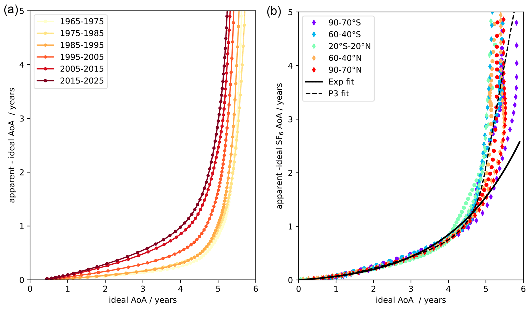
Figure 3 (a) Mean AoA from the ideal tracer plotted against the difference in apparent mean AoA derived from the non-linearly increasing SF₆-like tracer to ideal mean AoA from the TS2000 model simulations for global and decadal averages from year 5–15 (equivalent to 1965–1975 in SF₆ emissions, yellow) to year 55–65 (equivalent to 2015–2025, dark red). (b) Same as (a) but showing values for individual latitude bands and seasons for the year 2015, with circles denoting DJF and diamonds denoting JJA, colour-coded by latitude band (see legend). The black fit lines are the global mean fits used for the correction; see Sect. 4.1 for details.

Our strategy in developing the correction scheme is as follows. The first step is to parameterize the effective lifetime as a function of AoA using different fit functions (exponential or polynomial; see Sect. 4.1). We put particular focus on testing whether the fit coefficients change over time and how strongly they vary with latitude. Note that we have tested all shown diagnostics first with a pair of linearly increasing tracers (one with and one without chemical sink), but since we found very similar results for the non-linearly (SF₆-like) increasing tracer, we only show results for the latter, more realistic case. We then apply the correction schemes with fit coefficients from the model to the model data themselves (Sect. 4.2) to quantify to what degree the biases in SF₆-derived apparent AoA can be eliminated by the sink correction. This serves to decide which fit function performs best and how much the results improve through latitude-dependent fit coefficients compared to global uniform fit coefficients. Finally, in Sect. 4.3 it is tested how the limited availability of data in space and time impacts the fit coefficients and the subsequent correction, as will be relevant for the application to observational data.

4.1 Fit coefficients for different fitting methods

We first present two exemplary profiles of apparent AoA and ideal AoA, one in the tropics (10° S–10° N) and one over the south pole (80–90° S), arbitrarily chosen for the year 2000. In Fig. 4, the difference between apparent and ideal AoA is shown as a function of ideal AoA (Fig. 4a; similar to Fig. 3 but restricted to lower AoA values), showing the strong, non-linear increase in the AoA difference with increasing ideal AoA. For ideal AoA of up to about 4 years, the difference between apparent and ideal AoA is lower for tropical than for polar latitudes. This can be understood from observing a lower fraction of old air in the tropics compared to the high latitudes for a given AoA, i.e. less weight on the tail of the AoA spectrum (see e.g. Ploeger and Birner, 2016). The older air is more likely to be depleted in SF₆. For AoA above about 4 years, on the other hand, the difference between apparent and ideal AoA is larger in the tropics compared to at high latitudes. Ideal AoA of 4 years is located at a pressure level of around 7 hPa in the tropics but at a pressure level as low as around 60 hPa in high latitudes. Thus, the tropical air with ideal AoA above about 4 years is located much higher in the atmosphere and is therefore closer to the region where chemical sinks are active. This likely explains the strong increase in the apparent AoA already for lower ideal AoA compared to at high latitudes. Next to the annual mean profiles, shaded regions display the variation over the year. The seasonal cycle in the ideal–apparent AoA relation is very small in the tropics (see light-blue shading in Fig. 4a), whereas it is more pronounced at high latitudes for AoA values above about 4 years. Specifically, the AoA difference for a given ideal AoA value rises strongly in early spring (around November; not shown). This sudden increase in apparent AoA for ideal AoA of around 5 years is due to a sudden rise in the AoA isosurface – while the 5-year contour is located at around 30 to 40 hPa in winter, it rises in altitude to above 10 hPa in spring (not shown); thus, we are looking at a different air mass. If we analyse the difference between apparent and ideal AoA on a fixed pressure level (e.g. 20 hPa), this difference is highest in late winter just before the polar vortex breaks down (October) and the strong downwelling resulted in the accumulation of SF₆-depleted air over winter in the stratosphere. However, apart from in spring at high latitudes, the relationship between ideal and apparent AoA does not have a strong seasonal cycle (see also Fig. 3), and we will consider only annual mean profiles for performing the fits hereafter.

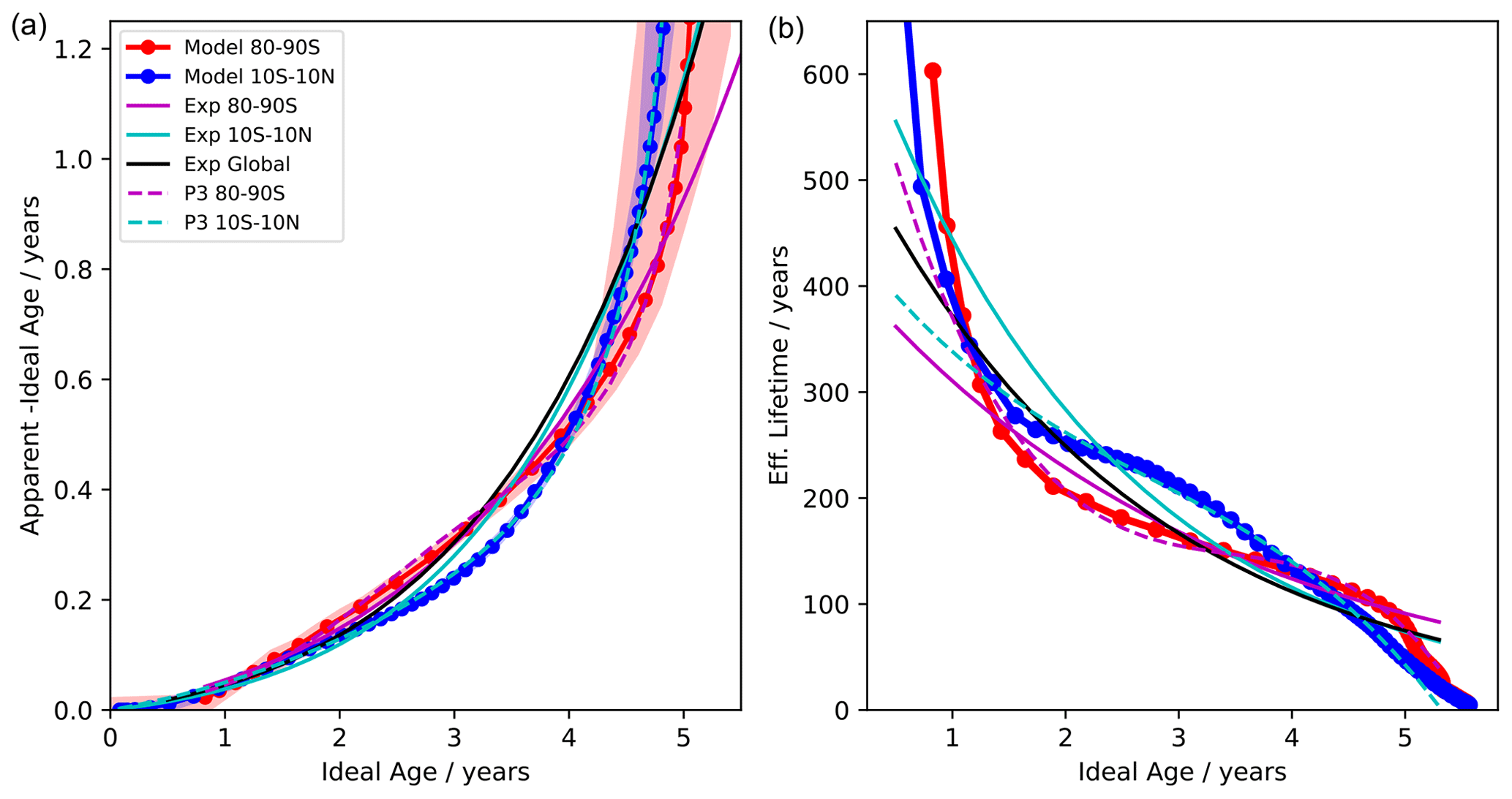
Figure 4 (a) Difference between apparent and ideal AoA for annual mean profiles of the year 2000 in the tropics (blue) and southern high latitudes (red) as a function of ideal mean age. The range of monthly mean values is shown as the shaded regions (red for southern high latitudes and blue for tropics). (b) Effective lifetimes τ_eff calculated from the relationship $\stackrel{\mathrm{̃}}{\mathrm{\Gamma }}=\mathrm{\Gamma }\left(\mathrm{1}+\frac{F_t\left(t\right)}{{\mathit{\tau }}_{\mathrm{eff}}\left(\mathrm{\Gamma }\right)}\right)$ for the two profiles together with different fits of τ_eff with exponential (labelled Exp; solid) and third-order polynomials (labelled P3; dashed) compared to the tropical profiles (cyan) to the southern high-latitude profile (red) and global data (black). See legend on the left.

The effective lifetimes for the tropics and high latitudes calculated from the ideal and apparent AoA profiles via Eq. (5) are shown in the right panel of Fig. 4 and reflect the behaviour observed in the AoA differences. For both profiles, the lifetime of SF₆ in young air is very long, and it drops rapidly for old AoA. For AoA between about 1 and 4 years, the effective lifetime of tropical air is longer as compared to high latitudes, but it drops to shorter effective lifetimes for ages above about 4 years. The values of the effective lifetimes lie around 200 years. As noted in Sect. 2, the effective lifetime is the path-integrated lifetime averaged across all possible paths and should not be confused with the total middle-atmospheric (stratospheric and mesospheric) lifetime of SF₆. The latter was estimated to be about 1900 years in the simulation used here (Loeffel et al., 2022; see also Sect. 3.1).

For the sink correction scheme, a fit to parameterize the effective lifetime as a function of AoA is sought. The fit aims at ages between about 1 and 5 years for ideal AoA. Below 1 year, the effects of chemical sinks are small (strong increase in effective lifetime; see Fig. 4b), and for air with an AoA of above 5 years, the relationship between ideal and apparent AoA gets very steep (see also Fig. 3). Therefore, we perform the fits of τ_eff for the range of AoA between 1 and 5 years. Tests with variations in this range showed that performing the fits for this interval gives generally the best results in terms of the bias correction of apparent AoA. For the AoA range between 1 and 5 years, τ_eff roughly decreases exponentially with AoA. Thus, we test an exponential function as the fit for τ_eff(Γ). However, in particular in the tropics, the turning point in the τ_eff–AoA relationship around 3 years cannot be captured by an exponential function, and we also test a third-order polynomial fit to capture these turning points better. As shown by the fit lines, the exponential fit roughly captures the decrease in lifetimes with AoA, but the third-order polynomial is better-suited to capture the curvature of τ_eff. We further tested a fifth-order polynomial fit, which is only slightly superior to the third-order fit (not shown in Fig. 4) at the cost of more fitting parameters.

The resulting apparent–ideal AoA differences using the fit functions for the effective lifetime are shown as solid and dashed lines in the left panel of Fig. 4. Note that while the fit was performed only for 1 year < AoA < 5 years, the functions are still evaluated for lower AoA values. For AoA > 5 years, the exponential function is evaluated as well. For the polynomial fit, the effective lifetime approaches zero for high AoA values so that the apparent AoA would go to infinity and switch sign after the zero crossing of the effective lifetime. This is only a problem for ideal AoA above 5 years, i.e. the values above the range the fits were performed for. To avoid this non-physical behaviour, the apparent AoA for ideal AoA above 5 years is extrapolated linearly instead of using the polynomial fit function (see Sect. 2). The effect of this can be seen in Fig. 3b and leads to a rather more conservative correction for high AoA values.

Consistent with the fits to the effective lifetime, the polynomial fits capture the AoA differences better, in particular for older AoA. The strong increase in the apparent–ideal AoA difference for older air is not fully captured by the exponential fits; however, they do still capture the general increase in the difference between apparent and ideal AoA reasonably well. When using global fit coefficients obtained by fitting τ_eff values from all latitudes simultaneously, the general shape of the difference between apparent and ideal AoA can be reproduced well (as shown for the exponential fit in Fig. 4 as black line).

Overall, the deviations between the fit lines for different regions or different fit functions are small (< 0.1 years) for AoA below 5 years, indicating that the specific details of the fit might be of little importance for the AoA correction. A more quantitative assessment of the correction with the fitted τ_eff functions for all latitudes is given in the next section.

As discussed in Sect. 2, by including the time-dependent function F_t(t) the lifetimes ought to be time-independent, provided that the simplified assumptions made in the derivations hold. Figure 5 shows the time series of the global fit coefficients for the exponential and the third-order polynomial fit. Coefficients vary more strongly from the year 1965 to about 1990 for the polynomial and to about the year 2000 for the exponential fit coefficients. After the year 2000, the fit coefficients show lower variability (with variations mostly smaller than 20%). We interpret the general decline in the fit coefficients as spin-up effect, following the simulation start in 1950. While we estimate that ideal AoA is spun up sufficiently after about 15 years (i.e. in 1965), the effective lifetime is more sensitive to the long tail of the spectrum (contributing depleted air to the spectrum) and therefore takes longer to equilibrate. This is confirmed by a similar analysis with a linearly increasing SF₆ tracer, for which the effective lifetime decreases strongly over the first ∼ 20 years and converges to within 10 % of its equilibrium value by the year 2000 (not shown). Note that this spin-up effect of the SF₆ effective lifetimes is not just an internal property of the model but that a similar effect is likely present in the atmosphere given the start of SF₆ emissions in the ∼1950s. In the following section, we use mean values of the fit coefficients over the years 2000–2019 (period indicated by the dashed line in Fig. 5) for which the values have converged rather well. The deviations in effective lifetime towards the beginning of the simulation might induce errors in the correction, but it is shown in the following section that those are generally small compared to the overall beneficial effect of the sink correction.

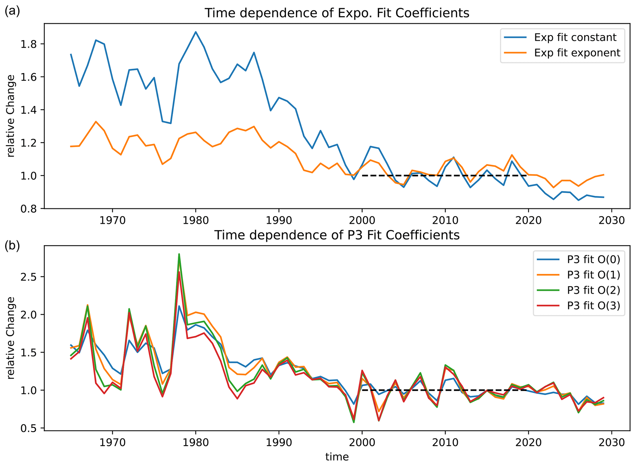
Figure 5 Time dependence of fit coefficients (a) for the exponential fit to effective lifetimes τ_eff and (b) with the third-order polynomial fit. All fit coefficients are normalized to the average over the years 2000–2019 (period indicated by the dashed line).

4.2 Application of correction schemes to model data

As the next step, we apply the correction scheme with different fits to model data to quantify how well the correction scheme is able to remove biases due to the chemical sinks in SF₆-based AoA. In the self-consistent model context, where we have the full information of ideal and apparent AoA, we can test whether the assumptions and fits made in the formulation of the correction scheme hold. In particular, we test how well different fit functions perform and how much the correction improves using latitudinally dependent fit coefficients instead of globally averaged ones.

We first present an example time series at mid-latitudes in the middle stratosphere (at 30 hPa and 46° N; see Fig. 6). Consistent with Loeffel et al. (2022), SF₆-derived apparent AoA increases over time, while the ideal AoA remains constant, as expected in the time slice simulation with constant climate. The difference between apparent AoA and ideal AoA is around 0.5 years in the year 2000 and up to 1 year towards the end of the simulation in 2030 (see Fig. 6). Corrections with exponential and third-order polynomial fits are performed, both with either latitude-dependent or global fit coefficients. All four methods are able to strongly reduce the difference between apparent and ideal AoA over the entire simulation period to less than about 0.15 years. All correction schemes overcorrect slightly before ∼ the year 2000, likely because of the change in effective lifetime over time in this period due to spin-up effects (see Fig. 5). Furthermore, the remaining difference between the corrected AoA and ideal AoA has a seasonal cycle, indicative of seasonal variations in the effective lifetime which are not captured by the annual mean fit coefficients. The correction using an exponential fit performs slightly worse than the correction using the third-order polynomial, but differences between the methods are small. There is almost no difference between the corrected AoA using global versus latitude-dependent fit coefficients at this location in the mid-latitude middle stratosphere.

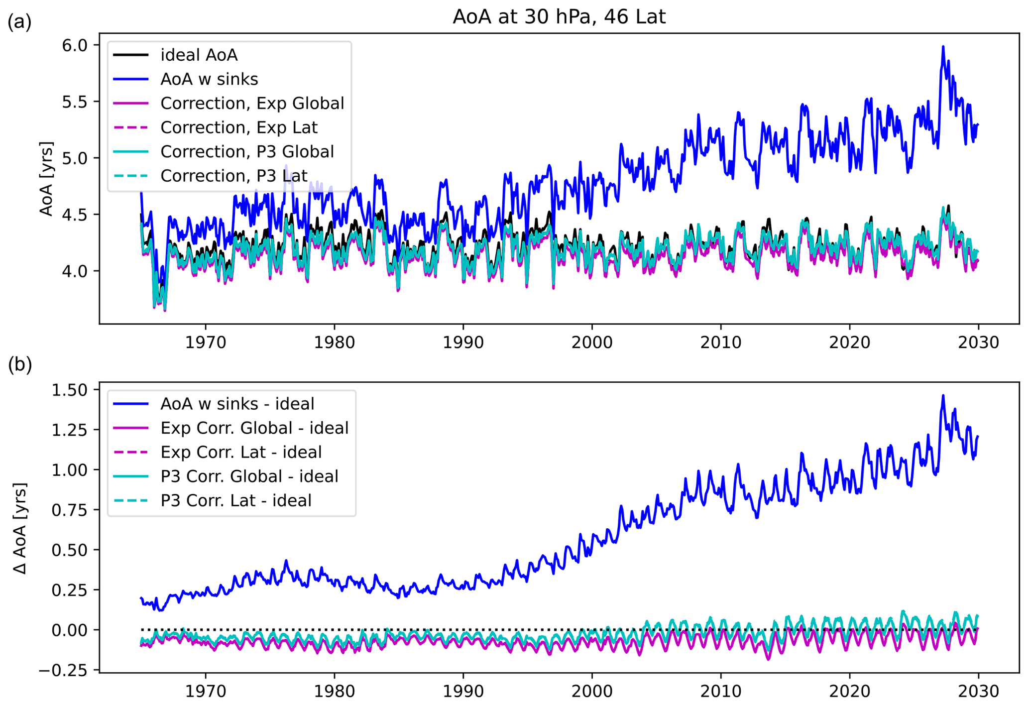
Figure 6 (a) Time series of ideal mean AoA (black) in mid-latitudes (46° N) and at 30 hPa together with apparent SF₆-based AoA (blue) and apparent AoA corrected with the exponential correction scheme (magenta) and the P3 correction scheme (cyan). (b) Same as above but showing differences from the ideal mean AoA.

The gain of applying the correction at each latitude and pressure level is demonstrated in Fig. 7 for corrections with the exponential and the third-order polynomial, each of them for global and latitude-dependent fit coefficients. For reference, the top panel in Fig. 7 shows the relative difference between apparent and ideal AoA for the uncorrected SF₆-derived AoA, showing average differences of 2 %–5 % for young air aged 1–2 years, differences between 5 % and 10 % for AoA between 2 and 4 years of age and strongly rising differences for older air. All correction methods are capable of reducing the relative difference below 2 % for AoA younger than 4 years in almost all regions of the stratosphere. The polynomial fit even reduces the relative differences to less than 1 % in almost all regions for ideal AoA of up to 5 years, in particular when using latitude-dependent fit coefficients. Above ideal AoA of 5 years, the bias in apparent AoA increases strongly. As can be seen in Fig. 3b, both the corrections based on the exponential and the linearly extrapolated polynomial fit (see discussion in Sect. 4.1) are for most seasons and latitude bands too conservative (i.e. undercorrect). Since the fits are performed only for ideal AoA below 5 years, the correction scheme is not designed to remove this bias for very old air completely.

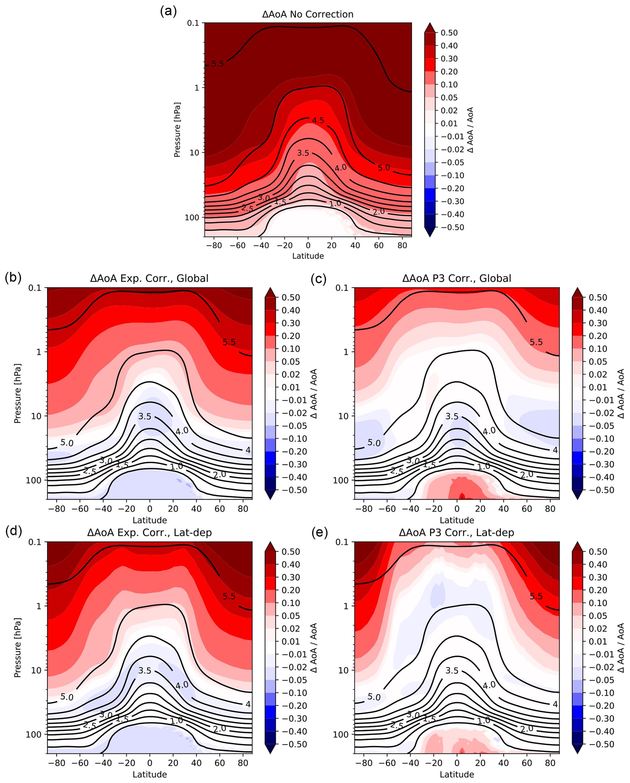
Figure 7 (a) Relative difference between apparent mean AoA and ideal mean AoA averaged over 2000–2009 without correction. Black contours show the climatology of ideal AoA in all panels. Panels (b), (c), (d) and (e) show the relative difference between apparent and ideal mean AoA as above but with the sink correction applied using (b, d) exponential and (c, e) third-order polynomial fits with either (b, c) global mean fit coefficients or (d, e) latitude-dependent fit coefficients. Note the non-linear colour bar.

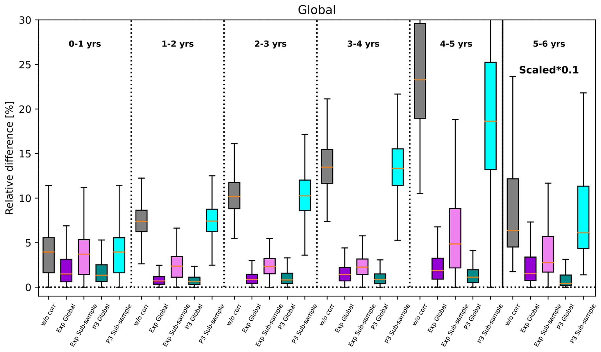
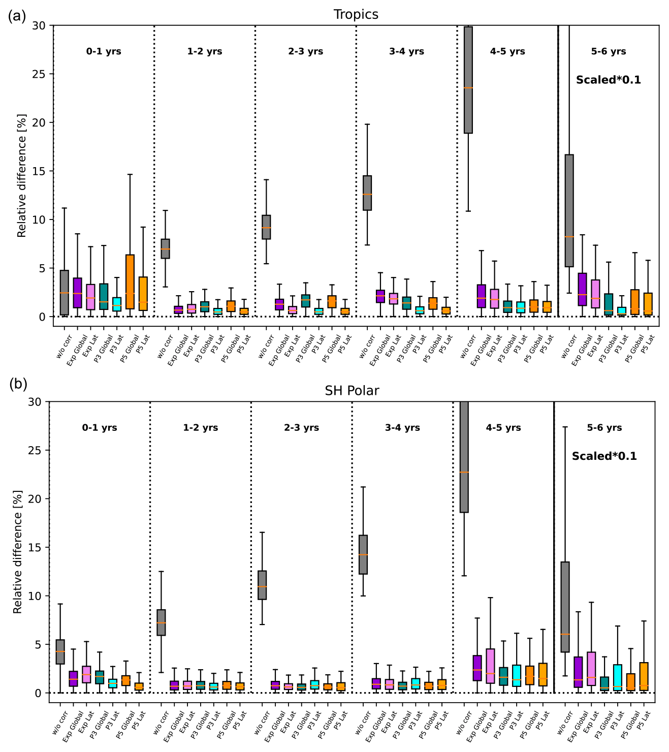
The reduction in biases in apparent AoA through the sink correction is further quantified in Fig. 8 for different AoA bins. The probability distributions of relative differences are based on monthly zonal mean data for the decade 2000–2009. The relative differences between apparent corrected and ideal AoA are strongly reduced compared to the uncorrected SF₆-derived AoA. This is true for all correction schemes. The improvement is smallest for AoA below 1 year, where the effects of sinks are small (median deviation of less than 5 %) and for which the correction scheme is not designed. Nevertheless, applying the correction scheme does not degrade AoA for those young air masses.

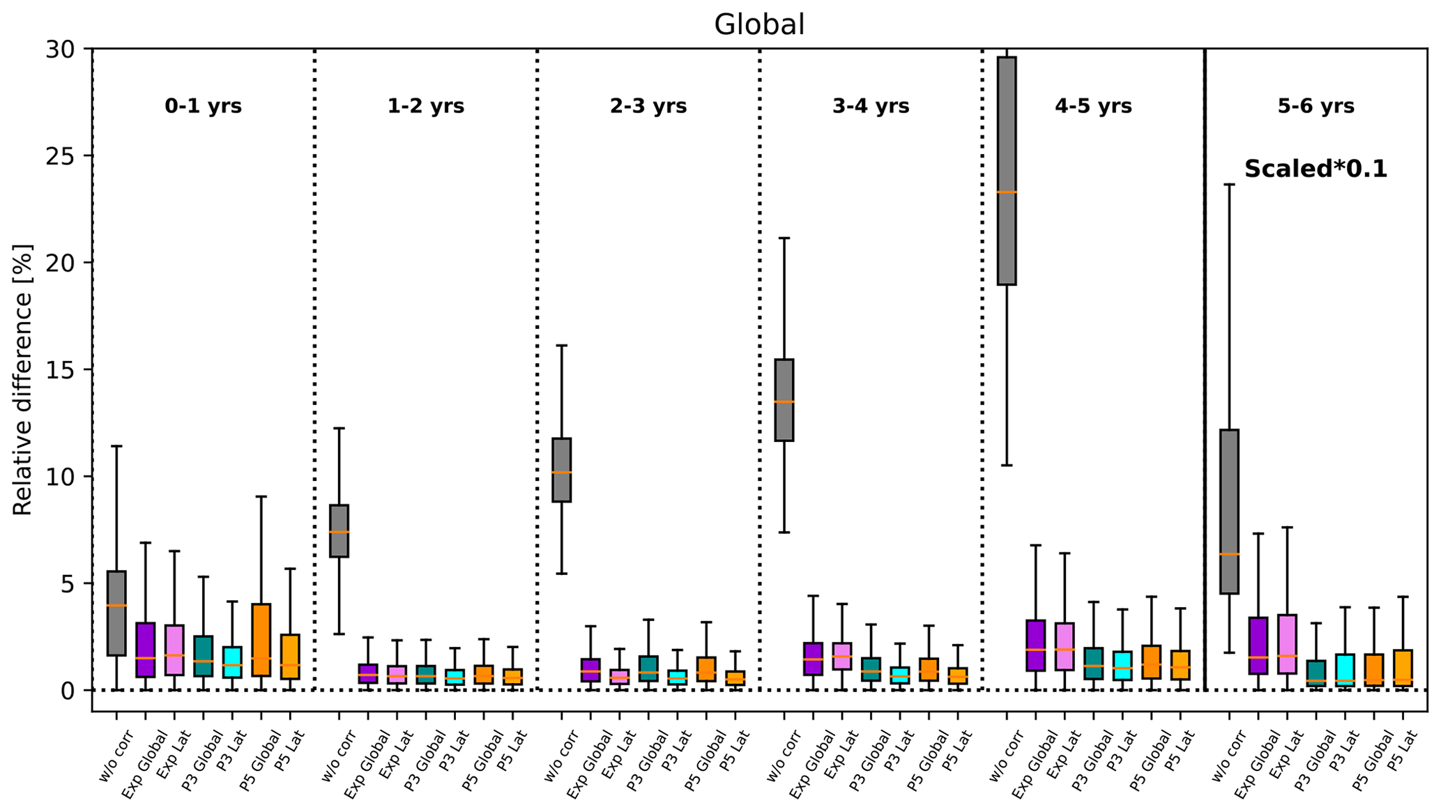
Figure 8 Relative differences between ideal AoA and apparent AoA without and with different correction schemes (see labels on the x axis) sorted by AoA for the years 2000–2009. Note that the values for AoA between 5–6 years are scaled by a factor of 0.1. For the first AoA bin of 0–1 year, AoA below 0.2 years is excluded to avoid excessive relative differences. The coloured boxes show the range of the lower to upper quartile of the data; the orange line is the median, and the whiskers indicate the minimum and maximum values.

All correction methods reduce the relative differences to below 1 % in the median for AoA between 1 and 3 years and to below 2 % for AoA up to 5 years. This corresponds to a factor of 10 or more compared to the median of relative differences for the uncorrected AoA. The polynomial fit methods perform slightly better than the exponential fit method in particular for AoA between 3 and 5 years, as is expected from the better ability to fit the effective lifetimes (see Sect. 4.1). There is little gain when moving from a third-order to a fifth-order polynomial fit. For AoA outside the range of 1–5 years, the fifth-order polynomial performed even more poorly, likely because outside the fit region higher-order polynomials are poorly constrained. Thus, based on those results we conclude that a third-order polynomial fit performs overall the best.

Using latitude-dependent fit coefficients versus global fit coefficients leads to slightly larger reductions in the relative AoA differences in particular for AoA of 2–3 years. The better performance of latitudinal fit coefficients stems mostly from tropical latitudes (see Fig. A1), where the effective lifetimes differ from the remaining latitudes in particular for AoA of 2–4 years (see Fig. 4).

For AoA beyond 5 years, relative differences between uncorrected apparent and ideal AoA become very large, exceeding 50 % in the median and reaching up to almost 250 % for extreme cases (note the scaled values for this AoA bin in Fig. 8). While the correction is not designed for this AoA range, it is still capable of reducing the relative difference from ideal AoA substantially. In particular, the polynomial fit reduces the median of relative differences to below 10 %. The latitude-dependent fit coefficients perform worse than the global fits for those old air masses, stemming from an undercorrection at high latitudes (see Figs. A1 and 7).

The fit coefficients show substantial changes for earlier time periods (see Fig. 5), but we use the average fit coefficients for 2000–2019 for all times. Despite this, the relative differences between SF₆-derived and ideal AoA can also be reduced in the 1980s data to below 2 % in the median for all ideal AoA ranges between 1 and 5 years and with all correction methods (not shown). However, the gain compared to uncorrected AoA is generally smaller since the effects of sinks on AoA are weaker in the 1980s data (ranging from 2 % to 9 % for AoA between 1 and 5 years).

The increasing effect of SF₆ sinks over time induces apparent positive trends in AoA (see Loeffel et al., 2022, and Fig. 9b). Since we use a time slice simulation, trends in ideal AoA are not significant (except a few locations, highlighting the role of natural variability). For the corrected SF₆-based AoA, trends are strongly reduced compared to the uncorrected apparent AoA trends and are mostly insignificant for AoA values below about 4 years. However, the correction scheme does not completely remove apparent trends; a weak significant trend remains in mid-latitudes in the lower stratosphere in particular. Also for AoA values above about 5 years, a significant positive trend remains, in particular for the exponential scheme. This is consistent with the AoA correction not being able to reduce the very strong biases for those very old air masses (see Fig. 7).

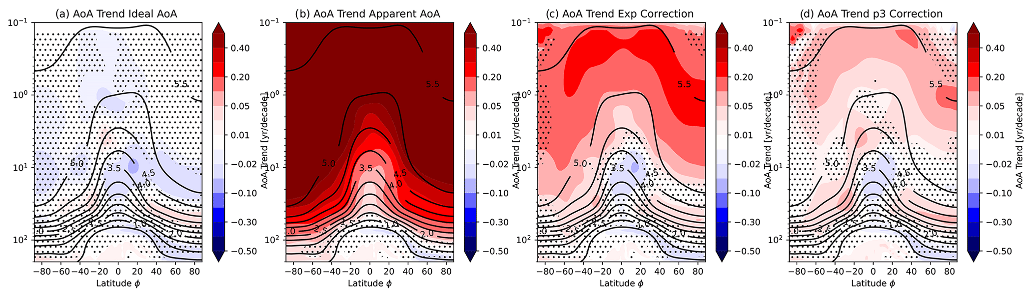
Figure 9 Linear trends in AoA over 1990–2020 in (a) ideal AoA, (b) apparent AoA and corrected AoA with the (c) exponential and (d) P3 scheme. Hatching indicates where trends are not significant at a 95 % level. Black contours display the ideal AoA climatology.

Furthermore, we investigate the effects of the sink correction scheme on the difference between tropical and mid-latitude AoA profiles. This is a useful diagnostic as it can be linked to the strength of the overturning circulation (e.g. Linz et al., 2017). The latitudinal age difference for the years 2000–2009 is displayed in Fig. 10, and ideal age shows the typical profile with the largest latitudinal differences in ideal AoA in the lower stratosphere around 60 hPa (e.g. Dietmüller et al., 2018). Apparent AoA strongly overestimates the AoA difference (by about 30 % at 60 hPa, increasing to more than 100 % above 10 hPa). The mass flux through a given surface is inversely related to the age difference between upwelling and downwelling regions on that surface (Linz et al., 2016), and so apparent age leads to a significant underestimate of the circulation strength throughout the stratosphere. The corrected AoA is able to remove this overestimation of the AoA difference. In particular, with the P3 correction, the AoA difference is reproduced remarkably well up to about 3 hPa. Interestingly, the latitude-dependent fit coefficients are not beneficial for the AoA difference diagnostic but perform as well as the correction schemes with global mean coefficients. This is consistent with small differences between corrected mean AoA with global versus latitude-dependent coefficients (of less than 5 %; see Fig. 7).

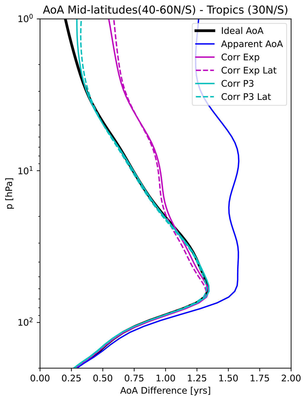
Figure 10 Mid-latitude (40–60° N/S) to tropical (30° N–30° S) AoA differences averaged over the years 2000–2009 for ideal (black), apparent (blue) and corrected AoA (cyan and magenta for third-order polynomial and exponential correction).

4.3 Subsampled data

In the previous sections, we examined the skill of the sink correction scheme when all model data are available for estimating the fit coefficients. However, the goal is to apply the sink correction to observational data and ideally constrain the coefficients for the correction based on observations. However, from observations we have much less information on the relation of “ideal” to apparent AoA. Therefore, we test here by how much the fits and the correction degrade if only limited and uncertain data pairs of ideal and apparent AoA are available to perform the fits on.

To do so, we select data from the model simulation representative of a limited number of observational data sets and choose data from 1 selected month and the latitude and height region of observations for each of the samples. We choose here 10 different data samples, representative of the observational data we have available for comparison (see Sect. 3.2 for a description of the data sets). The subsampled data are almost all located in the Northern Hemisphere, mostly in mid-latitudes with a few tropical and high-latitude profiles. Furthermore, only four profiles reach or are just above the height of 30 km; i.e. older air is underrepresented. The differences between apparent and ideal AoA for the subsampled data are shown in Fig. 11a. Due to the limited data, only one global fit is performed, since the data are not sufficient for latitude-dependent fits. However, as shown in the last section, using global instead of latitude-dependent fit coefficients does not degrade the correction significantly.

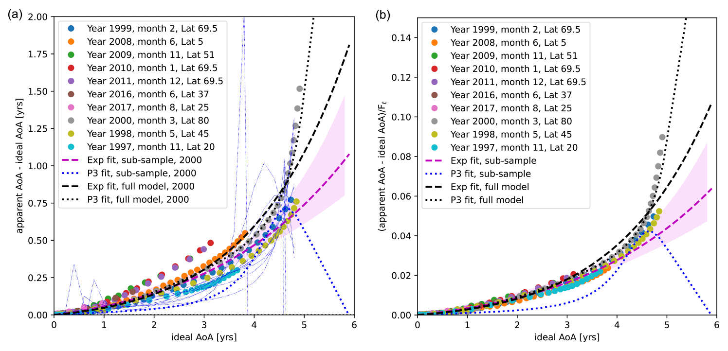
Figure 11 (a) Difference between apparent AoA and ideal AoA from model AoA data subsampled to a reduced data set representative of observational data availability. Shown are fit lines for full model data (black) and for subsampled data (magenta for exponential fit, blue for third-order polynomial fit). The violet shading indicated the uncertainty in the exponential fit to the subsampled data estimated via bootstrapping (see text). Uncertainty from the third-order polynomial fit is omitted as it spans the whole domain; instead, 10 randomly chosen example fit lines are shown (thin blue lines). (b) Same as the left panel but with the y axis normalized by F_t to remove the time dependence of the sink effect. Individual fit lines for the polynomial fit are omitted in this panel for clarity.

We perform a bootstrap procedure to estimate the uncertainty in the fit coefficients. Specifically, we choose 141 samples from the 141 available data points with replacements and add a random error drawn from a normal distribution with standard deviation of 0.1 years to each apparent and ideal AoA. This error is roughly representative of the uncertainty in observational data (see Sect. 3.2). We repeat this procedure 1000 times and calculate the average and standard deviations of the fit coefficients from this suite.

As seen in Fig. 11, the resulting fit line for the exponential fit to the subsampled data (magenta) lies below the fit based on the full model data (black). The fit varies moderately within 2 standard deviations, resulting in a correction at 5-year AoA spanning between about 0.65 and 0.95 years. The third-order polynomial fit, on the other hand, is very unconstrained for the subsampled data (dotted blue lines). The 2-standard-deviation range spans essentially the whole domain; therefore, only a few example fits are shown to demonstrate the unconstrained fit.

The effects of the uncertainty in the fit coefficients on the correction of AoA are summarized in the error statistics in Fig. 12. The correction was performed for fit coefficients plus and minus 2 standard deviations from its best estimate for the fits to the subsampled data. The probability distributions show relative differences including the corrections with both the fit coefficients plus and minus 2 standard deviations. The relative differences between ideal AoA and corrected AoA with the third-order polynomial fit are very large and span a wide range, which is consistent with the unconstrained fit lines found above. Thus, we conclude that correction with a third-order polynomial fit based on a limited amount of data and/or uncertain data is not advisable, as the coefficients are not well constrained. The exponential fit, on the other hand, is much more robust. The relative difference between corrected and ideal AoA is larger when using the exponential fit coefficients obtained from the subsampled data compared to the full model data for all AoA bins. Nevertheless, the correction still reduces the error compared to uncorrected data substantially (to below 5 % for AoA between 1–4 years and below 10 % for AoA between 4–5 years). In conclusion, despite the fact that limited information of the relation of SF₆-derived and ideal AoA leads to degraded fits, the correction scheme based on the global exponential fit is still very beneficial compared to using uncorrected SF₆-based AoA.

Figure 12 Same as Fig. 8 but contrasting correction with subsampled to full model data fit coefficients. The errors in correction with fits to subsampled data include fits with the average fit coefficient ±2 standard deviations.

5 Comparison and application to observational data

In Sect. 4, the performance of the correction scheme was carefully evaluated based on model data, and it was found that the schemes are highly beneficial to remove biases in SF₆-based AoA estimates. However, this was entirely based on model data, and one can question whether the chemical sink of SF₆ is constrained well enough in the model to trust the derived coefficients. Ideally, we would perform similar fits between AoA derived from observed SF₆ and from simultaneous observations of other age tracers that do not suffer from the sinks. However, as we will show in the following section, available observational data are currently not able to constrain the fit parameters well enough. Instead, we will show that the model-derived correction fit lines lie within the bounds given by observations, and we will test the performance of the correction with model-based parameters on independent AoA observations.

We use the observational data sets described in Sect. 3.2 from a number of aircraft campaigns and balloon flights. Figure 13a shows differences between SF₆-based AoA and AoA based on the alternative tracers as a function of the latter, which is similar to what is shown in Fig. 4a but for observational data. It is immediately clear from this figure that observations show a large spread in the difference between SF₆ and alternative-tracer-based AoA. In the left panel, the difference is compared to model data sampled in the same month and years as when the observational campaigns took place. The model data are still monthly and zonal mean profiles, explaining the much-reduced variability compared to observational data. Furthermore, note that the meteorological conditions in the free-running model do not of course match the observed state of the atmosphere, so the sampling is rather meant to capture variations due to the latitude, season and the underlying trend in SF₆. Generally, the model data are found to lie within the large scatter of observational data for mean AoA below about 5 years. One high-latitude balloon flight sampled air within the polar vortex (Ray et al., 2017) with CO₂-based mean AoA between 5 and 6 years. For this profile, the difference in CO₂- and SF₆-based AoA increases strongly to up to 4 years. The AoA differences in the model from a similar latitude band and month as this balloon flight show a similarly strong increase but occurring already at younger ideal mean AoA values.

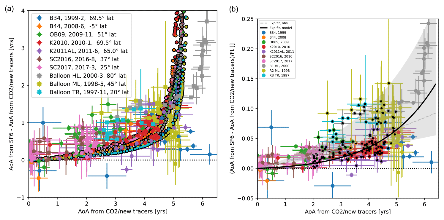
Figure 13 (a) Difference between apparent SF₆-based AoA and AoA derived from alternative age tracers for a number of aircraft and balloon measurements (see legend). Monthly and zonal mean model data for the same latitude bands and months are shown in the same colour but with a black circle. (b) Same as (a) but with the y axis normalized by the function F_t(t) to adjust for different years of observations. The exponential fit based on all model data is shown in black, and the fit based on chosen observations (indicated with black dots) is shown in grey with uncertainty shaded grey.

The measurement campaigns took place during different years within a 21-year period (between 1997 and 2017), so the effect of the sinks increased over this time frame. To eliminate this time dependence, the age differences are normalized by the time-correction function F_t (see Sect. 2), and the resulting data points are shown in Fig. 13b. The scatter is somewhat reduced compared to the uncorrected differences on the left but is still substantial. Attempts to fit the parameters for the correction scheme result in a very large uncertainty. In particular for young AoA values below 2 years, some measurements indicate already a large difference from SF₆-based AoA ranging between 0 and 1 year (see Fig. 13a). This might partly be due to local influence close to sources of the alternative AoA tracers, potentially leading to biases in the estimate of ideal AoA from alternative tracers and/or SF₆-based AoA (Adcock et al., 2021). In Sect. 4.3, we find that the subsampled model data on the availability of observational data are not able to constrain the third-order polynomial fit. Therefore, we only use the exponential fit method in the following section, both for attempts to fit coefficients based on observations and for any corrections of the observational data. When discarding all mean AoA values below 2 years and above 5 years, the exponential fit for the correction scheme as displayed in grey in Fig. 13b is obtained (based on a bootstrapping algorithm to estimate the uncertainty; see the grey shading). However, the fit is very sensitive to including or excluding individual data points. When including data for values between 1 and 2 years, the resulting fit would indicate an increase in the effective lifetime with mean AoA, which can be ruled out as non-physical. Therefore, we have to conclude that the currently available observational data that allow for an estimation of SF₆-based AoA and AoA from an alternative tracer are not sufficient in quantity and quality to constrain the fit parameters for the sink correction.

Instead, we have to rely on the model-based parameters for the correction scheme. The model-based global mean correction curve for the exponential fit is included in Fig. 13b (black curve). While the large scatter of observations does not allow for a detailed evaluation, we find that the model-based correction scheme lies within the observational uncertainty. Therefore, we suggest at this stage that the best practice is to apply the sink correction with the model-based parameters. While fit functions which are of higher order than the exponential fit and the latitude-dependent fit coefficient did lead to a slightly better performance of the correction within the model (see Sect. 4.2), we rather use the more conservative exponential fit and the global mean fit parameters in the following to correct observational data. This is, on the one hand, because of the larger sensitivity in the polynomial fits (see Sect. 4.3) and, on the other hand, because we want to reduce model-dependent information. In particular, the latitude dependence of fit coefficients likely is a function of the representation of circulation in the model (e.g. location and strength of the polar vortex), while we assume the global fit to be less sensitive to the representation of circulation in a particular model. Comparisons to other independent observational data and inter-comparisons with other models with the implementation of chemical sinks of SF₆ should be performed in the future to better constrain the fit coefficients of the sink correction.

The correction scheme with the model-derived parameters is applied to in situ and satellite data presented in Fig. 14. The latitudinal profiles of in situ mean AoA data compiled by Andrews et al. (2001) at around 20 km consist of AoA both based on CO₂ and based on SF₆. The SF₆-based mean AoA data consistently lie above AoA based on CO₂, in particular for mid- to high latitudes. This difference is not necessarily caused only due to the chemical SF₆ sink, but also by the different temporal slopes and seasonality of the tracers time series, affecting the derivation of mean AoA (see e.g. Andrews et al., 2001; Bönisch et al., 2009).

When applying the sink correction to the SF₆-based mean AoA values, this consistent high bias of SF₆-based mean AoA is strongly reduced. In particular at northern mid- to high latitudes, CO₂- and SF₆-based AoA agree extremely well after the sink correction is applied, with the mean difference between CO₂ and SF₆ AoA for latitudes of > 40° being reduced from 0.43 to 0.03 years. In the Southern Hemisphere, the scatter is larger due to generally poorer data quality. Nevertheless, the bias between CO₂- and SF₆-based AoA is also reduced from 0.33 to 0.13 years for latitudes south of 40° S.

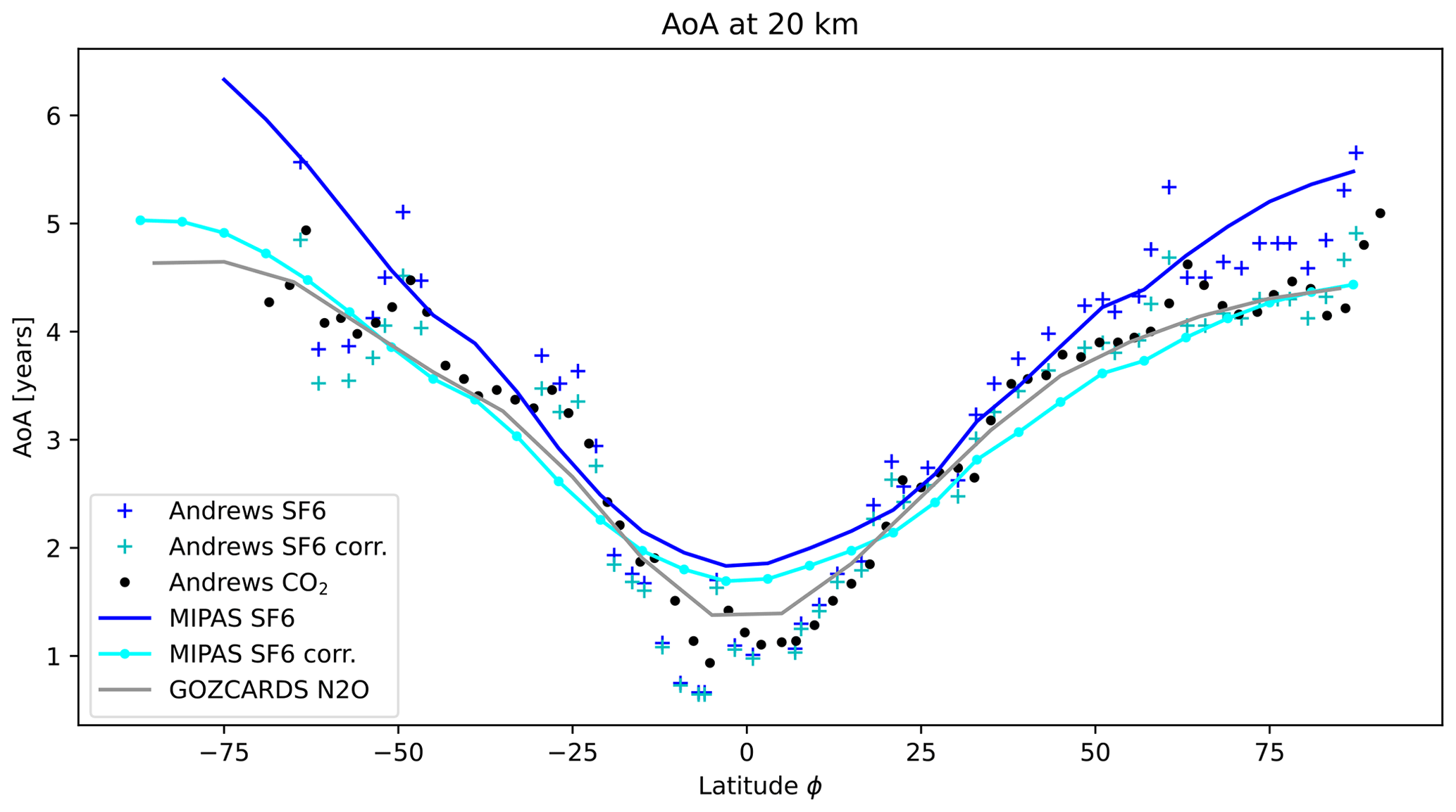
Figure 14 Observational mean AoA data at 20 km altitude from in situ observations by Andrews et al. (2001) based on CO₂ (black dots) and SF₆ original estimates (dark-blue crosses) and with the sink correction applied (light-blue crosses). Mean AoA from MIPAS derived from SF₆ (Stiller et al., 2021) and averaged over the whole data record is shown as a solid dark-blue line and the sink-corrected values as a solid light-blue line. Mean AoA derived from GOZCARDS N₂O (Linz et al., 2017) and averaged over the entire record is shown as a solid grey line.

Furthermore, the latitudinal climatological profile of AoA around 20 km is shown for two satellite products, SF₆-based mean AoA from MIPAS (Stiller et al., 2021, and see Sect. 3.2) and AoA derived from N₂O measured by Aura MLS and ACE-FTS (the GOZCARDS data product; see Sect. 3.2). The SF₆-based mean AoA from MIPAS is older compared to AoA based on N₂O and in situ CO₂ observations, in particular at high latitudes, but agrees well overall with the in situ SF₆-based mean AoA. After applying the sink correction to the MIPAS AoA data, agreement between MIPAS AoA and the non-SF₆-based AoA data sets is much improved, in particular at high latitudes. At mid-latitudes, corrected MIPAS mean AoA is slightly lower than the other estimates, while in the tropics the high bias is only slightly reduced.

Overall, mean AoA estimates from different trace gases and from different observational sources agree much better after applying the SF₆ sink correction. This provides further evidence that the sink correction is a promising way forward to remove biases in mean AoA estimated based on SF₆.

6 Summary and conclusion

In this paper, we have developed a correction scheme for SF₆-based AoA to remove the biases generated by chemical SF₆ sinks. The correction scheme is based on a simplified formulation derived from the theory that provides a relation of ideal to apparent AoA dependent on (1) a time-dependent function of the reference SF₆ surface mixing ratio (which would be a linear function for a linear reference time series) and (2) the path-integrated average effective lifetime based on AoA. For the former, we suggest a simplified approximation based on the linearized reference time series. For the latter, we parameterize the effective lifetime as a function of ideal AoA. Based on global model data, we find that either an exponential or a third-order polynomial fit is suited for this parameterization. While the third-order polynomial fit captures the details of the AoA dependency of the effective lifetime better, it comes at the cost of high parameter sensitivity to uncertainty in the underlying data. Furthermore, we find that using latitude-dependent coefficients for the parameterization of the effective lifetime as a function of ideal AoA is beneficial, but the overall ability to reduce biases in SF₆-based AoA is only marginally improved. In the model, the simplified sink correction with global mean fit coefficients is able to reduce the biases in AoA by a factor of 5 to 10 to, on average, less than 2 % relative to ideal AoA for AoA values below 5 years. For AoA above 5 years, the relation between ideal and apparent AoA becomes weaker, and, therefore, the correction is not designed for those high ages above 5 years. Nevertheless, correcting AoA with the extrapolated fit lines for this AoA range also substantially reduced the bias. In addition to mean AoA, we showed that the correction scheme is able to remove apparent AoA trends in the lower stratosphere. Furthermore, the sink correction is able to correct the age difference between tropics and mid-latitudes, a diagnostic of the residual circulation strength, even when based on global mean fit coefficients. This is a promising result to enable more confident estimates of the circulation from SF₆ satellite data, which previously was limited only to the lower stratosphere (Linz et al., 2017).

In conclusion, the sink correction scheme performs very well within the self-consistent “model world” with all information available. However, how useful is this scheme to correcting observational AoA estimates given imperfect knowledge of the ideal to apparent AoA relationship? Firstly, we approach this question by subsampling the model data leading to erroneous fit coefficients. When using the less sensitive exponential fit function for the relation of the effective lifetime to AoA, we could show that despite incomplete knowledge and thus uncertain fit coefficients, the sink correction is able to reduce the AoA biases in all cases. In other words, even applying the sink correction with uncertain parameters is better than not applying any corrections. Of course this statement hinges on staying within a certain range of fit uncertainty; if the sink in the model were completely different than the real world, this would naturally not hold. The total stratospheric and mesospheric lifetimes of SF₆ estimated in the EMAC model simulations spanning 1900 years fall within the range of values provided by previous model and observational studies (e.g. Ray et al., 2017; Kovács et al., 2017; Kouznetsov et al., 2020, all providing ranges between around 800 and 3000 years), indicating the validity of EMAC's SF₆ depletion mechanisms despite existing uncertainties in lifetime determination (see also discussion in  Loeffel et al., 2022). Furthermore, comparisons of the model fit to available observational data of SF₆-based AoA and AoA deduced from CO₂ or the new alternative AoA tracers (Leedham Elvidge et al., 2018) indicate that the model sinks do lie within the observational spread. The spread is high, however, likely because of two reasons. Firstly, AoA deduced from realistic tracers is generally error-prone due to uncertainty in the reference time series and the non-linearity therein (including the seasonal cycle, in particular for CO₂) and, for example, the influence of local sources of the tracers. Those factors induce the large error bars in observational AoA (seen in Fig. 13). Secondly, the observational data used here are point measurements, while in the model we used monthly mean and zonal mean data. While the averaged data fall on the compact relationship between ideal AoA and apparent AoA, point data might differ from this line due to local mixing between different air masses (as is well-known for tracer–tracer relationships; see e.g. Plumb, 2002). It is not clear how strong the contribution of those two factors is to the large spread in the observed relationship between SF₆-based AoA and AoA from other tracers. If the contribution from internal variability by mixing is substantial, this would imply that the compactness of the relationship between SF₆-AoA and ideal AoA is limited for point measurements, and thus a correction is not easily possible. Until this issue is clarified, we recommend using the sink correction scheme on averaged data (over time periods of a month or so and/or large regions). Application of the sink correction to satellite and compiled in situ data confirms that the correction is able to reduce the discrepancy between different AoA estimates. In situ SF₆- and CO₂-based AoA values agree very well after the correction is applied, and the SF₆-based AoA deduced from MIPAS satellite observations agrees well with the N₂O-based AoA from the merged GOZCARDS satellite product when the correction is applied. Note, however, that AoA derived from N₂O also bears uncertainties; AoA is calculated from the N₂O–AoA relationship based on specific concurrent observations of N₂O and CO₂ in the northern mid-latitudes (see Sect. 3.2), and improved quantification of the latitudinal and temporal variations in the N₂O–AoA relation will be necessary to more reliably derive mean AoA by this method.

Overall, we conclude that observational data are currently not able to constrain the parameters for the sink correction scheme proposed here. Until this is possible, we recommend using the model-based global mean exponential fit parameters for the sink correction. While the model might be subject to biases, we could demonstrate that the relation of ideal to apparent AoA from the model lies within observational uncertainty and that the application of the model-based sink correction is successfully reducing differences in observational AoA estimates. However, future work is needed to test and better constrain the parameters for the sink correction scheme and to generally enhance our knowledge on the chemical sinks of SF₆ in the atmosphere.

Appendix A: Error statistics for tropics and high latitudes

In addition to the global statistics of the effects of the sink correction on the apparent–ideal AoA difference, in Fig. A1 those error statistics are presented in the same manner for AoA only in the tropics (20° S–20° N; Fig. A1a) and only in southern high latitudes (60–90° S; Fig. A1b).

Figure A1 Same as Fig. 8 but for individual regions: (a) tropics (20° S–20° N) and (b) SH high latitudes (60–90° S). Northern high latitudes show very similar results to the SH high latitudes (not shown).