Evaluation of downward and upward solar irradiances simulated by the Integrated Forecasting System of ECMWF using airborne observations above Arctic low-level clouds

The simulations of upward and downward irradiances by the Integrated Forecasting System (IFS) of the European Centre for Medium-Range Weather Forecasts are compared with broadband solar irradiance measurements from the Arctic CLoud Observations Using airborne measurements during polar Day (ACLOUD) campaign. For this purpose, offline radiative transfer simulations were performed with the ecRad radiation scheme using the operational IFS output. The simulations of the downward solar irradiance agree within the measurement uncertainty. However, the IFS underestimates the reflected solar irradiances above sea ice significantly by −35 W m⁻². Above open ocean, the agreement is closer, with an overestimation of 28 W m⁻². A sensitivity study using measured surface and cloud properties is performed with ecRad to quantify the contributions of the surface albedo, cloud fraction, ice and liquid water path and cloud droplet number concentration to the observed bias. It shows that the IFS sea ice albedo climatology underestimates the observed sea ice albedo, causing more than 50 % of the bias. Considering the higher variability of in situ observations in the parameterization of the cloud droplet number concentration leads to a smaller bias of −27 W m⁻² above sea ice and a larger bias of 48 W m⁻² above open ocean by increasing the range from 36–69 to 36–200 cm⁻³. Above sea ice, realistic surface albedos, cloud droplet number concentrations and liquid water paths contribute most to the bias improvement. Above open ocean, realistic cloud fractions and liquid water paths are most important for reducing the model–observation differences.

1 Introduction

The Arctic climate has changed more rapidly than the rest of the globe during recent decades. One clear sign is the reduction in the sea ice extent of the Arctic Ocean, particularly in September every year (Serreze and Meier, 2019). Another indicator is the increase in the near-surface air temperature in the Arctic, which is more than twice as large as for the whole globe (Rantanen et al., 2022; Wendisch et al., 2023). The ongoing changes of the Arctic climate system emphasize the need for adaptations of forecast models to Arctic-specific particularities (Jung et al., 2016). Improved prediction systems for the Arctic would be not only a direct benefit for the Arctic of the future with new shipping routes (Smith and Stephenson, 2013), but also an indirect benefit for forecasts in Northern Hemisphere midlatitudes at longer lead times. This is due to the link between the Arctic and the midlatitudes that was investigated by, e.g., Jung et al. (2014), Cohen et al. (2014), Overland et al. (2015) and Lawrence et al. (2019).

Numerical weather prediction (NWP) models, such as the Integrated Forecasting System (IFS) by the European Centre for Medium-Range Weather Forecasts (ECMWF), often appear more uncertain in the Arctic compared to other regions of the globe (Bauer et al., 2016). The reasons for the lower predictive skills in the Arctic are various and often linked to the particularities of the Arctic climate system. One obvious issue in the Arctic is the sparse observational coverage, which limits data assimilation (Bauer et al., 2016; Jung and Matsueda, 2016; Lawrence et al., 2019; Ortega et al., 2022). Furthermore, modeling of the sea ice cover is a major obstacle in correctly representing the Arctic surface energy budget, but is still uncertain due to the complexity of sea ice dynamics (Day et al., 2022). The representation of low-level Arctic clouds and especially mixed-phase clouds has been identified as another major source of uncertainty (Forbes and Ahlgrimm, 2014). As shown by Morrison and Pinto (2006), cloud microphysical schemes in particular cause uncertainties in the cloud phase and precipitation.

Low-level clouds occur frequently in the Arctic (e.g., Eastman and Warren, 2010; Mioche et al., 2015) and show a pronounced longevity above sea ice and open ocean (Shupe et al., 2006; Verlinde et al., 2007). Their radiative properties are controlled by a complex system of coupled microphysical and dynamical processes that may differ depending on the surface conditions (Morrison et al., 2012; Wendisch et al., 2019). Especially for optically thin clouds, with a liquid water path (LWP) less than 30 g m⁻², the cloud radiative effect changes significantly for only small changes of cloud properties (Shupe and Intrieri, 2004). Thus, these clouds potentially introduce major model uncertainties. To constrain the effect of Arctic low-level clouds on the atmospheric radiation budget, it is necessary to identify shortcomings of microphysical parameterizations in NWP models to properly predict snow rate and cloud properties (Solomon et al., 2009). A substantial underprediction of the cloud LWP together with an overprediction of the cloud ice water path (IWP) was revealed by Solomon et al. (2009), which indicated an unrealistic growth of ice particles in the Weather Research Forecast model. Solomon et al. (2023) showed that contemporary models have difficulties to represent the radiative impact of Arctic clouds and still struggle to keep liquid water at low temperatures. Additionally, the change in the surface type (sea ice or open ocean) when clouds move on or off the sea ice initiates air mass transformations and changes in the cloud dynamics. This transition can result in cloud formation or cloud dissipation and is still poorly represented in NWP models (Pithan et al., 2018; Wendisch et al., 2021).

Two different concepts to evaluate clouds and their radiative effects in NWP have been applied in the past. The first approach applies model inter-comparisons (e.g., Klocke and Rodwell, 2014) to identify model uncertainties. This technique is not able to quantify potential model biases compared to reality. The second approach makes use of observed cloud properties. This approach was applied in the past few decades to evaluate the representation of clouds in global NWP models using ground-based long-term cloud observations within the framework of Atmospheric Radiation Measurement (ARM) sites (e.g., Yang et al., 2006; Morcrette et al., 2012) or within the Cloudnet (Illingworth et al., 2007) framework (e.g., Hogan et al., 2009; Sinclair et al., 2022). Due to the nature of observations at a fixed location, only a few of these studies target specific Arctic sites (e.g., Klein et al., 2009; Morrison et al., 2009; Zhao and Wang, 2010; Forbes and Ahlgrimm, 2014). For an evaluation of the cloud representation in the central Arctic over the Arctic Ocean, satellite observations can be used, which provide a spatially broader view and in polar regions are associated with frequent overpasses by polar-orbiting satellites, but they cause difficulties in the data assimilation of microwave soundings above sea ice (Lawrence et al., 2019). Compared to the long-term observations of ARM, Cloudnet and satellites, shipborne observations provide short-term observations covering different slowly varying locations. Airborne observations bridge the gap between ground-based or shipborne observations and satellite observations and can provide in situ observations of cloud particle properties.

Efforts in the past to improve model representations of Arctic clouds covered diverse aspects and quantities. The parameterization and representation of the sea ice albedo in various models was evaluated by, e.g., Liu et al. (2007) and Karlsson and Svensson (2013), who identified the model sea ice albedo to determine both the sign and the amount of its cloud radiative effect. Low-level cloud fractions were assessed in reanalyses by Walsh et al. (2009) and were found to be underestimated in summer, which leads to a bias in the solar radiation flux, while Sotiropoulou et al. (2016) evaluated the improvement in the representation of the vertical structure of mixed-phase clouds in IFS by changing from a diagnostic to a prognostic parameterization of mixed-phase clouds. Integrated microphysical quantities such as LWP and IWP were investigated by Gu et al. (2021), who evaluated these quantities in Arctic reanalyses and found a mean underestimation of both LWP and IWP over the Arctic region compared to satellite observations. The representation of cloud droplet number concentrations in different models was evaluated by Geoffroy et al. (2010), Brenguier et al. (2011) and McCusker et al. (2023), who showed a slight improvement in the overestimation of the liquid cloud mass mixing ratio in low-level clouds in the Met Office Unified Model (UM) by using representative cloud droplet number concentrations. Stevens et al. (2018) concluded from their model intercomparison of cloud condensation nuclei-limited tenuous Arctic clouds that an appropriate treatment of the cloud droplet size distribution within models is important in order to account for aerosol–cloud interactions. Regarding the IFS, Beesley et al. (2000) evaluated the ECMWF model with observations collected during the Surface Heat Budget of the Arctic Ocean (SHEBA) campaign (Uttal et al., 2002) and identified a much larger observed fraction of liquid water clouds. Tjernström et al. (2021) examined the IFS with observations from the Arctic Ocean 2018 (AO2018) expedition (Vüllers et al., 2021) and revealed too high (near-)surface air temperatures in the IFS. McCusker et al. (2023) evaluated clouds during AO2018 within the IFS that overestimated cloud occurrence below 3 km. Forbes and Ahlgrimm (2014) revealed an underestimation of IFS cloud top albedo compared to observations from the Clouds and the Earth's Radiant Energy System (CERES) project. The bias is linked to an underestimation of liquid water content (LWC) near cloud tops, which results from the parameterization of the cloud phase based on diagnostic air temperature.

However, these evaluations are often based on remote sensing products, which themselves include major uncertainties mostly resulting from several assumptions in the retrieval algorithm, e.g., viewing geometries, instrument sensitivity or the ice crystal shape (Wendisch, 2005). Therefore, Formenti and Wendisch (2008) recommended comparing NWP models in the observational space of radiation, e.g., solar and thermal infrared radiation, radar and lidar reflectivities. Huang et al. (2017) used this approach to evaluate different global reanalyses such as the ECMWF Reanalysis–Interim and the Climate Forecast System Reanalysis by the National Centers for Environmental Prediction, while Matsui et al. (2014) and Berry et al. (2019) suggested evaluating Earth system models. Observations of airborne solar spectral irradiance have been used by Wolf et al. (2020) in combination with along-track radiative transfer simulations of the operational ecRad radiation scheme of ECMWF and a benchmark radiative transfer model. Their analysis indicated that IFS underestimates the ice water content (IWC) in a frontal cloud system close to Iceland and that differences in the absorbing spectral band indicate deficiencies in the ecRad ice crystal optical properties. For the Arctic CLoud Observations Using airborne measurements during polar Day campaign (ACLOUD; Wendisch et al., 2019), Kretzschmar et al. (2020) applied similar measurements and found a pronounced underestimation of the negative cloud radiative effect in the ICON model. This bias was traced back to the cloud condensation nuclei activation in the microphysical scheme. For a specific cloud case observed during ACLOUD, Ruiz-Donoso et al. (2020) investigated the thermodynamic phase of mixed-phase clouds as modeled by ICON large-eddy simulations and found that measured spectral radiances reveal an underestimation of the modeled ice crystal number concentration. Jäkel et al. (2019b) used ACLOUD observations to analyze the performance of the sea ice albedo scheme used in a regional coupled climate model and found an underestimation of the variability of the sea ice albedo caused by a biased surface albedo parameterization dependence on surface temperature. So far, the comprehensive ACLOUD data set has not been used for any IFS evaluation. While efforts have been made to include sea ice dynamics in IFS to tackle the high sea ice variability close to the sea ice edge (Keeley and Mogensen, 2018), the sea ice albedo in IFS is still based on climatological values with shortcomings identified by Pohl et al. (2020) using satellite observations.

In this paper, airborne radiation data from the ACLOUD campaign are used to evaluate the representation of Arctic low-level clouds and sea ice albedo in the IFS. The comparison is based on the observational space of solar irradiance and additionally implements active cloud remote sensing and in situ cloud microphysical observations. Section 2 describes the comparison strategy of the observations and radiative transfer simulations, which are analyzed in Sect. 3. Based on the additional measurements, a sensitivity study is presented in Sect. 4. It aims at reducing the differences between modeled and observed irradiances by improving the surface albedo, cloud fraction and macro- and microphysical properties (LWP, IWP and cloud droplet number concentration) with the actually measured data. The contributions of each individual parameter to the overall model uncertainty are summarized in the Conclusions in Sect. 5.

2 Data and methods

2.1 Airborne observations

Airborne observations of the ACLOUD campaign (Ehrlich et al., 2019), which took place in May/June 2017 around Svalbard, Norway, provide a comprehensive data set of in situ and remote sensing observations for model evaluation and were used in this analysis. Two upward- and downward-looking CMP22 pyranometers (spectral range of 300–3000 nm) aboard the Polar 5 aircraft (Wesche et al., 2016) measured the broadband solar irradiance (Stapf et al., 2019), which is referred to as “solar irradiance” in this study. The uncertainty of the CMP22 irradiance is typically about 2 % according to characterizations by Vuilleumier et al. (2014) for ground-based operations. However, the airborne operation of the CMP22 in Arctic conditions may increase these uncertainties depending on the solar zenith angle and environmental conditions, as described by Ehrlich et al. (2023) on a high-altitude aircraft and by Su et al. (2008) in a laboratory study, and on active stabilization performance (Wendisch et al., 2001). The data are corrected for the aircraft-specific operation, as summarized in Ehrlich et al. (2019), including corrections for aircraft attitude and instrument inertia. For the conditions during ACLOUD, a maximum uncertainty of 3 % in regular straight flight sections is assumed.

Spectral solar irradiances are measured on Polar 5 with the Spectral Modular Airborne Radiation measurement sysTem (SMART; Jäkel et al., 2019a; Wendisch et al., 2001) covering the spectral range between 345 and 2150 nm with a spectral resolution of 3–15 nm (Ehrlich et al., 2019). Additional remote sensing observations aboard Polar 5 include the Airborne Mobile Aerosol Lidar (AMALi) system (Stachlewska et al., 2010) and the Microwave Radar/radiometer for Arctic Clouds (MiRAC; Kliesch and Mech, 2019; Mech et al., 2019). AMALi is sensitive to both liquid and ice layers, while MiRAC is particularly sensitive to ice layers in the clouds. The cloud top altitude is derived from AMALi using a robust backscatter gradient approach that is retrieval independent and is only based on the instrument threshold chosen (Kulla et al., 2021). For MiRAC a threshold of −30 dBZ equivalent reflectivity factor is applied to identify cloud particles above the height of 150 m. Altitudes below that were not considered so as to exclude ground clutter. The uncertainty of the radar detector is given by Mech et al. (2019) as 0.5 dBZ, which only slightly affects the uncertainty in detecting cloud layers.

The Polar 6 aircraft was equipped with numerous in situ cloud probes. This study makes use of cloud particle number concentrations measured by the Small Ice Detector Mark 3 (SID-3; Schnaiter and Järvinen, 2019; Hirst et al., 2001; Vochezer et al., 2016). To characterize the surface conditions, sea ice concentration satellite data are retrieved from the Advanced Microwave Scanning Radiometer 2 (AMSR2) measurements (Melsheimer and Spreen, 2019; Spreen et al., 2008).

2.2 Radiative transfer simulations

2.2.1 Integrated Forecasting System

The results of the simulations presented in this paper have been achieved with the “Atmospheric Model high resolution” configuration (HRES) of the IFS of the ECMWF. Model cycle 43r1 was operational during the time of ACLOUD. A detailed description of the IFS can be found at https://www.ecmwf.int/en/publications/ifs-documentation (last access: 20 March 2024). To evaluate the short-term forecast and not the model initialization, the 00:00 UTC runs with hourly forecast steps are used, issued about 12 h before each flight. Prognostic variables from the IFS are available at 137 model levels. Approximately 32 levels lie below a typical flight altitude of 3000 m, with the highest vertical resolution of about 30 m close to the ground. The spacing between grid points of the longitude–latitude grid is 0.07° both along the longitude and the latitude axis, resulting in a horizontal resolution of 1.4–7.8 km in the campaign region. The surface type is classified as open ocean or sea ice when the sea ice concentrations by AMSR2 and IFS are below 0.01 % or above 60 %.

2.2.2 ecRad radiation scheme

The prognostic variables air pressure, air and skin temperature, specific humidity and cloud fraction from the IFS serve as direct input to the ecRad radiation scheme (Hogan and Bozzo, 2018). The ecRad version 1.4.0 is applied in an offline mode, which allows sensitivity studies to be run. In addition, the required quantities of liquid or ice cloud mass mixing ratios are calculated as sums of specific cloud liquid or ICW and specific rain or snow water content. Similarly, the effective radii are not prognostic variables in the IFS and need to be calculated consistently to the IFS. The definition of ice cloud effective radius follows the parameterization by Sun and Rikus (1999) and Sun (2001). The definition of liquid cloud effective radius in the IFS is based on the parameterization by Martin et al. (1994) with an adjustment by Wood (2000).

Over open ocean the IFS distinguishes between a spectrally constant surface albedo value of 0.06 for diffuse radiation and a solar zenith angle-dependent surface albedo given by Taylor et al. (1996) for direct radiation. Here, the open ocean albedo is approximated with the diffuse albedo only. The surface albedo used in ecRad is composed of this open ocean albedo and the sea ice albedo, which is based on the one-dimensional sea ice model by Ebert and Curry (1993) providing a monthly mean climatology of the spectral surface albedo in six solar bands (boundaries at 0.185, 0.250, 0.440, 0.690, 1.190, 2.38 and 4.0 µm). This climatology is interpolated to the day of the specific flight. The surface type composition is obtained from the prognostic sea ice cover in the IFS.

Mass mixing ratios of CH₄, CO, NO₂ and 11 different hydrophilic and hydrophobic aerosol species from the Copernicus Atmosphere Monitoring Service (CAMS) global reanalysis (EAC4) were extracted from the CAMS Atmosphere Data Store (Inness et al., 2019; CAMS, 2023b). Similarly, volume mixing ratios of CO₂ (Chevallier et al., 2010, 2019) and N₂O (Thompson et al., 2011) from the CAMS global inversion-optimized greenhouse gas fluxes and concentrations product (CAMS, 2023a) were included. Ozone concentrations were obtained from operational ozone soundings above Ny-Ålesund, Svalbard (von der Gathen, 2024). The top of atmosphere (TOA) solar irradiance of 1360.8 W m⁻² (Kopp and Lean, 2011) is adjusted to the Earth–Sun distance from noon of each flight day.

In the operational configuration, ecRad uses the McICA radiative transfer solver (Pincus et al., 2003). However, this solver does not provide spectrally resolved irradiances across the vertical column, which is needed for a direct comparison in flight altitude. Therefore, the operational solver is replaced by the Tripleclouds solver (Shonk and Hogan, 2008). A comparison of surface irradiances (not shown here) showed that both solvers do not differ significantly. The exponential–random cloud overlap assumption is applied in the Tripleclouds solver. Cloud overlap is parameterized by the overlap decorrelation length, which is calculated according to Eq. (13) in Shonk et al. (2010). The aerosol scattering properties are based on the IFS version cycle 43r1, in combination with the operational aerosol type classification from cycle 43r3. For the ice crystal optical properties, the operational parameterization from Fu (1996) and Fu et al. (1998) is chosen. The gas absorption model used is based on the rapid radiative transfer model for general circulation models (RRTM-G; Mlawer et al., 1997) and defines the spectral resolution of ecRad in terms of 14 shortwave bands. Running ecRad in the described configuration provides spectral upward and downward irradiances at the interfaces of the 137 full levels in the 14 shortwave bands, which are then integrated to broadband irradiances.

2.3 Considering the scale mismatch

For the comparison between measurements and simulations, the aircraft is assumed to artificially fly through the model grid space. For this purpose, the different spatial scales of airborne observations and simulations have to be considered. The mean horizontal grid spacing of the simulations is in the range of 4.6 km. The time Polar 5 needs to fly between two grid points accounts for about 60 s with an average speed of 80 m s⁻¹. Therefore, the airborne data are averaged over 60 s and ecRad is run every 60 s at the mean aircraft location during the corresponding averaging track interval. The ecRad input is extracted from IFS according to the closest grid box to the mean position of Polar 5 and to the nearest 1 h IFS time step to the 60 s interval. This results in a maximum time offset of 30 min between simulation and observation. The temporal interpolation of the IFS output was deliberately omitted to avoid smeared states in the ecRad input variables. Similarly, without interpolation, the ecRad output at the closest model level to the flight altitude is selected for the comparison.

The statistical comparison between observations and simulations is made using frequency distributions of solar irradiance. This additionally accounts for spatial and temporal mismatches, which would be present in a point-by-point comparison. The frequency distributions are compared using two quantities. On the one hand, the deviation ΔF of their mean values is calculated via

$$\begin{array}{}\text{(1)}& \mathrm{\Delta }F={\stackrel{\mathrm{‾}}{P}}_{\text{ecRad}}-{\stackrel{\mathrm{‾}}{P}}_{\text{obs}},\end{array}$$

where ${\stackrel{\mathrm{‾}}{P}}_{\text{ecRad}}$ and ${\stackrel{\mathrm{‾}}{P}}_{\text{obs}}$ are the means of the number frequency distributions of solar irradiances P_ecRad and P_obs from ecRad and the observations. On the other hand, the Hellinger distance ℋ (Hellinger, 1909) is used as a metric to include the shape of the frequency distributions in the comparison and is calculated following

$$\begin{array}{}\text{(2)}& \mathcal{H}(P_{\text{obs}},P_{\text{ecRad}})={\displaystyle \frac{\mathrm{1}}{\sqrt{\mathrm{2}}}}\sqrt{\sum _{i=\mathrm{1}}^n{\left(\sqrt{p_{\text{obs},i}}-\sqrt{p_{\text{ecRad},i}}\right)}^{\mathrm{2}}},\end{array}$$

with $P_{\text{obs}}=(p_{\text{obs},\mathrm{1}},\mathrm{\dots },p_{\text{obs},n})$ and $P_{\text{ecRad}}=(p_{\text{ecRad},\mathrm{1}},\mathrm{\dots },p_{\text{ecRad},n})$. The index identifies the center of each bin. ℋ ranges from 0 to 1, where a value of 0 corresponds to identical distributions and a value of 1 characterizes fully independent distributions. In the following, both described quantities are accompanied by arrows ($\uparrow ,\downarrow$), indicating the upward or downward direction.

3 Comparison of simulated and measured solar irradiances

A comparison is carried out between simulated and measured solar irradiances in order to quantify the representation and its uncertainty of Arctic low-level clouds in the IFS. To achieve this, the analysis is limited to scenes when there are no higher clouds present between the flight level of Polar 5 and TOA. This condition needs to hold for both observations and simulations, and it guarantees that the reflected upward solar irradiance is only affected by possible clouds below the aircraft and not contaminated by attenuation of the incoming irradiance. Scenes are identified as cloud free above Polar 5 when the standard deviation of the CMP22 downward solar irradiance within a 60 s interval does not exceed the mean value by 0.7 %. Cloud-free conditions in the IFS are given when the sum of the fraction of cloud cover in all model levels above the aircraft flight level is below 0.02. These thresholds reliably exclude mid-level and cirrus clouds from the analysis. The analysis is further limited to periods when all remote sensing instruments provided data so that the retrieval of cloud fractions and of LWP above open ocean is available. The filtering results in 501 scenes (60 s intervals) above sea ice and 210 scenes (60 s intervals) above open ocean contributed by nine out of 19 research flights, which are shown as flight tracks in Fig. 1. All scenes lie west of Svalbard with the majority above sea ice with a relatively high sea ice concentration.

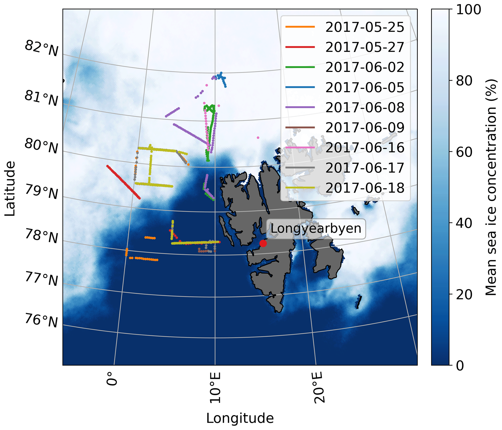
Figure 1 Sections of flight tracks of nine research flights that are included in the analysis after filtering. The mean sea ice concentration during the ACLOUD campaign derived from AMSR2 is shown in the background layer.

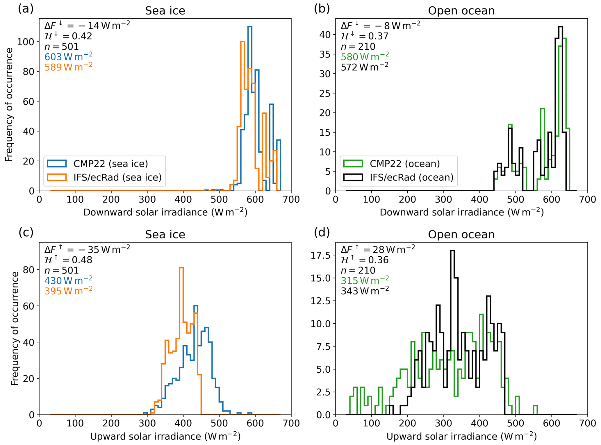
Figure 2 Distribution of (a, b) downward and (c, d) upward solar irradiances for above Polar 5 cloud-free scenes measured by the CMP22 and simulated by ecRad above (a, c) sea ice and (b, d) open ocean. The values in the corner indicate the difference in the mean irradiances between ecRad and CMP22, the corresponding ${\mathcal{H}}^{\uparrow ,\downarrow }$ and the number of included scenes.

Figure 2 shows the frequency distributions of upward and downward solar irradiances measured by the CMP22 pyranometer and simulated by ecRad separately for sea ice and open ocean. The downward irradiances cover the range from 440 to 670 W m⁻². The lower irradiances above open ocean result from the larger solar zenith angles during these flight sections in the morning after takeoff and in the afternoon before landing. There is good agreement between the simulated and observed distribution of downward irradiances with ΔF^↓ = −14 W m⁻² above sea ice (Fig. 2a) and ΔF^↓ = −8 W m⁻² above open ocean (Fig. 2b), which is within the 3 % maximum uncertainty of the CMP22 measurements. The corresponding ℋ^↓ values are calculated with 64 bins of 10 W m⁻² width from 35 to 665 W m⁻² and are 0.42 above sea ice and 0.37 above open ocean.

Observations of upward irradiance above sea ice surfaces range between 300 W m⁻² and mainly 530 W m⁻² (Fig. 2c). The simulations show a similar amount of low irradiances but end abruptly at 450 W m⁻². This upper limit in the IFS seems to be limited to clouds over sea ice. While the distribution of upward irradiances above sea ice is relatively narrow due to the high albedo of the sea ice reducing the cloud radiative effect, the distribution of the upward irradiances above the open ocean with its dark surface and low surface albedo is broader (Fig. 2d). It covers a range of irradiances from 150 to 470 W m⁻² in the simulations and from 30 W m⁻² to mainly 510 W m⁻² in the observations. The low values of the measurements result from a combination of higher solar zenith angles, which are frequently present above open ocean, and scenes without any clouds below Polar 5 where the dark open ocean absorbs the major part of the incoming solar radiation. High values correspond to cloudy scenes reflecting a large amount of the incoming solar irradiance (Fig. 2d). Over ocean, higher upward irradiances are simulated, despite the lower surface albedo. The means above sea ice show a bias of ΔF^↑ = −35 W m⁻² with a ℋ^↑ of 0.48 and above ocean, a bias of ΔF^↑ = 28 W m⁻² with a ℋ^↑ of 0.36.

While the magnitudes of ΔF^↓ are not significant, those of ΔF^↑ exceed the measurement uncertainty and suggest that either the surface or cloud properties are not represented correctly in the IFS.

4 Sensitivity study

There are numerous possible contributors to the observed bias of the reflected solar irradiance. In principle, the radiative transfer and, thus, the reflected solar irradiance is mostly affected by the surface albedo, the cloud fraction and the optical depth of the cloud, neglecting the minor impact of atmospheric gases and aerosols. Following Kokhanovsky (2004), the optical depth τ is related to the cloud properties LWP or LWC, particle effective radius r_eff and density of water ρ_w via

$$\begin{array}{}\text{(3)}& \mathit{\tau }={\displaystyle \frac{\mathrm{3}}{\mathrm{2}}}\cdot {\displaystyle \frac{\mathrm{1}}{{\mathit{\rho }}_{\mathrm{w}}}}\cdot {\displaystyle \frac{\text{LWP}}{r_{\text{eff}}}}={\displaystyle \frac{\mathrm{3}}{\mathrm{2}}}\cdot {\displaystyle \frac{\mathrm{1}}{{\mathit{\rho }}_{\mathrm{w}}}}\cdot {\displaystyle \frac{{\int }_z\text{LWC}\mathrm{d}z}{r_{\text{eff}}}},\end{array}$$

with a vertical integration over the altitude z. However, the optical depth is neither a direct user variable in IFS nor in ecRad. According to the IFS documentation, the mean liquid effective radius r_eff is parameterized following a variation from Martin et al. (1994) by

$$\begin{array}{}\text{(4)}& r_{\text{eff}}={\left({\displaystyle \frac{\mathrm{3}{E}_{\mathrm{d}}(\text{LWC}+\text{RWC})}{\mathrm{4}\mathit{\pi }{\mathit{\rho }}_{\mathrm{w}}k{N}_{\mathrm{d}}}}\right)}^{\frac{\mathrm{1}}{\mathrm{3}}},\end{array}$$

where E_d is an enhancement factor considering an increased dispersion of the droplet size spectrum (Wood, 2000), LWC and RWC are the liquid and rain water content, respectively, k is a factor depending on the relative dispersion of the cloud droplet spectrum set to 0.77 above ocean and N_d is the cloud droplet number concentration. N_d is parameterized via the aerosol number and mass concentrations as a function of prognostic 10 m wind speed accounting for the injection of sea spray aerosols from the ocean (Martin et al., 1994; Boucher and Lohmann, 1995; Lowenthal et al., 2004; Erickson et al., 1986; Genthon, 1992).

These dependencies of the cloud radiative properties and the reflected irradiance finally suggest a sensitivity study testing the contribution of the individual parameters to the observed bias ΔF^↑. For the sensitivity runs, the IFS input to ecRad is adjusted for surface albedo, cloud fraction, LWP, IWP and N_d individually based on observations where possible. The sources of the observed parameters are listed in Table 1 and described in the following Sect. 4.1, 4.2 and 4.3. The reference case is identical to the simulations shown in Sect. 3, where the operational IFS output is fed to ecRad to simulate the solar irradiances.

Table 1 Overview of sets of ecRad simulations performed indicating which parameter was adjusted by which source.

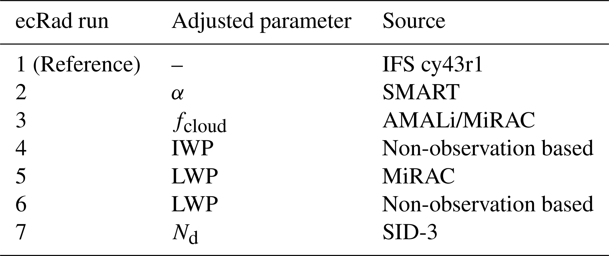
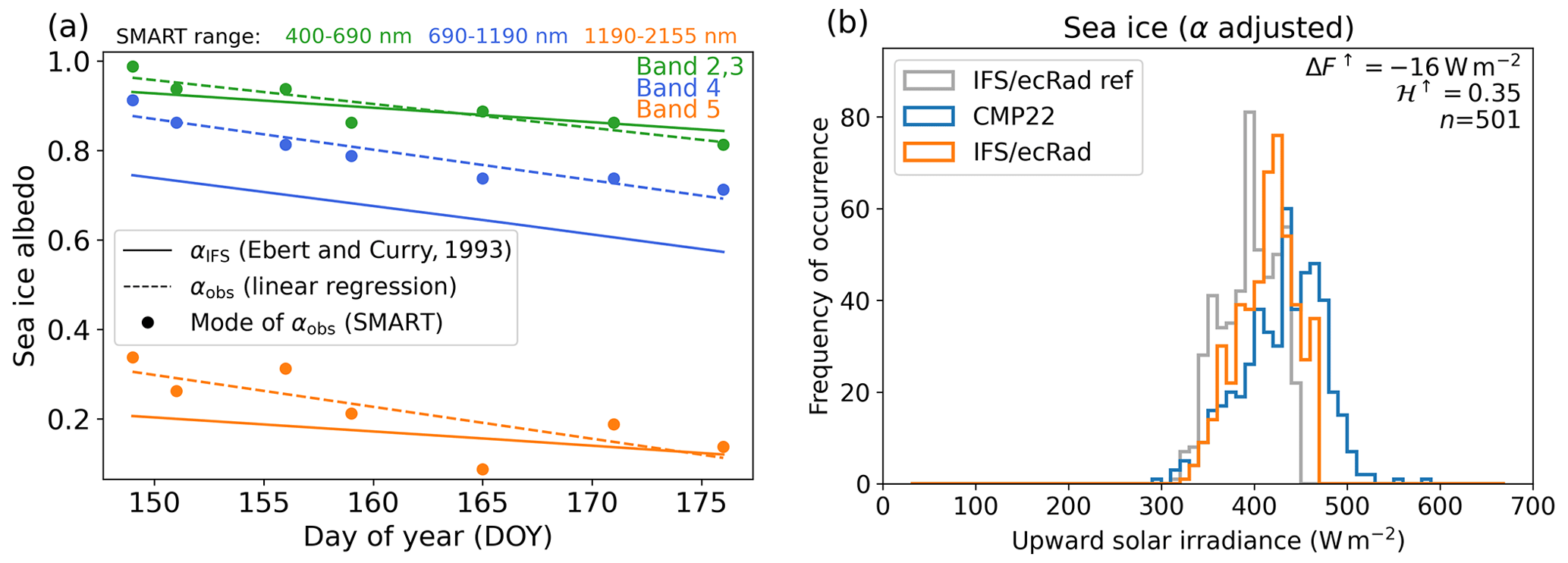
Figure 3 (a) Time series of modes of measured sea ice albedo in the 400–690, 690–1190 and 1190–2155 nm bands (circles) and IFS sea ice albedo climatology (solid lines). The dashed lines show the parameterization for the measurements. (b) Distribution of upward solar irradiances for above Polar 5 cloud-free scenes above sea ice measured by the CMP22 (blue) and simulated by ecRad with the adjusted sea ice albedo (orange) together with the reference simulations (gray).

4.1 Sea ice albedo

In the area covered by the ACLOUD campaign the surface albedo conditions were rather constant above open ocean but more variable above sea ice, which was affected by the melt season. Therefore, this sensitivity run is limited to the observations above sea ice. A realistic constraint of the sea ice albedo is deduced from SMART albedometer measurements from low-level flight sections. Wavelength ranges of 400–690, 690–1190 and 1190–2380 nm are chosen for a wavelength band approach. Figure 3a shows sea ice albedos from measurements of all below-cloud flight sections at flight altitudes below 300 m over sea ice (α_obs, mode values) together with the IFS sea ice albedo climatology in the different bands. The influence of the season is obvious, as the measured sea ice albedo values decrease, mainly because of snow metamorphism to larger grain sizes due to the increase in skin temperature, the accumulating liquid water in the snow layer and the formation of the surface scattering layer (Rosenburg et al., 2023). The IFS sea ice albedo climatology assumes a slower melting season in bands 2, 3 and 5. It underestimates the surface albedo in bands 2 and 3 at the beginning and overestimates it at the end of the campaign, while there is an underestimation in bands 4 and 5 during the whole campaign. These findings support the shortcomings identified by Pohl et al. (2020) with climatologically fixed transitions between the dry snow, melting snow and bare sea ice albedo from Ebert and Curry (1993).

The impact of the faster sea ice albedo reduction and the underestimation of the sea ice albedo on the irradiances is investigated by adjusting the sea ice albedo climatology in a set of ecRad simulations. Linear regressions of the measured sea ice albedo in the three SMART wavelength ranges are used to estimate α_obs on each flight day. The following adjustments are made to the spectral albedo bands in ecRad:

$$\begin{array}{}\text{(5)}& {\displaystyle }\begin{array}{rl}{\mathit{\alpha }}_{\text{IFS,Band}\mathrm{2}/\mathrm{3}}& ={\mathit{\alpha }}_{\text{IFS,250–440}\mathrm{nm}/\text{440–690}\mathrm{nm}}\\ & ={\mathit{\alpha }}_{\text{obs,400–690}\mathrm{nm}}=\mathrm{1.757}-\mathrm{0.005}\cdot \text{DOY}\end{array}\text{(6)}& {\displaystyle }\begin{array}{rl}{\mathit{\alpha }}_{\text{IFS,Band}\mathrm{4}}& ={\mathit{\alpha }}_{\text{IFS,690–1190}\mathrm{nm}}\\ & ={\mathit{\alpha }}_{\text{obs,690–1190}\mathrm{nm}}=\mathrm{1.896}-\mathrm{0.007}\cdot \text{DOY}\end{array}\text{(7)}& {\displaystyle }\begin{array}{rl}{\mathit{\alpha }}_{\text{IFS,Band}\mathrm{5}}& ={\mathit{\alpha }}_{\text{IFS,1190–2380}\mathrm{nm}}\\ & ={\mathit{\alpha }}_{\text{obs,1190–2155}\mathrm{nm}}=\mathrm{1.367}-\mathrm{0.007}\cdot \text{DOY},\end{array}\end{array}$$

where DOY is the day of the year. Bands 2 and 3 are considered together due to the sparse SMART coverage of band 2; bands 1 and 6 are kept unchanged as they lie out of the SMART wavelength range.

Table 2 ΔF^↑ of the mean simulated and observed upward solar irradiance distributions of ecRad simulations and CMP22 observations and their corresponding ℋ^↑ for all sets of simulations.

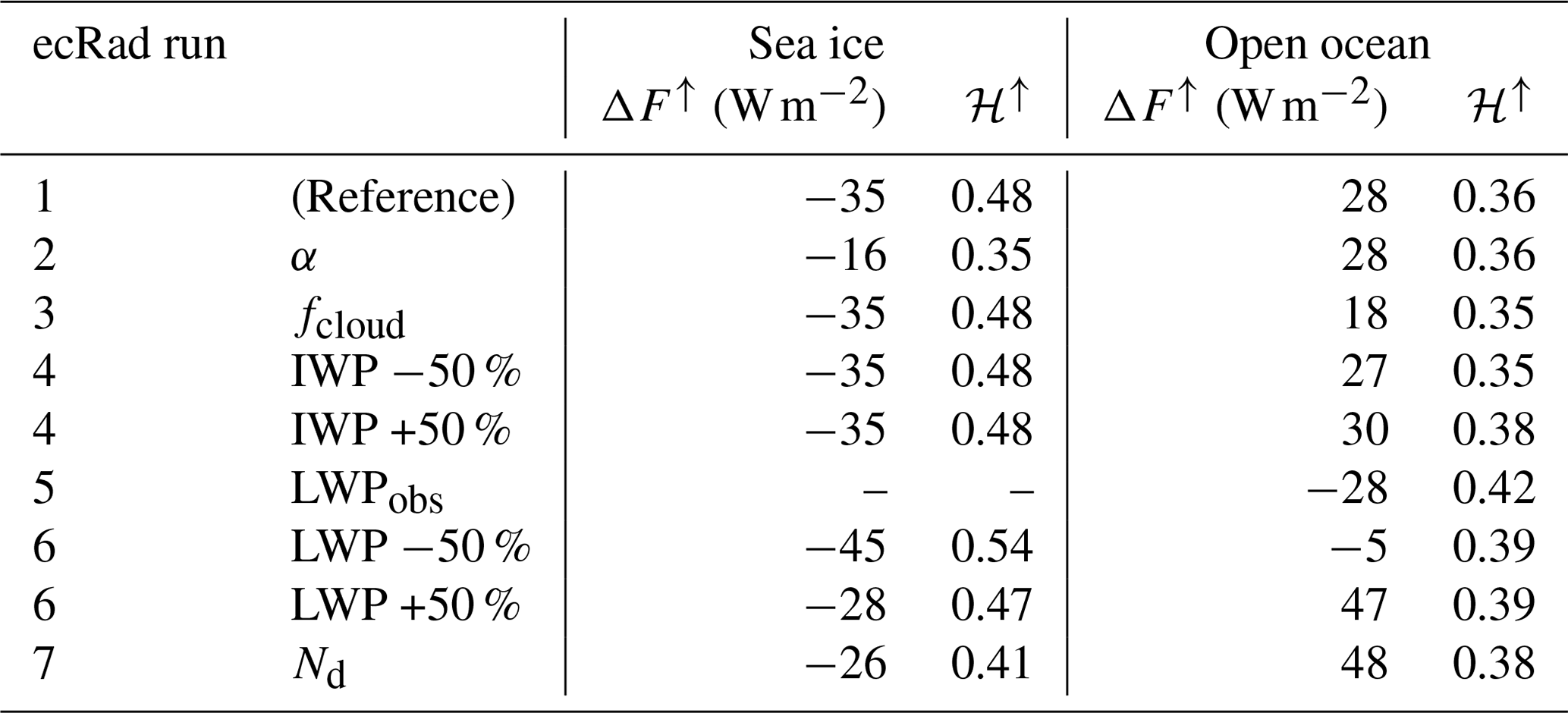
The results of the modified ecRad run are shown in Fig. 3b and compared with the reference run and the observations. Due to the higher sea ice albedo, especially for band 4, the sensitivity run on average results in higher upward solar irradiances. In comparison with the reference distribution, the adjusted distribution emerges with 320 W m⁻² at a 10 W m⁻² higher upward irradiance, but ends with 20 W m⁻² higher at 470 W m⁻². The distribution itself is shifted to higher values throughout all upward irradiances with the highest peak located between 420 and 430 W m⁻². The bias ΔF^↑ decreases accordingly from −35 to −16 W m⁻². The corresponding ℋ^↑ decreases from 0.48 to 0.35. These and all the following values from the subsequent ecRad runs are summarized in Table 2. Thus, the replacement of the original sea ice albedo reduces the gap between the simulated and the observed irradiances by more than 50 %. This indicates that the representation of the sea ice albedo in the IFS causes one major part of the disagreement. Another major part may be caused by the representation of clouds.

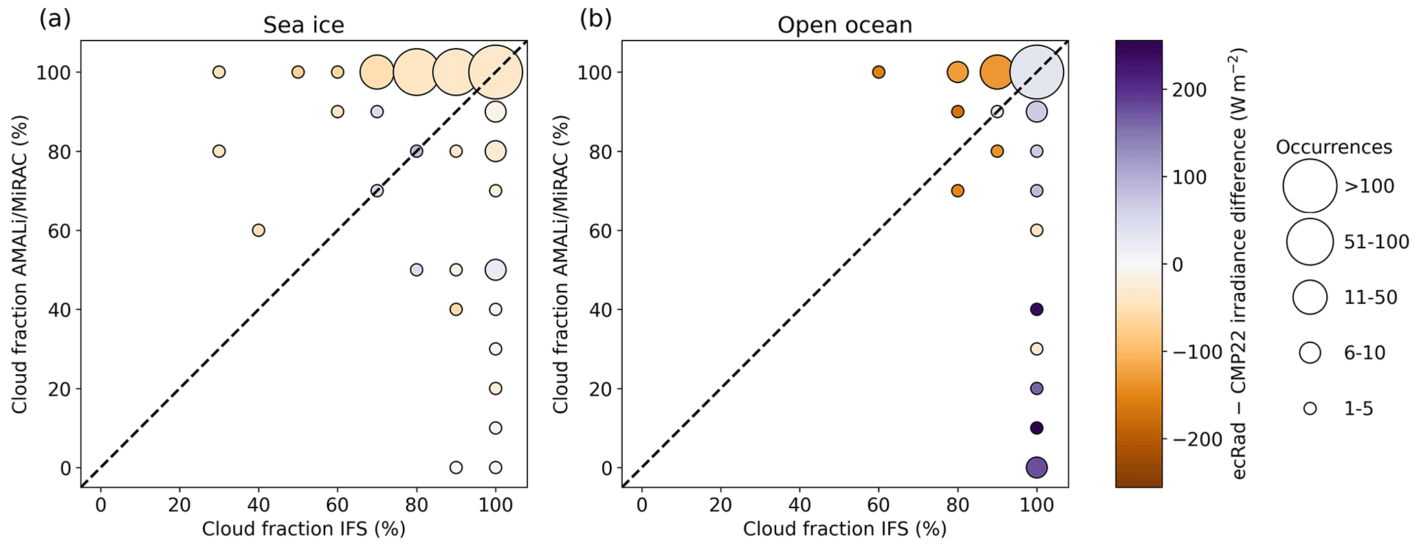
Figure 4 Two-dimensional frequency distributions of IFS cloud fractions and observational cloud fractions based on AMALi and MiRAC above (a) sea ice and (b) open ocean, with the upward irradiance differences between ecRad simulations and CMP22 observations shown as colored circles.

4.2 Cloud fraction

The cloud fraction of the IFS is compared with airborne remote sensing observations. A lidar-based cloud mask from the AMALi cloud top altitude product (Kulla et al., 2021) is used in combination with a radar-based cloud identification from MiRAC. Merging both types of cloud identification leads to a remote-sensing-based cloud fraction f_cloud, RS that accounts for the different sensitivities of radar and lidar. This cloud fraction is calculated from 60 s flight sections. As these flight sections cover only a cross section of a grid box, there is an imbalance between the observed variability of the cloud fraction and the grid box mean. Especially low cloud fractions are less likely in IFS. Sections above sea ice and open ocean are shown separately in Fig. 4, which compares the combinations of observed and forecasted cloud fractions together with the corresponding mean upward irradiance differences between ecRad simulations and observations. An ideal representation of the observed clouds in the IFS would entail all data circles to lie on the dashed diagonal line with white indicating no bias in the observed and simulated solar irradiances. However, especially above open ocean, the remote sensing cloud fraction covers the whole range from cloudless to overcast conditions, while the IFS shows only little variability, with cloud fractions ranging between 60 % and 100 %. The data below the dashed diagonal correspond to an overestimation of the cloud fraction by the IFS, which causes the positive irradiance differences to dominate. In theory, the data above the 1:1 line in Fig. 4b correspond to an underestimation of the cloud fraction by the IFS, in association with negative irradiance differences indicated by orange shades, and vice versa. Data that do not follow this theory are most likely caused by the possible imbalance of cloud fractions induced by comparing the entire grid box with the aircraft transect. Data points where the cloud fractions agree are mostly observed for overcast conditions. In this case, the bias of the ecRad simulations is negative above sea ice and positive above open ocean.

A set of ecRad simulations is performed where the prognostic cloud fraction f_{cloud, IFS, level} is replaced by the observations taking into account the vertical distribution of the clouds. As a basic approach, the IFS cloud profiles are kept constant. To account for maximum overlap, this approach ensures that the maximum cloud fraction profile is replaced by the remote sensing cloud fraction. All other levels are scaled accordingly, adopting the original shape of the cloud fraction profile. This is realized by replacing f_{cloud, IFS, level} with $f_{\text{cloud,\hspace{0.17em}level}}^{\prime }$ calculated via

$$\begin{array}{}\text{(8)}& f_{\text{cloud,\hspace{0.17em}level}}^{\prime }=f_{\text{cloud,\hspace{0.17em}RS}}\cdot {\displaystyle \frac{f_{\text{cloud,\hspace{0.17em}IFS,\hspace{0.17em}level}}}{f_{\text{cloud,\hspace{0.17em}IFS,\hspace{0.17em}max}}}},\end{array}$$

where f_{cloud, IFS, max} is the maximum cloud fraction of all 137 model levels.

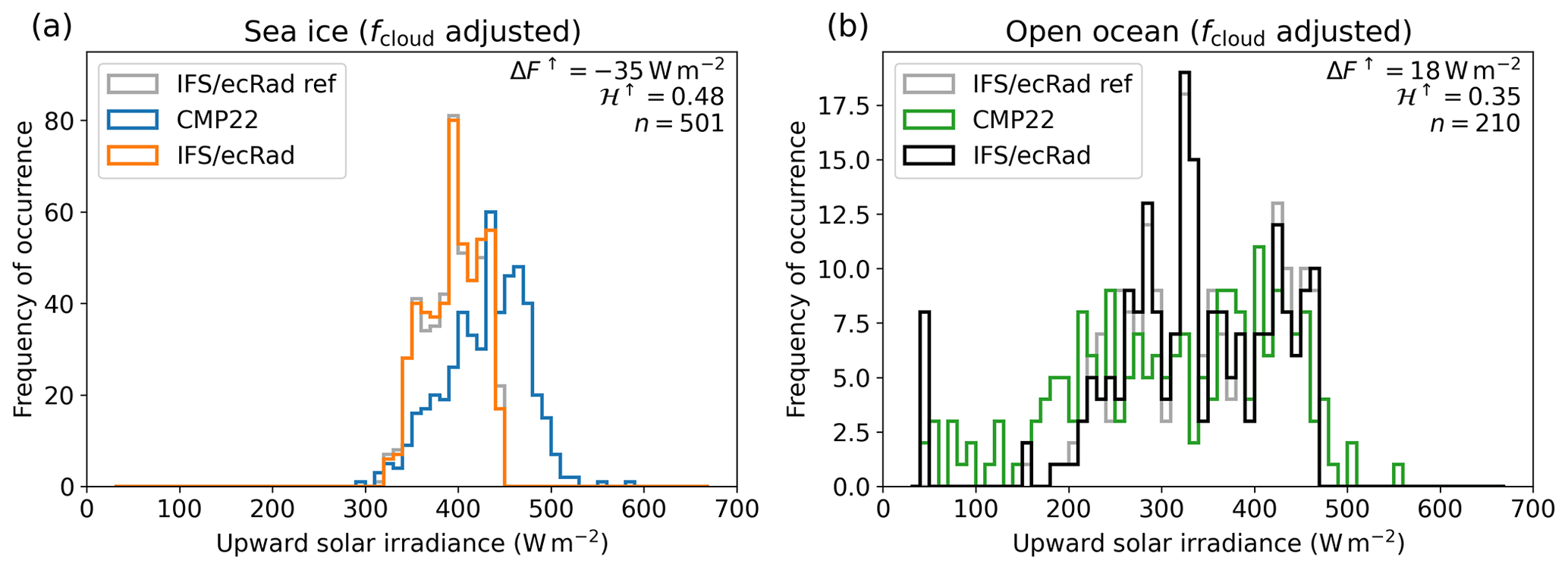
Figure 5 Distribution of upward solar irradiances above (a) sea ice measured by the CMP22 (blue) and simulated by ecRad with the adjusted cloud fractions (orange) together with the reference simulations (gray), and above (b) open ocean measured by the CMP22 (green) and simulated by ecRad with the adjusted cloud fractions (black) together with the reference simulations (gray).

Figure 5 compares the irradiance distributions from the ecRad simulations with the replaced cloud fraction against the reference run and the observations. Above sea ice, the simulated irradiance distribution does not change significantly. Due to the high surface albedo, small changes in f_cloud do not significantly reduce the reflected radiation. Thus, ΔF^↑ remains at −35 W m⁻² with ℋ^↑ remaining at 0.48. Above open ocean, occurrences of upward solar irradiance between 200 and 460 W m⁻² are mainly lower compared to the reference distribution. This reduction enables a new mode to occur between 40 and 50 W m⁻², and thus the replacement by the observed cloud fraction results in a higher number of data with low reflected irradiances. This results from the overestimation of prognostic f_cloud, which may be linked to broken cloud conditions that cannot be resolved by the IFS. ΔF^↑ is reduced by 36 % from 28 to 18 W m⁻² with a corresponding ℋ^↑ decrease from 0.36 to 0.35 (see Table 2).

4.3 Macro- and microphysical cloud properties

4.3.1 Ice water path

The low-level clouds observed during ACLOUD are mostly of mixed-phase character although dominated by liquid droplets (Ruiz-Donoso et al., 2020; Klingebiel et al., 2023). No direct observations are available from ACLOUD to test the relevance of the representation of ice crystals in the IFS to the cloud-reflected solar irradiance. Therefore, the prognostic IWP in terms of the specific cloud IWC is both increased and reduced on a theoretical basis by 50 % in two sets of simulations. This increase (reduction) in IWP is propagated to an increase (reduction) in the ice effective radius according to Sun and Rikus (1999) and Sun (2001). Over sea ice, the simulated upward irradiance did not change. Above open ocean, the mean simulated irradiance is only increased by 1 W m⁻² when the IWP is increased by 50 % and is only reduced by 2 W m⁻² when the IWP is reduced by 50 %. Thus, more cloud ice increases the bias of the irradiance simulations and less cloud ice reduces the bias. These small effects confirm the relatively low IWP during ACLOUD reported by Klingebiel et al. (2023) and indicate that the cloud droplets dominate the cloud radiative properties. Here, ice crystals may not directly cause the bias between simulated and observed irradiances. Similarly, ice crystal shape and size will not significantly impact the irradiance reflected by these liquid-dominated clouds (Ehrlich et al., 2008). Also the choice of the ice optics parameterization within ecRad can impact the reflected irradiance (as shown by, e.g., Wolf et al., 2020). However, a model–observations comparison in this regard would require an agreement between the IWC in the IFS and the observations. This agreement cannot be verified with the Polar 5 instrumentation.

4.3.2 Liquid water path

To adjust the prognostic LWP in the IFS with observations, LWP measurements derived from passive microwave remote sensing observations on Polar 5 are applied. However, the LWP product by the passive 89 GHz channel from MiRAC (Kliesch and Mech, 2021) is only available above open ocean. Above sea ice with its high emissivity the retrieval sensitivity is not sufficient, which is why this sensitivity study is firstly limited to open ocean. To confront the observed LWP above open ocean with the IFS output, the prognostic liquid cloud mass mixing ratio is converted to LWC and vertically integrated between the surface and Polar 5 flight altitude to the IFS LWP.

The combinations of the observed and the prognostic LWP are shown for the 210 scenes in Fig. 6. Observations are again 60 s averages of LWP including cloud-free data and IFS values are the grid box mean all-sky LWP. They reveal the tendency of the IFS to predict a too-high LWP, while the observations rarely show an LWP above 150 g m⁻². This point-by-point mismatch indicates that cloud heterogeneity is high for the observed clouds. This is typical for low-level clouds over open ocean (Schäfer et al., 2018), especially when linked to cold air outbreaks. Similar to the discussion in Sect. 4.2, this mismatch partly results from the imbalance of Polar 5 sampling along a straight flight leg and the IFS providing grid box means. The exact position of the horizontal cloud structures cannot be forecasted precisely and also may change within the time offset between observations and IFS output. However, as shown in Fig. 6, the differences in irradiance correlate with the mismatch in LWP. Even within a single research flight, both overestimations and underestimations of the observed LWP by a factor of 2 occur.

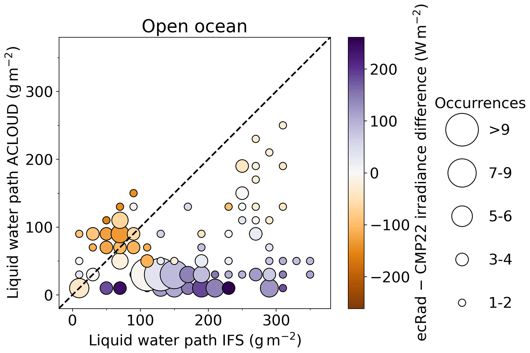
Figure 6 Combinations of prognostic IFS LWP and observed LWP based on MiRAC with classes of absolute frequency represented by circle size and upward solar irradiance differences between ecRad simulations and CMP22 observations represented by colors.

A set of ecRad simulations is performed with adjusted LWP. The specific cloud LWC q_liq in ecRad is replaced with

$$\begin{array}{}\text{(9)}& q_{\text{liq}}^{\prime }=q_{\text{liq}}\cdot {\displaystyle \frac{{\text{LWP}}_{\text{obs}}}{{\text{LWP}}_{\text{IFS}}}},\end{array}$$

where LWP_obs is the ACLOUD LWP and LWP_IFS is the prognostic integrated LWP, so that the LWC profile shape is kept. The liquid effective radius is recalculated, respectively, considering the changed LWC in Eq. (4). After adjusting, r_eff is limited to 4–30 µm to match the IFS constraints again. N_d remains fixed.

The distributions of the upward solar irradiance for the observations, the reference simulations and the adjusted simulations with replaced LWP and r_eff are shown in Fig. 7. Compared to the reference distribution, the adjusted distribution emerges already at 80 W m⁻² instead of 150 W m⁻² and ends at upward irradiances 20 W m⁻² lower than before. The main mode ranges between 230 and 290 W m⁻² instead of between 320 and 340 W m⁻². Adjusting the LWP based on observations leads to a change in the correct direction by reducing the upward solar irradiances. Compared to the observations, this impact is too strong resulting in a conversion of the overestimation to an underestimation. The adjustment overcompensates the reference bias between the simulated and the observed distribution of upward irradiances with ΔF^↑ = −28 W m⁻², and the corresponding ℋ^↑ increase is included in Table 2.

To quantify the impact of LWP uncertainties not only for clouds above open ocean but also above sea ice, the prognostic LWP is both increased and reduced artificially by 50 % in two sets of simulations, with r_eff changing accordingly. N_d remains fixed. ΔF^↑ changes above sea ice from −35 to −45 W m⁻² by the reduction in the LWP, and to −28 W m⁻² by the increase in the LWP. This qualitatively matches the findings from Solomon et al. (2023) that IFS produces too-small LWPs in the central Arctic. The bias ΔF^↑ above open ocean changes from 28 W m⁻² in the reference case to −5 W m⁻² by reducing the LWP and to 47 W m⁻² by doubling the LWP. This indicates that the adjustments of the IFS need to be different above sea ice compared to open ocean in order to match the observations during the ACLOUD campaign. Above sea ice, the increase in the LWP and the implicit change in r_eff improve ΔF^↑ (Fig. 8a) by a slightly higher emergence of the upward irradiance distribution at 320 W m⁻², by slightly higher irradiances over a wide range of the distribution and by keeping the same end of the distribution as in the reference case. Above open ocean, the decrease in the LWP and the implied r_eff improve ΔF^↑ (Fig. 8b) by shifting the entire distribution to 20–30 W m⁻² lower upward irradiances. Possible reasons for the different LWP change directions may lie in differences in cloud physics between sea ice and open ocean. Above open ocean, especially during cold air outbreaks, turbulent surface fluxes of sensible and latent heat are magnitudes larger than above sea ice (e.g., Hartmann et al., 1997), and cloud droplet number concentrations are known to differ (Young et al., 2016). The changes shown by the sensitivity study match qualitatively the findings of Moser et al. (2023) with higher N_d above sea ice than above open ocean, assuming a linear relation between LWC and N_d as found by Leaitch et al. (2016) and Dionne et al. (2020). Although the bias ΔF^↑ above open ocean is largely reduced, ℋ^↑ is increased to 0.39 due to significant changes in the shape of the irradiance distribution, especially at the upper end where the sharp cut-off of the highest irradiances is reduced from 470 to 440 W m⁻² because of the lower LWP.

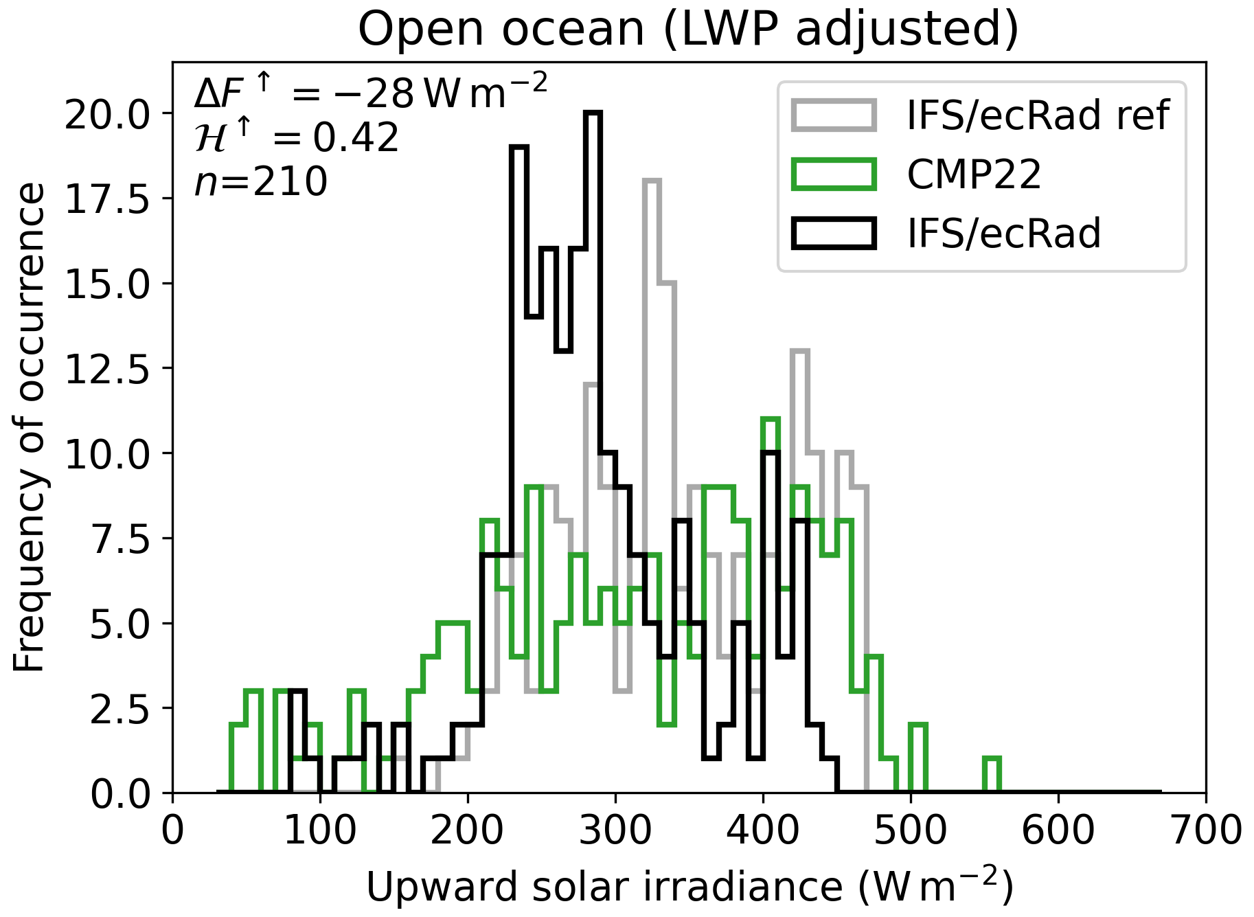
Figure 7 Distribution of upward solar irradiances above open ocean measured by CMP22 (green) and simulated by ecRad (black) with the adjusted LWP and liquid effective radius based on the MiRAC LWP scaling of the prognostic LWP together with the reference simulations (gray).

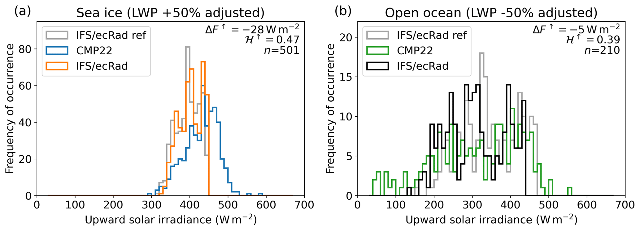
Figure 8 Distribution of upward solar irradiances measured by CMP22 (blue) and simulated by ecRad (a) above sea ice with a 50 % increased LWP and (b) above open ocean with a 50 % decreased LWP, with subsequent adjustments to the liquid effective radius (orange) together with the reference simulations (gray).

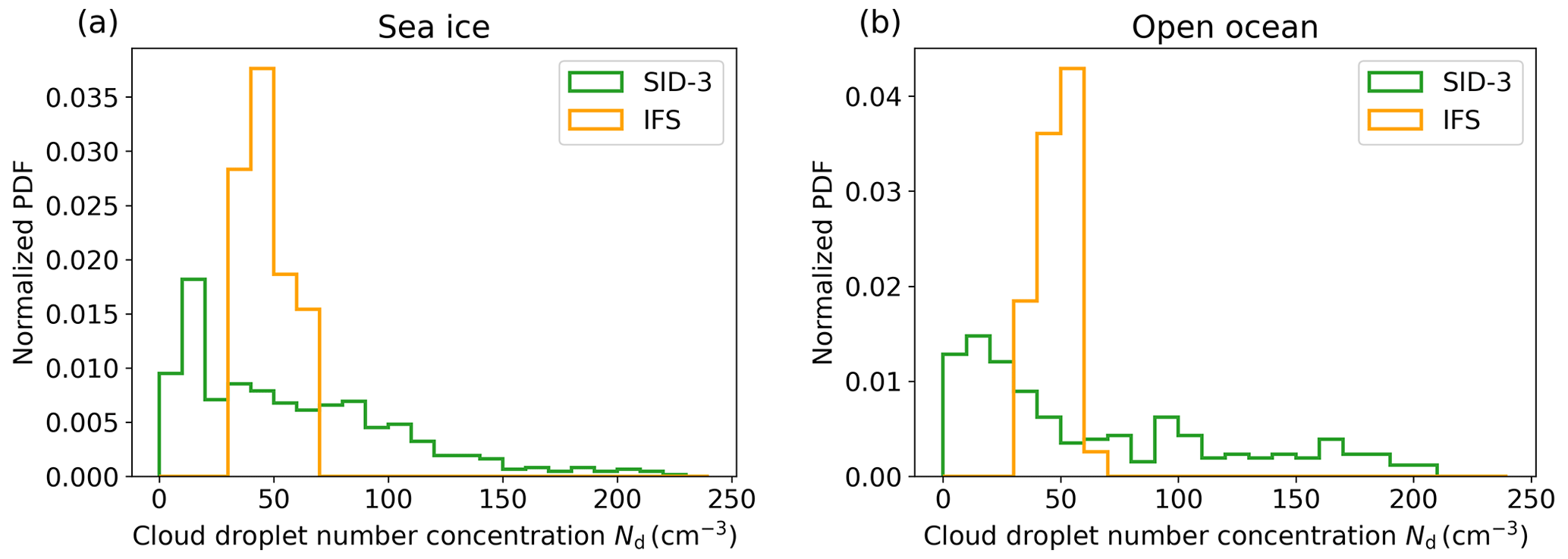
Figure 9 Distributions of cloud droplet number concentrations measured by the SID-3 and parameterized within IFS above (a) sea ice and (b) open ocean averaged over 60 s intervals.

4.3.3 Cloud droplet number concentration

The cloud droplet number concentration affects the cloud radiative properties by occurring in Eq. (4). The parameterized N_d in the IFS is compared with in situ observations available from the SID-3 cloud probe aboard Polar 6 (Schnaiter and Järvinen, 2019). However, the flight track of Polar 5 does not always match the path of Polar 6. Nevertheless, on a statistical basis, Polar 5 and Polar 6 sampled the same cloud and air mass regimes. Figure 9 shows the result of the N_d parameterization described at the beginning of Sect. 4 together with the in situ observations averaged over 60 s intervals for the filtered scenes. The number concentrations in the IFS are within a narrow range between 36 and 69 cm⁻³, with slightly higher concentrations above sea ice due to slightly higher prognostic wind speeds leading to a stronger injection of sea spray aerosols to the atmosphere, which can act as cloud condensation nuclei. The in situ observations show a much broader range up to 230 cm⁻³. The observed low values of N_d mostly result from cloud edges or cloud-free flight sections and are not comparable to the mean grid box values of the IFS. However, the high N_d values of over 200 cm⁻³ measured by SID-3 are not captured by the IFS. The findings from Moser et al. (2023) for two different aircraft campaigns in the Arctic with higher N_d above sea ice compared to open ocean are different from the ACLOUD observations, which may be attributed to a different season and different dominating air masses.

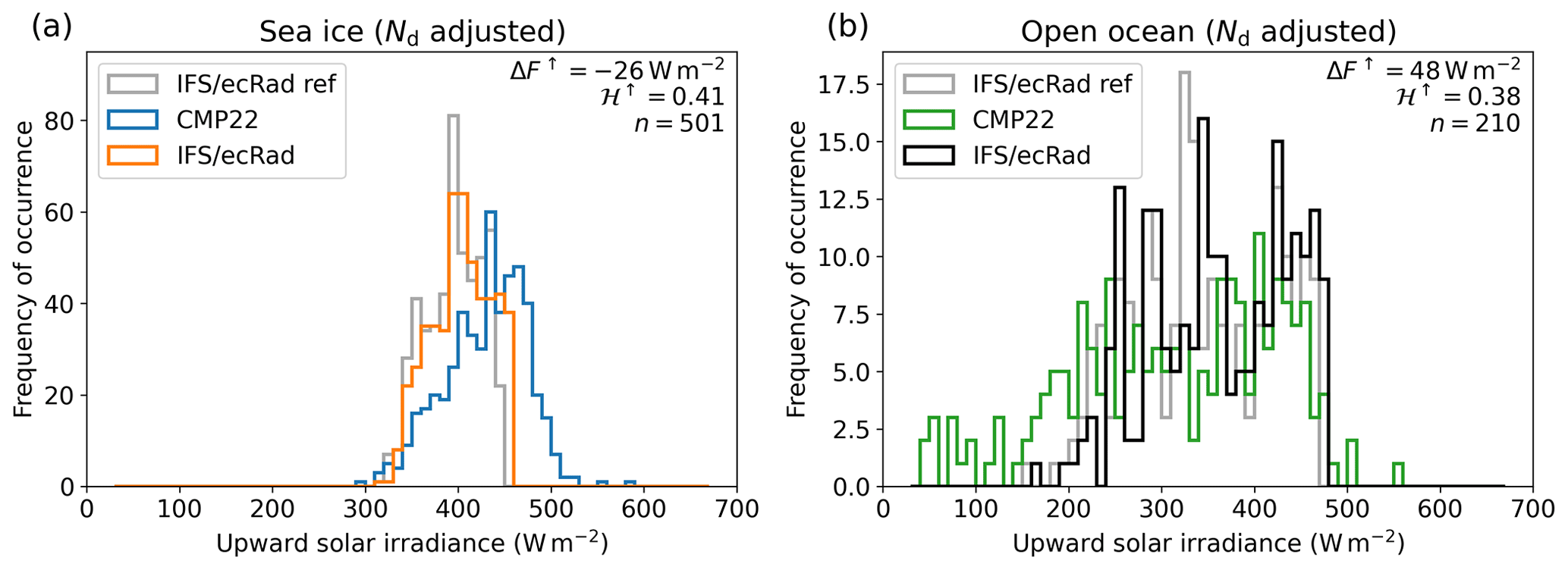
Figure 10 Distribution of upward solar irradiances above (a) sea ice measured by the CMP22 (blue) and simulated by ecRad with the adjusted number concentration and liquid effective radius (orange) together with the reference simulations (gray), and above (b) open ocean measured by the CMP22 (green) and simulated by ecRad with the adjusted number concentrations and liquid effective radius (black) together with the reference simulations (gray).

To investigate the impact of more realistic cloud droplet number concentrations on the reflected solar irradiance, a new set of ecRad simulations is performed with adjusted N_d. The lower boundary N_{d, obs, min} is fixed to N_{d, IFS, min} = 36 cm⁻³ to account for the IFS grid box size, which cannot resolve cloud edges with only a few cloud droplets. The upper boundary N_{d, obs, max} is set to 200 cm⁻³, excluding only the highest values of the distribution's tail. The initial N_d, IFS appearing as cloud droplet number concentration in Eq. (4) is replaced by

$$\begin{array}{}\text{(10)}& \begin{array}{rl}{N}_{\text{d,\hspace{0.17em}IFS}}^{\prime }=& (N_{\text{d,\hspace{0.17em}IFS}}-N_{\text{d,\hspace{0.17em}IFS,\hspace{0.17em}min}})\\ & \cdot {\displaystyle \frac{N_{\text{d,\hspace{0.17em}obs,\hspace{0.17em}max}}-N_{\text{d,\hspace{0.17em}obs,\hspace{0.17em}min}}}{N_{\text{d,\hspace{0.17em}IFS,\hspace{0.17em}max}}-N_{\text{d,\hspace{0.17em}IFS,\hspace{0.17em}min}}}}+N_{\text{d,\hspace{0.17em}obs,\hspace{0.17em}min}},\end{array}\end{array}$$

where $N_{\text{d,\hspace{0.17em}IFS}}^{\prime }$ is the adjusted cloud droplet number concentration. N_{d, IFS, min} (N_{d, IFS, max}) is the minimum (maximum) cloud droplet number concentration from the IFS parameterization and N_{d, obs, min} (N_{d, obs, max}) is the minimum (maximum) cloud droplet number concentrations derived from in situ observations. The liquid effective radius is recalculated, respectively, considering the changed N_d in Eq. (4), while LWC remains fixed. Figure 10 shows the result of these adjustments. In general, the increase in N_d increases the reflected solar irradiance. Above sea ice, the maximum values of upward solar irradiance reach 460 W m⁻² instead of 450 W m⁻² while the minimum remains unchanged. In between, the distribution is shifted to slightly higher irradiances. Above open ocean, the entire distribution of adjusted upward solar irradiances is shifted to higher irradiances, with the minimum and maximum ranging 10 W m⁻² higher. ΔF^↑ decreases by scaling N_d above sea ice to −27 W m⁻², but increases above open ocean to 48 W m⁻². ℋ^↑ changes to 0.41 above sea ice and to 0.38 above open ocean accordingly. Above sea ice, the N_d parameterization may be optimized by a higher variability. Above open ocean, this larger variability of N_d increases the overestimation by ecRad. The observed differences in N_d between sea ice and open ocean surface are a minor issue, and they are not taken into account by the parameterization in IFS, but can occur by different sea salt aerosol production mechanisms above sea ice (blowing snow) and open ocean (wave breaking), as described by, e.g., Confer et al. (2023).

5 Conclusions

Airborne observations of broadband solar irradiance measured above Arctic low-level clouds during the ACLOUD airborne campaign in May/June 2017 were used to evaluate the corresponding solar irradiances simulated by the IFS of the ECMWF. For this purpose, the ecRad radiative transfer scheme embedded in IFS was run in an offline mode using the output of the corresponding IFS 00:00 UTC runs as input. While there is agreement within the observational uncertainty between the measured and simulated downward solar irradiance, larger differences exceeding the pyranometer's uncertainty are found for the upward solar irradiance. In a sensitivity study constrained by surface and cloud properties observed during ACLOUD, this bias was attributed to issues of the IFS in representing sea ice albedo and low-level, liquid-dominated mixed-phase clouds. The impacts of different surface and cloud properties were quantified. The limitations of the sea ice model by Ebert and Curry (1993) to represent the change of sea ice albedo during the melting season cause more than 50 % of the observed bias. A comparison with airborne observations reveals an underestimation of the sea ice albedo by the IFS, especially in the wavelength band from 690 to 1190 nm. Implementing the measured sea ice albedo values into ecRad decreases the bias between the simulations and the observations to −16 W m⁻².

A misrepresentation of cloud fraction is assessed by active cloud remote sensing. The observed cloud fraction does not change ΔF^↑ above sea ice, but reduces the bias from 28 to 18 W m⁻² above open ocean where the observations show lower cloud fractions and the difference between the dark ocean and clouds is particularly large. The impact of cloud ice was quantified by artificially changing the IWP of the IFS output. The sensitivity of the upward solar irradiance to variations in the IWP of the underlying clouds is nearly negligible with the largest impact of −2 W m⁻² above open ocean by reducing the IWP by 50 %. The cloud optical properties strongly depend on the LWP of the clouds. Confronting the prognostic LWP with airborne observations (above open ocean only) reduces the positive ΔF^↑ strongly and overcompensates it with a bias of −28 W m⁻². To estimate the effect of a misrepresentation of LWP also above sea ice, a non-observation-based sensitivity study was performed. By increasing the LWP by 50 %, ΔF^↑ improves above sea ice to −28 W m⁻², and by decreasing the LWP by 50 %, ΔF^↑ improves to −5 W m⁻².

Airborne in situ observations have shown that the range of N_d in the IFS is significantly smaller than measured. This affects the cloud radiative properties simulated by the IFS. Adjusting N_d, which occurs in the parameterization of the liquid effective radius from Martin et al. (1994) within a range of 36–69 cm⁻³, to a broader range of number concentrations found in the observations (36–200 cm⁻³) results in a bias reduction above sea ice to −27 W m⁻² and in a bias increase to 48 W m⁻² above open ocean.

The sensitivity study identifies the misrepresentation of the surface albedo as the largest contributor to the bias above sea ice. The sea ice albedo values in the IFS are applied as representative constant albedo values of dry snow, melting snow and bare sea ice for fixed times of the year. Replacing these with a sea ice albedo parameterization that considers mixtures of different sea ice types and their specific albedos depending on parameters such as the surface temperature may improve the ability of the IFS in correctly simulating the upward solar irradiances in the Arctic (Jäkel et al., 2019b, 2023). The uncertainties of cloud radiative effects in the IFS significantly depend on the surface type below the clouds. With large contributions to the bias improvement given by realistic cloud droplet number concentrations and LWPs above sea ice and by realistic cloud fractions and LWPs above open ocean, a large amount of the bias could be attributed to the representation of cloud micro- and macrophysical properties during the ACLOUD campaign.