LIME: Lunar Irradiance Model of ESA, a new tool for absolute radiometric calibration using the Moon

Absolute calibration of Earth observation (EO) sensors is key to ensuring long-term stability and interoperability, and it is essential for long-term global climate records and forecasts. The Moon provides a photometrically stable calibration source within the range of the Earth's radiometric levels and is free from atmospheric interference. However, to use this ideal calibration source, one must model the variation in its disc-integrated irradiance resulting from changes in Sun–Earth–Moon geometries. The Lunar Irradiance Model of the European Space Agency (LIME) is a new lunar irradiance model developed from ground-based observations acquired using a lunar radiometer operating from the Izaña Atmospheric Observatory near Mount Teide, located in Tenerife, Spain. Nightly top-of-atmosphere (TOA) irradiance is determined using the Langley plot method, and each observation is traceable to the international system of units (SI) through the radiometer calibration performed at the National Physical Laboratory (NPL). Approximately 590 lunar observations acquired between March 2018 and December 2022 currently contribute to the model parameter derivation, which builds on the widely used ROLO (Robotic Lunar Observatory) model analytical formulation. This paper presents the strategy used to derive LIME parameters: the characterisation of the lunar radiometer, the derivation of nightly top-of-atmosphere lunar irradiance and a description of the model parameter derivation, along with the associated metrologically rigorous uncertainty. The model output has been compared to PROBA-V, Pléiades and Sentinel-3B, as well as to the VITO implementation of the ROLO model. Initial results indicate that LIME predicts 3 %–5 % higher lunar-disc-integrated irradiance than the ROLO model for the visible and near-infrared channels. The model output has an expanded (k=2) radiometric uncertainty of ∼ 2 % at the lunar radiometer wavelengths, and it is expected that planned observations until at least 2024 further constrain the model parameters in subsequent updates.

1 Introduction

Earth observation satellites provide essential data sets for a wide range of commercial, societal and scientific applications. At present, long-term sustained operational Earth observation programmes, such as the Copernicus Sentinels, offer reliable environmental information services to diverse users. The data acquired through these programmes provide a unique opportunity to understand the changing dynamics of our planet, which has the potential to significantly influence socio-political decisions. However, for long-term environmental and climate records, the stability and interoperability of Earth observation sensors are key.

These sensors are rigorously characterised pre-flight in laboratories; however, the harsh environment of space and the harshness of launch can lead to ground-to-orbit and in-orbit degradation, meaning that in-flight calibration is essential to ensure satellite accuracy, stability and interoperability. In addition to onboard calibration systems, which are also susceptible to degradation in space, vicarious calibration methods are often used, including the use of instrumented field sites (e.g. the automated sites of RadCalNet (Bouvet et al., 2019) and one-off measurements of ground field campaigns (Thome et al., 1993; Thome, 2001)), the use of pseudo-invariant calibration sites (PICS) (Cosnefroy et al., 1996; Lacherade et al., 2013a; Bouvet, 2014), and the use of natural phenomena, e.g. Rayleigh scattering, deep convective clouds and sun glint (Sterckx et al., 2013; Alhammoud et al., 2018).

One important vicarious reference source is the Moon. With no atmosphere, the surface of the Moon is extremely stable long term (Kieffer, 1997). Geostationary satellite instruments sometimes observe the Moon in the “dark space corners” of their field of view, and low-Earth-orbit sensors can be manoeuvred to observe the Moon. Many satellites already use the Moon as a calibration source, particularly to monitor long-term radiometric stability. The Moon is also used to monitor atmospheric aerosols in a diurnal cycle (Barreto et al., 2019), where lunar photometry has emerged as a suitable approach to extend aerosol remote sensing capabilities during nocturnal period, which is critical for climate studies, especially for high-latitude and polar regions (Barreto et al., 2013, 2017; Berkoff et al., 2011; González et al., 2020; Román et al., 2020).

However, to use the Moon as a radiometric reference, it is necessary to model the lunar disc irradiance variations resulting from the changing lunar phase angle and lunar libration. There are many periodic cycles that apply to the Moon, Earth and Sun geometry. The cycle with the longest period is called the Saros cycle, and its duration is 223 synodic months, which is 18 years, 11 d and 8 h. After this cycle, the Earth, Moon and Sun return to the same relative geometry. The shortest cycle is the variation in phase angle which takes about 28 d between two full-moon events.

Previous models of lunar irradiance, most notably the Robotic Lunar Observatory (ROLO) model (Kieffer and Stone, 2005), have proven to be valuable tools for the monitoring of radiometric stability. However, ROLO has an expected uncertainty of 5 %–10 % (Stone and Kieffer, 2004) and is not currently used as a reference for absolute radiometric calibration. The lunar photometry and calibration community are actively working to improve the uncertainties in the ROLO model (Smith et al., 2012; Stone et al., 2020, among others), mostly based on empirical corrections derived from observations at high altitude in pristine conditions, such as the NASA Airborne Lunar Spectral Irradiance (air-LUSI) project (Grantham et al., 2022) or those performed by Barreto et al. (2017) and Román et al. (2020).

This paper outlines the strategy used to develop a lunar irradiance model from new ground-based measurements obtained from a high-altitude location. Section 2 provides a summary of lunar calibration and of ROLO, on which the Lunar Irradiance Model of the European Space Agency (LIME) is based. Section 3 describes the methodology for the lunar observations and derivation of LIME. Section 4 describes the calibration of the instrument used for the lunar observations, essential for providing the SI traceability and minimising the uncertainty in the resulting model. The results of the current implementation of the model are presented along with an initial comparison to several data sets. This new model is envisaged to be used as a reliable vicarious reference for absolute radiometric calibration, not only for Earth observation (EO) sensors but also for at-ground photometry for night aerosol retrieval. Model reliability has been ensured by means of a metrologically rigorous uncertainty analysis in addition to a comprehensive validation with satellite sensors.

2 Lunar calibration background

2.1 The Moon as a tool for post-launch calibration

Absolute radiometric calibration of space-borne optical instruments using ground-based measurements of terrestrial ground targets is challenging as it requires accounting for the interaction of sunlight with the atmosphere. These difficulties can be partially mitigated by acquiring measurements taken from aircraft, high above the bulk of the optically significant part of the atmosphere. Both ground-based and airborne methods can be labour-intensive, costly and reliant on favourable weather conditions.

For radiometric intercalibration based on comparison at the top-of-atmosphere (TOA) reflectance level of terrestrial calibration targets, the variability of the atmosphere and environmental surface processes is also an issue. These variations create difficulties in cross-calibrating instruments and ensuring continuity, especially in cases where there are gaps between instrument lifetimes.

These problems are partially addressed by the careful selection of “pseudo-invariant calibration sites” (PICS), typically located in deserts. Initiatives like RadCalNet (Bouvet et al., 2019) further contribute to overcoming these challenges by providing continuous automated in situ measurements of both surface and atmospheric conditions.

Observations indicate that the Moon is largely photometrically stable, with estimates of the change in reflectance on the order of 10⁻⁸ yr⁻¹, based on the rate of meteoric impacts and the Moon's geological age (Kieffer, 1997). Additionally, the Moon exhibits a similar reflectance (approximately 10 % throughout the visible spectral domain) to Earth, making it suitable for calibrating sensors within their radiometric dynamic range. Unlike very bright targets such as clouds, the Moon does not exceed the dynamic range of the sensors. Moreover, the Moon is unaffected by atmospheric interference that is typically associated with the use of terrestrial targets, making it an ideal calibration target.

An SI-traceable model that provides an absolute irradiance of the Moon, considering phase and libration, along with a comprehensive uncertainty analysis, can be used as a tool for the absolute calibration of on-orbit sensors. Moreover, since historical sensors have regularly observed the Moon, such a model could facilitate the recalibration and reanalysis of historical data. This would significantly enhance the accuracy of our historical climate records by extending the time base of reliable SI-traceable climate data records and reduce uncertainty in our climate forecasts.

2.2 Robotic Lunar Observatory (ROLO)

The first observations of the Moon to be considered fully radiometrically calibrated were those of Lane and Irvine (1973) as part of a programme at Harvard University which observed the whole disc of the Moon and several bright planets. Prior studies of the phase variation in the Moon's radiance were limited to selected regions of the Moon rather than the complete lunar disc or focused on selective wavelength ranges. Irvine and Lane’s model of lunar irradiance was a huge step forward from any previous work, covering phase angles of 6–120° and nine narrow spectral bands between 350 and 1000 nm. However, their model did not account for lunar libration or oppositional effect – a sharp increase in the brightness of the Moon as the phase angle approaches zero (opposition) – thought to be resulting from shadow hiding and/or coherent backscattering (Muinonen et al., 2002). The work by Lane and Irvine (1973) was developed further by Kieffer and Stone, who produced the ROLO (Robotic Lunar Observatory) model from 8 years of images taken by two telescopes at ROLO at the US Geological Survey field centre in Flagstaff, Arizona, from March 1996 to September 2003 (Stone and Kieffer, 2002). The observations covered a wide range of observable libration angles and covered phase angles ranging ±90°. Observations were obtained in 23 VNIR (visible and near-infrared) and 9 SWIR (short-wave infrared) passbands selected to allow 7 of the VNIR bands to coincide with operational Earth Observing System (EOS) instruments and 16 to be the Nyquist pairs in standard astronomical bands. Observations of selected stars were also acquired in addition to the lunar measurements to allow determination of atmospheric extinction to use in correction of the lunar acquisitions. The star Vega was used as the absolute radiometric standard to tie the lunar irradiance scale to, determined using astronomical literature and using observations from the ROLO telescopes.

This star-based calibration method resulted in lunar reflectance spectra that had band-to-band deviations which were not consistent with the measured reflectance spectra of returned Apollo lunar samples used in the spectral interpolation of the ROLO model. The variation in the spectral (absolute) band scaling results from the significant difference between the zenith angle for the star and the lunar zenith angle, introducing different path lengths and spectral absorption features in the measurement.

Kieffer and Stone (2005) therefore proposed a correction based on Apollo lunar rock samples in an attempt to correct the spectrum for these problems with the absolute calibration. They proposed a set of parameters that smooth the ROLO model output spectrally at one configuration: a phase angle of 7° and 0° of libration. This smoothing process uses the spectrum obtained from lunar rocks brought back during the Apollo missions at a specific mix of 5 % breccia and 95 % soil, because no individual Apollo sample is representative of the entire Moon. The resulting spectrum is shown in Fig. 1.

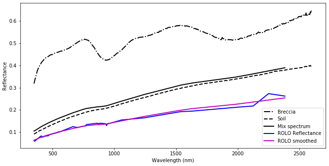
Figure 1 ROLO reflectance before and after the smoothing process, including measured spectra from the two lunar samples (breccia and soil) and the composite spectrum (adapted from Kieffer and Stone, 2005).

2.3 Developments of the ROLO model

The Global Space-based Inter-Calibration System (GSICS) developed an implementation of the ROLO model, providing an accessible tool known as GIRO (EUMETSAT, 2015). The GIRO software takes in the spectral response function of a satellite sensor, the time of observation, the position of the satellite at that time and the sensor lunar irradiance acquisition. From the time and position, it uses the NASA NAIF (Navigation and Ancillary Information Facility) SPICE tool (Acton, 1996) to calculate the selenographic coordinates (lunar phase and libration angles, g, $\mathit{\theta },\mathit{\psi },\mathit{\varphi }$) and solar and lunar distances, and the ROLO model is used to calculate the modelled lunar reflectance (from the fit parameters).

EUMETSAT has undertaken an extensive comparison between the GIRO implementation and the original ROLO implementation. The GIRO implementation was compared to the ROLO with perturbations of all input parameters, resulting in thousands of simulations. It was reported by Stone and Wagner (2018) that there were only differences related to numerical instabilities. Therefore, ROLO and GIRO can be considered identical.

Stone and Kieffer (2004) performed an assessment on the uncertainty involved in the ROLO lunar irradiance. They identified the ROLO atmospheric extinction correction algorithm as the most important source of error, accounting for the 5 %–10 % of absolute uncertainty of the irradiance model (see also Stone et al., 2020).

Lacherade et al. (2013b) observed a phase angle dependency of the ROLO calibration up to 6 % when comparing ROLO outputs and SEVIRI lunar irradiance measurements. A similar phase angle dependency between the Pléiades (Earth observation programme of the French space agency, CNES) lunar irradiances and the irradiances predicted by ROLO/GIRO was observed (Colzy et al., 2017). This phase angle dependency of GIRO was further investigated by (Barreto et al., 2016) by making aerosol optical depth (AOD) measurements from a high-altitude observatory in Tenerife, Spain, using the Cimel CE318-T radiometer, where they noted a dependence of the aerosol optical depth measurements on the lunar phase angle. It was inconclusive as to whether this systematic difference was the result of instrumental issues or inaccuracy of the ROLO model.

Other in-orbit direct measurements of lunar irradiance have also indicated a relative difference of up to 10 % in the corresponding predictions of the ROLO/GIRO model. These comparisons and applications of the current models indicate that further work is required to develop an SI-traceable absolute irradiance model of the Moon.

3 LIME overview

3.1 Overview

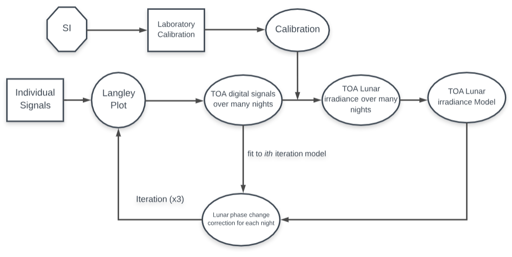
The Lunar Irradiance Model of ESA (LIME) is developed from SI-traceable observations of the Moon acquired by a Cimel CE318-TP9 radiometer from high-altitude locations, accompanied by a rigorous uncertainty analysis from calibration, through individual measurements to the model fit. Nightly top-of-atmosphere (TOA) irradiance is determined using a modified iterative Langley plot method and is fitted to a model based on the ROLO equations using specific coefficients for the Cimel spectral bands (see Sect. 6.2). Figure 2 visualises the process followed for the development of LIME.

Figure 2 Overview of the development of LIME.

3.2 Metrological approach and uncertainty analysis

A key attribute of LIME is the rigorous uncertainty analysis and the ambitious target of a sub-2 % uncertainty in the resultant model. Uncertainty contributions for each step towards the model (lunar radiometer radiometric calibration, individual measurement, derivation of TOA lunar irradiance and model fit) are considered independently, taking into account the measurement model; that is, the equation that calculates the measurand from input quantities. We then use the principles of the Guide to the Expression of Uncertainties in Measurement (the GUM JCGM, 2008) to propagate uncertainties from the laboratory calibration to the TOA lunar irradiance model parameters and output. GUM describes two methods for performing uncertainty analysis: the propagation of uncertainty and the Monte Carlo methods (JCGM101, 2008). When propagating uncertainties from radiometric calibration to nightly TOA lunar irradiance, we use the propagation of uncertainty. When considering the uncertainty in the model parameters, we use a Monte Carlo approach.

3.3 Instrument

The Cimel Electronique CE318-TP9 Sun–sky–lunar radiometer (or photometer¹) was the chosen instrument for the lunar observations. The radiometer is well known for its reliability through its use in the NASA AERONET programme (https://aeronet.gsfc.nasa.gov/ (last access: 12 March 2024); Holben et al., 1998), the globally distributed network of solar radiometers used for providing spatial and temporal extent of aerosol concentrations and properties, satellite validation, and assessing the influence of aerosols on climate change.

The CE318-TP9 is the latest version of the standard AERONET model and meets many of the requirements for low-uncertainty lunar observations. It is a multi-spectral filter radiometer which is weather-hardy and robotically pointed to acquire measurements of the Sun, Moon and sky. It has the necessary tracking capability and the dynamic range and linearity needed to cover both solar and lunar observations. It is fully automated, and day and night measurements are performed following the AERONET schedule. It comes with nine standard filters centred on 340, 380, 440, 500, 675, 870, 937, 1020 and 1640 nm and is equipped with two detectors in the sensor head: silicon and InGaAs. The 1020 nm filter is used in both the Si and InGaAs detectors for quality control purposes. It also has built-in polarisation measurement capability, with three polarisers oriented at 0, 60 and 120°.

The radiometer acquires measurement at varying electronic gains, allowing coverage of the wide dynamic range. The electronic gains are automatically set depending on the target source, so the SUN gain is the lowest and the MOON and SKY gains are the highest, with AUREOLE (for sky radiance measurement in the solar aureole) in between.

3.4 Location

To characterise the extraterrestrial irradiance of the Moon, $E_{\mathrm{0}}^{\mathrm{m}}$ , or its reflectance, A, it is essential to have as many high-quality Langley plots as possible, so it is necessary to carry out measurements at high-altitude stations (Shaw, 1979). For this reason, the Teide Peak Observatory was selected as the main measurement site for the derivation of lunar TOA irradiances. The Izaña Observatory is used as a backup station for the season of the year in which the Teide Peak Observatory is not in operation.

The Teide Peak Observatory (3555 m a.s.l.) is one of the highest-altitude stations of AERONET and is managed by the Izaña Atmospheric Research Center (CIAI; https://izana.aemet.es/, last access: 12 March 2024) from the State Meteorological Agency of Spain (AEMET). The CIAI has its own main observatory on the Izaña mountain (2401 m a.s.l.), 15 km from the Teide Peak Observatory. Both stations present optimum conditions required to derive TOA irradiance by the Langley plot method: they are located in the free troposphere with very low aerosol content, water vapour column and molecular (Rayleigh) optical depth. The low latitude (28° N) reduces the time needed to acquire Sun and Moon observations at a wide air mass range (i.e. solar elevations). Izaña also experiences 243 clear-sky days per year (Toledano et al., 2018), which is critical because even thin, high clouds significantly perturb the Langley calibration. Regarding the aerosol climatology, dominant background conditions are expected at both sites, with more than 69 % of the time under pristine conditions (AOD < 0.1 and Ångström Exponent > 0.75), as shown in Barreto et al. (2022). Only Saharan mineral dust episodes (about 20 % of days) affect these high-altitude locations, mainly in summer (July and August). Finally, the CIAI has permanent, experienced staff, as it has been involved in AERONET for more than 20 years and is accessible throughout the year. The suitability of Izaña to be an absolute calibration site by means of the Langley technique has been demonstrated in Toledano et al. (2018) and Cuevas et al. (2019). Izaña is one of the two absolute calibration sites of key photometric networks worldwide: NASA AERONET and GAW-PFR.

3.5 Strategy for extraterrestrial Moon irradiance retrieval

The classical Langley plot method is based on Beer's law (Thomason et al., 1982; WMO, 2016), which is strictly only applicable to monochromatic light but is generally accepted for narrow spectral bands with weak gas absorption. It is commonly used in the derivation of aerosol optical depth during daylight observations, where Beer’s law describes the attenuation of the Sun’s irradiance by the atmosphere.

The Langley plot method is based on the hypothesis that the properties of the atmosphere remain constant during the time needed to perform the measurements used in the linear regression, but this condition is not generally completely satisfied. To minimise the effect of changes in the atmospheric conditions, this method is better applicable if the measurements are taken at high-altitude locations, where the atmospheric attenuation and variability are low. This is a valid assumption at the Izaña and Teide Peak sites, where a Langley sequence needs about 2 h to be completed (Toledano et al., 2018). The atmospheric conditions, however, are not always optimum; thus this method results in significant variability of the retrieved lunar extraterrestrial irradiance, and it is necessary to have a large number of measurements to statistically filter out the most likely outlier values of lunar irradiance.

The difference between the application of the Langley plot method to the Sun and to the Moon is that we need to account for the continuously changing phase and libration angles of the Moon throughout the Langley period. Therefore, even when the radiometer measurements are normalised to the mean Earth–Moon and Sun–Moon distances, it is necessary to consider how the lunar extraterrestrial irradiance (and the corresponding raw measurements extrapolated at a null atmospheric optical thickness) is dependent on time, and the values obtained each night will be different.

Equation (1) is the application of Beer’s law to the photometer measurements:

$$\begin{array}{}\text{(1)}& V_{\mathrm{moon}}(\mathit{\lambda },t)=V_{\mathrm{0},\mathrm{moon}}\left(\mathit{\lambda }\right)e^{-m\left(\mathit{\theta }\right)\mathit{\tau }\left(\mathit{\lambda }\right)},\end{array}$$

where V_moon(λ,t) is the photometer output signal (in digital counts) when it measures pointing to the Moon, V_0,moon(λ) represents the lunar top-of-atmosphere signal of the photometer, m is the air mass calculated using the equation which is a function of the solar zenith angle θ in Kasten and Young (1989), and τ(λ) is the spectral total optical depth. The Langley plot method considers that the properties of the atmosphere remain constant with time; therefore τ is written as not time dependent. Taking logarithms on both sides of the Eq. (1) gives

$$\begin{array}{}\text{(2)}& \ln \left(V_{\mathrm{moon}}\right(\mathit{\lambda },t\left)\right)=\ln \left(V_{\mathrm{0},\mathrm{moon}}\right(\mathit{\lambda }\left)\right)-m\left(\mathit{\theta }\right){\mathit{\tau }}_{\mathit{\lambda }},\end{array}$$

which represents a linear relationship between ln (V_λ) and m(θ). By making observations over a relative air mass of 2–5 and fitting a straight line to the results, one can determine ln (V_0,λ), the logarithm of the top-of-atmosphere signal, as the y intercept of the linear regression of measurements vs. air mass.

The Langley plot method allows a determination of the virtually measured top-of-atmosphere signal of the photometer by effectively correcting the effect of the atmospheric extinction on the ground measurements. In this way, it is not necessary to know a priori the gas and aerosol extinction, which is general unknown. Thus, for each suitable night, extraterrestrial lunar irradiance for a specific phase angle is obtained.

To account for the change in lunar irradiance due to minute changes in phase angle during the Langley period, the typical Langley plot method is modified to include an iterative step. Figure 3 outlines this iterative process. In the first iteration, it is considered that the top-of-atmosphere irradiance of the Moon remains constant during the Langley measurements. Applying this approach to the complete set of night data (several years of measurements), a first estimation of the lunar reflectance, A, is obtained. These first reflectance values are used to adjust a lunar reflectance model, based on the ROLO equations, in order to have an estimation of the lunar irradiance change during the Langley measurements in the next iteration. This first estimate of the lunar reflectance model is used to perform a new set of nocturnal Langley plots, this time taking into account the phase change of the Moon irradiance along the Langley duration, using the correction

$$\begin{array}{}\text{(3)}& V^{\prime }(\mathit{\lambda },t)=V(\mathit{\lambda },t){\displaystyle \frac{A(t_{\mathrm{ref}},\mathit{\lambda })}{A(t,\mathit{\lambda })}},\end{array}$$

where V and V^′ are the photometer signal before and after phase change correction and t_ref is the mean time of each Langley plot (thus the time corresponding to V_0,moon from each Langley fit). The iterative process converges rapidly, so only three iterations are required. Finally, a corrected set of lunar TOA irradiances and phase angles is obtained.

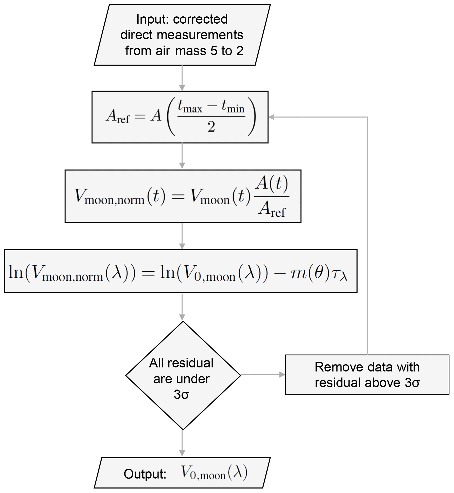
Figure 3 Iterative correction scheme of TOA irradiance over a Langley period (single-night Moon observations).

4 Calibration

Many current post-launch satellite calibration systems are not traceable to SI (Bouvet et al., 2019). In the development of LIME, this issue is addressed by deriving the model from SI-traceable observations through the photometer irradiance calibration performed at the National Physical Laboratory (NPL).

A detailed characterisation of the lunar photometer was performed and accompanied by a rigorous uncertainty analysis following metrological principles. The characterisation included an assessment of linearity across the wide dynamic range of signal expected across the lunar cycle, thermal sensitivity characterisation of the instrument to determine corrections to apply to data obtained at a wide range of ambient temperatures and spectral irradiance calibration coefficients for each spectral channel of the instrument.

4.1 Linearity

For the Cimel photometer to measure the signal range over the lunar phase and librations, the instrument has a wide dynamic range. It was necessary to perform tests to ensure it had a linear response over this range. These tests were performed at the NPL linearity facility using best practice for linearity characterisation, the double-aperture method (Theocharous, 2012). This is based on the superposition principle.

The NPL facility used a double-aperture linearity wheel and neutral-density filters to vary the levels of radiation. The facility is fully automated and allows the testing of the linear response of a detector over the spectral range of 200 nm to 20 µm (depending on the light source used).

The double-aperture wheel was set into four different positions during the measurements, where for position A and B respectively the bottom or top half on the illumination beam was baffled, the A + B position gave the full light reading, and D was the external dark reading. A tungsten strip lamp was used as a source. Measurements were repeated a number of times, and each sequence consisted of a dark reading, an A reading, a B reading and an A + B reading and then of a B reading, an A reading and a dark reading in the end. For a linear response we would expect the signal when both the apertures are open to equal the sum of the signal through each aperture individually. A linearity factor, L(V_A + B), was then calculated using Eq. (4).

$$\begin{array}{}\text{(4)}& L\left(V_{\mathrm{A}+\mathrm{B}}\right)={\displaystyle \frac{V_{\mathrm{A}+\mathrm{B}}}{(V_{\mathrm{A}}+V_{\mathrm{B}})}}.\end{array}$$

A linearity factor was calculated for illumination levels varied by changing neutral-density filters, covering the typical signal range from lunar measurements at high phase angles (about 200–3000 counts depending on wavelength) up to direct solar measurements near noon (about 100 000 counts). Then the results were averaged for the final estimation of linearity for each Cimel spectral channel. For wavelengths of 500 nm and beyond, the non-linearity was observed to be less than 0.1 % with a standard deviation of values for different levels of less than 0.1 %, and the results show no systematic pattern (Fig. 4). Therefore, non-linearity was considered negligible here. At shorter wavelengths, any non-linearity was indistinguishable from the noise.

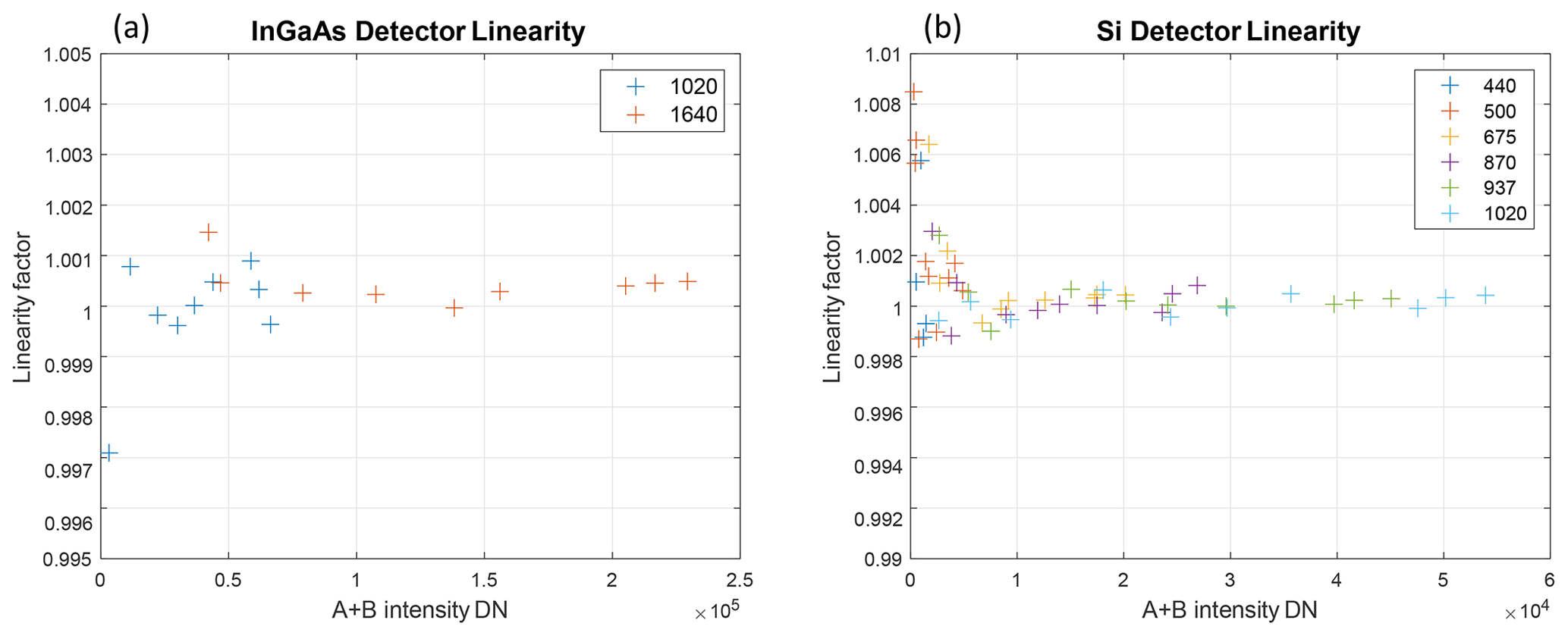
Figure 4 Linearity results for the InGaAs detector (a) and for the Silicon detector (b) of the Cimel radiometer.

4.2 Temperature sensitivity

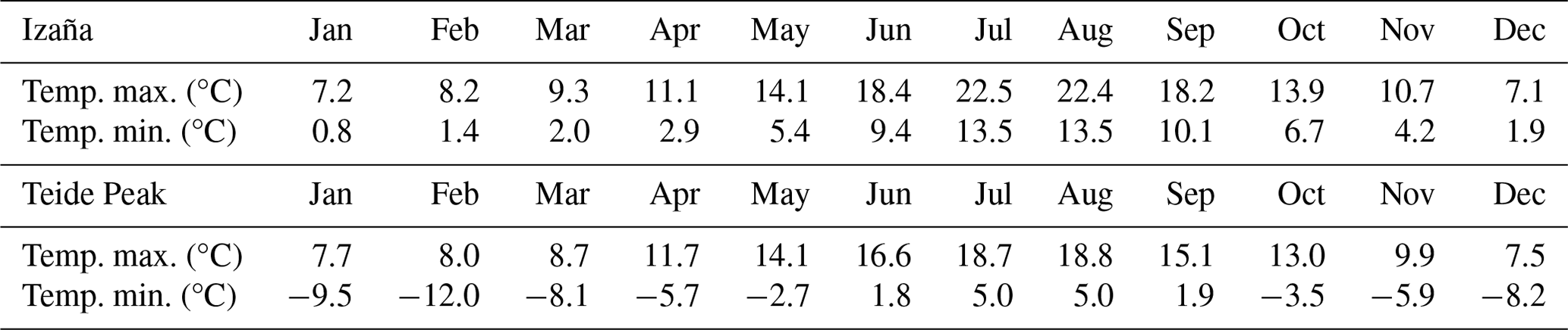
The temperatures at the observation sites vary significantly between the two sites and seasonally (Table 1). As the instrument is not thermally stabilised, its thermal sensitivity was assessed to determine temperature correction to compensate for the effect of the temperature variation during the realisation of day and night Langley plots. This is particularly important for 1020 nm, where the silicon detector is particularly temperature-sensitive, but is also necessary to determine for all spectral channels.

Table 1 Monthly maximum and minimum daily mean temperatures for the Izaña station (upper table) in the period 1971–2000 and for Teide Peak (lower table) from 2013–2016 (in this case, preliminary statistics).

The temperature sensitivity was characterised at the University of Valladolid in a Climats thermal chamber. This consists of a stainless-steel cabinet with a gridding where the photometer can be positioned, and the right side has an 80 mm diameter aperture. The photometer is aligned with an integrating sphere (Labsphere 10 in. diameter), illuminated with a 100 W lamp and powered by a stabilised power supply (Agilent E3634A). We carried out two independent tests where the lunar photometer sensor head performed measurements on the MOON gain scenarios at temperatures ranging from +50 to −40 °C during a period of 4 h, which is a rate of change of about 0.3 °C min⁻¹.

The irradiance, E_T, was measured in the temperature chamber at different temperatures, T[°C], while the detector was illuminated with a stable light source. The acquired data were then fitted to the following model:

$$\begin{array}{}\text{(5)}& E_T=E+c_{\mathrm{1}}(T-T_{\mathrm{ref}})+c_{\mathrm{2}}(T-T_{\mathrm{ref}}{)}^{\mathrm{2}},\end{array}$$

where T_ref is the reference temperature (25 °C) and E is the irradiance of the sources measured at the reference temperature. The measurements for all spectral channels in the range of 440–1640 nm are shown in Fig. 5.

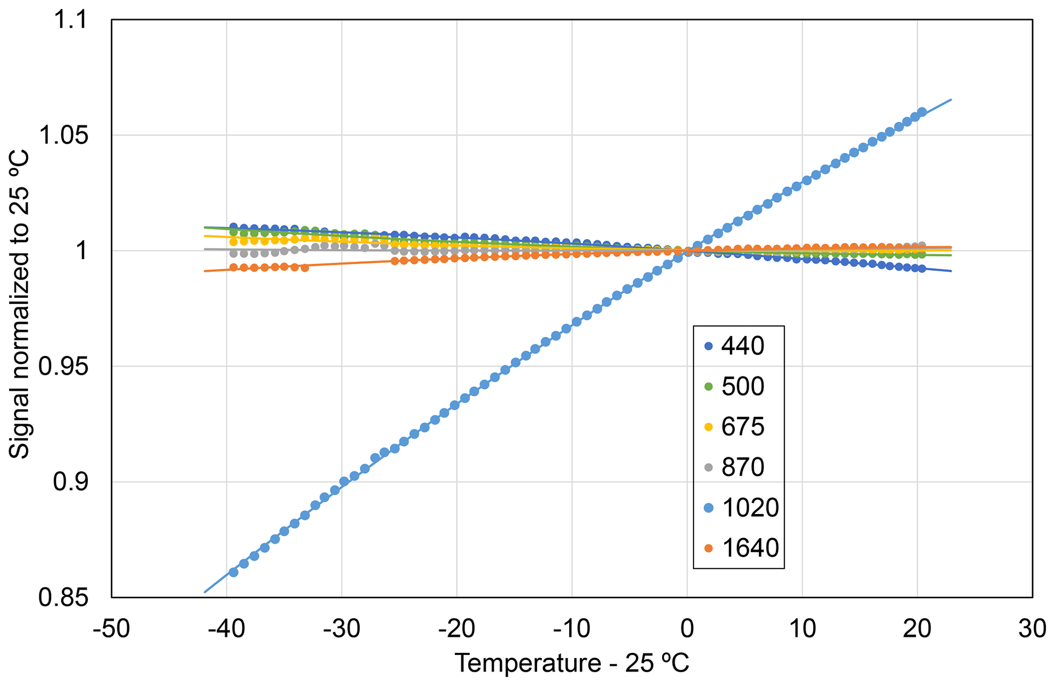
Figure 5 Observed temperature sensitivity plot for the lunar photometer channels (440 to 1640 nm), where the signals have been normalised to the value at 25 °C.

The coefficients c₁ and c₂ were then used in a temperature correction factor (Eq. 6) which is applied to all lunar measurements, correcting for the differing temperatures during observation. The temperature corrections F_T,i for the spectral channel i were applied to the raw data used to determine the spectral irradiance and radiance calibration coefficients at the NPL.

$$\begin{array}{}\text{(6)}& F_T=[\mathrm{1}+c_{\mathrm{1},i}(T-T_{\mathrm{ref}})+c_{\mathrm{2},i}(T-T_{\mathrm{ref}}{)}^{\mathrm{2}}]\end{array}$$

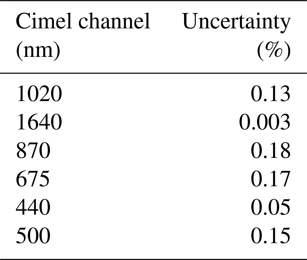
Uncertainties associated with the temperature sensitivity coefficients derived from a measurement sequence are very small. Therefore, we repeated the measurements in the thermal chamber and compared the two sets of temperature sensitivity coefficients. The difference between the temperature corrections associated with each set of coefficients was calculated. This difference is temperature-dependent and is zero for the reference temperature (25 °C). In order to provide example uncertainties, the difference between the correction calculated with each set of coefficients was determined at 11.3 °C, as that is the mean temperature during Langley plots at the Izaña Observatory from June 2014 to October 2017. The values are given in Table 2. We consider this a better estimation of the uncertainty in the temperature correction, as it involves the repeatability of the entire thermal characterisation.

Table 2 Estimates of the relative uncertainty associated with the temperature correction for irradiance measurements in each lunar photometer spectral channel.

4.3 Spectral irradiance responsivity

The irradiance responsivity of each lunar photometer spectral channel was assessed at the NPL by measuring the response of each of the detectors in turn with two different sources of known irradiance at a variety of distances to ensure the wide dynamic range required for the lunar observations was covered.

Irradiance sources calibrated at the NPL are traceable to the primary standard, the cryogenic radiometer where electrical power is compared to optical power in a cryogenic blackbody cavity. The calibration is then transferred via a laser to a trap detector (an arrangement of Si photodiodes that reduce signal loss by reflectance to negligible levels). This in turn is used to calibrate a filter radiometer, which measures the radiance of a 3000 K blackbody source in the spectral band of the filter. From this and Planck’s law, the temperature of the blackbody, and hence the radiance at other temperatures, is known accurately. With an appropriate geometric system consisting of two apertures, the radiance of the blackbody can be compared directly to the irradiance of an FEL lamp at 500 mm from the reference frame, using a monochromator to measure each wavelength. The FEL lamp is therefore a reference source of known spectral irradiance and was used in the Cimel calibration as the calibrated reference source. To achieve lunar irradiance levels, a transfer radiometer was used to step down to a lower power source.

The calibration coefficient for each spectral band was determined by Eq. (7):

$$\begin{array}{}\text{(7)}& C_{\stackrel{\mathrm{‾}}{E},\mathrm{Cimel}}\left({\mathit{\lambda }}_i\right)={\displaystyle \frac{\left({\sum }_j{E}_{\mathrm{lamp},x}\right({\mathit{\lambda }}_j\left){\mathit{\xi }}_j\right({\mathit{\lambda }}_j\left)\mathit{\delta }\mathit{\lambda }\right)F_T}{G_{\mathrm{ratio}}\left[V_{\mathrm{Cimel},\mathrm{lamp},x}\right({\mathit{\lambda }}_i)-V_{\mathrm{Cimel},\mathrm{dark}}({\mathit{\lambda }}_i\left)\right]}}+\mathrm{0},\end{array}$$

where $C_{\stackrel{\mathrm{‾}}{E},\mathrm{Cimel}}\left({\mathit{\lambda }}_i\right)$ is the band-integrated irradiance calibration coefficient for band i of the lunar photometer at wavelength λ, E_lamp,x(λ_j) is the irradiance of the lamp at wavelength λ and distance x, ξ_j(λ_j) is the normalised (for unit area) spectral response function at wavelength λ_j defined at equispaced wavelengths separated by δλ, F_T is the temperature correction from the calibration instrument temperature to the nominal reference temperature of 25 °C, and G_ratio is the gain ratio from the gain of measurement (e.g. SUN or AUR) to the MOON gain. Depending on the measurement target, the photometer switches the electronic gain automatically. The linearity was characterised for all gain settings (Sect. 4.1). The nominal values are

$$\begin{array}{}\text{(8)}& {\displaystyle \frac{C_{\mathrm{SUN}}}{C_{\mathrm{MOON}}}}=\mathrm{4096};{\displaystyle \frac{C_{\mathrm{AUR}}}{C_{\mathrm{MOON}}}}=\mathrm{32}.\end{array}$$

$V_{\mathrm{Cimel},\mathrm{lamp},x}\left({\mathit{\lambda }}_i\right)$ is the Cimel signal for channel at wavelength λ when looking at the lamp at distance x; V_Cimel,dark(λ_i) is the dark signal for channel at wavelength λ; and 0 represents the approximations in the form of the equation, in particular, that the Cimel is linear and that the summation on the numerator is an appropriate approximation for the spectral integral. This follows notation used in Mittaz et al. (2019).

4.4 Calibration uncertainty analysis

As described in Sect. 3.2, rigorous uncertainty analysis was a key attribute of LIME, where the target is to reach an uncertainty < 2 % in the resultant model. By calibrating the lunar photometer, traceable to the primary standard of the cryogenic radiometer at the NPL, low uncertainty in the photometer calibration was achievable. The uncertainty analysis for the radiometric calibration followed the principles in GUM (JCGM, 2008), using propagation of uncertainty.

Propagation of uncertainty applies a locally linear approximation to the measurement function f and propagates standard uncertainties (the standard deviation of the probability distribution from which the unknown measurement error is drawn) through this approximation. It can be written as a summation as

$$\begin{array}{}\text{(9)}& u_c^{\mathrm{2}}\left(y\right)=\sum _{i=\mathrm{1}}^n{\left({\displaystyle \frac{\partial f}{\partial x_i}}\right)}^{\mathrm{2}}{u}^{\mathrm{2}}\left(x_i\right)+\mathrm{2}\sum _{i=\mathrm{1}}^{n-\mathrm{1}}\sum _{j=i+\mathrm{1}}^n{\displaystyle \frac{\partial f}{\partial x_i}}{\displaystyle \frac{\partial f}{\partial x_j}}u(x_i,x_j),\end{array}$$

where $u_c^{\mathrm{2}}\left(y\right)$ represents the combined variance, the first term adds the uncertainty contributions from the input quantities in quadrature and the second term deals with error correlation (common errors) between the different input quantities. The partial derivatives $\left(\partial f/\partial x_i\right)$ are the sensitivity coefficients, which convert an uncertainty associated with the input quantity x_i into an uncertainty associated with the measurand. The term u(x_i,x_j) is the covariance associated with pairs of input quantities.

It was important to distinguish “common uncertainties” from “common errors”. Two measurements at different distances may have a common uncertainty associated with noise, but they will have different errors. On the other hand, the uncertainty associated with lamp calibration will have a common error at the two different distances. By considering what is common and what changes from one measurement to another, we can get a meaningful uncertainty associated with an average of those measurements: the uncertainties associated with effects that have common errors will not reduce on averaging, and those associated with effects whose error changes will reduce on averaging.

The irradiance responsivity was measured at the NPL using several methods in order to cover the range of signal levels appropriate for the lunar observations, as described in Sect. 4.3. The band-integrated irradiance calibration coefficient was determined for each method at varied lamp–photometer distance along with an associated uncertainty.

We consider for each method the measurement model, the general form applicable to each method given in Eq. (7). The uncertainty for each term in the measurement model and its magnitude was determined and then categorised by the following error correlation structures:

• a.

  Fully independent uncertainties corresponding to errors (e.g. noise) which vary from observation to observation (i.e. are different at different distances and for the different methods).

• b.

  Fully common uncertainties (e.g. SRF) where the error is (almost) identical for all measurements with all sources at all distances.

• c.

  Lamp uncertainties (e.g. their calibration) where the error is common to all methods that use the same lamp.

• d.

  Method-common uncertainties where the error is common to the measurements at different distances with this method but is different for other methods.

All the considered uncertainty sources in the calibration of the lunar photometer are provided in Table 3. The final calibration coefficients and their associated standard (k=1) and expanded (k=2) uncertainties are given in Table 4.

Table 3 Uncertainties associated with the calibration of the lunar photometer. See text for the description of categories “a”, “b”, “c” and “d” of error correlation structures.

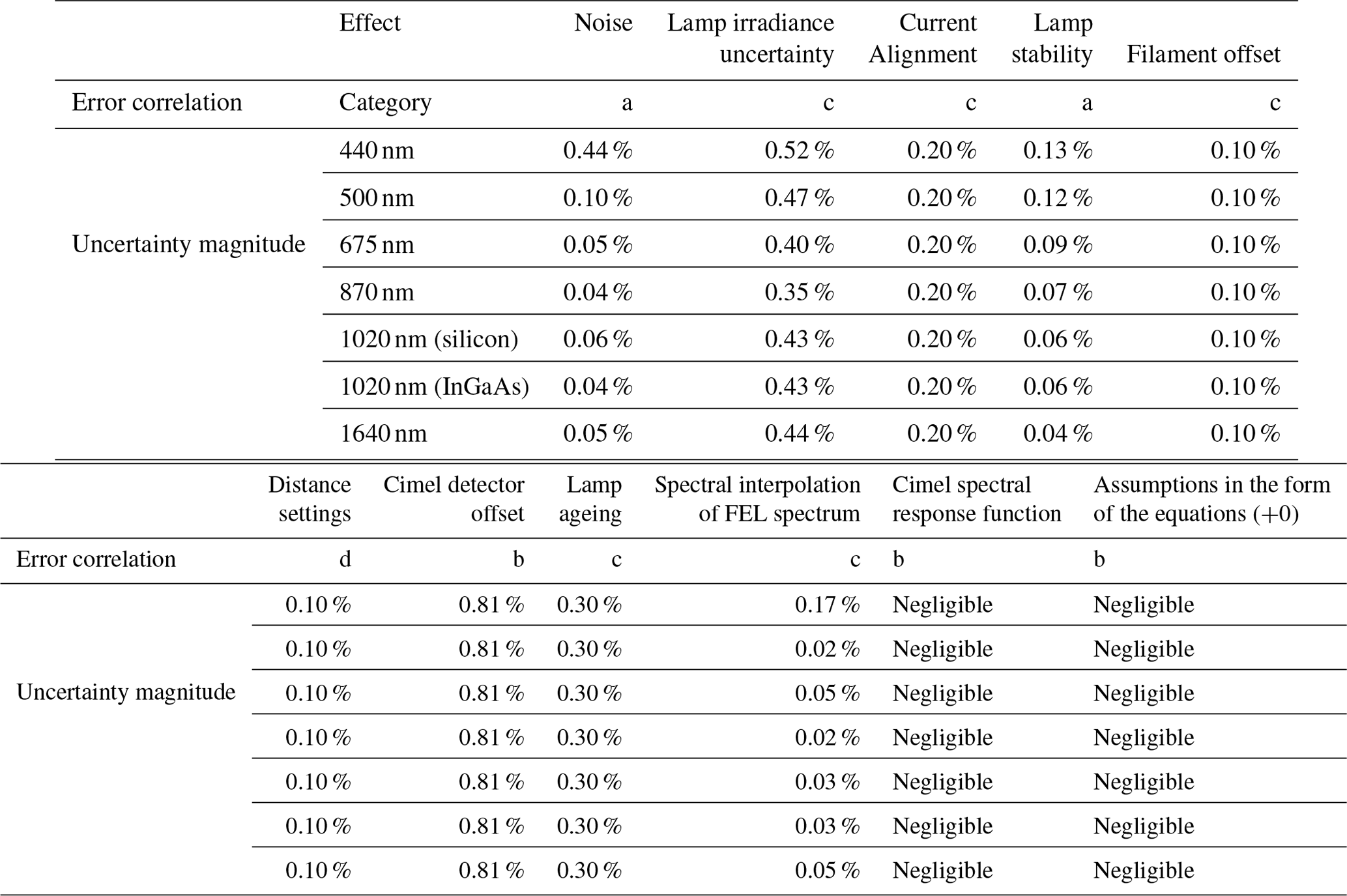
Table 4 Calibration coefficients for each Cimel photometer spectral band used in LIME and associated uncertainty.

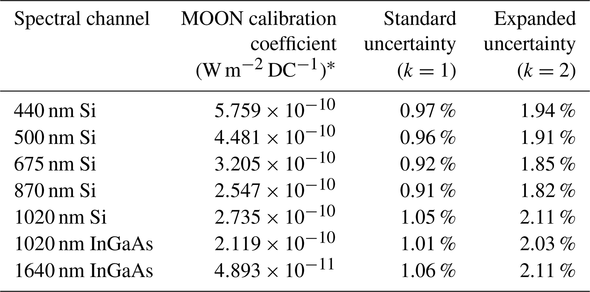
^*DC stands for instrument signal in digital counts units.

5 Derivation of nightly TOA lunar irradiance and associated uncertainty

Top-of-atmosphere lunar irradiance is determined each night through lunar phase angles spanning from −90 to +90° by acquiring a large number of measurements over a relative air mass of 2–5 (lunar zenith angles between 60 and 78°) and determining TOA signal using the Langley plot method. Observations were made at the Izaña Atmospheric Observatory in the colder winter months and at the Teide Peak in the summer.

5.1 Measurement acquisition details and data processing

The ESA lunar photometer (Cimel with serial number 1088) has been installed and operational since March 2018. In the current iteration of LIME, the instrument has provided approximately 590 nights of lunar acquisitions suitable for Langley plots over more than 5 years of measurements. On 60 % of the days the photometer has operated at Izaña, whereas on 40 % of the days it has operated at Teide Peak.

As well as the ESA lunar photometer, another instrument (“master” instrument with serial number 933) has been acquiring lunar observations over a period of 9 years, providing more than 1100 acquisitions. The concurrent operation of this and other reference (“master”) photometers at the Izaña site provides an opportunity for monitoring the stability of the ESA photometer between laboratory calibrations. A careful comparison between both instruments was carried out in the framework of the LIME project (https://calvalportal.ceos.org/lime-documents, last access: 12 March 2024). These comparisons, together with the analysis of solar Langley plots, reveal a very small instrument drift, ranging from −0.1 % for the SWIR channels and up to −0.8 % for the 440 nm channel, over more than 4 years of operation.

The instrument's direct lunar observations consist of groups of three acquisitions (dark current is automatically subtracted) within a 1 min interval for all spectral channels. The CÆLIS software tool (Fuertes et al., 2018) is used to automatically digest those data and produce the Langley plot (see Sect. 3.5) plus some statistical indicators of the fit quality, including the uncertainty of the y intercept (see Sect. 5.3.2). Lunar zenith angles and Earth–Moon–Sun distances are obtained from the SPICE astronomic library. CÆLIS also produces real-time data flags according to the meta-data provided by the Cimel instrument, aerosol optical depth and precipitable water vapour (González et al., 2020). All this information is used to monitor the instrument performance on a daily basis.

5.2 Deriving lunar irradiance from observations

SI-traceable Lunar extraterrestrial irradiance, $E_{\mathrm{0},\mathrm{moon}}(\mathit{\lambda },t)$, was determined on each night of observation multiplying lunar top-of-atmosphere signals of the photometer, $V_{\mathrm{0},\mathrm{moon}}(\mathit{\lambda },t)$, obtained by the nocturnal Langley plots, by the absolute radiometric calibration coefficient, $C_{\stackrel{\mathrm{‾}}{E},\mathrm{Cimel}}\left({\mathit{\lambda }}_i\right)$ determined in the characterisation carried out at the NPL facilities, as described in Sect. 4.3:

$$\begin{array}{}\text{(10)}& E_{\mathrm{0},\mathrm{moon}}(\mathit{\lambda },t)=V_{\mathrm{0},\mathrm{moon}}(\mathit{\lambda },t)C_{\stackrel{\mathrm{‾}}{E},\mathrm{Cimel}}\left({\mathit{\lambda }}_i\right).\end{array}$$

Additionally, the lunar-disc-equivalent albedo, A, or more briefly the lunar reflectance, was also determined. A, is defined as follows:

$$\begin{array}{}\text{(11)}& A(\mathit{\lambda },t)={\displaystyle \frac{E_{\mathrm{0},\mathrm{moon}}(\mathit{\lambda },t)\cdot \mathit{\pi }}{{\mathrm{\Omega }}_{\mathrm{moon}}{E}_{\mathrm{0},\mathrm{sun}}\left(\mathit{\lambda }\right)}},\end{array}$$

where E_0,moon is the lunar extraterrestrial irradiance, E_0,sun is the solar extraterrestrial irradiance and Ω_moon is the solid angle of the Moon at mean distance (384 400 km), which takes a value of $\mathrm{6.4177}\times {\mathrm{10}}^{-\mathrm{5}}$ sr. The TSIS-1 solar spectrum (Coddington et al., 2021) is used for this purpose.

5.3 TOA lunar irradiance measurement uncertainty analysis

The uncertainty analysis for the individual measurements contributing to the Langley plots, and subsequent derivation of the nightly TOA irradiance, follows the law of propagation of uncertainty, as described in Sect. 4.4. In this analysis we only consider the final iteration of the Langley plots.

In the determination of the lunar irradiance, error correlation is important in two places: first, when one makes a Langley plot and fits a straight line through data points made from individual observations of the Moon over a single night. While each measurement point will have an individual noise error (noise errors vary on timescales faster than the measurement time), other errors may be common from one measurement to another. For example, instrument calibration errors will apply to all measured values, and slowly varying atmospheric conditions can create a measurement error that is correlated for measurement points close together in time. These correlations must be considered to obtain the right uncertainty associated with the model.

Following the same principles outlined in the uncertainty analysis for the calibration, we begin by considering the measurement models.

5.3.1 Individual observations in situ

An individual measurement that goes into the Langley plot consists of a pair of airmasses, m(θ), and a count signal $V^{\prime }(\mathit{\lambda },t)$.

$$\begin{array}{}\text{(12)}& V^{\prime }(\mathit{\lambda },t)={\displaystyle \frac{V(\mathit{\lambda },t)}{F_T\left(\mathit{\lambda }\right)}}{\displaystyle \frac{A(t_{\mathrm{ref}},\mathit{\lambda })}{A(t,\mathit{\lambda })}}{K}_{\mathrm{dist}}+\mathrm{0},\end{array}$$

where F_T(λ) is the temperature correction factor described in Sect. 4.2.

K_dist is a correction for the actual Sun–Moon and Earth–Moon distances x relative to the standard distances:

$$\begin{array}{}\text{(13)}& K_{\mathrm{dist}}={\left({\displaystyle \frac{x_{\mathrm{sun}-\mathrm{moon}}}{\mathrm{1}\left[\mathrm{au}\right]}}\right)}^{\mathrm{2}}{\left({\displaystyle \frac{x_{\mathrm{earth}-\mathrm{moon}}}{\mathrm{384000}\left[\mathrm{km}\right]}}\right)}^{\mathrm{2}},\end{array}$$

and A(t_ref,λ) and A(t,λ) are used to correct for the lunar phase change during the Langley period as described in Sect. 3.5. The term “+0” represents the assumptions built into the form of the equations. For a single measurement this includes the assumption of instrument linearity.

The air mass m(θ), Eq. (14), is calculated using equations in Kasten and Young (1989) . It is a function of the lunar zenith angle and takes a slightly different form for ozone and nitrous oxide to that for aerosols. The combined air mass is used here:

$$\begin{array}{}\text{(14)}& m=\mathrm{1}/(\cos \mathit{\theta }+\mathrm{0.50572}(\mathrm{96.07995}-\mathit{\theta }{)}^{-\mathrm{1.6364}}),\end{array}$$

where the zenith angle θ is expressed in degrees.

The relative air mass range is restricted to 2–5, thereby avoiding errors in optical air mass determination that increases significantly at larger zenith angles (Russell et al., 1993). For uncertainty purposes, the uncertainty associated with the air mass is considered negligible.

The uncertainty associated with the temperature correction is outlined in Sect. 4.2.

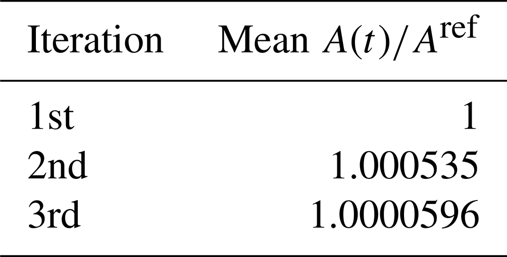
The correction applied for change of lunar phase and libration angles during the Langley plots normalises the lunar direct measurements using the ratio of the lunar reflectance at a specific time, A(t), to the lunar reflectance at the Langley mean time, A^ref . In order to obtain this parameter a first approximation of a lunar reflectance model is used, as described in Sect. 3.5, so this is done in an iterative process. In the first iteration, $A\left(t\right)/A^{\mathrm{ref}}$ is considered equal to 1, and a parametric model is fitted to the retrieved lunar reflectance. The model obtained in one iteration is used in the following iteration. The uncertainty associated with the final $A\left(t\right)/A^{\mathrm{ref}}$ ratio is evaluated as the difference between the ratios of the last and the penultimate iterations. Using the measurements taken at the Izaña Observatory from June 2014 to October 2017, the mean $A\left(t\right)/A^{\mathrm{ref}}$ ratio for three iterations was calculated (Table 5). The difference between the second and third iterations is as low as $\mathrm{6}\times {\mathrm{10}}^{-\mathrm{5}}$, equivalent to an uncertainty of 0.006 %.

Table 5 Mean $A\left(t\right)/A^{\mathrm{ref}}$ for three iterations using the measurements obtained at the Izaña Observatory from June 2014 to October 2017.

Because of the complexity of processing data within the SPICE system used in the distance correction, the Jet Propulsion Laboratory (JPL) does not provide numerical mechanisms for managing uncertainty information. In this correction we have used the high-accuracy lunar orientation data (MOON_ME or Moon Mean Earth/Rotation axis frame) as a reference. The only reference in the SPICE system about uncertainty in distances is related to the standard low-accuracy reference model (IAU_MOON), which is expected to have an associated uncertainty of 0.0051° or 155 m on a great circle in the worst case and 0.0025° or 76 m on average. Even if these values are considered (being rather conservative), we consider this a negligible error (NAIF, 2018).

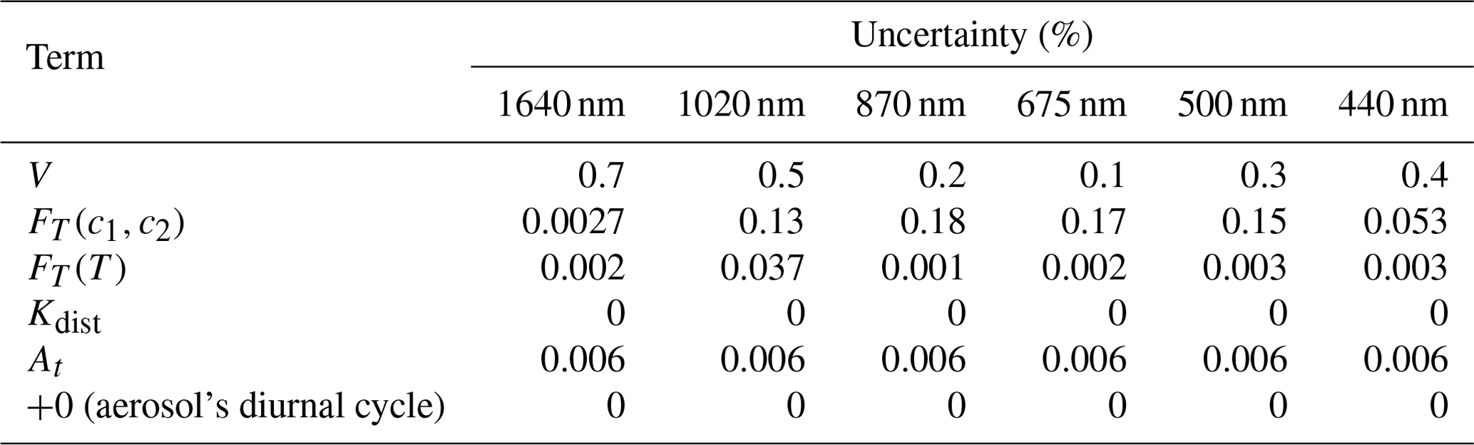
Each uncertainty source contributing to individual observations, along with the error correlation structures, is summarised in Table 6; the percentage uncertainty arising from each source of uncertainty at each photometer band is presented in Table 7.

Table 6 Summary of sources of uncertainty for individual lunar observations, i.e. raw signals per photometer spectral band. Note that n/a indicates not applicable.

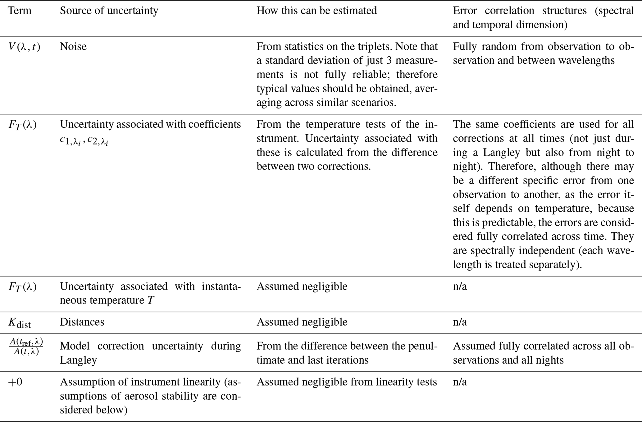
Table 7 Percentage uncertainty arising from each source of raw signal uncertainty (see Table 6) at each Cimel photometer band.

5.3.2 Uncertainty associated with the Langley plots

We also consider the uncertainty associated with the least-squares fit in the Langley plot, where we take into account the uncertainty associated with each data point and determine an uncertainty associated with the y intercept, ln (V_0,λ), which is the logarithm of the TOA signal.

Each data point was given the same relative uncertainty, taken from the standard deviation of the triplets (three individual acquisitions within 1 minute), V(λ,t); see Table 7. A straight-line fit based on ISO/TS_28037:2010 (2010) was used to calculate the uncertainty associated with the y intercept of the linear fit (see Fig. 6) and the χ² of the fit and then validated it using the χ² test. Where the observed χ² was smaller than the 95 % quantile of expected ${\mathit{\chi }}_{\mathit{\nu }}^{\mathrm{2}}$ for the degrees of freedom of a given Langley plot (where degrees of freedom, ν, are defined as n-2 and n is the number of measurements used to obtain the Langley plot), the intercept uncertainty was accepted. Where the observed χ² was larger than the 95 % quantile of expected ${\mathit{\chi }}_{\mathit{\nu }}^{\mathrm{2}}$, the relative uncertainty on each data point was increased by small increments until the χ² test was passed (Fig. 7).

When performing the fit and applying the χ² test, very few of the Langley plots passed using the original uncertainty on the input parameters. This indicated a potential underestimation of the uncertainty associated with the Langley plots. This could likely be the result of small changes in aerosol (and other atmospheric) properties during the Langley period. It is also reasonable to assume that using a standard deviation of the triplets, which shows instrument stability over a very short period, underestimates the uncertainty associated with the stability of the instrument for the duration of the Langley. For those that failed the χ² test, uncertainty on input parameters was increased incrementally until the test was passed and uncertainty associated with the y intercept, ln (V₀) was determined (Fig. 7b). A small selection required a small increase in uncertainty for each data point, and a few had high uncertainty, indicating that the fit should be considered for removal from the data set or have very low weighting in the final model.

Figure 6 Examples of Langley plots which pass the χ² test.

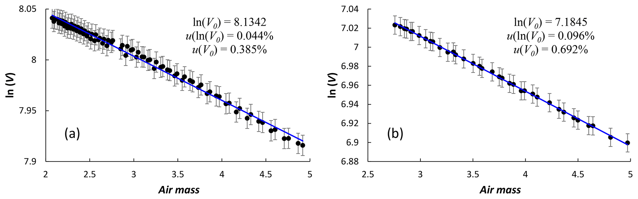
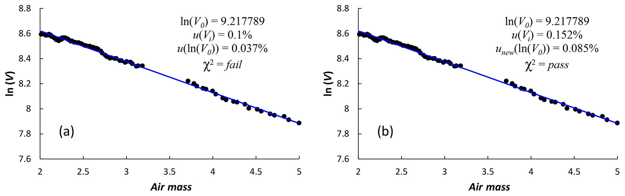
Figure 7 Langley before (a) and after (b) increase in uncertainty in order to pass the χ² test.

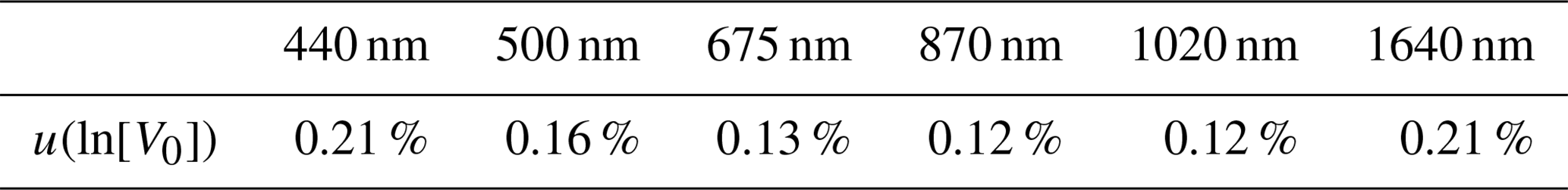
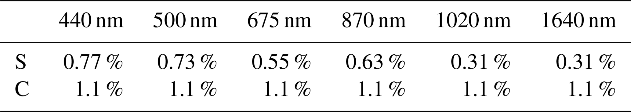
Using the values of u(ln [V₀]) and the u_new(ln [V₀]) where appropriate, a “typical” uncertainty associated with the y intercept of the Langley plots was determined and used in the Monte Carlo uncertainty analysis (MCUA) input parameters for the model fit uncertainty analysis (see Sect. 6.4). The values are provided in Table 8. They are in the range of 0.1 %–0.2 %, lower for longer wavelengths except for the 1640 nm channel.

Table 8 Estimated uncertainty in the y intercept of the Langley plots for each Cimel photometer spectral band.

6 LIME

6.1 Model concept

The model is derived from the lunar irradiance measurements from the Cimel photometer. It is based on a slightly modified version of the ROLO lunar model described in Sect. 2.1. The modification in LIME is that, for each spectral band in the model, an independent set of c coefficients has been defined, while in the original model, the c coefficients are identical for all bands. Then the lunar reflectance A for each photometer spectral band k is modelled as follows:

$$\begin{array}{}\text{(15)}& \begin{array}{rl}\ln \left(A_k\right)& =\sum _{i=\mathrm{0}}^{\mathrm{3}}{a}_{ik}{g}^i+\sum _{i=\mathrm{1}}^{\mathrm{3}}{b}_{ik}{\mathrm{\Phi }}^{\mathrm{2}i-\mathrm{1}}+c_{\mathrm{1}k}\mathit{\theta }+c_{\mathrm{2}k}\mathit{\varphi }\\ & +c_{\mathrm{3}k}\mathrm{\Phi }\mathit{\theta }+c_{\mathrm{4}k}\mathrm{\Phi }\mathit{\theta }+d_{\mathrm{1}k}\exp \left({\displaystyle \frac{-g}{P_{\mathrm{1}}}}\right)\\ & +d_{\mathrm{2}k}\exp \left({\displaystyle \frac{-g}{P_{\mathrm{2}}}}\right)+d_{\mathrm{3}k}\cos \left({\displaystyle \frac{g-p\mathrm{3}}{p\mathrm{4}}}\right),\end{array}\end{array}$$

where ln (A) is the natural logarithm of A, g is the absolute phase angle [radians], θ is the selenographic latitude of the observer [degrees], ϕ is the selenographic longitude of the observer [degrees], and Φ is the selenographic longitude of the Sun [radians].

The reflectance model can be split into four different sections. The basic photometric function is represented by the first polynomial depending solely on the phase angle. It is a wavelength-dependent third-degree polynomial, described with the $a_k^i$ coefficients. The variations in the reflectance of the Moon due to changes in the actual area of the Moon illuminated by the Sun and driven by changes in the distribution of maria and highlands is expressed in the second polynomial. This polynomial depends only on the solar selenographic longitude Φ. Fourth-order coefficients b_ik are defined for every wavelength. The third section, with four wavelength-dependent coefficients c_ik, represents the visible part of the Moon and how it is illuminated (topographic libration). The last part of the equation is a set of parameterised exponential and cosine functions modulated by a set of d_ik coefficients: it is an empirical iterative least-squares fitting of non-linear residuals in the irradiance with respect to the phase angle.

6.2 Initial model fit at the photometer spectral bands

The strategy designed to calculate the model coefficients is divided into different steps (Fig. 8), taking the lunar measurements restricted to the phase angle interval [−90°, 90°] and the geometric calculation as a starting point. The calculation of the observer, lunar and solar geometries is done by the application of the CSPICE library, provided to the public by NASA NAIF (Acton, 1996; Acton et al., 2018).

Figure 8 Scheme of the lunar model coefficients regression algorithm.

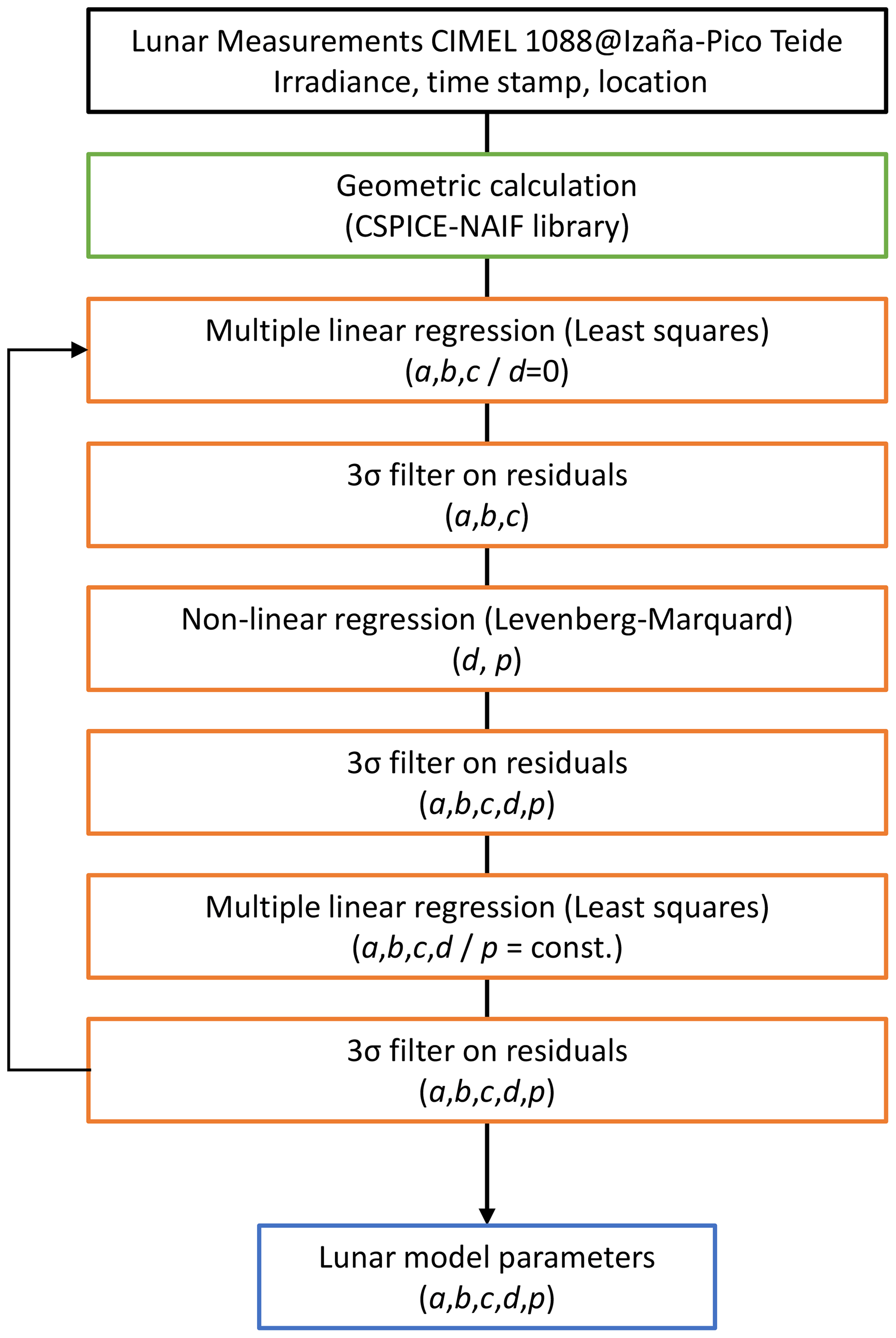
A least-squares fit is used to derive those coefficients belonging to the linear part of the model, i.e. band-specific a, b and c coefficients in Eq. (15). All d parameters are set to zero in this first approximation. A subsequent regression is performed on the non-linear part of the equation using the Levenberg–Marquardt method, taking into account that this non-linear part of the lunar reflectance model depends on the measurement phase angle. Therefore, d and p parameters are calculated from the residuals calculated with previous steps. For convenience in the first iteration, all a parameters will be fitted against all bands. In the second iteration the p parameters are adopted from the first fitting. From that point, the band-specific d parameters are re-fitted in a linear least squares with all a, b and c parameters. The p parameters are then used in further regression and outlier removals. Finally, again, a full linear fitting is performed on the entire equation, keeping the previously derived non-linear parameters constant (p parameters). It is important to note that a 3σ outlier removal (based on the standard deviation of the residuals) is applied after all regression steps to ensure the quality of the whole fitting analysis.

6.3 Uncertainty analysis

The lunar model fit is a multi-step process as described in Sect. 6.2, where the linear part of the model is fitted for each band, the outlier is removed, then the non-linear part is fitted. This is followed by further outlier removal, and, finally, the linear part is fitted again. The whole multi-step process is itself iterated.

The approach to uncertainty analysis in the model regression follows the Monte Carlo uncertainty analysis (MCUA) methods outlined in GUM (JCGM101, 2008). The Monte Carlo analysis is fed with simulated random errors based on the knowledge of uncertainties provided with the measurements. In practice, every measurement is slightly adjusted with a simulated random error that is taken from a distribution (usually normal) with a standard deviation given by the standard uncertainty. The MCUA process is based on a statistical measurement model. The input irradiance values (the TOA irradiance values for each night obtained by the Langley method) are treated as

$$\begin{array}{}\text{(16)}& E_{i,\mathit{\lambda }}=E_{i,\mathit{\lambda }}^{\mathrm{True}}\cdot (\mathrm{1}+R_{i,\mathit{\lambda }})(\mathrm{1}+S_{\mathit{\lambda }})(\mathrm{1}+C),\end{array}$$

where $E_{i,\mathit{\lambda }}^{\mathrm{True}}$ is the nominal “true” value for the TOA irradiance in spectral band for the ith observation; R_i,λ is the error in the observation in spectral band for the ith observation due to random effects, expressed in relative terms; S_λ is the error in the observation that is common for all measurements in this band, expressed in relative terms; and C is the error in the observation that is common for all measurements in all bands, expressed in relative terms. The error values are unknown but are drawn from a probability distribution with a standard deviation given by the relative uncertainty associated with this effect and with an expectation value (central value) of zero.

R_i,λ takes a different value for every observation. This comes from random processes relating to the measurement of the TOA irradiance for a particular night. These include instrument noise, instrument temperature changes and atmospheric changes and relate to the relative uncertainty in the Langley plot intercept.

S_λ takes the same value for every observation for a single spectral band. This comes from effects that are common for that band and are mostly from the NPL calibration of the instrument. Any uncertainty associated with the NPL calibration is “fixed” into that calibration and applied to all measurements.

C takes the same value for every single observation in all spectral bands. This comes from effects in the NPL calibration that are wavelength-independent, e.g. from a distance offset on an instrument alignment.

The consideration of error correlation structures in the calibration and measurement uncertainties informs the systematic uncertainties used in the MCUA. The uncertainties associated with random errors are given by the uncertainty in the Langley intercepts as described in Sect. 5.3.2 (Table 8).

Table 9 Systematic uncertainties per band S_λ and common to all measurements C.

The MCUA is performed only for the final iterative step in the model regression. The fit routine is run 1000 times. For each iteration, a single value of the error C is drawn randomly from a Gaussian distribution with a central value of zero and a standard deviation equal to the uncertainty associated with C. In total, six values of S_λ are used (Table 9), each corresponding to a different spectral band, and as many values of R_i,λ are used as needed, with the number of spectral bands multiplied by the number of observations.

Conceptually, the input values are altered by these errors, the fit is performed and a model is derived based on those errors. This is repeated 1000 times to give 1000 different models. These model outputs are then used to determine the uncertainty associated with the model by considering the uncertainty associated with each of the parameters and the covariance between them. This is done statistically, using the standard deviation of the 1000 instances of each fit parameter.

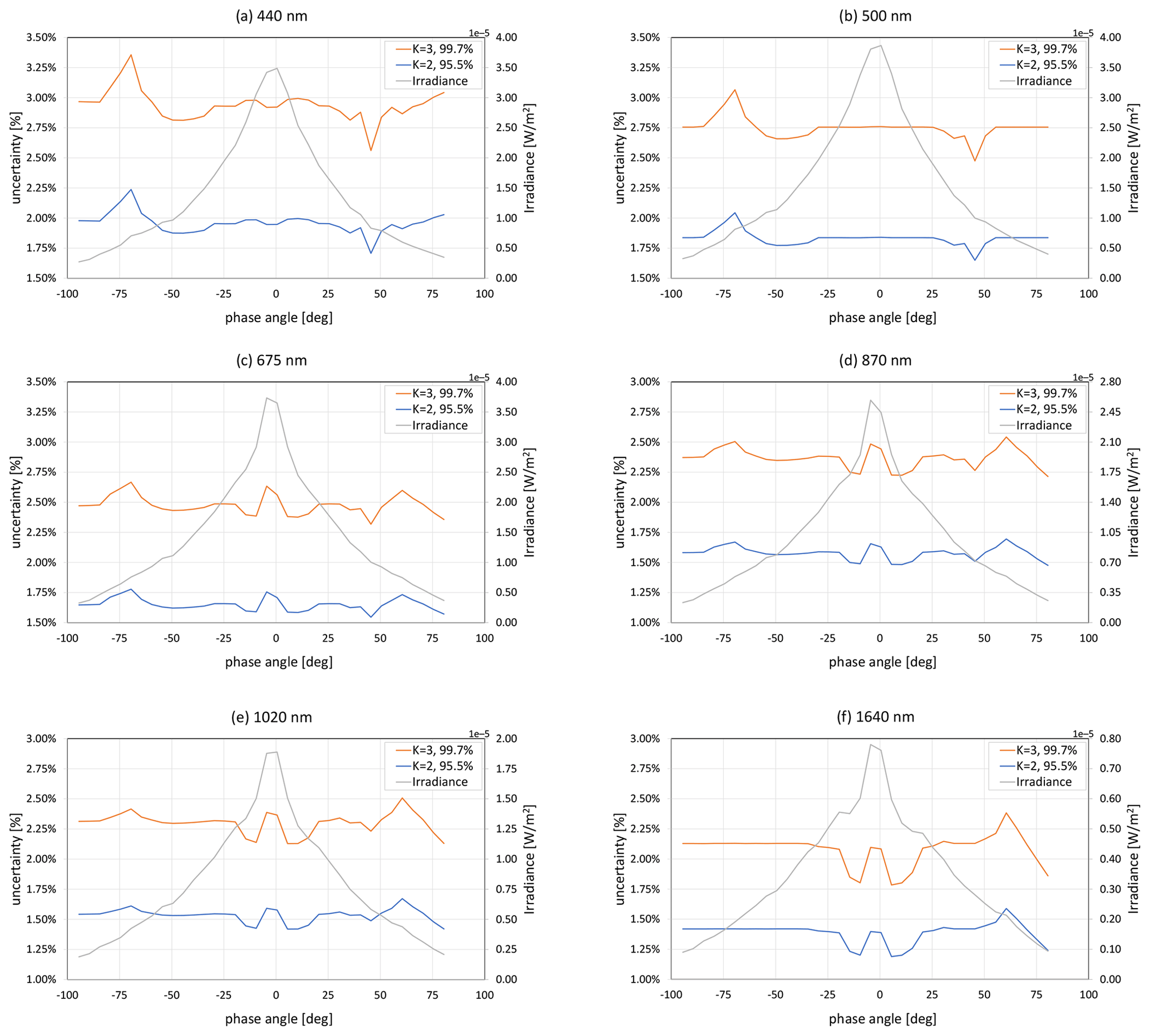
Figure 9a–f show the uncertainty levels for all bands averaged per 5° phase angle bins. Uncertainty levels at 95.5 % (k=2) and 99.7 % (k=3) confidence levels are shown, as well as the mean E_i,λ obtained over the 1000 model perturbations. At the 95.5 % confidence level all bands have uncertainties well below 2 %, except for the 440 nm band. For 99.7 % confidence, all bands have uncertainties of approximately 2.5 %, except for the 440 and 500 nm bands.

Figure 9 Uncertainty levels determined from MCUA for the Cimel photometer spectral bands.

6.4 Spectral interpolation

A reflectance spectrum of the Moon is used to increase the model spectral resolution. The lunar model calculates reflectance at the six Cimel photometer bands. The spectral range of the model spans from 440 to 1640 nm in discrete wavelength positions (Fig. 10). Therefore, in intermediate model regions, the spectrum needs to be adjusted and reconstructed.

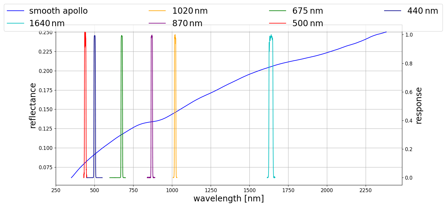
Figure 10 Cimel relative spectral response curves and interpolated smoothed lunar reflectance.

The first step is the smoothing of the measured spectrum with a reference reflectance. For the ROLO model, reflectance profiles of two Apollo 16 lunar probe samples are used to construct the reference reflectance spectrum (Kieffer and Stone, 2005). This spectrum is used to radiometrically rescale and interpolate the ROLO model output at the ROLO measurement spectral bands. The resulting reflectance R_mix,λ is a linear combination of both spectral (λ) reflectances and of R_breccia,λ and R_soil,λ measured for breccia and soil samples. For LIME, the approach used for the ROLO model is repeated.

$$\begin{array}{}\text{(17)}& R_{\mathrm{mix},\mathit{\lambda }}=\mathrm{0.05}\cdot R_{\mathrm{breccia},\mathit{\lambda }}+\mathrm{0.95}\cdot R_{\mathrm{soil},\mathit{\lambda }}\end{array}$$

The mixed reflectance is derived for every lunar model wavelength. These values are used to calculate the least absolute deviation regression values with respect to the reflectance obtained at the Cimel bands. The lunar model reflectances used in the regression are calculated for every measurement specifically. This regression results in a set of smoothing coefficients, which are applied to the spectral reflectance model, resulting in a smoothed lunar reflectance spectrum.

6.5 LIME comparisons

LIME outputs have been compared to the satellite spectral imager PROBA-V and the high-resolution (HR) Pléiades-1B. Lunar acquisitions from PROBA-V are limited in the range of lunar phase angles but cover an extensive time period. Acquisitions from Pléiades are limited in time but cover more of the lunar phase.

6.5.1 Comparison methodology

The sensor irradiance measurements E_k of the Moon at k spectral band are compared to LIME by defining the radiometric ratio between the instrument measurement (E_k,meas) and model outputs (E_k,model) with the simple relationship,

$$\begin{array}{}\text{(18)}& C_k={\displaystyle \frac{E_{k,\mathrm{meas}}}{E_{k,\mathrm{model}}}}-\mathrm{1}.\end{array}$$

LIME provides the lunar irradiance for a given viewing geometry and spectral response, and, as such, there are some limitations in the comparison which must be taken in to account. Lunar phase angles are limited to between 2 and 90°, and, at present, the model covers the spectral range of 400 to 2500 nm.

For each Earth-observation-sensor lunar acquisition, a minimum set of input parameters is given to the model for the comparison, including timestamp of acquisition (Julian Day), position of sensor (J2000 coordinates), and integrated irradiance from lunar acquisition.

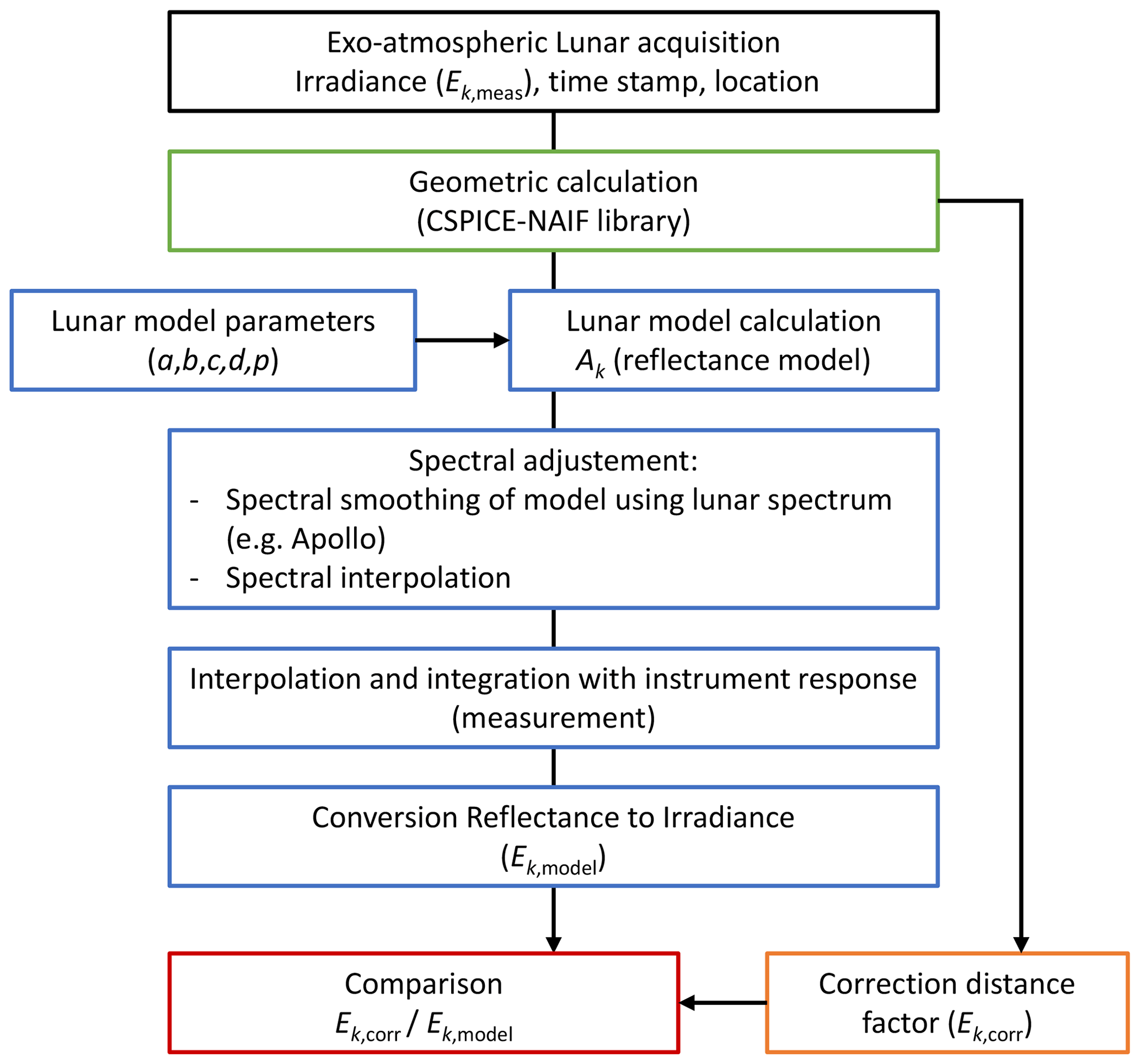
We calculate the geometric parameters per acquisition required for the comparison, i.e. phase angle; solar selenographic longitude, observer selenographic latitude and longitude; and distances between the Sun, the Moon and the observer using the NASA SPICE toolkit. LIME (interpolated using the Apollo measurements, as described in Sect. 6.4) is convolved with the normalised spectral response function of the satellite sensor to obtain the quantity E_k,model, the simulated at-sensor irradiance that can be compared with the sensor lunar measurements. Figure 11 is a flowchart of the procedure that is applied to the model input.

Figure 11 Measurement and model comparison procedure.

6.5.2 PROBA-V results

The PROBA-V instrument is a multi-spectral imager with four broad spectral bands: BLUE, RED, NIR and SWIR, centred at 450, 645, 834 and 1665 nm respectively. PROBA-V lunar images are acquired twice every month, at an approx. 7° phase angle before and after full moon. The mission has obtained images of the Moon since launch. To prepare the L1A PROBA-V data for comparison with the lunar model, several processing steps are required. Firstly, find all lunar pixels in the image (masking). Secondly, locate the centre row of the Moon and get the exact timestamp and satellite position (in J2000 coordinates) for this central row. Thirdly, convert lunar pixels into radiance (apply instrument calibration parameters). Fourthly, integrate all lunar pixels. Lastly, calculate the solid angle per pixel to finally derive lunar irradiance.

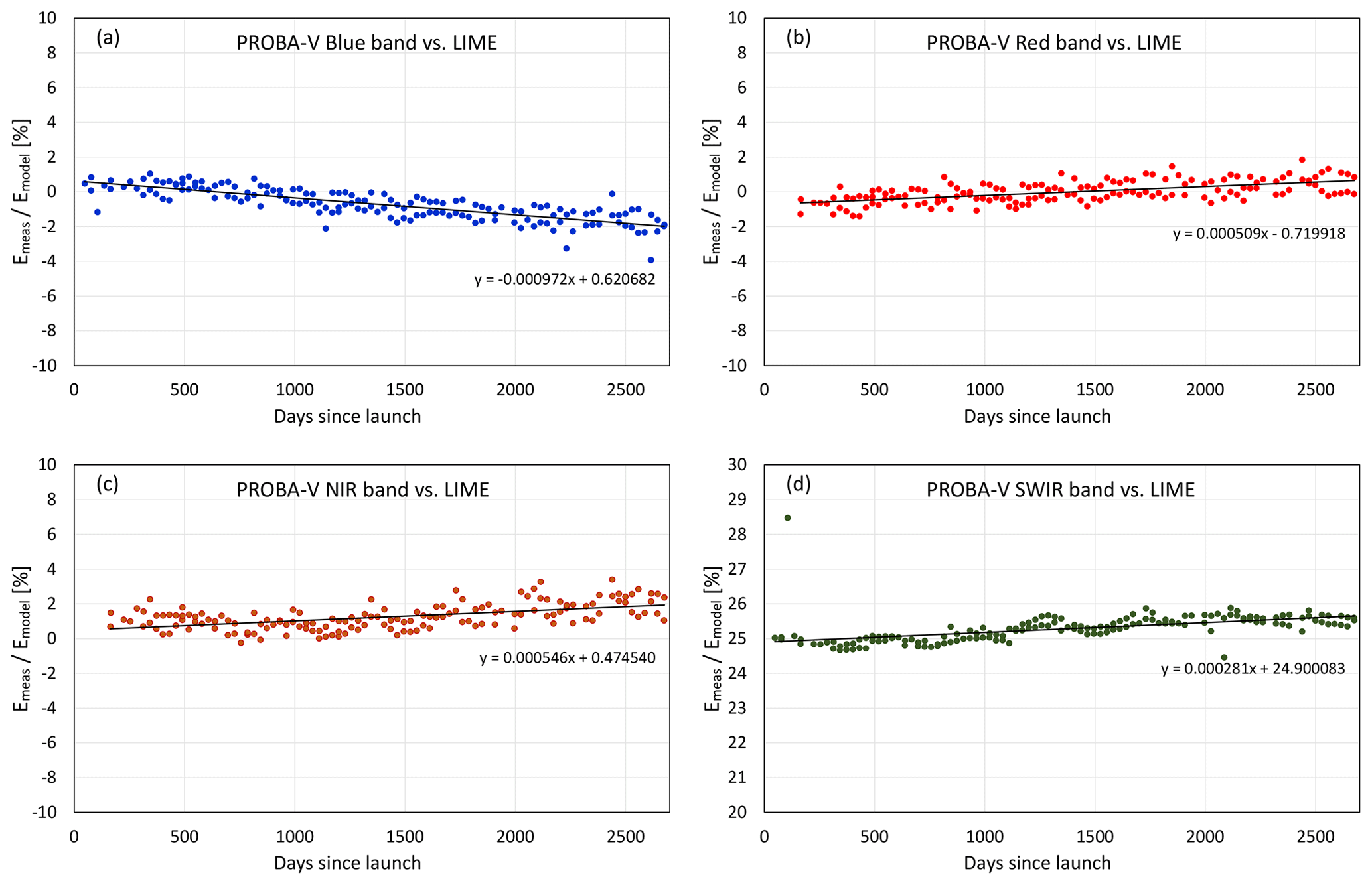
Figure 12 PROBA-V irradiance compared to LIME: differences in percent since launch of the sensor. (a) Blue band, (b) red band, (c) near-infrared (NIR) band, (d) short-wave infrared (SWIR) band.

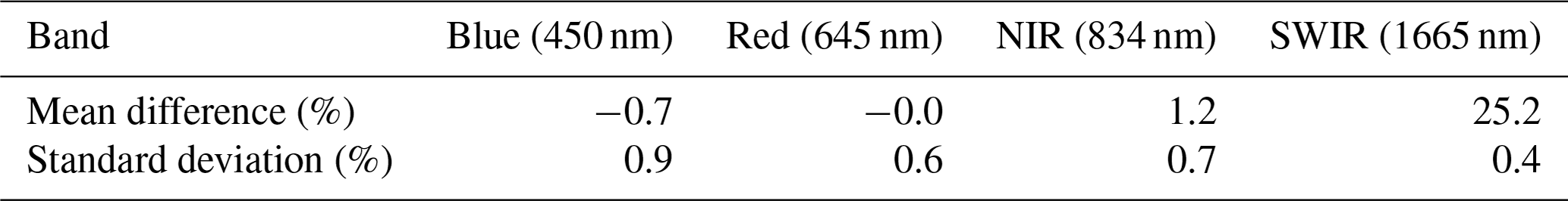
The comparisons between LIME and PROBA-V for each sensor spectral band are given in Fig. 12, with the mean differences summarised in Table 10. These comparison result in differences that are generally within ±2 %, except in the SWIR channel, where they are as high as 25 %. It is clear that the PROBA-V SWIR data need further investigation, although the most likely reason for this large difference is due to the masking process. Masking the lunar pixels is a critical step for processing and is particularly difficult for the noisier SWIR channel. Because the masking step is the basis for all further processing, the lunar irradiance values from the PROBA-V SWIR channel should be assumed to be immature.

Table 10 PROBA-V comparison to LIME: mean difference (in percent) and standard deviation for each spectral band.

A limited analysis has been done to evaluate trending capabilities of LIME. PROBA-V lunar images have previously been used to evaluate possible instrument degradation using the ROLO lunar model. As mentioned, the Moon has high reflectance and irradiance stability over time, and, consequently, yearly trends of 1 % can be detected with sensor lunar acquisitions. PROBA-V has monthly lunar data over +5 years; therefore, it is a good data set to check the trending capabilities of the lunar model. The linear regression trends for the differences between PROBA-V and LIME have been calculated (see equations in Fig. 12). These trends are cross-checked and confirmed by the application of other methods to PROBA-V sensor data, such as the desert calibration site, Libya 4 (Sterckx et al., 2014).

6.5.3 Pléiades-1B results

The Pléiades-1B HR imaging instrument (also called PHR1B) is a high-resolution multi-spectral imager. It has five spectral bands in the VNIR region: blue (430–550 nm), green (490–610 nm), red (600–720 nm), near-infrared (750–950 nm) and panchromatic (480–830 nm).

In total, 68 lunar observations are considered in this study, spanning the period between 18 February 2013 and 7 April 2017. The measurements are a combination of two campaigns in February and March 2013 recording at sparse lunar phase angles over the entire cycle. These measurements are supplemented with routine observation around a 40° phase angle acquired every few months for several years. Even if the measurements are sparse with respect to the lunar phase angle, they cover a considerably wider range of phase angles than the PROBA-V observations do.

Table 11 Pléiades-1B comparison to LIME: mean difference (in percent) and standard deviation for each spectral band.

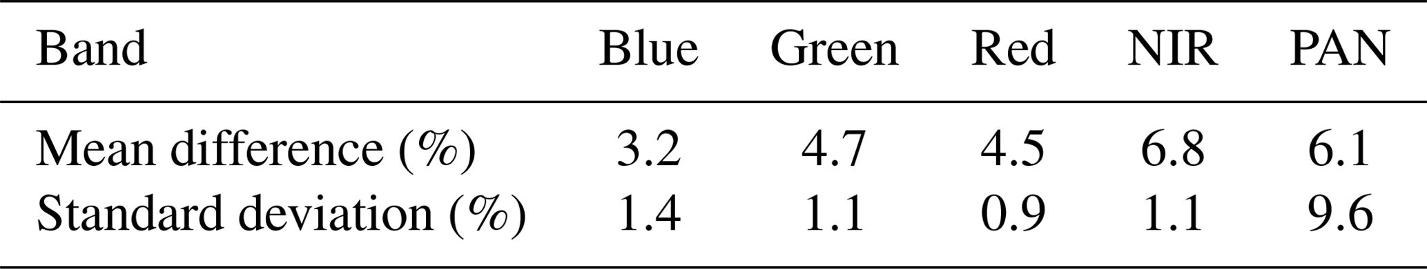
Table 12 Comparison of GIRO-ROLO to LIME computed for the PROBA-V: mean difference (in percent) and standard deviation for each spectral band.

Similarly to the PROBA-V analysis above, we have generated a model output for all Pléiades observations and spectral bands. The mean difference (in percent) has been calculated and is provided in Table 11. The output of LIME irradiance is slightly lower than the Pléiades irradiance levels, calibrated with other vicarious calibration methods. The comparison shows differences below 5 % for the visible spectral bands and above 6 % for the NIR and PAN channels.

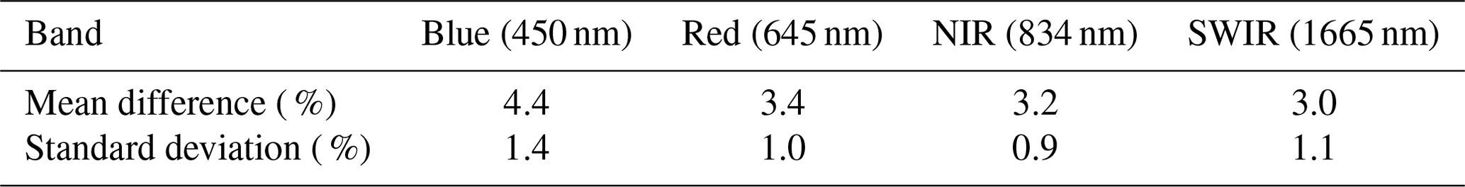
6.5.4 Comparison to GIRO

LIME has also been compared to the GSICS Implementation of the ROLO model (GIRO). The first results indicate that LIME predicts 3 %–5 % higher lunar-disc-integrated irradiance than the ROLO/GIRO model for the visible and near-infrared channels, the difference being smaller for longer wavelengths. The comparison exercise was done by simulating model outputs for the PROBA-V spectral bands. An overview of the comparison is given in Table 12.

Moreover, the LIME output was compared to Sentinel-3B measurements. The calculated instrument irradiances were within the 2 % uncertainty range for most of the bands (Neneman et al., 2020). For further details about all the mentioned comparisons, please visit https://calvalportal.ceos.org/lime-documents.

7 Conclusions and future development

A new lunar model, the Lunar Irradiance Model of ESA (LIME), has been developed. The strategy for deriving the model involved using a robust filter radiometer, the Cimel CE318, extensively used in the AERONET network, and conducting direct lunar observations at varying lunar zenith angles. These observations are suitable for deriving the top-of-atmosphere lunar irradiance using the Langley plot method, provided that the measurements are acquired at high-altitude stations such as Izaña and Teide Peak in Tenerife, Spain, where the atmospheric transmission changes minimally over the Langley period (which lasts approximately 1.5 h per night). The obtained measurements were then fitted to the ROLO equations to obtain the set of coefficients necessary for determining lunar reflectance. The lunar photometer was calibrated, ensuring that the irradiance measurements were directly traceable to the International System of Units (SI). A comprehensive uncertainty analysis was conducted, encompassing instrument calibration, individual observations and the model output. The analysis indicates that the model output uncertainty is below 2 % (k=2). When comparing the model to satellite lunar acquisitions, this estimation is generally confirmed, although further investigations are required regarding the PROBA-V SWIR channel. LIME outputs show a 3 %–5 % higher value than the GIRO-ROLO model for the visible and near-infrared channels. The performance of LIME could be further tested if employed for deriving aerosol optical depth. The lunar observations forming the basis of the current LIME span from 2018 to 2022. Additional data are still required to cover the complete range of selenographic latitude and longitude using our observation strategy. Such data are essential for establishing a comprehensive lunar irradiance model.