Seasonal characteristics of emission, distribution, and radiative effect of marine organic aerosols over the western Pacific Ocean: an investigation with a coupled regional climate aerosol model

Organic aerosols from marine sources over the western Pacific Ocean of East Asia were investigated using an online coupled regional chemistry–climate model RIEMS-Chem for the entire year 2014. Model evaluation against a wide variety of observations from research cruises and in situ measurements demonstrated a good skill of the model in simulating temporal variation and spatial distribution of particulate matter with aerodynamic diameter less than 2.5 and 10 µm (PM_2.5 and PM₁₀), black carbon (BC), organic carbon (OC), sodium, and aerosol optical depth (AOD) in the marine atmosphere. The inclusion of marine organic aerosols improved model performance on OC concentration by reducing model biases of up to 20 %. The regional and annual mean near-surface marine organic aerosol (MOA) concentration was estimated to be 0.27 µg m⁻³, with the maximum in spring and the minimum in winter, and contributed 26 % of the total organic aerosol concentration on average over the western Pacific. Marine primary organic aerosol (MPOA) accounted for the majority of marine organic aerosol (MOA) mass, and the MPOA concentration exhibited the maximum in autumn and the minimum in summer, whereas marine secondary organic aerosol (MSOA) was approximately 1–2 orders of magnitude lower than MPOA, having a distinct summer maximum and a winter minimum. MOA induced a direct radiative effect (DRE_MOA) of −0.27 W m⁻² and an indirect radiative effect (IRE_MOA) of −0.66 W m⁻² at the top of the atmosphere (TOA) in terms of annual and oceanic average over the western Pacific, with the highest seasonal mean IRE_MOA up to −0.94 W m⁻² in spring. IRE_MOA was stronger than, but in a similar magnitude to, the IRE due to sea salt aerosol on average, and it was approximately 9 % of the IRE due to anthropogenic aerosols in terms of annual mean over the western Pacific. This ratio increased to 19 % in the northern parts of the western Pacific in autumn. This study reveals an important role of MOA in perturbing cloud properties and shortwave radiation fluxes in the western Pacific of East Asia.

1 Introduction

Atmospheric aerosol is one of the most important and uncertain factors in climate change issues (IPCC, 2013). Aerosols can alter radiation balance by scattering/absorbing solar/infrared radiation and affect cloud microphysics and lifetime by activating as cloud condensation nuclei (CCN), exerting significant effects on the climate system directly and indirectly. Aerosols originated from anthropogenic and natural sources are of high spatial and temporal variability and short atmospheric lifetime relative to greenhouse gases. Consequently, aerosol radiative and climatic effects often have strong regional characteristics.

The western Pacific Ocean is frequently influenced by continental outflow of both anthropogenic and natural aerosols. Due to the continuous growth of the economy and energy consumption in the past decades, the aerosol level in China has been enhanced (Smith et al., 2011; M. Li et al., 2017) and may have potentially significant effects on radiation and cloud over not only the East Asian continent but also the wide downwind oceanic areas. Besides, East Asia is one of the major dust source regions on Earth (Shao and Dong, 2006). Dust storms often occur in spring, and dust particles can be transported eastward from the deserts and Gobi areas of northern China and southern Mongolia to the western Pacific Ocean (Gong et al., 2003), providing nutrients (e.g. iron) for phytoplankton or even triggering the outbreak of algae bloom in oceans (Calil et al., 2011; Tan et al., 2017). In addition to anthropogenic and dust aerosols, marine aerosols also significantly affect aerosol chemical composition, radiation transfer, and cloud properties in the marine atmosphere. The behaviours and climatic impacts of sea salt and non-sea-salt sulfate oxidized from dimethylsulfide (DMS) have been extensively investigated (Graf et al., 1997; Liao et al., 2004; Rap et al., 2013). In recent years, particular attention has been paid to the sources and impacts of marine organic aerosols (O'Dowd et al., 2004; Meskhidze and Nenes, 2006; Luo and Yu, 2010; Vignati et al., 2010; Gantt et al., 2011; Burrows et al., 2014; Quinn et al., 2017; Bertram et al., 2018; Huang et al., 2018); however, such studies are still very limited, especially for the western Pacific.

O'Dowd et al. (2004) found that organic matter dominated the chemical composition of marine aerosol during plankton bloom periods from spring to autumn over the North Atlantic Ocean, contributing 63 % to submicron aerosol mass. Meskhidze and Nenes (2006) revealed a significant impact of phytoplankton bloom on cloud droplet number concentration and radiation balance in the Southern Ocean and proposed a major contribution of secondary organic aerosol (SOA) from phytoplankton-produced isoprene. Some studies indicated that primary marine sources may dominate marine organic matter, whereas SOA oxidized from marine isoprene could only comprise a small fraction of the observed organic aerosol mass over marine environment (Facchini et al., 2008; Arnold et al., 2009; Myriokefalitakis et al., 2010). The estimated global emission amounts of primary marine organic matter varied largely among models. Using the global aerosol–climate model ECHAM5-HAM, Roelofs (2008) estimated a global production of marine organic aerosols to be 75 Tg C yr⁻¹. Spracklen et al. (2008) estimated the marine organic carbon emission to be approximately 8 Tg C yr⁻¹, based on the measured organic carbon mass and satellite-retrieved chlorophyll a (chl a) concentration. Vignati et al. (2010) derived a global emission of marine primary organic matter in the submicron size by the sea spray process to be 5.8 Tg C yr⁻¹, using an offline global chemistry transport model TM5, with a parameterization relating the organic emission fraction to sea surface chl a concentration. Gantt et al. (2011) found that the combination of 10 m wind speed and sea surface chl a concentration was the most consistent predictor of organic mass fraction of sea spray aerosol, based on observations from the Mace Head Atmospheric Research Station on the Atlantic coast of Ireland and a site at the Point Reyes National Seashore on the Pacific coast of California. They developed a new marine primary organic aerosol (MPOA) emission function and estimated the global annual MPOA emission associated with sea spray to be from 15.9 to 18.7 Tg C yr⁻¹ (2.8–5.6 Tg C yr⁻¹ in the submicron size). However, Quinn et al. (2014) found that the organic carbon content of sea spray aerosol is weakly correlated with the satellite-retrieved chlorophyll a concentration, based on cruise measurements in the North Atlantic Ocean and the coastal waters of California. Bates et al. (2020) reported that plankton bloom has little effect on the emission flux, organic fraction, or cloud condensation nuclei of sea spray aerosol, based on cruise experiments over the North Atlantic. Burrows et al. (2014) developed a novel physically based framework for parameterizing the organic fractionation of sea spray aerosol by consideration of ocean biogeochemistry processes, and their predicted relationships between chl a and organic fraction are similar to existing empirical parameterizations associated with ocean chl a concentrations at high chl a levels. But the empirical relationships may not be adequate to predict the organic matter (OM) fraction of sea spray aerosol outside of strong seasonal blooms.

Regarding the influence on climatic factors, such as cloud condensation nuclei (CCN), Ovadnevaite et al. (2011) revealed that MPOA was a dichotomy of low hygroscopicity and high CCN activity through an analysis of the ambient measurements of aerosol chemical compositions and size distributions at the Mace Head Atmospheric Research Station and highlighted the importance of MPOA in CCN activation over marine atmosphere. A later study of Westervelt et al. (2012) indicated that marine organic aerosols were able to increase CCN by up to 50 % in the Southern Ocean and by 3.7 % globally during the austral summer, based on the model simulation of the Goddard Institute for Space Studies Global Climate Model (GISS II-prime). Based on the measurements from seven research cruises over the Pacific, Southern, Arctic, and Atlantic oceans between 1993 and 2015, Quinn et al. (2017) indicated that sea spray aerosol generally makes a contribution of less than 30 % to CCN population at a supersaturation of 0.1 % to 1.0 % on a global basis. Burrows et al. (2022) pointed out that sea spray organic aerosol strengthened shortwave radiative cooling by clouds by −0.36 W m⁻² in the global annual mean, with the zonal mean contribution exceeding −3.5 W m⁻² in the Southern Ocean in the summertime.

The above studies reveal the important role of marine organic aerosols in chemical composition, radiation budget, and cloud microphysics, with a focus on the global scale. However, there is very limited modelling research on this important and challenging issue for the western Pacific Ocean of East Asia. To our knowledge, only two of our previous studies explored the effects of MPOA on chemical composition, radiation, cloud, and precipitation over the western Pacific in springtime with an online coupled regional chemistry–aerosol–climate model RIEMS-Chem (Han et al., 2019; Li et al., 2019), whereas the seasonality and annual aspects of MPOA and marine secondary organic aerosol (MSOA) produced by marine isoprene and terpene are still unknown. In this study, we conducted a 1-year simulation with the developed RIEMS-Chem to further explore the characteristics and radiative impacts of marine organic aerosols over the western Pacific. The model-simulated aerosol compositions were validated against a wide series of observations from ground and cruise measurements, and the simulated MSOA was evaluated by comparison with a cruise-measured secondary organic tracer in marine air masses. To our knowledge, for the first time, the seasonality of emissions, concentrations, and the direct and indirect radiative effects of marine organic aerosols have been characterized, and the annual means were estimated specifically for the western Pacific and for the key oceanic regions of concern over East Asia. This study would provide new insights into the properties and impacts of marine organic aerosols over the western Pacific and would be a necessary supplement to the global perspective of marine organic aerosols.

2 Model and data

2.1 Model description and key processes

An online coupled regional atmospheric chemistry–aerosol–climate model RIEMS-Chem was used to investigate marine organic aerosols in this study. RIEMS-Chem is composed of the host regional climate model RIEMS (Fu et al., 2005; Xiong et al., 2009; S. Y. Wang et al., 2015) and a comprehensive atmospheric chemistry–aerosol module. RIEMS was developed, based on the dynamic structure of the fifth-generation Pennsylvania State University National Center for Atmospheric Research (NCAR) Mesoscale Model (MM5; Grell et al., 1995), with a series of parameterizations to represent major physical processes, such as a modified biosphere–atmosphere transfer scheme (BATS; Dickinson et al., 1993) for land surface process; the medium-range forecasts scheme (MRF; Hong and Pan, 1996) for planetary boundary layer process; the Grell cumulus convective parameterization scheme (Grell, 1993) for convective process; the Reisner explicit moisture scheme (Reisner et al., 1998); and a modified radiation package of the NCAR Community Climate Model (CCM3; Kiehl et al., 1996) for radiation transfer processes with aerosol effect. RIEMS has participated in the Regional Climate Model Intercomparison Project (RMIP) for Asia, and it was one of the best models for predicting surface air temperature and precipitation over East Asia (Fu et al., 2005).

Atmospheric chemistry–aerosol modules have been incorporated into RIEMS in recent years, establishing the online coupled model RIEMS-Chem, which can account for the interactions among chemistry, radiation, cloud, and meteorology (Han, 2010; Han et al., 2012). RIEMS-Chem has been successfully applied in previous modelling studies on anthropogenic aerosols, mineral dust, and marine aerosols regarding spatiotemporal distributions, physical and chemical evolutions, and radiative and climatic effects over East Asia (Han et al., 2012, 2013, 2019; Li and Han, 2016a, b; Li et al., 2014, 2019, 2020). It is now participating in the international model comparison project MICS-Asia III (Model Inter-Comparison Study for Asia phase III) and shows a good ability in predicting aerosol concentrations and aerosol optical depth (AOD) over East Asia (Gao et al., 2018).

RIEMS-Chem includes atmospheric chemistry and aerosol processes, such as gas and aqueous phase chemistries, which are represented by the carbon bond (CB-IV) mechanism (Gery et al., 1989) and RADM scheme (Chang et al., 1987), respectively. Sulfate is mainly produced from the oxidation of SO₂ by the OH radical in the gas phase and the oxidation of dissolved SO₂ by H₂O₂, O₃, and metal catalysis in the aqueous phase (Chang et al., 1987). Nitrate and ammonium are produced through thermodynamic processes represented by the ISORROPIA II model (Fountoukis and Nenes, 2007). Black carbon (BC), primary organic aerosol (POA), and anthropogenic primary particulate matter (PM) are considered chemically inert. SOA formation from anthropogenic and biogenic volatile organic compound (VOC) precursors is treated by a bulk yield scheme from Lack et al. (2004), with SOA yields of 424 $\mathrm{\mu }\mathrm{g}{\mathrm{m}}^{-\mathrm{3}}{\mathrm{ppm}}^{-\mathrm{1}}$ for toluene, 342 $\mathrm{\mu }\mathrm{g}{\mathrm{m}}^{-\mathrm{3}}{\mathrm{ppm}}^{-\mathrm{1}}$ for xylene, and 762 $\mathrm{\mu }\mathrm{g}{\mathrm{m}}^{-\mathrm{3}}{\mathrm{ppm}}^{-\mathrm{1}}$ for monoterpene. For irreversible conversion of marine VOCs to SOA, a 28.6 % mass yield is assumed for isoprene (Surratt et al., 2010; Meskhidze et al., 2011) and 30 % for monoterpene (Lee et al., 2006). Heterogeneous reactions between gaseous precursors and aerosols are also taken into account (Li and Han, 2010; J. W. Li et al., 2018). Dry deposition velocity is represented by a size-dependent parameterization over different underlying surfaces (Han et al., 2004). Dry deposition velocity of particles is expressed as the inverse of the sum of resistances plus a gravitational settling term. Over sea or ocean surfaces, the quasi-laminar boundary layer (QBL) may be disrupted by bursting bubbles, resulting in an increase in the downward movement of particles, which is parameterized by the approach of Van den Berg et al. (2000), in which quasi-laminar resistance r_b is determined by Brownian diffusion and impaction when QBL is intact and by turbulence and washout velocity of particles by spray drops when QBL is broken down. Below-cloud scavenging (BCS) of particles between the cloud base and ground surface represents capture processes of particles by falling hydrometeors through Brownian and turbulent shear diffusion, interception, and inertial impaction and is parameterized by a scavenging rate, which is a function of the precipitation rate and collision efficiency of particle by the hydrometeor (Slinn, 1984).

A physically based scheme (namely the A–G scheme) developed, based on classical Köhler theory by Abdul-Razzak et al. (1998) and Abdul-Razzak and Ghan (2004), is incorporated into RIEMS-Chem to represent aerosol activation into cloud droplet processes. This scheme calculates cloud droplet number concentration (N_c) with not only the aerosol number concentration but also the aerosol size distribution and composition, updraft velocity, and ambient supersaturation. Aerosols are activated if their critical supersaturation is less than the maximum ambient supersaturation. The critical supersaturation for activating particles is determined by a curvature effect and solute effect. The maximum ambient supersaturation is calculated by solving a supersaturation balance equation (Abdul-Razzak et al., 1998). The updraft velocity is represented by the sum of the grid mean updraft velocity and subgrid updraft velocity, which is diagnosed from vertical eddy diffusivity, according to Ghan et al. (1997). The A–G scheme in RIEMS-Chem was applied over the western Pacific Ocean in spring 2014, and its prediction for hourly CCN concentration at different supersaturations has been validated by cruise measurements from the marginal seas of China to remote oceans southeast of Japan, which demonstrates a good ability, with a correlation coefficient of 0.87 and normalized mean bias within 20 %. For more details on the treatment and evaluation of marine aerosol activation, refer to Han et al. (2019). Once N_c is calculated by the A–G scheme, the cloud droplet effective radius r_e is calculated with the method of Martin et al. (1994). The activated aerosols (into cloud droplets) are removed from the air. The autoconversion rate from cloud water to rainwater is parameterized by the scheme of Beheng (1994), which depends on the N_c diagnosed and cloud liquid water content. The effect of aerosols on ice nuclei and convective cloud is not treated in this model due to limited knowledge at present.

2.2 Aerosol physical and chemical properties

In total, 10 aerosol types are simulated in RIEMS-Chem, which are sulfate (${{\mathrm{SO}}_{\mathrm{4}}}^{\mathrm{2}-}$), nitrate (${{\mathrm{NO}}_{\mathrm{3}}}^{-}$), ammonium (${{\mathrm{NH}}_{\mathrm{4}}}^{+}$), black carbon (BC), primary organic aerosol (POA), secondary organic aerosol (SOA), anthropogenic primary PM (PM_2.5 and PM₁₀), dust, and sea salt.

Based on the observational analysis of aerosol mixing state in eastern China (Ma et al., 2017; Wu et al., 2017), an internal mixing assumption is adopted for anthropogenic aerosols, and they are externally mixed with natural aerosols. The geometric mean radius and standard deviation of the anthropogenic internal mixture are estimated to be 0.11 µm and 1.65, respectively, based on field measurements (Ma et al., 2017). Mineral dust is represented by five size bins (0.1–1.0, 1.0–2.0, 2.0–4.0, 4.0–8.0, and 8.0–20.0 µm), while sea salt is represented by two size bins, with the mean fine mode radius being 0.1 µm, and the coarse mode radius being 1 µm, according to measurements from Gong et al. (1997). Feng et al. (2017) indicated that the measured total organic carbon (TOC) in the western Pacific Ocean during the same period as this study was enriched in <0.3 µm (volume median diameter), which was mainly contributed by MPOA, and the supermicron TOC was generally below the detection limit. Accordingly, the geometric mean diameter of marine organic aerosol number concentration was set to be 0.1 µm, with a standard deviation of 1.6. The number concentration is calculated by mass concentration using the formula in Curci et al. (2015). MPOA can be mixed with sea salt both externally or internally. It is more likely to be externally mixed with sea salt for finer aerosols (<200 nm in diameter) (Gantt and Meskhidze, 2013), and the effect of externally mixed MPOA was found to be much more important than that of internally mixed MPOA (Gantt et al., 2012b). So an external mixture of MPOA and sea salt is assumed in this study; this means that additional marine organic aerosols are produced to affect cloud properties and represent an upper limit of indirect effect. There is little information on the physical and chemical properties of marine organic aerosols. Some key parameters for the calculation of aerosol activation, i.e. the number of ions the salt dissociates into water, the osmotic coefficient, the mass fraction of soluble material, the density, and molecular weight are set to be 3.0, 1, 0.1, 1.5, and 90 g m⁻³, respectively, according to a few previous studies (Abdul-Razzak and Ghan, 2004; Roelofs, 2008). The soluble mass fraction of MSOA is assumed to be 0.2, which is slightly higher than that of MPOA (Liu and Wang, 2010; Westervelt et al., 2012). An OM $/$ OC ratio of 1.4 was applied to convert organic matter (OM) to organic carbon (OC) (Gantt and Meskhidze, 2013).

The hygroscopic growth of aerosol is parameterized by a κ parameterization (Petters and Kreidenweis, 2007). The hygroscopicity parameters (κ) for inorganic aerosol components, BC, POA, SOA, dust, and sea salt are set to be 0.65, 0, 0.1, 0.2, 0.01 and 0.98, respectively (Riemer et al., 2010; Liu and Wang, 2010; Westervelt et al., 2012). The hygroscopicity for MPOA and MSOA are assumed to be the same as those for anthropogenic POA and SOA. Because there was limited information on the optical properties of marine organic aerosols, the refractive index of anthropogenic POA and SOA was used instead. The aerosol refractive index and hygroscopicity (κ) of the internally mixed aerosol are calculated by the volume-weighting of the parameters for each aerosol component. Aerosol optical parameters including extinction coefficient, single scattering albedo, and the asymmetry factor are calculated by a Mie-theory-based method developed by Ghan and Zaveri (2007), in which the aerosol optical parameters are precalculated by the Mie theory and then fitted by Chebyshev polynomials, with a table of polynomial coefficients for looking up for aerosols with certain size and refractive index. For a more detailed description, refer to Li et al. (2020). This approach is much faster than the traditional Mie code, with a similar level of accuracy, and has been successfully used in estimating aerosol optical properties over East Asia (Han et al., 2011).

2.3 Anthropogenic and natural emissions

Monthly mean anthropogenic emissions of sulfur dioxide (SO₂), nitrogen (NO_x), ammonia (NH₃), non-methane volatile organic compounds (NMVOCs), carbon monoxide (CO), BC, POA, and other anthropogenic primary PM_2.5 and PM₁₀ in China for the year 2014 are obtained from the MEIC inventory (Multi-resolution Emission Inventory for China), which was developed by Tsinghua University (http://meicmodel.org.cn/, last access: 20 January 2020). Anthropogenic emissions outside China are taken from the MIX inventory, which was developed to support the Model Inter-Comparison Study for Asia phase III (MICS-Asia III) and the Hemispheric Transport of Air Pollution (HTAP) projects (M. Li et al., 2017). Both inventories of MEIC and MIX have the same resolution of 0.5°. Open biomass burning emissions of aerosols and gas precursors for the year 2014 with a spatial resolution of 0.5° are derived from the Global Fire Emissions Database, Version 4.0 (GFED4), on a daily basis (Giglio et al., 2013). The biogenic VOC emission is derived from the CAMS-BIO Global biogenic emissions dataset (CAMS-GLOB-BIO v3.1) (Granier et al., 2019; Sindelarova et al., 2014) distributed by ECCAD (Emissions of atmospheric Compounds and Compilation of Ancillary Data) GEIA (Global Emission InitiAtive) (https://permalink.aeris-data.fr/CAMS-GLOB-BIO, last access: 10 February 2020), and the monthly mean biogenic emission for the year 2014 with a horizontal resolution of 0.25° is used. All of the above emission data are bilinearly interpolated to the Lambertian projection of RIEMS-Chem. The deflation of mineral dust is represented by the scheme of Han et al. (2004), which is calculated online with RIEMS-predicted meteorology.

The generation of sea salt aerosol through bubbles is represented by Gong (2003), which is developed for a sea salt radius from 0.07 to 20 µm, based on the scheme of Monahan et al. (1986), and it is modified by considering the influences of relative humidity (RH) (Zhang et al., 2005).

Considering the strong bloom seasonality in the western Pacific region, the availability of global satellite data for chl a concentration, and the lack of cruise measurements on the relationship between sea spray organic aerosol fluxes and chl a in this region, we adopted the scheme of Gantt et al. (2011) for parameterizing marine primary organic aerosol emission in this study. The size-resolved marine primary organic aerosol (MPOA) emission is parameterized based on the method of Gantt et al. (2011, 2012a), in which the emission rate of MPOA is the product of the sea spray emission rate and organic matter fraction of sea spray aerosol, which is expressed as a function of wind speed, surface seawater chl a concentration, and aerosol size. The chl a data used in this study are the Level-3 daily mean chl a concentration (mg m⁻³) product with 9 km resolution retrieved from the VIIRS (Visible Infrared Imaging Radiometer Suite) sensor on board the Suomi National Polar-orbiting Partnership (SNPP) satellite platform (OBPG, 2022). A brief description of this scheme, together with formulas, is presented in the Supplement.

Marine isoprene emission released by phytoplankton activities is parameterized using the scheme of Gantt et al. (2009), which considers the light sensitivity of phytoplankton isoprene production and dynamic euphotic depth (see more details in the Supplement). Marine emission of monoterpene is scaled by 0.2 to those of isoprene, following the suggestion from Myriokefalitakis et al. (2010). The marine abiotic source of isoprene (due to photochemical production in the sea surface microlayer) may be important, according to recent studies (Brüggemann et al., 2018; Conte et al., 2020). This mechanism is not considered in this study because the production mechanism for marine abiotic isoprene is poorly understood at present.

2.4 Model set-up and experiment design

This study focused on the western Pacific Ocean of East Asia. The model domain covered most areas of eastern China, the Korean Peninsula, Japan, parts of Southeast Asia, and a wide area of the western Pacific Ocean (11–54° N, 89–173° E) (Fig. 1). A Lambertian conformal projection with 60 km horizontal resolution was applied in the model. There are 16 vertical layers stretched unevenly from the surface to tropopause in a terrain-following sigma coordinate, with the first eight layers within planetary boundary layer. The time step of model integration is 180 s. The simulation period was from 1 December 2013 to 31 December 2014, with the first month as model spin-up, and the whole year of 2014 was used for analysis. The year 2014 is a normal year (neither El Niño nor La Niña), which can be reflected by the El Niño–Southern Oscillation (ENSO) index (https://psl.noaa.gov/enso/mei/, last access: 15 December 2023). The reason we choose 2014 as the study period is the availability of cruise campaigns (for model validation and analysis) over the East China Sea and the western Pacific from spring to early summer, when BC and OC concentrations were measured. Final reanalysis data with 1°×1° resolution and 6 h interval from the National Centers for Environmental Prediction (NOAA/NCEP, 2000) were used to provide initial and boundary conditions for meteorology. Chemical results derived from the MOZART-4 (Model for Ozone and Related chemical Tracers, version 4; Emmons et al., 2010) simulation with 6 h interval were used to provide lateral conditions for trace gases and aerosols. The full simulation (FULL) is designed by considering all anthropogenic and natural emissions, including marine emissions of primary organic aerosol and sea salt, and a series of model simulations are also conducted to estimate the direct and indirect radiative effect of MOA and their sensitivity to MOA properties, which are described in the following sections.

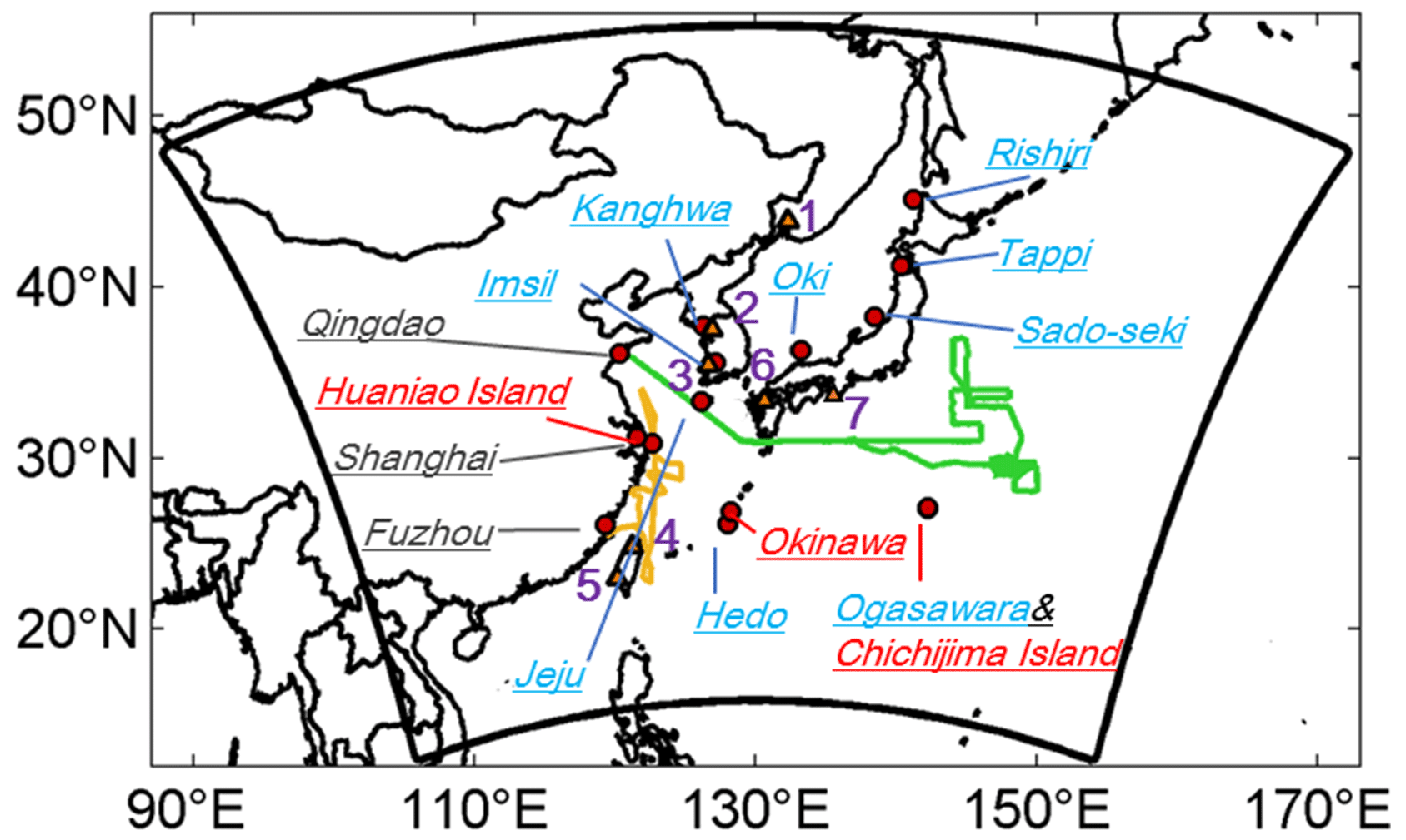
Figure 1 Model domain, observational sites, and research cruise tracks. EANET sites are marked in light blue. Observation sites of carbonaceous aerosols are marked in red (Chichijima island, Boreddy et al., 2018; Fukue Island, Kanaya et al., 2016; Okinawa Island, Kunwar and Kawamura, 2014; Huaniao island, F. W. Wang et al. (2015). Three CNEMC sites are marked in grey (Qingdao, Shanghai, and Fuzhou). Two research cruise tracks are represented by a green line (Dong Fang Hong II from 17 March to 22 April 2014; Luo et al., 2016; Feng et al., 2017) and an orange line (KEXUE 1 from 18 May to 12 June 2014; Kang et al., 2018), respectively. AERONET sites are represented by triangles with numbers (1 – Ussuriysk; 2 – Yonsei_University; 3 – Gwangju_GIST; 4 – EPA-NCU; 5 – Chen-Kung_Univ; 6 – Fukuoka; 7 – Shirahama). The written-out forms of the abbreviations are given in the text.

2.5 Observations

In situ measurements of PM₁₀, PM_2.5, and gas precursors (O₃, SO₂, and ${\mathrm{NO}}_x/{\mathrm{NO}}_{\mathrm{2}}$) at coastal and island sites in Japan and the Republic of Korea were obtained from EANET (Acid Deposition Monitoring Network in East Asia, http://www.eanet.asia, last access: 23 January 2020) (Fig. 1). Hourly concentrations of PM₁₀, SO₂, and NO_x in Japan, NO₂ in Korea, and O₃ were automatically monitored at six Japanese sites (Rishiri, Tappi, Sado-seki, Oki, Hedo, and Ogasawara) and three South Korean sites (Jeju, Kanghwa (Ganghwa), and Imsil), whereas hourly PM_2.5 concentrations were only available at three Japanese sites (Rishiri, Sado-seki, and Oki). Sodium (Na⁺) concentrations sampled on a bi-weekly basis at the six coast/island EANET sites in Japan were also collected. Besides, hourly PM₁₀ and PM_2.5 concentrations monitored in the three coastal cities of China (Qingdao, Shanghai, and Fuzhou) were also obtained from the CNEMC (China National Environmental Monitoring Centre, http://www.cnemc.cn/, last access: 23 January 2020) and used for model validation (Fig. 1).

Carbonaceous aerosol (OC and BC) concentrations measured from two research cruise campaigns covering the western Pacific during the spring and summer of 2014 (Fig. 1) were collected and used for model validation. The spring cruise campaign was carried out from 17 March to 22 April 2014 on board the research vessel (R/V) Dong Fang Hong II, which started at Qingdao, sailed to the western Pacific Ocean, and then returned (Fig. 1) (Luo et al., 2016; Feng et al., 2017). OC and BC samples were collected by an 11-stage MOUDI (Models110-IITM) (0.054–18 µm) equipped with precombusted quartz filters on board the vessel. Mass concentrations of total OC (primary and secondary) and BC were determined by the thermal/optical carbon analyser (Sunset Laboratory Inc., Forest Grove, OR). In total, 19 daily BC and OC samples were collected during the cruise. Detailed information about this campaign and the sampling and analysis techniques was documented in Feng et al. (2017). The early summer campaign was carried out from 18 May to 12 June 2014 (Kang et al., 2018). Total suspended particles (TSPs) were collected on precombusted quartz filters using a high-volume air sampler (Kimoto, Japan) on board R/V KEXUE 1 during a National Natural Science Foundation of China (NSFC) sharing cruise (Fig. 1). This campaign covered low- to mid-latitudes of the western Pacific Ocean (over the Yellow Sea and the East China Sea). In total, 51 half-day (daytime/nighttime) OC samples were obtained during this campaign. Detailed information about this campaign and samples was described in Kang et al. (2018).

Besides the in situ observations and cruise campaigns mentioned above, long-term observations of OC and BC from previous publications were collected to help model comparison and analysis. Carbonaceous aerosol samples (OC and BC) in TSPs were continuously collected on a weekly basis from 2001 to 2012 at Chichijima island (the same place as Ogasawara in Fig. 1), a remote island located in the western North Pacific. The monthly mean OC and BC concentrations of the 12-year average were reported by Boreddy et al. (2018) and used to verify the model performance over remote oceans. Measurements of seasonal mean OC and BC concentrations in TSPs at Huaniao island (a pristine island about 100 km southeast of Shanghai over the East China Sea; see Fig. 1) from October 2011 to August 2012 (F. W. Wang et al., 2015) and at Okinawa Island (the same place as Hedo in Fig. 1) in the western Pacific Ocean from October 2009 to October 2010 (Kunwar and Kawamura, 2014) were collected and used in this study. BC observations were conducted at Fukue Island west of Japan, using a continuous soot monitoring system (COSMOS) (Fig. 1) by Kanaya et al. (2016) from 2009 to 2015.

Ground observations of AOD were obtained from the Aerosol Robotic Network (AERONET, https://aeronet.gsfc.nasa.gov/, last access: 3 June 2020). Level-2 AOD observations for the year 2014 were collected at seven coastal sites shown in Fig. 1. Hourly and monthly mean observations were derived from raw data and used for model comparison and statistics calculation. AOD at 550 nm was used to match the model output. The Level-3 daily deep-blue global AOD product (in 1°×1° horizontal resolution and at 550 nm) retrieved by VIIRS sensor on board the SNPP satellite platform (Sayer et al., 2018) was also collected to examine AOD spatial distribution.

3 Model validations

In this section, the model results for OC, BC, PM₁₀, PM_2.5, sodium concentrations, and AOD were compared with a variety of observations from research cruise and monitoring networks to help evaluate the model ability over wide areas from eastern China to the western Pacific Ocean. Because the above comparison was for total OC mass concentration, we also compared the simulated SOA from marine sources to cruise measured SOA tracer to examine the model performance for marine organic aerosols. Model results are extracted from the model grid closest to the observational site for comparison with observations.

3.1 Particulate matter (PM₁₀ and PM_2.5), sodium (Na⁺), and gas precursors

As particulate matter in the remote marine atmosphere is mainly composed of sea salt, the model performance for PM₁₀ and PM_2.5 may partly reflect the model's ability to simulate sea salt, which is crucial to the estimation of MPOA emission.

Because the focus of this study is seasonal variation, the hourly PM₁₀ and PM_2.5 observations and corresponding simulations were averaged to be monthly means and shown in Fig. 2. In general, RIEMS-Chem performed quite well in simulating monthly variation in PM₁₀ concentrations at both the EANET sites (Fig. 2a–i) and CNEMC sites (Fig. 2j–l) for the year 2014, although model biases still occurred at some sites, such as the underprediction in winter and spring in Jeju (Fig. 2g) and Imsil (Fig. 2i) and the overprediction in May in Oki (Fig. 2d) and Rishiri (Fig. 2a). It was striking that the PM₁₀ concentration peaked in May and was lowest in July–August at all South Korean sites and Japanese sites over northeastern Asia (Fig. 2a–i). The long-range transport of mineral dust from north China and Mongolia in spring could contribute to the PM₁₀ maximum in May. It was noteworthy that the model-simulated seasonality and magnitude of PM₁₀ agreed quite well with observations at the four island sites of northern Japan (Rishiri, Tappi, Sado, and Oki) (Fig. 2a–d), where sea salt aerosol played a more important role than those sites in South Korea, implying that sea salt concentrations could also be well reproduced by the model. The PM₁₀ level at Ogasawara (Fig. 2f) was much lower than those at the other sites, and its seasonality was characterized by the minimum in summer (5 µg m⁻³) and the maximum in spring. The model reasonably reproduced the seasonality at Hedo (Fig. 2e) and Ogasawara (Fig. 2f) as well, although it generally predicted lower values at Hedo and higher values at Ogasawara. As for PM₁₀ concentrations at the CNEMC sites of eastern China, the model simulated PM₁₀ concentrations very well for Shanghai (Fig. 2k) and Fuzhou (Fig. 2l) in terms of both monthly variation and magnitude, showing higher values in spring and the maximum in winter in Shanghai and an almost stable level around 60 µg m⁻³ in Fuzhou throughout the year, except for the elevated value in January. The PM₁₀ level in Qingdao (Fig. 2j) was higher than those in Shanghai and Fuzhou and reached the maximum of 170 µg m⁻³ in January due to anthropogenic sources, and the peak in March resulted from the effect of mineral dust.

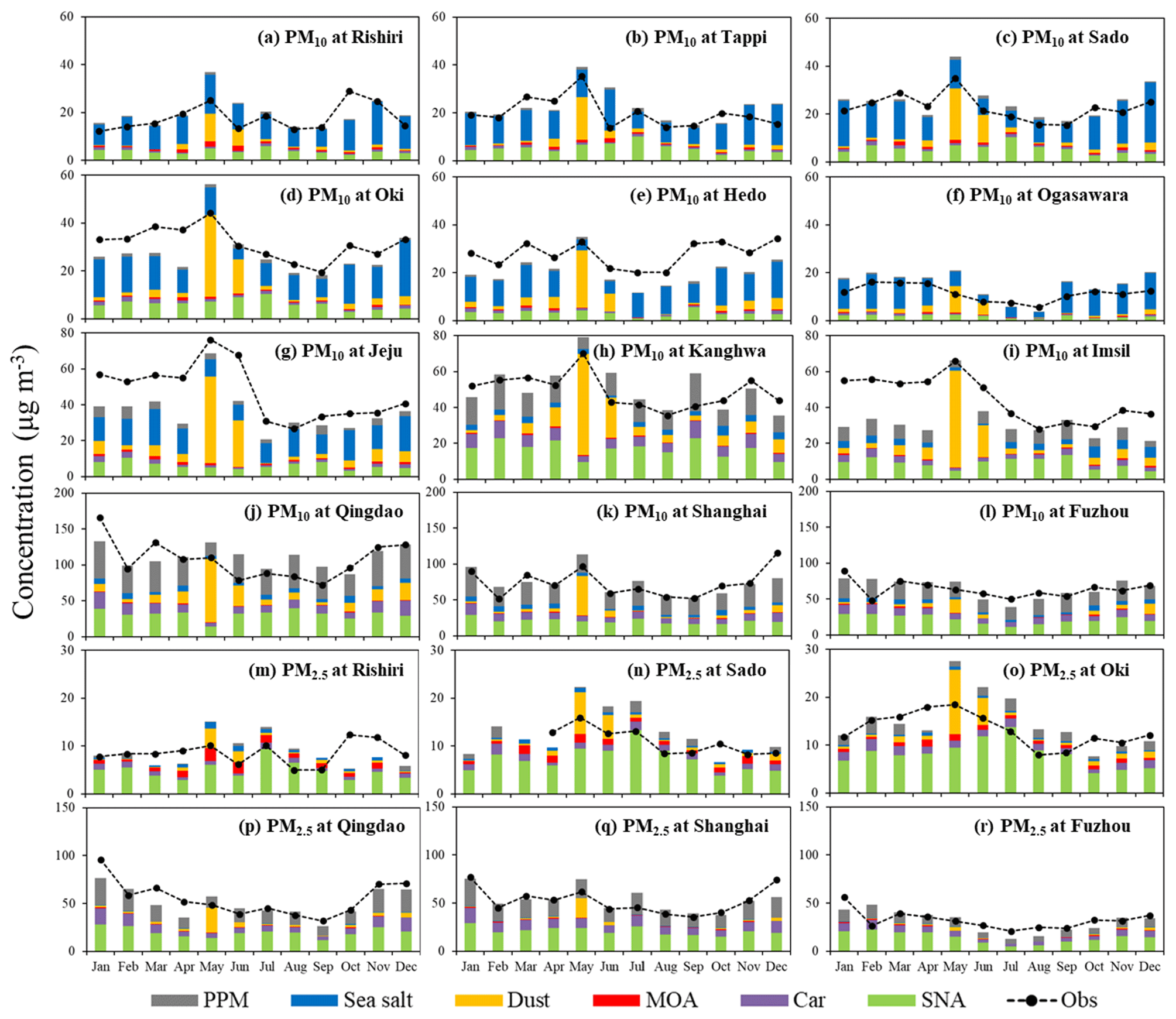
Figure 2 The model simulated (Sim) and observed (Obs) monthly PM₁₀ (a–l) and PM_2.5 (m–r) concentrations at EANET and CNEMC sites for the year 2014. The monthly data were averaged from hourly observations, and the simulations were sampled according to the observations. Simulated aerosol components (PPM is for primary anthropogenic PM; sea salt; dust; MOA; Car is for anthropogenic BC + OC; SNA is for sulfate + nitrate + ammonium) are also shown.

The monthly variations in PM_2.5 concentrations at Rishiri, Sado, and Oki (Fig. 2m–o) were similar to those of PM₁₀, but the peaks in May were not as evident as those of PM₁₀ because mineral dust comprises a small fraction of fine particles and has less effect on the PM_2.5 variation. The model reproduced PM_2.5 concentrations very well at the three coastal sites of eastern China (Fig. 2p–r), and the monthly variation in the PM_2.5 concentrations resembled those of PM₁₀ because fine particle accounts for a large fraction of PM mass in these Chinese megacities due to the dominant effect of anthropogenic sources.

Aerosol chemical components including primary anthropogenic PM, sea salt, mineral dust, MOA, anthropogenic carbonaceous aerosols (BC + OC), and inorganic aerosols (sulfate + nitrate + ammonium) in PM₁₀ and PM_2.5 at all the EANET and CNEMC sites are also shown in Fig. 2. It is found that sea salt dominated the PM₁₀ mass at the coastal and island sites of Japan and Korea in most months, except May and June when dust aerosols were abundant (Fig. 2a–g). MOA accounted for a small fraction of PM₁₀ mass at all sites, however, the relative contribution of MOA to PM_2.5 mass appeared to be larger than that of sea salt at the coastal sites of Japan (Fig. 2m–o), indicating the potential importance of MOA in fine aerosol mode in marine atmosphere.

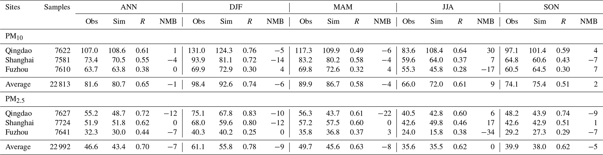
Table 1 shows that for all the nine EANET sites, the overall mean PM₁₀ concentration was 30.0 µg m⁻³ from observation and 28.5 µg m⁻³ from simulation, with the overall Pearson correlation coefficient (R) of 0.65 (0.48–0.64) and the normalized mean bias (NMB) of −5 % (−27 %–36 %). For PM_2.5, the mean concentrations averaged over the EANET sites were 10.9 µg m⁻³ from the observation and 12.3 µg m⁻³ from the simulation, with R and NMB values of 0.61 (0.53–0.64) and 12 % (0 %–21 %), respectively. The annual mean observed and simulated PM₁₀ concentrations at the three CNEMC sites (Table 2) were 81.6 and 80.7 µg m⁻³, with R and NMB values of 0.65 (0.38–0.61) and −1 % (−4 %–1 %), respectively, while the annual mean observed and simulated PM_2.5 concentrations, R, and NMB were 46.6 µg m⁻³, 43.4 µg m⁻³, 0.70​​​​​​​ (0.44–0.72), and −7 % (−12 %–0 %), respectively. The good performance statistics shown in Tables 1 and 2 suggest a good skill of RIEMS-Chem in reproducing PM levels from the coastal regions of east China to the remote western Pacific. Figure 2 and Tables 1 and 2 also illustrate that the spatial distribution of PM exhibited higher concentrations at the continental (coastal) sites (CNEMC sites, Jeju, Kanghwa, and Imsil) and lower concentrations at the remote island site (Ogasawara) over the western Pacific, which were also reasonably reproduced by RIEMS-Chem.

Table 1 Annual and seasonal performance statistics for hourly PM₁₀ and PM_2.5 concentrations (µg m⁻³) at EANET sites for the year 2014. Mean observation (Obs), mean simulation (Sim), correlation coefficient (R), and normalized mean bias (NMB in %) are listed. ANN is for annual, DJF is for December–January–February; MAM is for March–April–May; JJA is for June–July–August; and SON is for September–October–November.

Table 2 Same as Table 1 but for CNEMC sites.

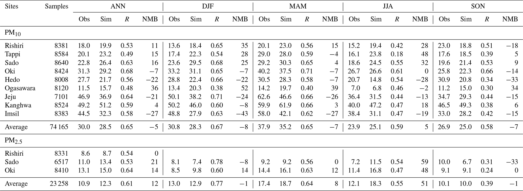
Seasonal mean statistics of PM₁₀ and PM_2.5 concentrations at the EANET and CNEMC sites were also listed in Tables 1 and 2. Statistics for spring (March, April, and May, MAM), summer (June, July, and August, JJA), autumn (September, October, and November, SON), and winter (December, January, and February, DJF) were calculated. PM₁₀ observations generally exhibited higher concentrations in MAM and DJF, moderate concentrations in SON, and lower concentrations in JJA at most sites covering coastal areas (CNEMC sites, Jeju, Kanghwa, and Imsil) and remote islands (e.g. Oki, Hedo, and Ogasawara). The model reproduced such a seasonal variation in PM₁₀ reasonably well, although some underestimations occurred from winter to spring at Jeju and Imsil (Fig. 2g and i), which could be attributed to the uncertainties in emissions (anthropogenic and biomass burning).

Comparison with observations of sodium (Na⁺) concentration at six Japanese coastal/island sites from EANET is conducted to further examine the model performance for sea salt. The modelled sodium is estimated to be 38.56 % of sea salt mass (Kelly et al., 2010), and the agreement between observation and model simulation is generally satisfactory at all sites, except at Oki in December, when the model largely underpredicts Na⁺. The model reproduces the seasonality of sodium concentration well, with the maximum in winter and the minimum in summer (Fig. 3). The model predicts sodium concentration best at Ogasawara, with the correlation coefficient of 0.85 and NMB of 5 %. The overall correlation coefficient for all sites is 0.50, with NMB of −11 % (Table S1 in the Supplement).

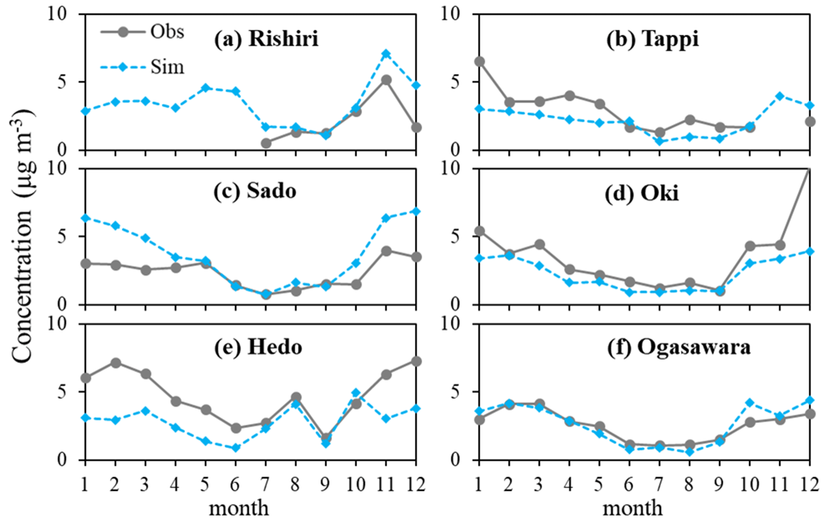
Figure 3 Observed and model simulated monthly mean sodium (Na⁺) concentrations at six coastal and island EANET sites of Japan for the year 2014.

All in all, RIEMS-Chem was able to reasonably reproduce the spatial distribution and seasonal variation in PM₁₀, PM_2.5, and sodium concentrations in the marine environment of the western Pacific. The above-mentioned good performances give us confidence in the estimation of marine sea salt emission.

In addition, the overall statistics were generally acceptable for gas precursors (O₃, SO₂, and ${\mathrm{NO}}_x/{\mathrm{NO}}_{\mathrm{2}}$), indicating atmospheric chemistry processes could be reasonably represented by the model over the western Pacific (see statistics in Table S2).

3.2 Carbonaceous aerosols

Modelled BC and OC concentrations were compared with observations from research cruises and from previous publications at coastal/remote islands. BC is considered to be inert and chemically inactive, so it is governed solely by physical processes and a good indicator of long-range transport. The analysis of BC can help identify regions with large continental influence.

3.2.1 Comparison with research cruise measurements

Figure 4a shows the observed and simulated daily BC concentrations along the cruise track during the spring campaign. An obvious spatial gradient was found for BC concentration, which was characterized by apparently higher concentrations of 0.5–4.2 µg m⁻³ over the marginal seas of China (the Yellow Sea and East China Sea for 18–19 March and 21–22 April) and very low concentrations of <0.2 µg m⁻³ over open oceans (during most of the measurement days). It is interesting to note that an observed BC peak occurred on 21 March, which could be attributed to the long-range transport of biomass burning plumes from northeastern Asia (Luo et al., 2016, 2018). The model generally reproduced the spatial and temporal variations in the BC concentration during the campaign period; however, the BC peak on 21 March was missed by the model simulation. Uncertainties in biomass burning emission could be responsible for such a model bias. On average, the measured and simulated BC concentrations during this campaign on board the Dong Fang Hong II cruise were 0.49 and 0.55 µg m⁻³, respectively, with R and NMB values of 0.87 and 13 % (Table 3).

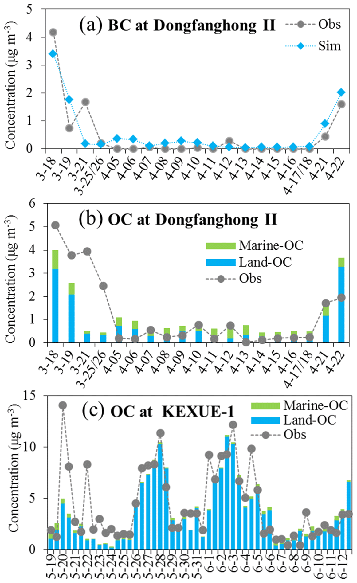
Figure 4 The model simulated (bars) and observed (dotted lines) daily BC and OC concentrations from the spring campaign (a, b) and half-day OC concentrations from the early summer campaign (c). The modelled total OC concentration was decomposed into those from marine (green bars) and land (blue bars) sources.

Table 3 Performance statistics for BC and OC from the two research campaigns in 2014. BC and OC were measured on Dong Fang Hong II during the spring campaign, whereas only OC was collected on KEXUE 1 during the early summer campaign. Mean observation (Obs), mean simulation (Sim), correlation coefficient (R), and normalized mean bias (NMB in %) are listed. The modelled concentrations of marine OC (including MPOA and MSOA) and its contribution to total OC were estimated.

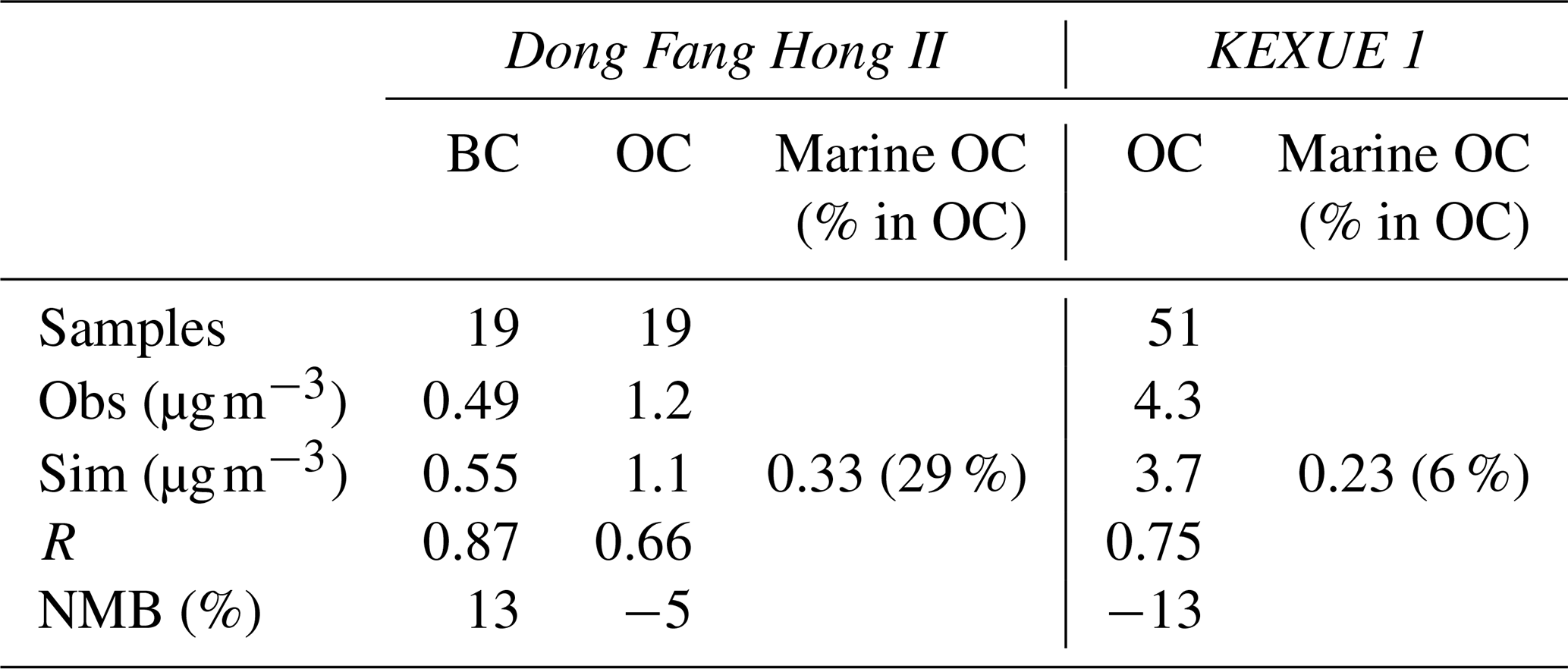
Figure 4b shows the daily mean OC concentrations from observation and model simulation for the same cruise. In general, the observed OC exhibited a similar spatial distribution and temporal variation to that of BC, with higher concentrations over the marginal seas and relatively lower concentrations over open oceans. The model generally captured the spatiotemporal features along the cruise track. Like BC, the observed OC concentrations were high on 21 and 25–26 March, mainly due to the continental outflow of biomass burning emissions from northeastern Asia, and the model largely underpredicted the high OC observation on these days. It is noteworthy that two OC peaks appeared on 10 and 12 April when the ship was over the open ocean east of Japan (the ship location was around 33.5° N, 146.0° E on 10 April and around 36.5° N, 145.0° E on 12 April, approximately 400–500 km to the east of Japan), whereas the elevation of BC concentration was not evident. Because BC and OC are often originated from the same anthropogenic and biomass sources, the inconsistency in daily variation between BC and OC in these areas implied a potential influence of marine sources rather than that from anthropogenic and biomass burning emissions. Coincidentally, during these days, daily chl a concentrations over the oceanic areas east of Japan (the region of 35 to 43° N and 140.0 to 150.0° E; north of the ship location) reached as high as 45 mg m⁻³. As a comparison, the monthly mean chl a concentration in April over the same region was in a range from 2 to 14 mg m⁻³. The apparently higher chl a concentration during these days could induce changes in marine primary organic emissions. On 10 April, the wind direction in the vicinity of the cruise was mainly southwesterly, and a backward trajectory (figure not shown) indicates that air parcels travelled over low chl a regions to the southwest of the cruise, implying a small effect of MOA. On this day, the fraction of land OC (OC originated from continental sources) in total OC was 68 %, which was larger than that of marine organic carbon (marine OC) (32 %), as shown in Fig. 4b. On 12 April, northwesterly winds prevailed over the cruise region, with backward air trajectory travelling over strong chl a regions to the northeast of Japan (figure not shown). Marine OC aerosols produced from the bloom regions could be blown to the southeast where ship located, leading to the elevation of OC concentrations (Fig. 4b). Marine OC (percentage contribution of 74 %) dominated over land OC (26 %) for the total OC concentration on this day. The model improves OC simulation on 10 and 12 April when considering marine organic aerosols (marine OC in Fig. 4b). However, it should be acknowledged that the model appears to generally overpredict OC concentrations during 5–16 April over the ocean southeast of Japan, especially on 5–6, 11, and 13 April. The high model biases could be due to potential overpredictions for either land source OC or marine source OC. The cruise campaign average OC concentration was 1.2 µg m⁻³ from the observation and 1.1 µg m⁻³ from the simulation, with R and NMB values of 0.66 and −5 %, respectively (Table 3). For the coastal/marginal sea areas (cruising time on 18 to 20 March and 20 to 22 April), the mean observed and simulated OC concentrations were 3.1 and 3.0 µg m⁻³, respectively. For open-sea areas (cruising time from 21 March to 19 April), the observed and simulated OC concentrations were 0.69 and 0.65 µg m⁻³, respectively. The inclusion of marine OC (including both primary and secondary OC) reduced the model bias from −33 % to −5 % along the cruise. The average contribution of marine OC to the total OC mass in the marine atmosphere was approximately 29 % along the cruise, with lower contributions of 11 %–27 % over the marginal seas of China (18–19 March and 21–22 April) and higher contributions of 32 %–74 % over the open oceans (5–18 April) (Fig. 4b), demonstrating an increasing importance of marine organic aerosols to total OC mass from the marginal seas to remote open oceans.

Shown in Fig. 4c is OC samples collected on board the R/V KEXUE 1 over the East China Sea during the early summer campaign and the corresponding model results along the cruise track. There were four OC peaks observed during the campaign, with three occurring over the northern parts of the East China Sea (on 20 May, 26–29 May, and 1–5 June) and one over the southern part of the East China Sea on 22 May. The model reproduced the OC variation quite well during most of the cruise track, capturing the three OC peaks over the northern parts of the East China Sea, although low biases occurred for the first peak (over the area of 27.5 to 30.0° N and 121.6 to 121.9° E). The model missed the second OC peak on 22 May over the southern part of the East China Sea (over the area of 22 to 23° N and 121.5 to 122.2° E). Kang et al. (2018) proposed that this peak was seriously affected by biogenic and biomass burning emissions from Southeast Asia (Philippines) because the OC concentrations from 21 to 25 May were characterized by a high abundance of sesquiterpene-derived SOA, which was mainly originated from terrestrial photosynthetic vegetation (e.g. trees and plants). Uncertainties in emission inventories, such as missing some biogenic sources (e.g. fungal spores; Fröhlich-Nowoisky et al., 2016) could be partly responsible for the model biases. In addition, some regions of Southeast Asia (e.g. Philippines) were not included in the study domain; instead, their influence on the study domain was represented by chemical boundary conditions from the MOZART simulation, so the uncertainties in chemical boundary conditions may also have contributed to such biases. At the time of the third (25–26° N, 118.8–121.7° E) and fourth (28–28.7° N, 119.6–122.7° E) OC peaks, the ship was close to the shore and predominately affected by continental sources (such as anthropogenic and biomass burning emissions). The model captured the peaks quite well in terms of both temporal variation and magnitude. On average, the observed and simulated OC concentrations from the KEXUE 1 cruise were 4.3 and 3.7 µg m⁻³, respectively, with R and NMB values of 0.75 % and −13 % (Table 3). The inclusion of marine OC reduced the NMB from −19 % to −13 %. Along the cruise track, marine OC was estimated to account for 6 % (1 %–60 %) of the total OC mass on average, with a lower contribution over the seas close to the continent (1 %–9 %) and a higher contribution over the seas far from the continent (7 %–60 %). During the KEXUE 1 cruise campaign, the contribution of marine OC to total OC mass was obviously lower than that during the spring campaign conducted by the Dong Fang Hong II because this cruise over the marginal seas of China was more affected by the continental outflow of anthropogenic and biomass emissions compared with that mainly over the open oceans.

3.2.2 Comparison with measurements at island and coastal sites

Figure S1 in the Supplement shows that the modelled BC is generally consistent with observations at island sites (Huaniao, Fukue, Okinawa, and Chichijima) in terms of both spatial distribution and seasonal variation, indicating a good skill of RIEMS-Chem in representing the physical processes and long-rang transport of carbonaceous aerosols over the western Pacific.

OC observations are limited in the western Pacific Ocean. We collected observations at islands from previous publications (Boreddy et al., 2018; Kunwar and Kawamura, 2014; F. W. Wang et al., 2015) for model comparison. Figure 5 shows that the model simulated and observed seasonal/monthly mean OC concentrations at the three islands. It should be kept in mind that the observations are averages of different years. At Huaniao island (Fig. 5a), a distinct seasonality of OC observation was shown, with the highest OC concentration of 4.7 µg m⁻³ in DJF, followed by 3.7 µg m⁻³ in MAM and 3.8 µg m⁻³ in SON and the minimum of 1.1 µg m⁻³ in JJA (Table 4). It was encouraging that RIEMS-Chem reproduced the OC seasonality at Huaniao island quite well (Fig. 5a), despite the different years between simulation and observation. The simulated OC was also divided into land OC and marine OC to quantify the relative contribution of these sources to total OC mass. The simulated annual mean OC concentration was 3.2 µg m⁻³, of which 2.6 µg m⁻³ (81 %) was contributed by land OC and 0.6 µg m⁻³ (19 %) by marine OC (Table 4). The simulation was very close to the observation of 3.3 µg m⁻³ (Table 4). It was striking that the inclusion of marine OC obviously improved the model performance, reducing the NMB from −21 % to −3 %, although the improvement of prediction for SOA from land source may also reduce the model bias at Huaniao island. It was noteworthy that marine OC exhibited the maximum value in MAM and the minimum value in JJA. The higher chl a concentration over the East China Sea in MAM might be responsible for the maximum at Huaniao island (Fig. 7h and Table 7), whereas the lowest sea salt emission flux could result in the minimum in summer (Table 7). In terms of seasonal mean, marine OC accounted for 12 %, 22 %, 19 %, and 23 % of the total OC concentration in DJF, MAM, JJA, and SON, respectively, with an annual mean contribution of 19 % at Huaniao island. The lowest relative contribution (12 %) of marine OC in winter was attributed to the maximum anthropogenic OC emissions in eastern China in this season.

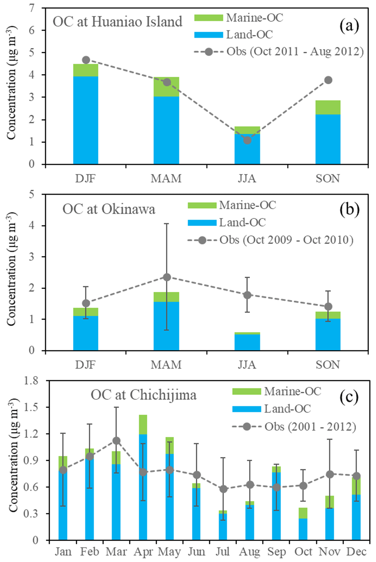
Figure 5 The model simulated (bars) and observed (dotted lines) OC concentrations at different sites. Seasonal mean concentrations were provided at (a) Huaniao island (F. W. Wang et al., 2015) and (b) Okinawa Island (Kunwar and Kawamura, 2014), while monthly mean concentrations were provided at (c) Chichijima island (Boreddy et al., 2018). Standard deviations were available at Okinawa Island and Chichijima. The modelled OC concentrations were decomposed to marine (green bars) and land (blue bars) sources. The simulation is for the year 2014.

Table 4 Comparison of model simulated and observed seasonal OC concentrations (µg m⁻³) at Huaniao island and Okinawa Island. The modelled concentrations of marine OC and its contribution to total OC were estimated. ANN is for annual; DJF is for December–January–February; MAM is for March–April–May; JJA is for June–July–August; and SON is for September–October–November.

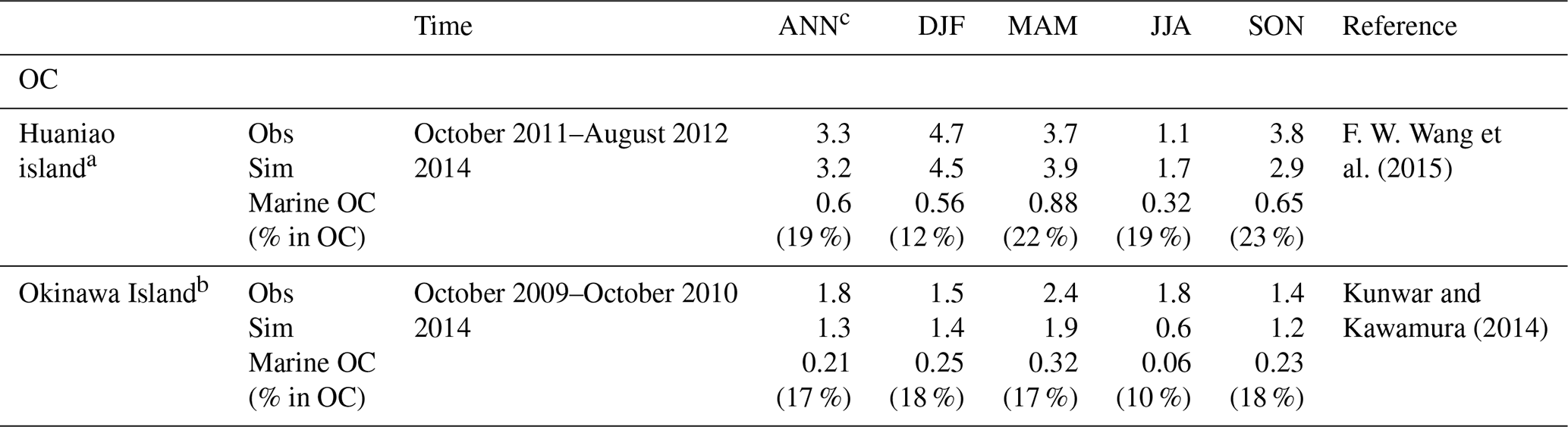
^a The location of Huaniao island is 30.86° N, 122.67° E. ^b The location of Okinawa Island is 26.15° N, 128.03° E. ^c The annual means are averages of the four seasonal means.

At Okinawa Island (Fig. 5b), the observed total OC showed the maximum in MAM, followed by that in JJA, and the lower ones in DJF and SON during October 2009–2010. Figure 5a and b also show that the seasonal cycling of the OC concentration at Okinawa Island (Fig. 5b) differed a lot from that at Huaniao island (Fig. 5a). The high OC concentration in summer at Okinawa Island could be attributed to higher SOA produced by local biogenic VOC emissions (Kunwar and Kawamura, 2014). The model generally reproduced the seasonal variation in OC, except that it predicted a lower OC level in summer, which could be due to the exclusion of local biogenic VOC emissions in the CAMS-GLOB-BIO emission inventory. In terms of annual average, the observed OC concentration was 1.8 µg m⁻³, larger than the simulations of 1.3 µg m⁻³ from the FULL case including marine OC and of 1.1 µg m⁻³ from the case excluding marine organic emissions (Table 4). The inclusion of marine organic emissions improved OC simulation at Okinawa Island, reducing the NMB from −39 % to −28 %. It was estimated that marine OC accounted for 18 %, 17 %, 10 %, and 18 % of total OC mass concentration at Okinawa Island in DJF, MAM, JJA, and SON, respectively, with an annual mean contribution of 17 %. The relatively smaller contribution of marine OC to the total OC mass at Okinawa Island than that at Huaniao island (19 %) could be attributed to the higher chl a concentration and MPOA emission flux in the marginal seas of China than those over remote western Pacific south of Japan (Fig. 7).

The long-term average (2001–2012) of monthly mean OC concentrations at Chichijima island reported by Boreddy et al. (2018) and the simulated monthly mean OC concentration in 2014 were shown in Fig. 5c. The observations show higher OC levels from January to March, mainly due to continental outflows. It was noticed that the simulated OC levels in April–May were apparently higher than observations, which could be associated with different time periods between observation and simulation and with potentially stronger continental outflows and bloom in spring 2014 than those of 10-year averages. OC observations were relatively lower in summer and autumn due to the dominance of high-pressure system and pristine ocean air mass over the western Pacific (Fig. 9d and e). The model tended to predict lower OC level in summer and autumn (Fig. 5c). Boreddy et al. (2018) indicated that in summer and autumn, OC at Chichijima was often influenced by the long-range transport of biomass burning plumes from Southeast Asia, which was not well represented in the model (using chemical boundary conditions from MOZART-4 instead) and led to low model bias. On average, the annual mean OC concentration was 0.76 µg m⁻³ from observation and 0.78 µg m⁻³ from the FULL case and 0.65 µg m⁻³ without considering marine OC (Table 5). The inclusion of marine organic emissions reduced the annual mean NMB from −13 % to 3 % and enhanced the correlation coefficient from 0.56 to 0.6 at this site. The apparently better simulation from the FULL case indicated the necessity of the inclusion of marine organic emissions for simulating OC over the remote oceans of the western Pacific. Both observation and model simulation revealed higher seasonal mean OC concentrations in MAM (observed 0.83 µg m⁻³; simulated 0.91 µg m⁻³) and DJF (observed 0.9 µg m⁻³; simulated 1.2 µg m⁻³) when the measurement site was frequently influenced by continental outflows, whereas lower concentrations in JJA (observed 0.65 µg m⁻³; simulated 0.47 µg m⁻³) and SON (observed 0.66 µg m⁻³; simulated 0.57 µg m⁻³) when clean maritime air masses or biomass burning plumes from Southeast Asia (e.g. Philippines) influenced this region. The highest marine OC concentration was 0.19 µg m⁻³ in MAM, followed by 0.16 µg m⁻³ in DJF and 0.11 µg m⁻³ in SON, and the lowest one of 0.05 µg m⁻³ in JJA. However, the percentage contribution of marine OC to the total OC mass was estimated to be largest in SON (20 %), followed by 18 % in DJF, 16 % in MAM, and the lowest in JJA (10 %), with an annual mean contribution of 16 % (Table 5). The largest contribution in SON was associated with the relatively lower total OC concentration, as shown in Fig. 5c. The relative contribution from marine OC to total OC at Chichijima island resembled that at Okinawa Island in terms of annual and season averages.

Table 5 Comparison of model simulated and observed monthly mean OC concentrations (µg m⁻³) at Chichijima island. Marine OC concentration and its contribution to total OC were estimated.

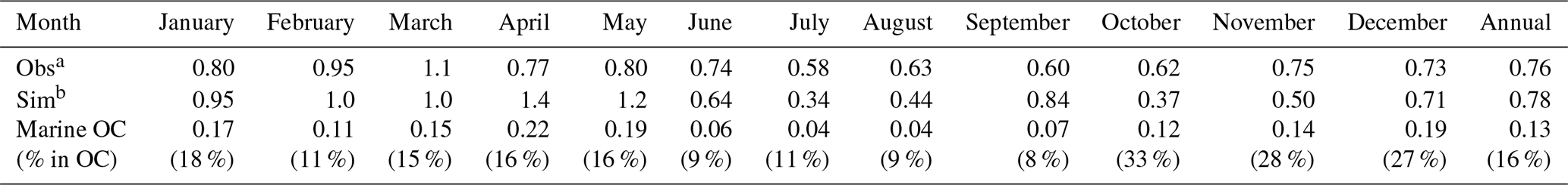
^a Observations at Chichijima island (27.07° N, 142.22° E) were obtained from Boreddy et al. (2018) and are 12-year averages (2001–2012). ^b Simulations are for the year 2014.

The above comparison, against a variety of OC observations, demonstrated the generally good skill of RIEMS-Chem in simulating OC over the western Pacific in terms of seasonal variation and magnitude. The model results from the FULL case indicated that including marine organic emissions improved OC simulation over the western Pacific Ocean.

3.2.3 SOA over the western Pacific

Recently, Guo et al. (2020) reported SOA observations in the marine atmosphere from the marginal seas of East China to the northwestern Pacific Ocean. The measurements were conducted on three research cruises in the spring and early summer of 2014 and in the spring of 2017. Total suspended particulate (TSP) samples were collected from 19 March to 21 April 2014 over the northwestern Pacific Ocean (NWPO), from 30 April to 17 May 2014 over the Yellow and Bohai seas (YBSs), and from 29 March to 4 May 2017 over the South China Sea (SCS). SOA concentration was derived using a tracer-based method. The measured SOA concentrations were 467 ± 384 ng m⁻³ over the YBSs, 617 ± 649 ng m⁻³ over the SCS, and 155 ± 236 ng m⁻³ over the NWPO, respectively. The model-simulated period and regional mean SOA concentrations were 664 ng m⁻³ over the YBSs, 466 ng m⁻³ over the SCS, and 157 ng m⁻³ over the NWPO, which were generally consistent with the above observations, although the study periods are not exactly the same. Guo et al. (2020) also present the tracer-based estimations of isoprene- and monoterpene-derived SOA in the air masses from ocean (assuming marine sources), which were 1.7 and 0.3 ng m⁻³, respectively, over the western Pacific to the southeast of Japan, whereas the modelled SOA concentrations produced from marine isoprene and monoterpene emissions along the cruise track were 1.6 and 0.28 ng m⁻³, respectively, generally agreeing with the tracer estimation. However, it should be mentioned that there could be uncertainties in such a comparison. First, the isoprene- and monoterpene-derived SOA tracers in the air masses categorized as marine sources by Guo et al. (2020) might include SOA tracers from terrestrial isoprene and monoterpene under the prevailing northwesterly winds in spring, which could bias the estimation high. Second, the measured tracer could just comprise a part of total SOA tracers, which might bias the estimation low. Despite these uncertainties, the cruise-measured SOA concentration derived from marine isoprene and monoterpene was approximately several ng m⁻³ over the western Pacific, and it can reach approximately 10 ng m⁻³, even through dividing by a mass fraction of tracer compounds to yield the concentration of total SOA tracers. It was noteworthy that both the observation and model simulation exhibited a decreasing SOA concentration from marginal seas of China to remote oceanic areas. All in all, the model reproduced the SOA levels in the marine atmosphere of the western Pacific Ocean reasonably well.

The comparison of the magnitudes between SOA and organic aerosol (OA) mass (1.4 times OC mass) concentrations shown above indicates that SOA concentration was approximately 1–2 orders of magnitude lower than OA over the western Pacific. Previous observation studies using the tracer-based approach also indicated that the percentage contribution of SOA to OA was quite low over some marine areas (Fu et al., 2011; Hu et al., 2013; Bikkina et al., 2014; Zhu et al., 2016). For example, at Okinawa Island, even when considering all biogenic sources (including isoprene, monoterpene, and sesquiterpene of both terrestrial and oceanic origins), the measured concentration of total biogenic SOA tracers was still less than 100 ng m⁻³, with majority of SOA tracers from local terrestrial biogenic emissions (Zhu et al., 2016). The above studies suggested that primary organic aerosols were more important in remote marine atmosphere.

3.3 Aerosol optical depth

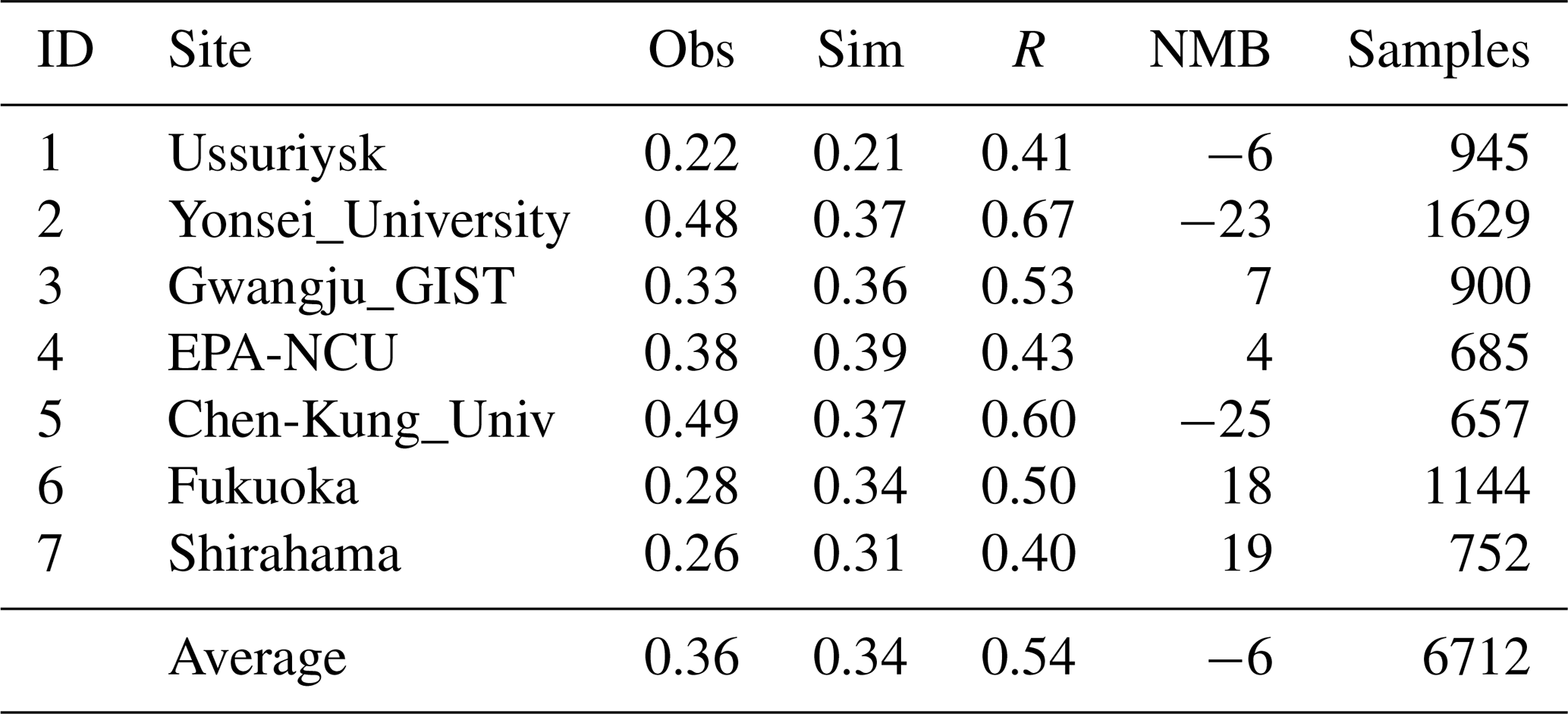
Figure 6 shows the temporal variations in the observed and simulated monthly mean AOD at the seven AERONET sites. In general, RIEMS-Chem simulated the monthly mean AOD reasonably well in terms of magnitude and monthly variation at almost all sites, although some biases occurred during some months, such as the overpredictions in August at Fukuoka and in April at the EPA-NCU (Environmental Protection Agency site at the National Central University) and the underprediction in July at Yonsei University. For the sites in the northern oceanic areas (Ussuriysk, Yonsei_University, Gwangju_GIST, and Fukuoka; Fig. 6a–d), both observations and simulations generally exhibited higher AOD values in summer (JJA), moderately high AOD values from late winter (JF) to spring (MAM), and relatively lower AOD values in autumn (SON). The simulated higher inorganic aerosol concentrations in the summer and late spring months could be responsible for the higher AOD values in these regions. Besides, the higher relative humidity in summer due to the predominant influence of maritime air masses also contributed to the maximum AOD values during summer months (JJA) at these sites. On the other hand, for the sites in the southern oceanic areas (EPA-NCU and Chen-Kung_Univ; Fig. 6e and f), the monthly mean AOD was apparently higher from March to April and remained at low levels during the remaining months. The above AOD peaks in spring could be attributed to the continental outflows of biomass burning plumes that originated from Southeast Asia, which were most active in springtime in those regions (Hsiao et al., 2017; Tao et al., 2020). Table 6 shows the performance statistics for hourly AOD at these AERONET sites. The overall annual mean AOD for the seven sites was 0.34 from model simulation, which was very close to the observation of 0.36, with the NMB of −6 % and the overall correlation coefficient of 0.54 (0.40–0.67). The statistics indicate that the model was able to reproduce aerosol optical properties over the coastal regions and islands around the western Pacific Ocean. Contributions of MOA, sea salt, and non-oceanic aerosols (anthropogenic and other natural aerosols from the Asian continent) to total AOD are also shown in Fig. 6. It clearly shows the predominant contribution to AOD from non-oceanic aerosols at all sites. It is also worth noting that AOD induced by sea salt is generally larger than that by MOA, but the values are comparable at the Chen-Kung Univ and EPA-NCU sites in spring (Fig. 6f and g).

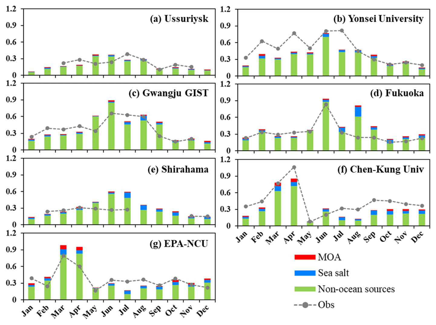
Figure 6 The model simulated (Sim) and observed (Obs) monthly mean AOD at seven AERONET sites for the year 2014. The monthly mean observations were calculated from hourly data and the simulations were sampled according to the observations. Contributions of aerosol components to total AOD by MOA, sea salt, and aerosols of non-oceanic sources (anthropogenic, dust, etc.) are shown.

Table 6 Performance statistics for hourly AOD (unitless) at AERONET sites for the year 2014. Mean observation (Obs), mean simulation (Sim), correlation coefficient (R), and normalized mean bias (NMB in %) are listed. IDs are marked in Fig. 1.

The model-simulated annual mean AOD values at 550 nm are also compared with the VIIRS retrievals (Fig. S2), which indicates the that model is generally capable of reproducing AOD distribution and magnitude in the study domain. The generally high model bias over the western Pacific could be attributed to the potential overpredictions of inorganic aerosol concentration and relative humidity. AOD reflects the column-integrated extinction coefficient due to all aerosols.

At the AERONET sites, the model-simulated annual mean percentage contribution of MOA to AOD varied from 1.4 % to 3.2 %, with an overall average of 1.9 %. For the oceanic VIIRS region, the mean contribution of MOA to AOD was approximately 2 %.

4 Model results

4.1 Marine primary organic and isoprene emissions

Figure 7 shows the estimated annual and seasonal mean MPOA emission rates over the western Pacific of East Asia. The MPOA emission mainly occurred over two hotspot regions: the marginal seas of China, including the East China Sea, the Yellow Sea, and the Bohai Sea (EYB, 27–40° N, 115–123° E; denoted in Fig. 7a), and the northern parts of the western Pacific northeast of Japan (NWP, 35–54° N, 140–160° E; denoted in Fig. 7a), with annual mean emission rates varying from $\mathrm{0.9}\times {\mathrm{10}}^{-\mathrm{2}}$ to $\mathrm{1.8}\times {\mathrm{10}}^{-\mathrm{2}}$ $\mathrm{\mu }\mathrm{g}{\mathrm{m}}^{-\mathrm{2}}{\mathrm{s}}^{-\mathrm{1}}$. In SON, high MPOA emission occurred in both the EYB and NWP regions, with the maximum up to $\mathrm{3.5}\times {\mathrm{10}}^{-\mathrm{2}}$ $\mathrm{\mu }\mathrm{g}{\mathrm{m}}^{-\mathrm{2}}{\mathrm{s}}^{-\mathrm{1}}$ in the NWP (Fig. 7e), whereas MPOA emission was very low over the EYB in JJA (Fig. 7d). The maximum seasonal mean emission rate of MPOA approached $\mathrm{3.6}\times {\mathrm{10}}^{-\mathrm{2}}$ $\mathrm{\mu }\mathrm{g}{\mathrm{m}}^{-\mathrm{2}}{\mathrm{s}}^{-\mathrm{1}}$ over the Yellow Sea in DJF (Fig. 7b), which was approximately $\mathrm{1}/\mathrm{10}$ of the annual mean anthropogenic POA emission rate in north China (on the order of 1.0–3.0 $\times {\mathrm{10}}^{-\mathrm{1}}$ $\mathrm{\mu }\mathrm{g}{\mathrm{m}}^{-\mathrm{2}}{\mathrm{s}}^{-\mathrm{1}}$). Table 7 presents the seasonal and annual averages of MPOA emission averaged over the western Pacific and the EYB and NWP regions (note that they are oceanic averages with land grids excluded). In terms of oceanic average of the western Pacific, the mean MPOA emission generally exhibited the largest emission rate in SON ($\mathrm{0.2}\times {\mathrm{10}}^{-\mathrm{2}}$ $\mathrm{\mu }\mathrm{g}{\mathrm{m}}^{-\mathrm{3}}{\mathrm{s}}^{-\mathrm{1}}$), moderately high emission rates in DJF ($\mathrm{0.18}\times {\mathrm{10}}^{-\mathrm{2}}$ $\mathrm{\mu }\mathrm{g}{\mathrm{m}}^{-\mathrm{2}}{\mathrm{s}}^{-\mathrm{1}}$) and MAM ($\mathrm{0.17}\times {\mathrm{10}}^{-\mathrm{2}}$ $\mathrm{\mu }\mathrm{g}{\mathrm{m}}^{-\mathrm{2}}{\mathrm{s}}^{-\mathrm{1}}$), and the lowest one in JJA ($\mathrm{0.08}\times {\mathrm{10}}^{-\mathrm{2}}$ $\mathrm{\mu }\mathrm{g}{\mathrm{m}}^{-\mathrm{2}}{\mathrm{s}}^{-\mathrm{1}}$), with an annual average of $\mathrm{0.16}\times {\mathrm{10}}^{-\mathrm{2}}$ $\mathrm{\mu }\mathrm{g}{\mathrm{m}}^{-\mathrm{2}}{\mathrm{s}}^{-\mathrm{1}}$ (Table 7). It is interesting to note that the seasonal variation in the MPOA emission was not consistent with that of the chl a concentration, which exhibited higher values in SON and JJA and the lowest one in DJF (Table 7). This is because the MPOA emission rate is determined by the combined effect of the chl a concentration and sea salt emission flux, and the sea salt flux is mainly controlled by surface wind speed, according to the scheme of Gong (2003). In terms of seasonal and domain average over the western Pacific, the maximum chl a concentration and the second-largest sea salt emission flux in SON led to the largest MPOA emission in autumn (Table 7). However, although the chl a concentration was also high in JJA (1.07 mg m⁻³; Table 7), the sea salt flux was minimum in JJA (0.14 $\mathrm{\mu }\mathrm{g}{\mathrm{m}}^{-\mathrm{2}}{\mathrm{s}}^{-\mathrm{1}}$, Table 7) due to the weakest wind speed (3.0 m s⁻¹; Table 9), resulting in the lowest MPOA emission in summer (Table 7). Although the sea salt emission flux reached the maximum in DJF (Table 7) due to the largest wind speed in this season (Table 9), the winter chl a concentration was lowest, leading to a moderate MPOA emission in winter (Table 7), in a similar magnitude to that in spring when moderately a high chl a concentration and relatively low sea salt flux occurred. All in all, the MPOA emission rate over the western Pacific exhibited an apparent seasonality of $\text{SON}>\text{DJF}\approx \text{MAM}>\text{JJA}$.

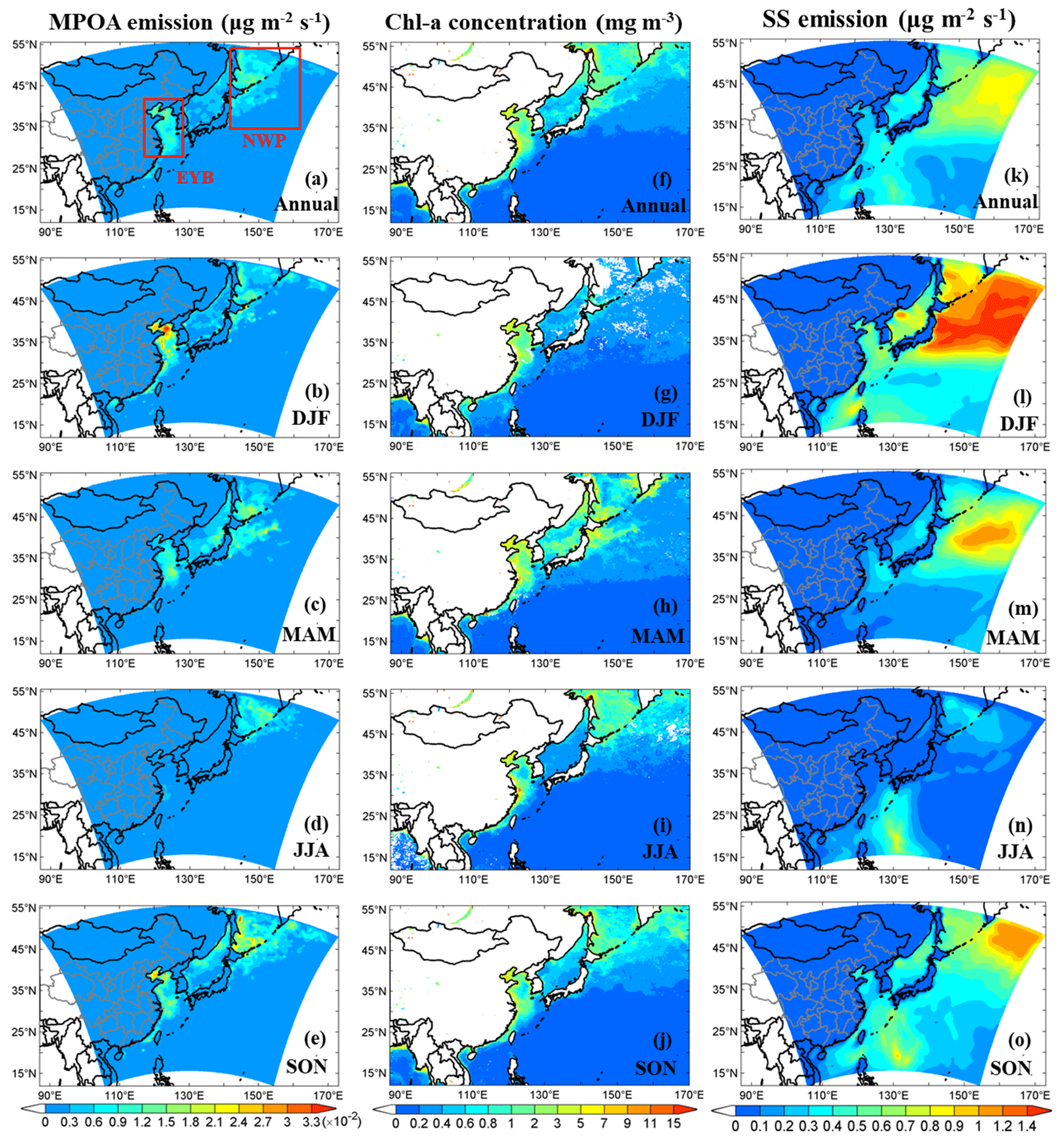
Figure 7 Model-simulated annual and seasonal mean distributions of MPOA emissions (a–e), VIIRS-retrieved surface seawater chlorophyll a (chl a) concentrations (f–j), and model-simulated sea salt (SS) emissions (k–o). Two hotspot regions are marked with red boxes, namely the region including the East China Sea, the Yellow Sea, and the Bohai Sea (EYB; 27–40° N, 115–123° E) and the region including the northern parts of the western Pacific to the northeast of Japan (NWP; 35–55° N, 140–160° E). Units are given in parentheses.

Table 7 Modelled domain and annual/seasonal mean MPOA emission rates, surface seawater chlorophyll a (chl a) concentrations, and sea salt emission fluxes over the western Pacific of East Asia (mean), the region including the East China Sea, the Yellow Sea, and the Bohai Sea (EYB) and the region including northern parts of western Pacific to the northeast of Japan (NWP).

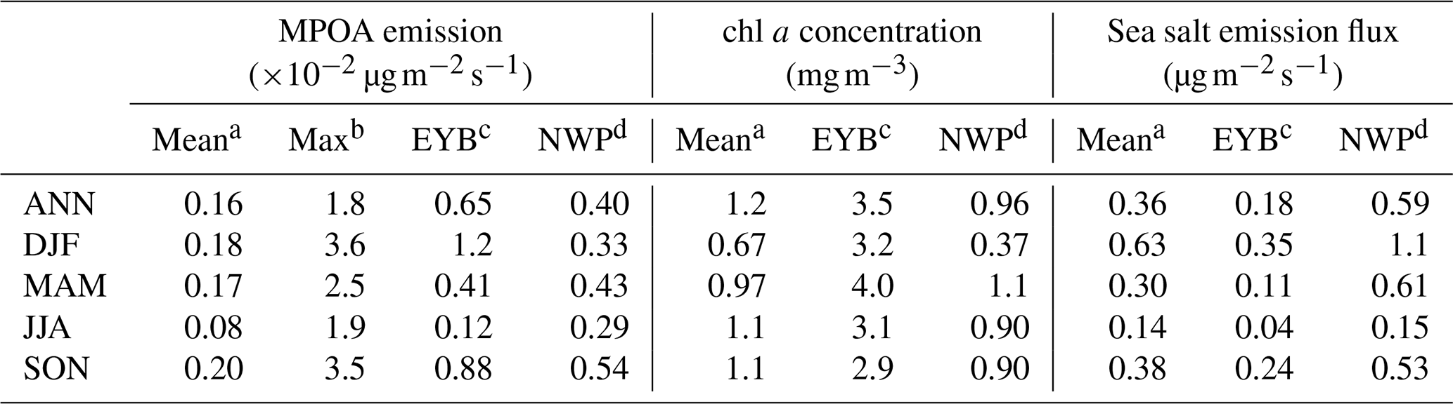
^a Mean over oceanic areas. ^b Maximum over oceanic areas. ^c Ocean areas within 27–40° N, 115–123° E. ^d Ocean areas within 35–55° N, 140–160° E.

For the EYB region, the maximum MPOA emission occurred in winter (DJF) (Fig. 7b and Table 7) with a seasonal and domain average of $\mathrm{1.2}\times {\mathrm{10}}^{-\mathrm{2}}$ $\mathrm{\mu }\mathrm{g}{\mathrm{m}}^{-\mathrm{2}}{\mathrm{s}}^{-\mathrm{1}}$, which was 10 times larger than the minimum of $\mathrm{0.12}\times {\mathrm{10}}^{-\mathrm{2}}$ $\mathrm{\mu }\mathrm{g}{\mathrm{m}}^{-\mathrm{2}}{\mathrm{s}}^{-\mathrm{1}}$ in summer (JJA) (Fig. 7d and Table 7). Although chl a concentrations were similar between DJF and JJA, the sea salt flux in DJF was approximately 9 times that in JJA (Table 7). So, the seasonality of MPOA emission in the EYB region was mainly determined by that of sea salt emission flux due to the weak seasonal variation in the chl a concentration. In contrast, in the NWP region, the MPOA emission exhibited the maximum value in SON, followed by the values in MAM and DJF, and the lowest ones in JJA (Table 7). It is interesting to note that although both the chl a concentration and sea salt emission flux were slightly higher in MAM than those in SON, the MPOA emission (related to both chl a concentration and sea salt emission) was higher in SON, which could due to the slightly negative correlation between the chl a and sea salt emission in MAM but the slightly positive one in SON. The MPOA emissions in winter and summer were at a similar level in the NWP region, which was about 40 % lower than that in autumn.

The distribution pattern of MPOA emission in the western Pacific from this study is similar to those from previous model studies (Spracklen et al., 2008; Gantt et al., 2009; Huang et al., 2018), but the magnitude of the simulated MPOA emission flux is larger than previous estimates. For example, the annual mean MPOA emission rates over the western Pacific were estimated to vary from 0.1 to approximately 12 $\mathrm{ng}{\mathrm{m}}^{-\mathrm{2}}{\mathrm{s}}^{-\mathrm{1}}$ in previous studies (Spracklen et al., 2008; Vignati et al., 2010; Gantt et al., 2011; Long et al., 2011; Huang et al., 2018), whereas the estimates in this study ranged from 3 to 18 $\mathrm{ng}{\mathrm{m}}^{-\mathrm{2}}{\mathrm{s}}^{-\mathrm{1}}$ (Fig. 7a). The larger marine POA emission estimated in this study could be attributed to the application of the daily mean chl a concentration from satellite retrievals and of a finer model grid resolution (60 km) compared with those in global models. On average, the annual MPOA emission was estimated to be 0.78 Tg yr⁻¹ over the western Pacific (with an ocean area of 1.6×10⁷ km²) from this study. The regions of EYB and NWP comprised approximately 2 % and 18 % of the western Pacific in terms of area, respectively, but they contributed 8 % and 46 % of the MPOA annual emission (Tg yr⁻¹). This study revealed that the EYB and NWP are important bloom regions, accounting for more than half of the total MPOA emission over the western Pacific.

Table S3 presents the simulated marine isoprene emission fluxes from this study and the estimates based on cruise observations over the western Pacific of East Asia from previous studies. Over the western North Pacific, the observed marine isoprene emission flux showed larger values in May (140 $\mathrm{nmol}{\mathrm{m}}^{-\mathrm{2}}{\mathrm{d}}^{-\mathrm{1}}$ from Matsunaga et al., 2002; 143.8 $\mathrm{nmol}{\mathrm{m}}^{-\mathrm{2}}{\mathrm{d}}^{-\mathrm{1}}$ from Ooki et al., 2015), a moderate value in August (55.6 $\mathrm{nmol}{\mathrm{m}}^{-\mathrm{2}}{\mathrm{d}}^{-\mathrm{1}}$ from Ooki et al., 2015), and the lowest one in winter (21.4 $\mathrm{nmol}{\mathrm{m}}^{-\mathrm{2}}{\mathrm{d}}^{-\mathrm{1}}$ from Ooki et al., 2015). The simulation from this study generally agreed with observation in terms of both seasonality and magnitude, except for the low bias in May (85–89 $\mathrm{nmol}{\mathrm{m}}^{-\mathrm{2}}{\mathrm{d}}^{-\mathrm{1}}$ vs. observation-based estimates of 140–143.8 $\mathrm{nmol}{\mathrm{m}}^{-\mathrm{2}}{\mathrm{d}}^{-\mathrm{1}}$), which could be associated with the different years. According to Eqs. (S2) and (S3) in the Supplement, both chl a concentration and incoming solar radiation determine the marine biogenic VOC emission, so the larger isoprene flux in May was mainly due to the maximum chl a concentration in spring over the NWP region (Table 7). Over the marginal seas of China, J. L. Li et al. (2017, 2018) observed higher marine isoprene emission flux in July–August (161.5 $\mathrm{nmol}{\mathrm{m}}^{-\mathrm{2}}{\mathrm{d}}^{-\mathrm{1}}$) than in October–November (48.3 $\mathrm{nmol}{\mathrm{m}}^{-\mathrm{2}}{\mathrm{d}}^{-\mathrm{1}}$) and May–June (36.1 $\mathrm{nmol}{\mathrm{m}}^{-\mathrm{2}}{\mathrm{d}}^{-\mathrm{1}}$) during 2013–2014. The model results from this study show the similar seasonal variation and magnitude of isoprene flux, with corresponding mean values of 130, 48, and 35 $\mathrm{nmol}{\mathrm{m}}^{-\mathrm{2}}{\mathrm{d}}^{-\mathrm{1}}$ during the same periods of 2014, respectively. The apparently higher isoprene flux in July–August mainly resulted from the strongest solar radiation in summer, although the chl a concentration was not highest in this season in the EYB region (Table 7). The domain-wide annual marine isoprene emission estimated over the western Pacific was 0.015 Tg yr⁻¹ in this study.

4.2 Marine organic aerosols and their relative importance

Annual and seasonal mean near-surface MOA concentrations, MSOA concentrations, and the percentage contributions of MOA to total OA mass in the study domain are shown in Fig. 8. The spatial distributions of MOA concentrations (Fig. 8a–e) generally resembled those of MPOA emissions (Fig. 7a–e). It is remarkable that the MPOA concentration (MOA minus MSOA) was approximately 1–2 orders of magnitude higher than MSOA concentration (with a concentration of several ng m⁻³) in the western Pacific (compare Fig. 8a–e vs. Fig. 8f–j), indicating that MPOA constituted a dominant fraction of MOA, which will be discussed below. Figure 8a shows that high MOA concentrations mainly occurred over the EYB and NWP regions, with the annual and regional averages being 0.48 and 0.59 µg m⁻³, respectively (Table 8), accounting for 13 % (6 %–30 %) and 42 % (30 %–60 %) of total OA mass in these two regions, respectively (Fig. 8k and Table 8). The larger MOA contribution over the NWP was attributed to the high MOA level and the relatively low total OA level there. It is worth noting that MOA even influenced the coastal areas of eastern China. The annual mean MOA concentration decreased from approximately 0.5 µg m⁻³ in coastal areas to 0.1 µg m⁻³ in the inland areas approximately 600 km away from the coastline (Fig. 8a), accounting for approximately 2 % to 6 % of the near-surface OA mass in the coastal regions (Fig. 8k). The maximum seasonal mean MOA concentration over the coastal areas of eastern China could be up to 0.6 to 0.8 µg m⁻³ in MAM (Fig. 8c) and SON (Fig. 8e). The domain and seasonal mean MOA concentration over the western Pacific exhibited the maximum value in MAM (0.37 µg m⁻³), followed by in SON (0.26 µg m⁻³), and relatively lower concentrations in JJA (0.23 µg m⁻³) and DJF (0.21 µg m⁻³) (Table 8). It is noteworthy that the seasonality of MOA concentration was different from that of the MPOA emission, which could be attributed to the influence of different meteorological conditions and physical processes. In the western Pacific, although MPOA emission peaked in SON (Table 7), the MOA concentration peaked in MAM (Table 8). It is noticed that precipitation was lowest and the wind speed was low in MAM (Fig. 9c and h; Table 9), leading to a smaller dry deposition velocity (Zhang et al., 2001) and the weakest wet scavenging, which both favoured accumulation of MOA and thus resulted in the highest MOA level in spring. On the contrary, due to the maximum wind speed and relatively more precipitation in DJF (Fig. 9b and g; Table 9), the mean MOA concentration was the lowest in winter.

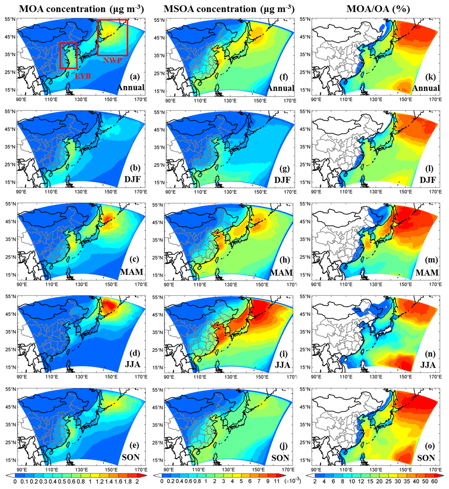
Figure 8 Model-simulated annual and seasonal mean near-surface MOA (primary + secondary) concentrations (a–e), near-surface MSOA concentrations (f–j), and percentage contributions of MOA to total OA (k–o). The two regions of the EYB (27–40° N, 115–123° E) and the NWP (35–55° N, 140–160° E) are marked in panel (a). Units are given in parentheses.

Table 8 Modelled domain and annual/seasonal mean near-surface MOA concentrations, MSOA concentrations, and MOA to total OA ratios over the western Pacific of East Asia (mean), the EYB region, and the NWP region.

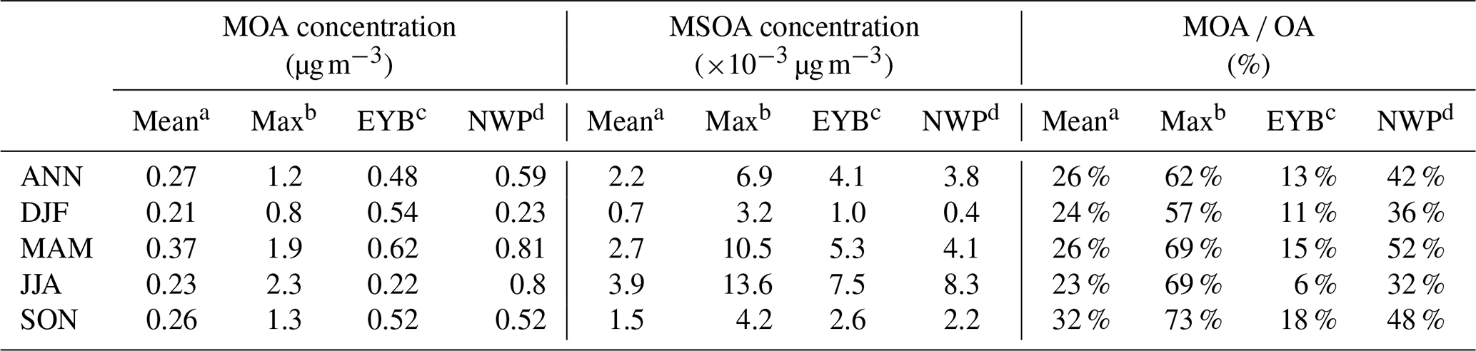
^a Mean over oceanic areas. ^b Maximum over oceanic areas. ^c Ocean areas within 27–40° N, 115–123° E. ^d Ocean areas within 35–55° N, 140–160° E.

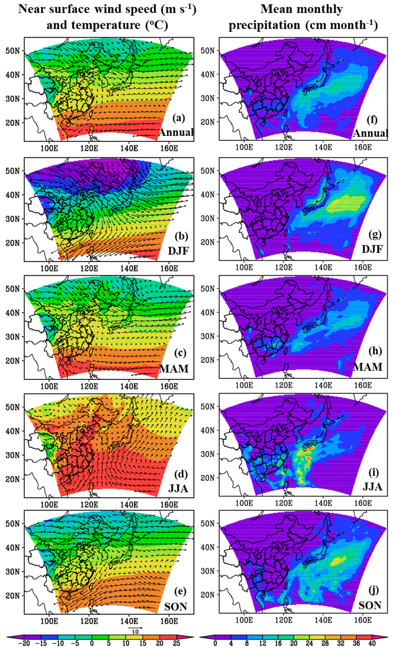
Figure 9 Model-simulated annual and seasonal mean near-surface temperatures (°C) overlaid with wind vectors (m s⁻¹) (a–e) and mean monthly precipitations (cm month⁻¹) (f–j).

Table 9 Modelled domain and annual/seasonal mean near-surface wind speed, temperature, precipitation, and relative humidity (RH) over the western Pacific of East Asia (mean), the EYB region, and the NWP region.

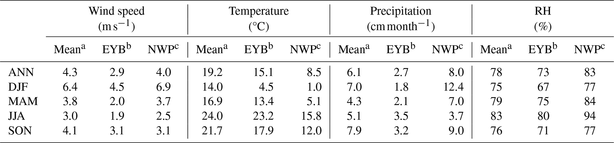
^a Mean over oceanic areas. ^b Ocean areas within 27–40° N, 115–123° E. ^c Ocean areas within 35–55° N, 140–160° E.

For the EYB region, northwesterly winds prevailed In DJF and SON and turned to northeasterly winds over marginal seas of southeastern China (Fig. 9b and e), which transported MOA from the major MPOA source region (EYB) to the northern part of the South China Sea (Fig. 8b and e). As wind speed over the EYB was low in MAM and JJA (Fig. 9c and d; Table 9), MOA was mainly restricted within this region (Fig. 8c and d). In terms of the seasonal average, the MOA concentration experienced its maximum in MAM, followed by those in DJF and SON, and the minimum in JJA (Fig. 8b–e). The seasonal and regional mean MOA concentrations over the EYB were 0.62, 0.54, 0.52, and 0.22 µg m⁻³ for MAM, DJF, SON, and JJA, respectively (Table 8). The different seasonality between MOA concentration (Table 8) and MPOA emission (Table 7) in the EYB region could also be mainly attributed to meteorological conditions. The MPOA emission was relatively low in MAM (Table 7), but the second-lowest wind speed and less precipitation (Table 9) favoured aerosol accumulation, resulting in the highest MOA concentration in spring (Table 8). The minimum MPOA emission and the maximum precipitation in JJA led to the minimum MOA concentration in summer. Although MPOA emission was largest in SON and DJF (Table 7), the maximum wind speeds (Table 9) led to the stronger dry deposition of aerosols and thus a moderate MOA concentration in the two seasons (Table 8).

MOA concentration over the NWP region exhibited apparently higher concentrations in MAM and JJA than those in SON and DJF (Fig. 8b–e), with the regional and seasonal averages reaching 0.81 µg m⁻³ in MAM, 0.80 µg m⁻³ in JJA, 0.52 µg m⁻³ in SON, and 0.23 µg m⁻³ in DJF, respectively (Table 8). Using the Goddard Earth Observing System with Chemistry (GEOS-Chem) model with a different marine organic aerosol emission scheme, Spracklen et al. (2008) also showed that in the North Atlantic, along similar latitude bands to the NWP (∼35 to ∼55° N), both observation and simulation exhibited higher OC concentrations in summer and spring than in the other seasons at the Azores islands and Mace Head. The strong seasonality of MOA over the NWP was also attributed to the combined effects of MPOA emission, wind speed, and precipitation. In MAM, the high MOA concentration over the NWP was mainly due to the large MPOA emission (Fig. 7c and Table 7), which was just smaller than that in SON, and partly due to the relatively weak dry deposition and wet scavenging caused by moderate wind speed and precipitation in this season (Table 9). In JJA, although the MPOA emission was small, the lowest wind speed and precipitation in JJA over the NWP (2.5 m s⁻¹ and 3.7 cm per grid per month; Table 9) led to the weakest dry deposition and wet scavenging of particles in summer, resulting in a long residence time of MOA and consequently the high MOA concentration in summer over the NWP. In SON, although the MPOA emission was largest over the NWP (Table 7), the mean wind speed was high over the northern part of the NWP (Fig. 9e), where MPOA emission mainly occurred (Fig. 7e), leading to strong dilution of MOA particles in autumn. Furthermore, SON had the second-largest precipitation over the NWP (Table 9), which caused strong wet scavenging of particles and also contributed to the relatively low MOA level. In DJF, the wind speed was largest, about 2 times the values in the other seasons, and the precipitation was also the maximum (Table 9; Fig. 9b and g), leading to the lowest MOA concentration in winter over the NWP (Fig. 8b and Table 8).

As shown in Fig. 8k–o, MOA generally accounted for approximately 30 % to over 60 % of total OA concentration over the remote oceans of high (>35° N) and low (<25° N) latitudes within the model domain. The large MOA $/$ OA ratios over the remote oceans of high latitude (including NWP) could be attributed to the high MOA concentration due to the large marine emissions there, whereas the large MOA $/$ OA ratios over the subtropical oceans of low latitude were mainly due to the low total OA level (small denominator). When averaged over the NWP region, the annual mean MOA $/$ OA ratio was 42 %, with higher contributions in MAM (52 %) and SON (48 %) and lower ones in DJF (36 %) and JJA (32 %) (Table 8). Although the MOA concentration over the NWP was second highest in JJA, its contribution was small because OA transported from land sources is also subject to weak dry deposition and wet scavenging, which led to a higher OA level and lower MOA $/$ OA ratio. Over the EYB region, MOA accounted for approximately 6 % to 30 % of the total OA in terms of annual mean (Fig. 8k). In terms of annual and regional average, the MOA $/$ OA ratio was 13 %, with higher ratios in SON (18 %) and MAM (15 %), a moderate one in DJF (11 %), and the lowest one in JJA (6 %) (Table 8), similar to the seasonality over the NWP. For the oceanic areas, the domain and annual mean MOA $/$ OA ratio was 26 %, indicating an important contribution of MOA to airborne OA over the western Pacific. It was found that the importance of MOA in total OA increased as the distance to the East Asian continent increased over the western Pacific. It is also interesting to note that MOA even accounted for approximately 2 %–6 % of the annual mean OA mass over portions of southeastern China (Fig. 8k), and such a contribution could be as high as 8 %–10 % in the coastal areas in SON (Fig. 8o) and MAM (Fig. 8m).

All in all, both the MOA concentration and the MOA contribution to total OA were lowest in summer (JJA) in the EYB region, which was mainly due to the much smaller MPOA emission in this season. However, in the NWP region, although the MPOA emission was also lowest in summer, the MOA concentration in summer was at a similar level to that in spring and larger than the levels in the other seasons because dry deposition velocity and precipitation were lowest in summer, which favoured aerosol accumulation and a high level of MOA.

SOA produced by marine biogenic VOCs (isoprene and terpene) was on the order of 10⁻²–10⁻³ µg m⁻³ (Fig. 8f–j), which was much lower than the MPOA concentration. The spatial distribution of MSOA exhibited high concentrations over the EYB and NWP regions in terms of annual mean, with values up to 6 ng m⁻³ (approximately 0.5 % of MOA concentration) over these two regions (Fig. 8f). MSOA concentration exhibited the maximum in JJA, with seasonal mean values of 7 to 11 ng m⁻³ extending from the marginal seas of China (EYB) to the remote western North Pacific (NWP) (Fig. 8i). MSOA distribution in MAM was similar to that in JJA but with lower mean concentrations (4–7 ng m⁻³) over the EYB and NWP regions (Fig. 8h). In SON (Fig. 8j), MSOA concentrations were 2–4 ng m⁻³ in the above two regions. In DJF (Fig. 8g), MSOA concentration was lowest, with values of 0.4–2 ng m⁻³ over the marginal seas of China and the southern parts of the model domain. The maximum seasonal mean MSOA concentration was up to 14 ng m⁻³ over the oceanic areas of the EYB to NWP regions in JJA, and the maximum daily mean MSOA value exceeded 28 ng m⁻³ on some days, e.g. 6–7 June (figure not shown). Table 8 shows the domain and seasonal/annual averages of MSOA over the oceanic regions of concern. The annual mean MSOA concentrations were 2.2, 4.1 and 3.8 ng m⁻³, averaged over the western Pacific, the EYB, and the NWP regions. It is striking that the domain average MSOA concentration consistently exhibited a distinct seasonality, with the maximum in summer and the minimum in winter throughout all the oceanic regions of the western Pacific, which resulted from the combined effects of isoprene emission flux and meteorological conditions. The domain average MSOA concentrations reached the maximum levels of 3.9, 7.5, and 8.3 ng m⁻³, respectively, over the western Pacific, the EYB, and the NWP regions in JJA. The seasonality of the MSOA concentration over the western Pacific is similar to the simulation result from Myriokefalitakis et al. (2010). According to Table 8, the annual mean fraction of MSOA in MOA was estimated to be 0.8 %, 0.9 %, and 0.6 %, over the western Pacific, the EYB, and the NWP regions, respectively. The maximum and minimum fractions of MSOA in MOA averaged over the western Pacific occurred in JJA (1.7 %) and DJF (0.3 %), respectively, with the maximum regional and seasonal average MSOA fraction up to 3.4 % in summer over the EYB region. Based on the GEOS-Chem model simulation, Arnold et al. (2009) indicated that the SOA produced by marine isoprene contributed only a very small fraction (0.01 %–1.4 %) of the observed organic aerosol mass at remote marine sites (Amsterdam Island in southern Indian Ocean, Azores islands, and Mace Head in the northern Atlantic Ocean). In a global model simulation from Myriokefalitakis et al. (2010), the annual mean marine isoprene- and monoterpene-derived SOA concentrations were approximately 0.4–1 ng m⁻³ (accounting for −0.4 % of marine OA) over the western Pacific. Meskhidze et al. (2011) illustrated that the marine SOA from phytoplankton-derived isoprene and monoterpenes contributed <10 % of surface OM concentration of marine source in most areas of the western Pacific.

4.3 Direct radiative effect due to MOA

In this section, the direct radiative effect (DRE) due to MOA (DRE_MOA) over the western Pacific of East Asia was estimated and analysed. DRE is defined as the difference in net shortwave radiation flux at the top of the atmosphere (TOA) (or at the surface) induced by aerosols. The DRE of MOA is derived by the difference between two radiation calls with aerosol optical properties (aerosol optical depth, single scattering albedo, and asymmetry factor) due to total aerosols, including sea spray (sea salt + MOA), anthropogenic aerosols, and other natural aerosols (mineral dust, SOA from vegetation emitted VOCs) in this model, and with those due to total aerosols except MOA (i.e. call twice in the radiation module in the same simulation), reflecting an instantaneous change in shortwave radiation fluxes induced by MOA. DRE of other aerosol components is estimated using the same method. The direct (indirect) radiative effect is calculated with the following general equation in this study:

$$\begin{array}{rl}{\text{D(I)RE}}_{a_i}& =(F\downarrow -F\uparrow {)}_{\mathrm{all}\mathrm{aerosols}}\\ & -(F\downarrow -F\uparrow {)}_{\text{all aerosols but }{a}_i}.\end{array}$$

Here F↓ and F↑ represent incoming and outgoing shortwave radiation fluxes, respectively, and a_i denotes a specific aerosol component, e.g. MOA.

Figure 10a–e show the annual and seasonal mean DRE_MOA at TOA under the all-sky condition. MOA induced negative DRE over the entire western Pacific. Consistent with the spatial distribution of MOA concentration, the maximum DRE_MOA up to −0.9 W m⁻² occurred over the NWP region (Fig. 10a), with statistical significance at the 99 % confidence level over limited areas of NWP (note the areas of statistical significance at the 95 % confidence level is larger). Over the EYB region, the other hotspot of the MOA mass concentration, the DRE_MOA was weaker, with an annual mean DRE_MOA of $\sim -\mathrm{0.4}$ W m⁻² (Fig. 10a). In terms of the domain average, the annual mean DRE_MOA was estimated to be −0.27 W m⁻² over the western Pacific, smaller than that over the NWP (−0.5 W m⁻²), but similar to that over the EYB (−0.33 W m⁻²) (Table 10). The weaker DRE_MOA over the EYB than over the NWP could be attributed to both the lower MOA concentration (Table 8) and lower relative humidity (73 % vs. 83 %; Table 9) because low relative humidity is unfavourable for hygroscopic growth of MOA, leading to a smaller light extinction coefficient and thus weaker DRE. The mean DRE_MOA over the western Pacific was largest in spring (−0.38 W m⁻²) and lowest in winter (−0.18 W m⁻²) (Table 10), consistent with the seasonality of MOA concentration.

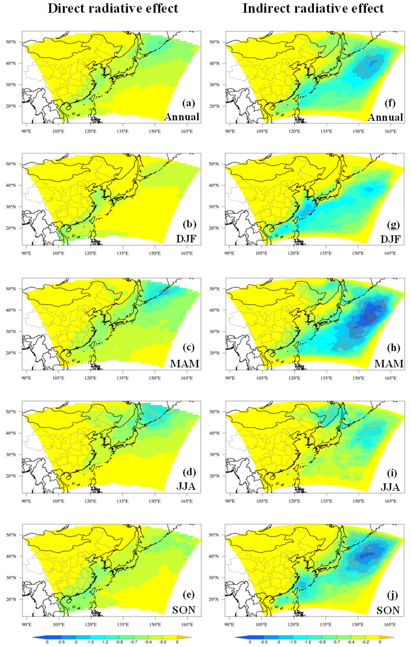
Figure 10 Model-simulated annual and seasonal mean direct radiative effect due to MOA (DRE_MOA) (a–e) and indirect radiative effect due to MOA (IRE_MOA) (f–j) at the top of atmosphere (TOA) under the all-sky condition (W m⁻²). The grey dots indicate areas where the difference is statistically significant at the 99 % confidence level, according to a two-tailed t test.

Table 10 Modelled regional and annual/seasonal mean all-sky TOA direct radiative effect (DRE) and indirect radiative effect (IRE) due to MOA, anthropogenic aerosols, and sea salt over oceanic areas of the western Pacific (WP), the EYB region, and the NWP region (W m⁻²).

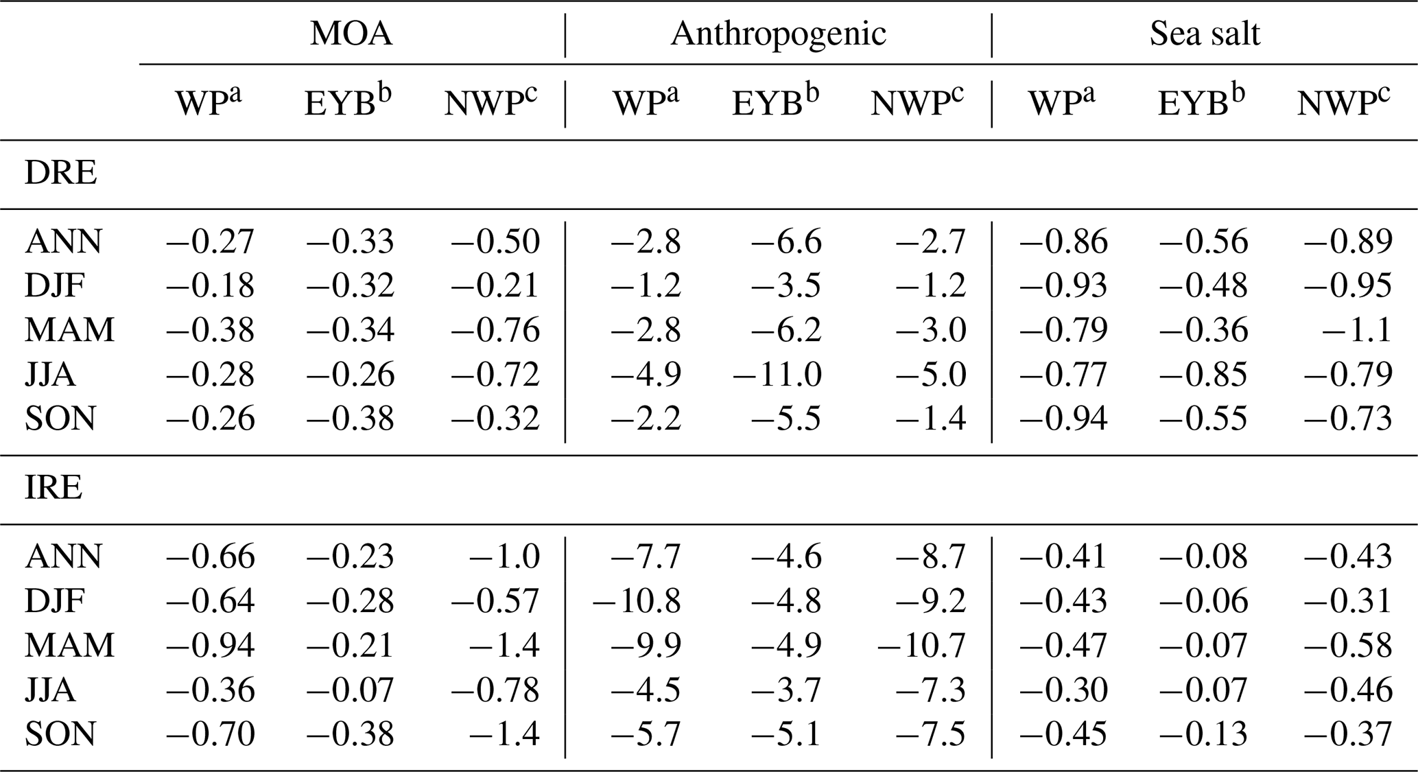
^a Mean over oceanic areas. ^b 27–40° N, 115–123° E. ^c 35–55° N, 140–160° E.

In the NWP region, MOA induced the largest DRE up to −2.0 W m⁻² to the northeast of Japan in MAM (Fig. 10c), followed by that in JJA (up to −1.5 W m⁻²) (Fig. 10d), with statistical significance at the 99 % confidence level, mainly due to higher MOA concentrations in the two seasons. The DRE_MOA value was relatively low in SON ($\sim -$0.7 W m⁻²) (Fig. 10e), and it was lowest in DJF, with the maximum of just −0.4 W m⁻² without statistical significance (Fig. 10b) due to the lowest MOA concentration in winter (Table 8). The regional and seasonal means of DRE_MOA over the NWP were estimated to be −0.76, −0.72, −0.32, and −0.21 W m⁻² in MAM, JJA, SON, and DJF, respectively (Table 10). On the contrary, in the EYB region, DRE_MOA exhibited a different seasonal trend from that over the NWP, exhibiting the largest DRE in SON (Fig. 10e), moderate DREs in MAM (Fig. 10c) and DJF (Fig. 10b), and the lowest one in JJA (Fig. 10d), with corresponding mean values of −0.38, −0.34, −0.32, and −0.26 W m⁻², respectively, for the four seasons (Table 10). The different seasonal variation in DRE in EYB and NWP could be mainly attributed to the different seasonality of MOA concentrations in these two regions.

It is of interest to estimate the relative importance of MOA in directly perturbing solar radiation compared with other types of aerosols over the western Pacific. Table 10 lists the simulated annual and seasonal mean DREs due to sea salt and anthropogenic aerosols over the western Pacific and the regions of NWP and EYB, respectively. It is noted that the annual mean DRE_MOA was approximately one-third of that due to sea salt and 1 order of magnitude lower than that due to anthropogenic aerosols on average over the western Pacific in this simulation. Over the EYB region, DRE_MOA was almost negligible compared to that by anthropogenic aerosols due to the predominance of anthropogenic emissions near the continent; however, it is noteworthy that DRE_MOA was comparable in magnitude to the DRE by sea salt, especially in springtime (−0.34 W m⁻² vs. −0.36 W m⁻² in MAM) when the MOA concentration reached its maximum (Table 8). Over the remote oceans (NWP), DRE_MOA was approximately 19 % of the DRE by anthropogenic aerosols due to weakened influence of continental anthropogenic emissions over open oceans, and it was comparable in magnitude to the DRE by sea salt, especially in summertime (0.72 W m⁻² vs. 0.79 W m⁻²) when sea salt emission flux was lowest (Table 7). The annual and regional mean all-sky DRE_MOA values were approximately 10 %, 5 %, and 19 % of the DREs due to anthropogenic aerosols over the western Pacific, the EYB, and the NWP, respectively, and it was comparable in magnitude to the DREs by sea salt in the EYB and NWP regions.

It should be mentioned that due to the much smaller MSOA concentration compared to the MPOA concentration, the above DRE_MOA was dominantly contributed by MPOA, similar to the findings from previous studies (Arnold et al., 2009; Booge et al., 2016; Li et al., 2019). MPOA also dominated over MSOA in the following IRE estimation.

4.4 Indirect radiative effect due to MOA

The first indirect effect refers to that aerosol particles tend to increase cloud droplet number concentration, decrease cloud effective radius under stable cloud liquid water content, and thus modify cloud optical properties and radiation, which is also denoted as the indirect radiative effect (IRE) in this study. IRE due to marine organic aerosols (IRE_MOA) over the western Pacific of East Asia was explored in this section. The model is able to generally reproduce the major distribution features of annual mean cloud fraction and cloud optical depth in comparison with MODIS retrievals, which generally shows higher values from southeastern China to the NWP region (figure not shown). The first indirect radiative effect or IRE of MOA is estimated by the instantaneous difference in net shortwave radiation flux at TOA (or at the surface) between two radiation calls with cloud properties (cloud optical depth, cloud single scattering albedo, and cloud asymmetry factor) due to total aerosols and with those due to total aerosols except MOA in one simulation. The lower bound of the cloud droplet number concentration (N_c) is set to 10 cm⁻³, which roughly represents N_c in liquid clouds in clean ocean conditions, according to satellite observations and global simulations. Hoose et al. (2009) pointed out that the choice of the low bound of N_c may lead to uncertainties in the IRE estimation.

Here, the calculation of IRE due to MOA (the sum of MPOA and MSOA) is called the base case (BASE), from which a series of sensitivity simulations are carried out below.

N_c, due to aerosol activation, is diagnosed by the A–G scheme, then the cloud effective radius r_e is calculated as a function of N_c and cloud liquid water content, following the approach of Martin et al. (1994), and the cloud optical parameters (liquid cloud extinction optical depth, single scatter albedo, asymmetry factor, etc.) are calculated by the scheme of Slingo (1989). Finally, shortwave radiation fluxes are calculated by the CCM3 radiation scheme (Kiehl et al., 1996).

The annual and seasonal mean IRE_MOA values at TOA are shown in Fig. 10f–j. IRE_MOA was negative in the entire domain, resulting from a series of changes in cloud properties induced by MOA, i.e. an increase in cloud droplet number concentration, a decrease in cloud droplet effective radius, an increase in cloud optical depth and cloud water path, and consequently more reflection of solar radiation at TOA. The model-simulated cloud properties have been compared against satellite retrievals in spring 2014 in our previous study (Han et al., 2019), which indicated the model was able to reasonably reproduce the major features of cloud distribution. It is remarkable that IRE_MOA was stronger than DRE_MOA over the western Pacific, with the maximum annual mean of IRE_MOA being approximately 3 times the maximum of DRE_MOA, and the positions of their maximum values were different. The annual mean IRE_MOA values of −0.9 to −2.5 W m⁻² were distributed from southwest to northeast over wide areas of the western Pacific (Fig. 10f) with statistical significance at the 99 % level over most of the NWP region. It was evident that the strongest IRE_MOA occurred in spring (MAM), with the seasonal mean values of −1.2 to −3.0 W m⁻² over vast areas from the East China Sea to the oceans east of Japan (Fig. 10h). IRE_MOA in SON was similar in the distribution pattern to that in MAM, with lower values in the above regions (Fig. 10j). The IRE_MOA was weakest in JJA, with the maximum up to −1.5 W m⁻² over a portion of the western Pacific east of Japan (Fig. 10i), whereas the IRE_MOA value in DJF was between those in MAM and JJA with a similar distribution pattern. IRE_MOA is statistically significant at the 99 % level over specific areas of the EYB and the NWP in all seasons. The seasonal variation in the IRE_MOA was likely influenced by both the seasonal changes in cloud amount and MOA concentration. In terms of domain average, the seasonal mean IRE_MOA was strongest (−0.94 W m⁻²) in MAM over the western Pacific (Table 10), which was mainly attributed to the maximum MOA concentration in spring (Table 8). IRE_MOA was the second strongest in SON (−0.7 W m⁻²) because MOA concentration and cloud fraction (Fig. S3j) were both high in autumn. The weakest IRE_MOA occurred in JJA, which was mainly attributed to both the lower MOA concentration and cloud fraction in summer (Table 8; Fig. S3i). Figure S4 further presents the monthly mean distributions of chl a concentration, MPOA emission, MOA concentration, and IRE_MOA in April when chl a concentration and MPOA emission resulting from phytoplankton were distinctly high in the EYB and NWP regions (Fig. S4a and b). It can be found that MOA was transported from the high chl a regions to the southeast under northwesterly winds over the oceans (Fig. S4c), resulting in an elevated IRE_MOA up to −5 W m⁻² over the western Pacific east of Japan (Fig. S4d). Previous studies were very limited to compare with. Meskhidze and Nenes (2006) estimated based on satellite retrievals a reduction of 15 W m⁻² in shortwave radiation at TOA due to changes in cloud properties during a strong phytoplankton bloom event near South Georgia Island in the Southern Ocean in summertime.

In terms of annual and regional mean, IRE_MOA was estimated to be −0.66 W m⁻² for the western Pacific, −0.23 W m⁻² over the EYB region, and −1.0 W m⁻² over the NWP region, respectively (Table 10). There was an apparent seasonality in the IRE_MOA, with the maximum of −0.94 W m⁻² in MAM and the minimum of −0.36 W m⁻² in JJA over the western Pacific (Table 10). However, the seasonality of IRE_MOA in the EYB and the NWP regions are different from that over the western Pacific. Over the EYB, the estimated IRE_MOA reached its maximum (−0.38 W m⁻²) in SON, which was due to the combined effect of a moderately high MOA concentration (Table 8) and the maximum cloud fraction (Fig. S3j) in this region. Although MOA concentration reached the maximum in MAM, there was a minimum total cloud fraction in spring among seasons (Fig. S3h), leading to a moderate IRE_MOA. Over the NWP region, IRE_MOA in DJF (−0.57 W m⁻²) was smaller than the values in other seasons (−0.78 to −1.4 W m⁻²), and this was mainly attributed to the lowest MOA concentration in winter (Table 8), although the cloud fraction was highest among seasons in this region (Fig. S3g).

The relative importance of MOA in the aerosol indirect radiative effect over the western Pacific was investigated by comparing the IRE_MOA with the IREs induced by sea salt and anthropogenic aerosols. In terms of annual and oceanic average, the IREs by sea salt and anthropogenic aerosols were estimated to be −0.41 and −7.7 W m⁻² (Table 10), respectively, indicating that IRE_MOA (−0.66 W m⁻²) was larger than the IRE by sea salt and was approximately 9 % of that by anthropogenic aerosols. Although the hygroscopicity of sea salt is larger than that of MOA, as the mean radius of MOA (0.05 µm) is smaller than the radius of sea salt (0.1 µm for fine mode), the number concentration of MOA is larger than that of sea salt, leading to larger activated cloud droplet number concentration and IRE by MOA than by sea salt. It is noted that the relative magnitude of IRE_MOA compared with the IRE by anthropogenic aerosols was reduced (5 %) in the EYB and enhanced over the NWP (12 %) because anthropogenic aerosols from the East Asian continent dominated the aerosol magnitude in the marginal seas of China. In terms of the seasonal and domain average over the western Pacific, IRE_MOA was approximately 1.6 times the IRE by sea salt and approximately 10 % of the IRE by anthropogenic aerosols in MAM. In summer (JJA), when both sea salt and anthropogenic aerosol concentrations were lowest, IRE_MOA was similar in magnitude to the IRE by sea salt and about 8 % of the IRE by anthropogenic aerosols. In the EYB region, IRE_MOA was just about 5 % of the IRE by anthropogenic aerosols but approximately 3 times the IRE by sea salt. In the NWP, IRE_MOA was about 12 % of the IRE by anthropogenic aerosols in terms of annual mean, whereas in autumn, when anthropogenic aerosol level was relatively low, IRE_MOA was as high as the maximum in MAM and approximately 18 % of the IRE by anthropogenic aerosols. The above model estimation demonstrates that IRE_MOA was generally stronger than the IRE due to sea salt over the western Pacific and approximately 6 %–18 % of the IRE due to anthropogenic aerosols in the four seasons over the NWP, suggesting an important role of MOA in perturbing the radiative transfer through modifying cloud properties over the western Pacific Ocean of East Asia. The estimated IRE due to MSOA accounted for approximately 1 % of the annual mean IRE_MOA averaged over the western Pacific, consistent with the very low proportion of MSOA in the MOA mass concentration (Table 8). Overall, MSOA plays a minor role in perturbing cloud properties and shortwave radiation compared with MPOA.

To address the potential uncertainty in the estimated IRE_MOA due to limited knowledge on MOA properties, three additional sensitivity simulations from the base case (results shown in Fig. S5 and Table S4) were carried out regarding particle size, solubility, and molecule weight, which are crucial to aerosol activation (note that we focus on MPOA due to its dominant fraction in MOA, as shown above). The first sensitivity simulation (SENS1) assumes a smaller geometric mean radius (0.02 µm instead of 0.05 µm in the base case) for MPOA, resulting in a weaker domain annual mean IRE_MOA (−0.53 W m⁻²) than that in the base case (−0.66 W m⁻²) over the oceanic region (Fig. S5b; Table S4). The second sensitivity simulation (SENS2) assigns a lower solubility (0.05) with relatively large molecule weight (146 g mol⁻¹) for MPOA (which is similar to the properties of adipic acid; Huff Hartz et al., 2006; Miyazaki et al., 2010) instead of the slight solubility (0.1) with a smaller molecule weight (90 g mol⁻¹) (which is similar to the properties of oxalic acid; Roelofs, 2008; Miyazaki et al., 2010) in the base case. In this case, the IRE_MOA reduces to −0.2 W m⁻² (Fig. S5c; Table S4). The third simulation (SENS3) combines the above two cases, assuming a smaller geometric mean radius, as in SENS1, together with the lower solubility and larger molecule weight, as in SENS2. It produces a further reduced IRE_MOA of −0.14 W m⁻² (Fig. S5d, Table S4). The above sensitivity simulations exhibit a high sensitivity of IRE_MOA to the MPOA properties.

It is interesting to note that Quinn et al. (2017) indicated that sea spray aerosol generally makes a contribution of less than 30 % to CCN population at supersaturation of 0.1 % to 1.0 % on a global basis, based on measurements on board seven research cruises over the Pacific, Southern, Arctic, and Atlantic oceans. However, their cruise tracks did not cover the western Pacific Ocean. The results from this study exhibit that the annual and oceanic mean contribution of sea spray aerosol (the sum of MOA and sea salt) to the IRE by total aerosols was approximately 12 % in the base case over the western Pacific region (Table 10). This percentage contribution increases to 19 % in the NWP in autumn due to the highest IRE_MOA and lower IRE by anthropogenic aerosols in autumn (Table 10).

The western Pacific Ocean is just downwind of the East Asian continent, which has large amounts of anthropogenic aerosols, mineral dust, and nutrient inputs to the marginal seas of China from the Yangtze and Yellow rivers and could be very different from remote clean oceans in the world. Although some cruise measurements have been carried out and some knowledge on MOA properties (e.g. size distribution) was gained, the cruise measurement and observational analysis for MOA chemical properties are so far almost absent in the western Pacific of East Asia. Therefore, marine biogeochemistry, marine aerosol sources and properties, and their potential to be CCN and impacts on radiation, cloud, and precipitation deserve further investigation in future.

4.5 Indirect radiative effect of MOA due to aerosol–radiation and aerosol–cloud interactions

The Intergovernmental Panel on Climate Change Fifth Assessment Report (IPCC AR5) proposes the concept of effective radiative forcing (ERF), which is defined as the change in net radiative flux at TOA after rapid adjustment of the atmosphere (including atmospheric temperature, water vapour, cloud, and circulation) to radiation perturbation with prescribed sea surface temperature and sea ice, which can better represent climate response to perturbation of forcing factors (Boucher et al., 2013).

Similarly, this study also estimates the direct radiative effect of MOA due to aerosol–radiation interaction (denoted as DRE_ari hereinafter) and the indirect radiative effect of MOA due to aerosol–cloud interaction (denoted as IRE_aci hereinafter). Note that the method for calculating DRE_ari and IRE_aci is different from that for DRE_MOA and IRE_MOA. DRE_ari is derived by the difference in shortwave radiation flux at TOA induced by MOA scattering between two simulations with aerosol optical properties due to total aerosols and with those due to total aerosols except MOA, while the perturbation of MOA to cloud properties is turned off. IRE_aci is calculated by the difference in shortwave radiation flux at TOA induced by MOA perturbation to cloud albedo between two simulations with cloud properties due to total aerosols and with those due to total aerosols except MOA, while the direct perturbation of MOA to radiation is closed. The calculation of DRE_ari and IRE_aci considers the adjustment of atmospheric temperature, water vapour, and cloud (including cloud microphysical and lifetime change, i.e. the second indirect effect) to the MOA-induced radiation perturbation in the two simulations.

Figure 11a shows the annual mean MOA DRE_ari in the study domain. The distribution of MOA DRE_ari was similar in distribution to that of DRE_MOA without statistical significance at the 99 % level. It is noted that DRE_ari was not consistently negative in the domain. The effect of atmospheric adjustment on radiation can be seen in some locations over the Ocean and the continent, with a few positive values of 0.1–0.3 W m⁻².

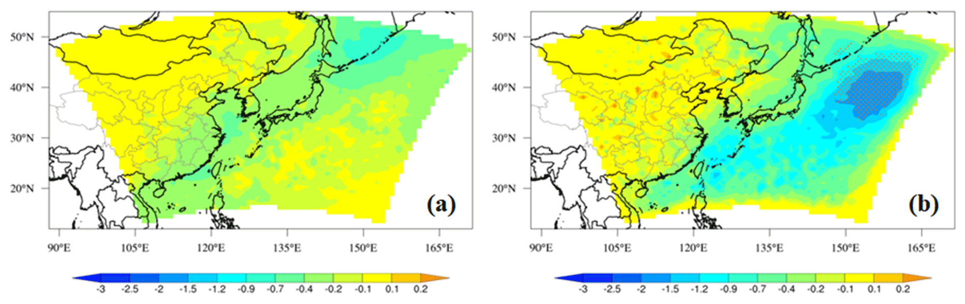
Figure 11 Model-simulated annual mean (a) direct radiative effect of MOA due to aerosol–radiation interaction (DRE_ari), (b) indirect radiative effect of MOA due to aerosol–cloud interaction (IRE_aci) at the top of atmosphere (TOA) (W m⁻²). Red dot indicates areas where the difference is statistically significant at the 99 % confidence level according to a two-tailed t test.

Figure 11b shows the annual mean MOA IRE_aci in the study domain, which was similar in magnitude and distribution pattern to IRE_MOA (Fig. 10f), but it distributed unevenly in the domain with some positive values exceeding 0.2 W m⁻² over both the western Pacific and the continent. IRE_aci of MOA was statistically significant at the 99 % confidence level over the NWP region. The atmospheric response and adjustment induced by IRE_MOA could be somewhat stronger than that by DRE_MOA with respect to the positive values of IRE_aci up to 0.3 W m⁻² over the continent. The small positive values could be associated with the radiative feedback and atmospheric and cloud adjustment.

The annual and domain average of DRE_ari and IRE_aci over the western Pacific are estimated to be −0.25 and −0.61 W m⁻², respectively; both are somewhat weaker than the DRE_MOA (−0.27 W m⁻²) and IRE_MOA values (−0.66 W m⁻²).

5 Conclusions

The organic aerosols of marine origin over the western Pacific Ocean of East Asia was investigated by an online coupled regional climate chemistry model RIEMS-Chem for the year 2014. Emissions and relevant processes of marine MPOA, isoprene, and monoterpene were incorporated into RIEMS-Chem. A wide variety of observational datasets from EANET, CNEMC, and AERONET networks, cruise measurements, and previous publications were collected for model validation. The modelled SOA from marine VOC sources was also compared with secondary organic tracers measured by research cruise. The model performed well for PM_2.5 and PM₁₀ in a marine environment, producing overall correlation coefficients and NMBs of 0.61$/$0.70 and 12 % $/-$7 % for PM_2.5 concentration and 0.65 $/$ 0.65 and −5 % $/-$1 % for PM₁₀ concentration at the EANET/CNEMC sites, respectively. The model reasonably reproduced the spatial distribution and temporal variation in BC and OC concentrations along cruise tracks and at islands over the western Pacific, with the correlation coefficients and NMBs being 0.6–0.75 and −28 %–3 % for OC, respectively. The modelled OC concentration was apparently improved while taking marine organic aerosols into account. The model results clearly showed an increasing contribution of marine organic aerosols to total OC mass concentration from the marginal seas of China to remote oceans. Organic aerosol mass of marine origin was dominated by MPOA because MSOA produced by marine isoprene and monoterpene emissions was about 1–2 orders of magnitude lower than MPOA. The model simulates AOD reasonably well at the seven coastal or island AERONET sites, with an overall correlation coefficient of 0.54 and an NMB of −6 %.

High MPOA emission mainly occurred over the marginal seas of China (EYB) and the northern parts of western Pacific northeast of Japan (NWP). For the western Pacific, MPOA emission reached the maximum in SON, followed by those in DJF and MAM, and the minimum in JJA, with an annual and domain average emission rate of $\mathrm{0.16}\times {\mathrm{10}}^{-\mathrm{2}}$ $\mathrm{\mu }\mathrm{g}{\mathrm{m}}^{-\mathrm{2}}{\mathrm{s}}^{-\mathrm{1}}$. The combination of chl a concentration and sea salt emission flux determined the seasonality of MPOA emission. The annual MPOA emission for the year 2014 was estimated to be 0.78 Tg yr⁻¹ over the western Pacific.

Consistent with the distribution pattern MPOA emission, high MOA concentration mainly distributed over the EYB and NWP, with an annual and domain mean concentration of 0.27, 0.48, and 0.59 µg m⁻³ over the western Pacific, the EYB, and the NWP regions, respectively. MOA concentration was highest in MAM and lowest in DJF, with the seasonal and domain mean values of 0.37 and 0.21 µg m⁻³, respectively, over the western Pacific. The seasonality of MOA concentration was determined by the combined effect of MPOA emission and dry and wet depositions.

On average, the annual mean percentage contribution of MOA to total OA mass was 26 % over the western Pacific, with the largest seasonal mean contribution of 32 % in SON and the lower ones in DJF (24 %) and JJA (23 %). Over the NWP, the domain average contribution of MOA to OA could be as high as 42 % in terms of annual mean and approaching 52 % in MAM; however, over the EYB, the annual mean contribution was just 13 % and the percentage contribution was even reduced to 6 % in JJA. This indicated that the relative importance of MOA in total OA concentration increased with the distance away from the East Asian continent. MSOA concentration was approximately 1–2 orders of magnitude lower than MPOA, with the simulated annual and regional mean MSOA being 2.2 ng m⁻³ and the maximum daily mean value up to 28 ng m⁻³ in summer over the western Pacific.

An annual/oceanic mean all-sky DRE_MOA of −0.27 W m⁻² at the TOA was estimated over the western Pacific, which was about 40 % of the IRE_MOA (−0.66 W m⁻²). The domain mean IRE_MOA was strongest in spring (−0.94 W m⁻²) and weakest in summer (−0.36 W m⁻²) over the western Pacific, and the monthly mean IRE_MOA can reach −5 W m⁻² in the NWP region east of Japan in April. The changes in MOA concentration and cloud amount both contributed to the seasonality of IRE_MOA. In terms of annual and oceanic mean over the western Pacific, MSOA just contributed approximately 1 % of the IRE_MOA. IRE_MOA was generally larger than the IRE due to sea salt on average. The annual and oceanic mean IRE due to sea spray aerosols (MOA + sea salt) was approximately 12 % of that due to total aerosols over the western Pacific, but this ratio can increase up to 19 % in autumn in the NWP region. The estimation of IRE_MOA was sensitive to MOA properties, which apparently decreased, while a smaller geometric mean radius together with a lower solubility and a larger molecule weight were assigned for MOA. Overall, the indirect radiative effect of MOA was larger than the direct radiative effect and had a nonnegligible impact on radiation budget and cloud over the western Pacific. The direct and indirect radiative effect considering atmospheric feedback and adjustment were estimated as well, which was similar in magnitude to the DRE_MOA and IRE_MOA, with a few positive changes in shortwave radiation fluxes in some locations.

While this study presents new insights into the seasonal variation and annual means of emissions, concentrations, and radiative effects of MOA in the western Pacific, it is still subject to some uncertainties as follows: (1) the properties of marine organic aerosols, including size distribution, molecular weight, solubility, and surfactant amount are still poorly characterized, which are crucial to aerosol activation, dry deposition, and wet scavenging; (2) the sources and chemical formation processes of marine organic aerosols including secondary organics are highly complex and poorly understood and represented in the model; (3) the indirect effects of MOA in this study is for warm stratiform cloud. Further research on MOA sources, properties, chemical processes, and climatic impacts will be conducted together with the advances in both field experiments (integrated cruise, aircraft, and satellite observations) and model development in the future.