Six years of continuous carbon isotope composition measurements of methane in Heidelberg (Germany) – a study of source contributions and comparison to emission inventories

Mitigation of greenhouse gases requires a precise knowledge of their sources at both global and regional scales. With improving measurement techniques, in situ δ(¹³C,CH₄) records are analysed in a growing number of studies to characterise methane emissions and to evaluate inventories at regional and local scales. However, most of these studies cover short time periods of a few months, and the results show a large regional variability. In this study, a 6-year time record of in situ δ(¹³C,CH₄), measured with a cavity ring-down spectroscopy (CRDS) analyser in Heidelberg, Germany, is analysed to obtain information about seasonal variations and trends of CH₄ emissions. The Keeling plot method is applied to atmospheric measurements on different timescales, and the resulting source contributions are used to evaluate the CH₄ emissions reported by two emission inventories: the Emissions Database for Global Atmospheric Research (EDGAR v6.0) and the inventory of the State Institute for the Environment Baden-Württemberg (LUBW). The mean isotopic carbon source signature for the Heidelberg catchment area derived from atmospheric measurements is $(-\mathrm{52.3}\pm \mathrm{0.4})$ ‰ and shows an annual cycle with 5.8 ‰ more depleted values in summer than in winter. This annual cycle can only be partly explained by seasonal variations in the ¹³C-enriched emissions from heating and reveals strong seasonal variations in biogenic CH₄ emissions in the Heidelberg catchment area, which are not included in EDGAR v6.0. The comparison with emission inventories also shows that EDGAR v6.0 overestimates the CH₄ emissions from less depleted sources. In situ CH₄ isotope analysers at continental and urban monitoring stations can make an important contribution to the verification and improvement of emission inventories.

1 Introduction

One of the most challenging problems of our time is global warming. To limit the negative impacts associated with climate change, the 2015 UN Paris Agreement on Climate Change has set the goal to limit the mean global temperature increase to below 2 °C, preferably to 1.5 °C, compared to pre-industrial level (UNFCCC, 2015). In 2021 the United States, the European Union, and other countries launched the Global Methane Pledge with the goal to reduce global methane emissions. This initiative recognised the short lifetime of methane (CH₄) of only 9.1 to 11.8 years (IPCC, 2023), allowing for a more rapid effect on atmospheric CH₄ mole fraction after reducing CH₄ emissions.

On a global scale several studies have analysed atmospheric carbon isotope ratios in methane, in addition to CH₄ mole fractions to constrain emission budgets and to explain observed atmospheric trends in mole fraction (e.g. Nisbet et.al, 2016, 2019; Schaefer, 2016, 2019; and Lan et al., 2021). This is possible, since each source type has a different isotopic signature depending on the production processes and origin.

The isotopic composition of methane δ(¹³C,CH₄), hereafter abbreviated as δ(¹³CH₄), is described with the δ-notation, using the isotope ratio R, and is typically given in ‰.

$$\begin{array}{}\text{(1)}& \mathit{\delta }={\displaystyle \frac{R_{\mathrm{sample}}}{R_{\mathrm{standard}}}}-\mathrm{1}\end{array}$$

The isotope ratio R is the ratio between the abundance of the rare isotope and the abundance of the abundant isotope, here between the heavy and light stable isotopes. The international reference standard for reporting δ(¹³CH₄) is the Vienna Pee Dee Belemnite (VPDB; 0.0111802 ± 0.0000028, Werner and Brand, 2001).

CH₄ is emitted from anthropogenic and natural sources, which are grouped in three different categories according to the production processes. Biogenic CH₄ is produced under anaerobic conditions due to degradation of organic matter (typically −70 ‰ to −55 ‰; IPCC, 2013). Biogenic CH₄ sources are wetlands, ruminants, landfills, and wastewater treatment plants. Thermogenic CH₄, like that in natural gas, is formed on geological timescales out of organic matter and is less depleted than biogenic CH₄ (typically −45 ‰ to −25 ‰; IPCC, 2013). Pyrogenic CH₄ is formed during the incomplete combustion of organic matter, such as biomass burning, and is typically more enriched (typically −25 ‰ to −13 ‰; IPCC, 2013) compared to biogenic and thermogenic CH₄. Studies by Sherwood et al. (2017, 2021) and Menoud et al. (2022) show that δ(¹³CH₄) of the different source categories are not always as distinct as indicated above. They give much larger ranges for the different source categories, which also overlap as a result. Especially for fossil but also for biogenic sources large regional differences occur.

The knowledge of the spatial and temporal variation of CH₄ emissions around the world, and their composition from different types of sources, is important to reduce CH₄ emissions effectively and to understand the influence of different CH₄ sources on climate change. Also on a local and regional scale, the measurement of atmospheric δ(¹³CH₄) provides information about the contribution of different emission sectors to the total CH₄ emissions. Traditionally, δ(¹³CH₄) in the atmosphere is measured by collecting weekly flask or sample bags and analysing them with isotope ratio mass spectrometry (Miller et al., 2002; Fischer et al., 2006; Zazzeri et al., 2015; Röckmann et al., 2016). This method was used by Levin et al. (1999), who analysed and evaluated atmospheric samples integrated over 2 weeks in Heidelberg in the 1990s. With new measurement techniques such as continuous flow isotope ratio mass spectrometry (IRMS), quantum cascade laser absorption spectroscopy (QCLAS), or cavity ring-down spectroscopy (CRDS), the δ(¹³CH₄) values in ambient air can be measured continuously and with high temporal resolutions from a few seconds up to minutes (Eyer et al., 2016; Röckmann et al., 2016; Hoheisel et al., 2019; Rennick et al., 2021).

There is a growing number of studies analysing atmospheric measurements of δ(¹³CH₄) and of CH₄ mole fractions with high temporal resolution. Assan et al. (2018) analysed δ(¹³CH₄) measurements near industrial sites; Röckmann et al. (2016) and Menoud et al. (2020) studied δ(¹³CH₄) in rural areas in the Netherlands. CH₄ measured at urban stations, however, originates from heterogeneously distributed sources including waste management, natural gas distribution systems, heating, transport, and agriculture. The corresponding emissions vary strongly in their isotopic ¹³C–CH₄ composition and make the analysis and interpretation of CH₄ emissions in cities more difficult (Menoud et al., 2021). However, isotope studies with high-resolution measurements can also contribute to revealing possible inconsistencies in emission inventories in urban areas. By analysing a 2-year time series of δ(¹³CH₄) in London, Saboya et al. (2022) demonstrated that emissions from natural gas leaks are underestimated in both the UK National Atmospheric Emissions Inventory (UK NAEI) and the Emissions Database for Global Atmospheric Research (EDGAR).

At the urban station Heidelberg, the atmospheric CH₄ mole fraction and isotopic composition δ(¹³CH₄) have been measured continuously with a CRDS analyser since 2014. This measurement device enables the analysis of CH₄ and δ(¹³CH₄) at high temporal resolution of a few seconds. To our knowledge, our time series is the longest in situ δ(¹³CH₄) record, with high temporal resolution, reported to date. CH₄ emissions around Heidelberg originate from different sources due to the urban region with rural surroundings. The regional emission inventory from the State Institute for the Environment Baden-Württemberg (LUBW – Landesanstalt für Umwelt Baden-Württemberg) classified the CH₄ emissions for 2016 for the Heidelberg region to the following main sectors: agriculture (30 %), waste management (30 %), and natural gas distribution systems (28 %) (LUBW, 2016).

In this study, a continuous 6-year time series between 2014 and 2020 of the atmospheric CH₄ mole fraction and δ(¹³CH₄) at the urban station Heidelberg is analysed to identify and understand seasonal and long-term variabilities of regional and local CH₄ sources. Different approaches, such as the moving Keeling plot approach, are used to determine the contribution of different sectors to CH₄ total emissions in the catchment area of Heidelberg. These results are then compared to a regional emission inventory provided by LUBW and the emission database EDGAR v6.0. Thus, atmospheric measurements are used to verify the estimated contribution of the different emission sectors to CH₄ emissions in the emission inventories.

2 Methods

2.1 Site description

Heidelberg (≈ 159 000 inhabitants) is located in the south-west of Germany and in the north of the state Baden-Württemberg. It is situated in the Upper Rhine Plain on the edge of the low mountain range Odenwald (Fig. 1). Therefore, the north-east is less urban and more forested. More agricultural and urban areas are in the Upper Rhine Plain from the north-west to south-east. The industrial cities of Mannheim (≈ 312 000 inhabitants) and Ludwigshafen (≈ 172 000 inhabitants) are 15 to 20 km north-west of Heidelberg. Due to its location within industrial, urban, agricultural, and rural areas, CH₄ emissions measured in Heidelberg can originate from biogenic (e.g. dairy cows, wastewater treatment plants), thermogenic (e.g. natural gas), and even pyrogenic (e.g. traffic) sources. The CH₄ mole fraction and δ(¹³CH₄) measurements are done at the Institute of Environmental Physics (IUP – Institut für Umweltphysik, 49°25^′2^′′ N, 8°40^′28^′′ E, 116 m a.s.l.).

Figure 1 Location of the measurement station in Heidelberg at the Institute of Environmental Physics (IUP – Institut für Umweltphysik) (map data from © Google Earth).

2.2 Experimental setup

Since April 2014, a cavity ring-down spectroscopy (CRDS) G2201-i analyser (Picarro, Inc., Santa Clara, CA) has been continuously measuring the dry-air mole fraction of CH₄ and its ${}^{\mathrm{13}}\mathrm{C}{/}^{\mathrm{12}}$C ratio in ambient air with a temporal resolution of a few seconds. The intake for these ambient air measurements is located on the roof of the Institute for Environmental Physics (IUP) in Heidelberg, 30 m above ground. Several studies have shown that the internal water correction, especially for δ(¹³CH₄), is insufficient for this type of analyser (Rella et al., 2015; Hoheisel et al., 2019), and air drying is required for precise measurements. Thus, a cold trap cooled by a cryostat dries the air before it enters the CRDS analyser through a 16-way rotary valve (model: EMT2CSD16UWE, VICI Valco, Switzerland). The gas flow through the analyser is typically about 80 mL min⁻¹ and is monitored by an electronic flow meter (model: 5067-0223, Agilent Technologies, Inc., Santa Clara, CA). Every 5 h, the ambient air measurement is interrupted to analyse calibration and quality control gases for 20 min each. The schematic of the laboratory setup is shown in Fig. 2.

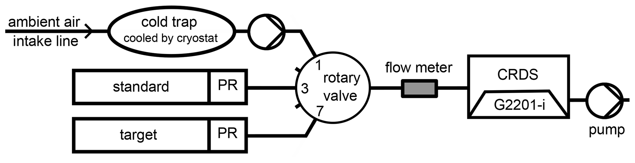
Figure 2 Experimental setup to measure CH₄ mole fraction and δ(¹³CH₄) in ambient air in Heidelberg.

2.3 Data treatment

The G2201-i analyser records CH₄ and the isotopic composition δ(¹³CH₄) every 3.7 s. These high temporal resolution data are averaged to 1 min values. Before analysing these minutely CH₄ and δ(¹³CH₄) values of ambient air, artefacts, outliers, and invalid data are identified and flagged. These include periods of technical problems, work on the experimental setup such as replacing the cold trap, and the first 5 min after a change of sample gas to account for flushing of the cavity.

The 1 min CH₄ mole fractions and the isotopic composition of CH₄ are calibrated with a single-point calibration using the calibration measurements carried out every 5 h. In August 2019, the calibration cylinder had to be replaced (see Table A1). The CH₄ mole fraction measurements are reported on the WMO X2004A scale (Dlugokencky et al., 2005) in nmol mol${}^{-\mathrm{1}}={\mathrm{10}}^{-\mathrm{9}}$ (nanomole per mole of dry air). The measurements of the isotopic compositions of CH₄ are traced to the Vienna Pee Dee Belemnite (VPDB) isotopic scale (Sperlich et al., 2016). Hence, in 2014 and 2019, the calibration cylinders were analysed with the gas chromatography (GC) system in Heidelberg (Levin et al., 1999), and the δ(¹³CH₄) values were measured by the Stable Isotope Laboratory at Max Planck Institute for Biogeochemistry (MPI-BGC) in Jena.

2.4 Instrumental performance

The instrumental precision of the analyser was determined in 2013 and 2019 by performing measurements on different gas cylinders for at least 12 h each. The Allan standard deviation determined from these measurements can be used as a measure of the repeatability of a measurement over a certain period of time. The Allan standard deviation of atmospheric CH₄ is below 0.11 nmol mol⁻¹ even for the high-resolution 1 min data. For an averaging interval of 15 min, corresponding to the calibration and target gas measurements, and CH₄ mole fractions between 1922 nmol mol⁻¹ and 2004 nmol mol⁻¹, the Allan standard deviation of CH₄ and δ(¹³CH₄) is 0.08 nmol mol⁻¹ and 0.24 ‰, respectively (see Fig. A1). The long-term reproducibility of the CRDS G2201-i analyser, i.e. the standard deviation of the target gas measurements performed between 2014 and 2020, is 0.2 nmol mol⁻¹ for CH₄ and 0.3 ‰ for δ(¹³CH₄) (see Fig. A2).

Six intercomparison cylinders with air samples from Neumayer Station in Antarctica were measured with our CRDS G2201-i analyser to validate the measurement accuracy. These cylinders had already been analysed by the MPI-BGC within the framework of an interlaboratory comparison (Umezawa et al., 2018). The average difference in δ(¹³CH₄) between our results and the MPI-BGC measurements is (0.02 ± 0.05) ‰ (see Table A2).

3 Results and discussion

3.1 Continuous CH₄ mole fraction and δ(¹³CH₄) measurements

Atmospheric CH₄ mole fraction and δ(¹³CH₄) were measured continuously with a CRDS analyser in Heidelberg between April 2014 and May 2020. Figure 3 shows the daily mean CH₄ mole fractions, which vary between 1890 and 2310 nmol mol⁻¹, with higher values in winter than in summer. The corresponding isotopic composition δ(¹³CH₄) ranges from −49.3 ‰ to −47.3 ‰.

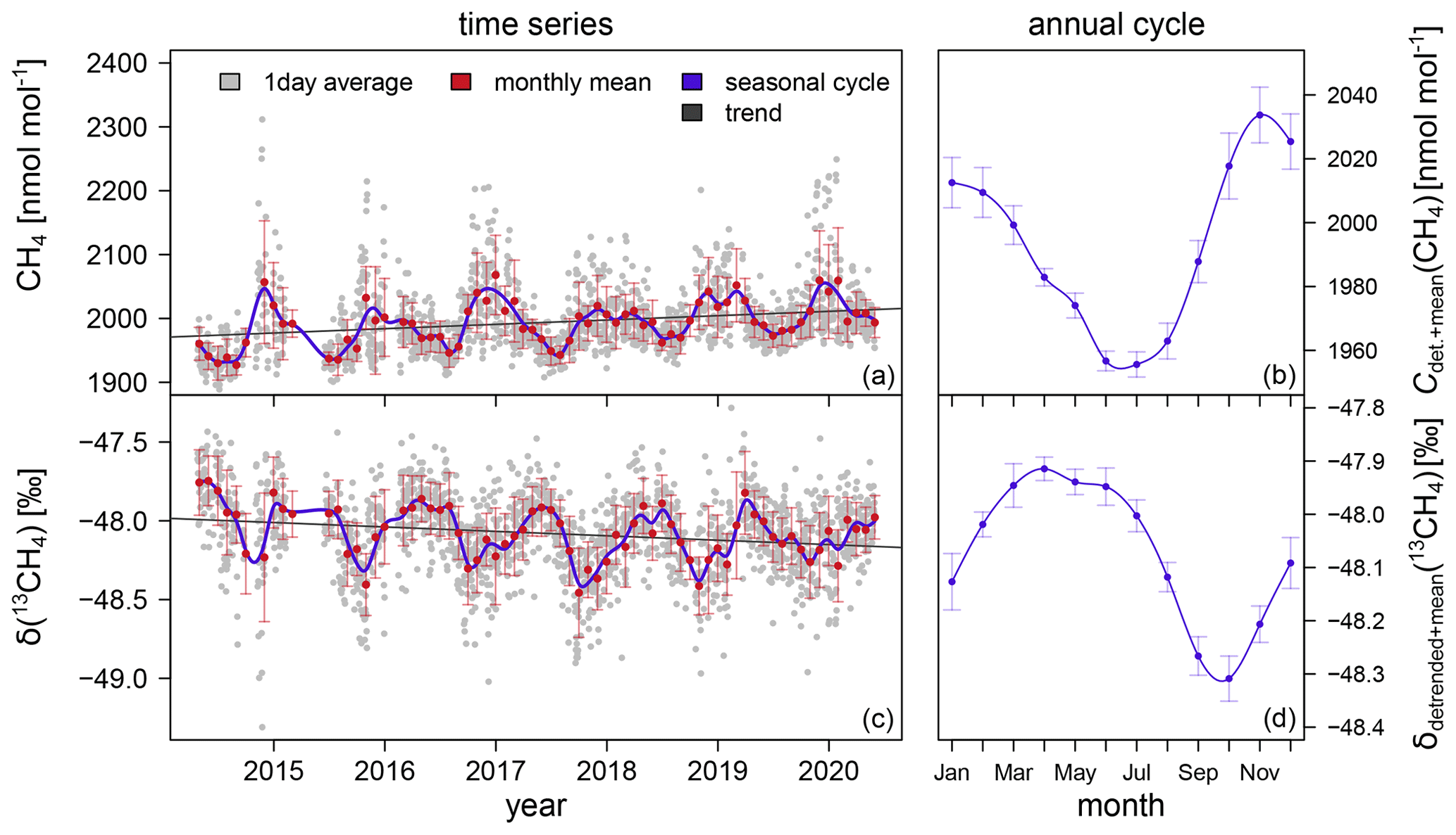
Figure 3 Atmospheric CH₄ mole fraction and δ(¹³CH₄) measured in Heidelberg and corresponding annual cycles. The monthly mean values and standard deviation (red) are calculated from the daily averages (grey). The mean annual cycle with the standard errors are shown in blue. Note that the y axis ranges are not the same for (a, c) and (b, d).

The digital filter curve fitting program CCGCRV¹ developed by Kirk Thoning (Earth System Group, Earth System Laboratory (CCG/ESRL), NOAA, Thoning et al., 1989) is applied to the monthly average data to analyse the trend and annual cycle of CH₄ and δ(¹³CH₄). CCGCRV can be used to decompose a time series into a trend and a detrended seasonal cycle by fitting a polynomial equation combined with a harmonic function to the data and applying a filter to the residuals. In this study, we used three polynomial terms and four annual harmonic terms. The short- and long-term cutoff values for the low-pass filter are 80 and 667, respectively. Between 2014 and 2020, the CH₄ mole fraction increases by (6.8 ± 0.3) nmol mol⁻¹ a⁻¹, and δ(¹³CH₄) shows a decreasing trend of (−0.028 ± 0.002) ‰ a⁻¹. Furthermore, CH₄ and δ(¹³CH₄) show strong mean annual cycles (Fig. 3b, d). The maximum of the mean CH₄ mole fraction occurs in late autumn (November). In winter and spring, the mole fraction decreases slightly until it reaches a minimum in late summer (June to July). The amplitude (peak-to-peak height) is 78 nmol mol⁻¹ in CH₄. The annual cycle in atmospheric δ(¹³CH₄) has a mean amplitude of 0.4 ‰. In early autumn (September to October) the δ(¹³CH₄) values are more depleted than the values in spring (April to May).

In addition to the trend and the annual cycle, the CH₄ mole fraction and δ(¹³CH₄) show diurnal variations. The mean diurnal cycles for different seasons are presented in Fig. 4. In the afternoon (15:00–16:00 UTC), the overnight increase in the CH₄ mole fraction begins due to the lower mixing height. After sunrise, the mole fraction decreases strongly due to radiation-induced mixing and thus an increase of the mixing height. The mean diurnal cycles show strong seasonal differences with larger variations in summer (52 nmol mol⁻¹) and weaker ones in winter (21 nmol mol⁻¹). Since the diurnal cycle is strongly driven by the sun, the earlier sunrise and later sunset in summer compared to winter is additionally noticeable by the earlier decrease of CH₄ in the morning and the later increase in the afternoon. The diurnal variations of δ(¹³CH₄) show slightly larger amplitudes in summer (0.18 ‰) and autumn (0.16 ‰) than in winter (0.09 ‰) and spring (0.12 ‰). The lowest δ(¹³CH₄) values occur around 07:00 to 10:00 UTC. δ(¹³CH₄) increases during the day to maximum values between 18:00 and 21:00 UTC, before decreasing at night. It seems that, in summer, the depletion in δ(¹³CH₄) in the morning is slightly stronger than in the other seasons.

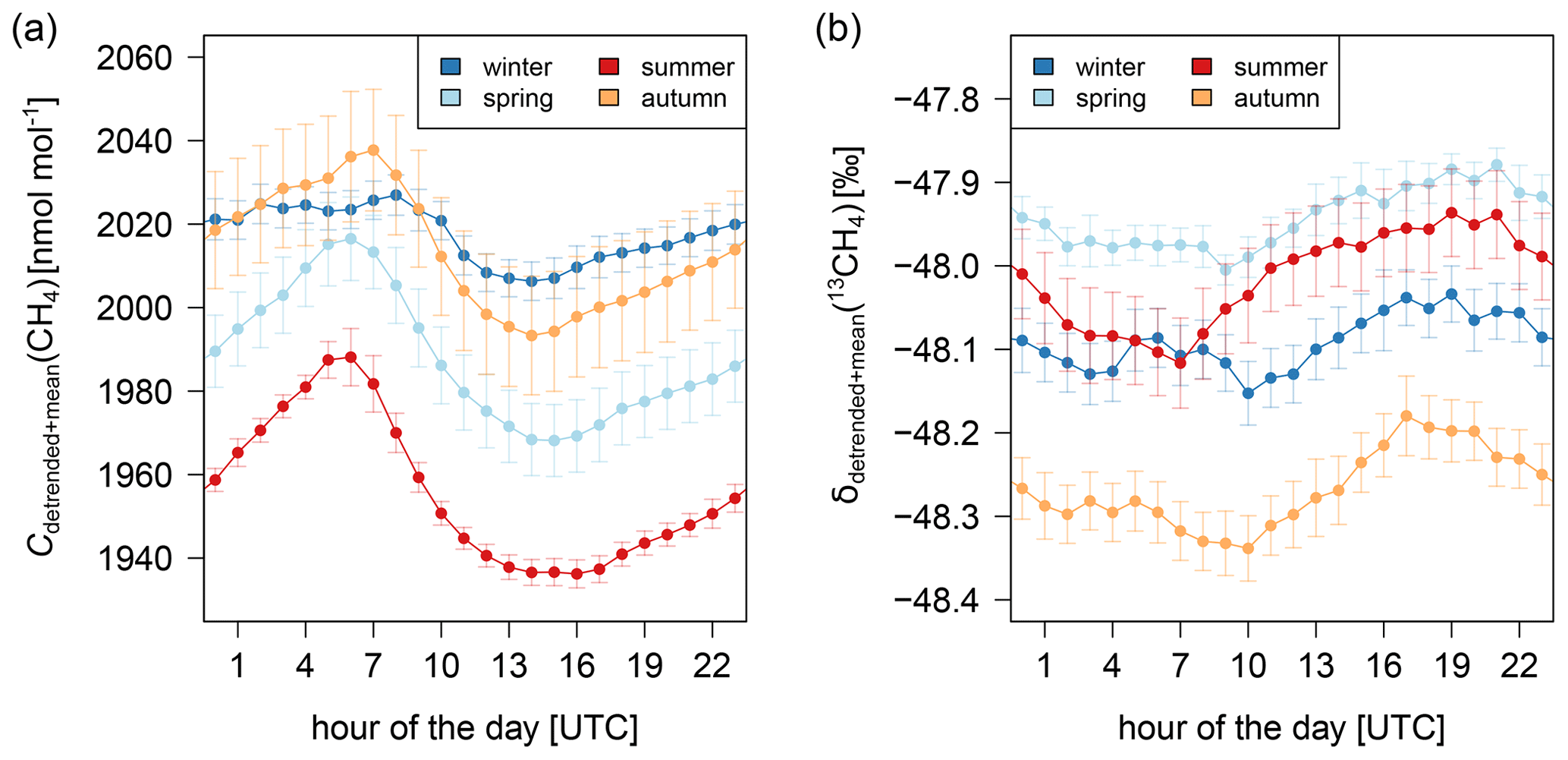
Figure 4 Diurnal cycles of CH₄ (a) and δ(¹³CH₄) (b) in Heidelberg. For each season the diurnal cycles of each month, which are detrended by subtracting the diurnal mean, are averaged, and the mean CH₄ mole fraction or δ(¹³CH₄) value for each season is added.

3.2 Comparison of δ(¹³CH₄) with background and previous measurements

In Heidelberg, the CH₄ mole fraction and δ(¹³CH₄) were measured with a GC-IRMS system and from flask samples integrated over 2 weeks between 1992 and 1997 (Levin et al., 1999). Since the previous CH₄ mole fractions were reported on the CMDL83 scale, we take into account that the CH₄ mole fractions measured on the new WMO 2004 scale are a factor of (1.0124 ± 0.0007) larger (Dlugokencky et al., 2005). Figure 5 shows CH₄ and δ(¹³CH₄) from the two time periods (1992–1998, 2014–2020) for which δ(¹³CH₄) measurements were done in Heidelberg. In addition to the Heidelberg measurements, monthly data from the marine background station Mace Head Observatory (Lan et al., 2022; Michel et al., 2022) are shown. The Mace Head Observatory (53°19^′36^′′ N, 8.4 m a.s.l.) is located on the west coast of Ireland and measures the maritime background mole fraction when air is coming from the ocean. The isotopic composition measured at Mace Head by the Institute of Arctic and Alpine Research (INSTAAR) of the University of Colorado has to be subtracted by an offset of 0.28 ‰ to take into account the inter-comparison offset among the laboratories INSTAAR and MPI-BGC (Umezawa et al., 2018).

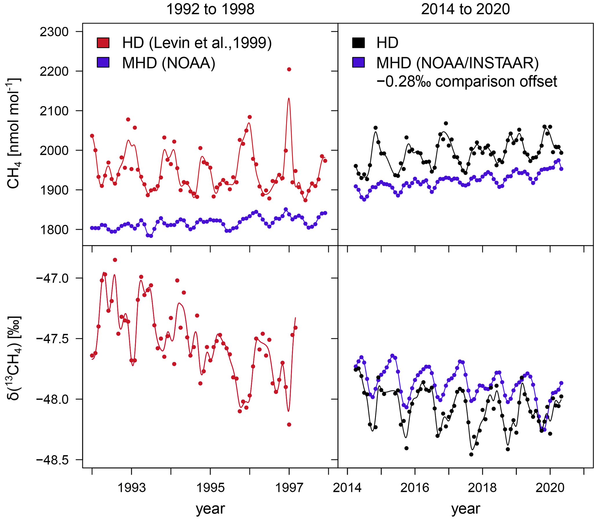
Figure 5 CH₄ mole fraction and δ(¹³CH₄) in Heidelberg from 1992 to 1998 (Levin et al., 1999) and between 2014 and 2021. In addition, measurements done at the marine background station Mace Head (Lan et al., 2022; Michel et al., 2022) are shown in blue.

Again the curve fitting program CCGCRV is applied to the monthly mean values to determine trends and seasonal variabilities. The observed increasing trend in Heidelberg between April 2014 and June 2020 is only slightly smaller than the one in Mace Head. This was different in the 1990s, where the CH₄ mole fraction did not follow the increasing trend observed at the background station Izaña (Levin et al., 1999) or Mace Head. Furthermore, the continental CH₄ excess at Heidelberg (Heidelberg data minus Mace Head data) strongly decreased between the 1990s and recent years (2014–2020) to (70 ± 3) nmol mol⁻¹, which is only half of the value from the 1990s. These observations can be explained by a change in the emission rate in the catchment area of Heidelberg. In the studies by Levin et al. (2011, 2021) the CH₄ fluxes in the catchment area of Heidelberg are calculated with the radon-tracer method. They found a 30 % reduction of CH₄ emissions between 1996 and 2004 and no further systematic trend thereafter. In the 1990s, the δ(¹³CH₄) values in Heidelberg decreased strongly with −0.14 ‰ a⁻¹, while samples from Izaña only showed trends which are more than a factor of 3 smaller (Levin et al., 1999). This difference in the δ(¹³CH₄) trends points to a change in the composition of CH₄ emissions in the catchment area of Heidelberg. Levin et al. (1999) attribute this change to a reduction of CH₄ emissions from fossil sources (mainly coal mining) and from cattle breeding. The situation is different for recent measurements (2014 to 2020). The current Heidelberg data only show a small trend in δ(¹³CH₄) which is similar to the one observed at Mace Head. Therefore, the CH₄ source mixture in the catchment area of Heidelberg seems to have been relatively constant during the last years.

3.3 Isotopic carbon signature of CH₄ sources calculated with atmospheric measurements

CH₄ sources contributing to the atmospheric CH₄ mole fraction have different isotopic carbon source signatures depending on their origin and production process. These isotopic source signatures can range from −13 ‰ to −70 ‰ (Sherwood et al., 2021; Menoud et al., 2022). Therefore, the measured atmospheric δ(¹³CH₄) value strongly depends on the CH₄ source mixture from regional and local sources. That makes it possible to analyse the CH₄ sources in the Heidelberg catchment based on the measured atmospheric CH₄ mole fraction in combination with the observed atmospheric isotopic composition δ(¹³CH₄). In most cases, an increase in atmospheric CH₄ mole fraction will be caused by a mixture of CH₄ emitted from different sources. Thus, from the atmospheric measurements, one usually does not obtain information about a single source but the average isotopic signature of several contributing sources depending on their respective emission rate.

3.3.1 Determination of mean isotopic carbon source signatures

In this study we use the Keeling plot method (Keeling, 1958, 1961) in combination with the York fit (York et al., 2004) to determine the mean isotopic carbon source signature in the catchment area of Heidelberg. This method is applied to the 1 min averages of CH₄ and δ(¹³CH₄) for which the Allan standard deviation is used as a measure of instrumental uncertainty. The Keeling plot method uses the linear relationship between δ_obs and $\mathrm{1}/C_{\mathrm{obs}}$, where C and δ refer to CH₄ and δ(¹³CH₄):

$$\begin{array}{}\text{(2)}& {\mathit{\delta }}_{\mathrm{obs}}={\displaystyle \frac{\mathrm{1}}{C_{\mathrm{obs}}}}\cdot C_{\mathrm{bg}}\cdot \left({\mathit{\delta }}_{\mathrm{bg}}-{\mathit{\delta }}_{\mathrm{s}}\right)+{\mathit{\delta }}_{\mathrm{s}}.\end{array}$$

Here, the indices obs, bg, and s denote observed, background, and source values. The York fit was chosen as this method minimises the weighted distance between the data points and the fitted line, taking into account uncertainties in both x and y coordinates.

The uncertainty of the source signature determined with the Keeling plot method and the York fit strongly depends on the precision of the analyser and the peak height of CH₄ (Hoheisel et al., 2019). To achieve accurate results for the mean isotopic carbon source signatures, we apply two criteria to our data: the CH₄ range of the data set, to which the Keeling plot is applied, has to be larger than 100 nmol mol⁻¹, and the fit error on the slope of the regression line has to be smaller than 2.5 ‰.

Another method to determine the mean isotopic carbon source signature is derived by Miller and Tans (2003). For comparison, we also determined the mean isotopic source signatures of CH₄ with the Miller–Tans method (Miller and Tans, 2003, Eq. 5), which uses the linear relationship between δ_obs⋅C_obs and C_obs and where the background values can remain unknown:

$$\begin{array}{}\text{(3)}& {\mathit{\delta }}_{\mathrm{obs}}\cdot C_{\mathrm{obs}}=C_{\mathrm{bg}}\cdot \left({\mathit{\delta }}_{\mathrm{bg}}-{\mathit{\delta }}_{\mathrm{s}}\right)+{\mathit{\delta }}_{\mathrm{s}}\cdot C_{\mathrm{obs}}.\end{array}$$

In our case, there is no difference between the Keeling plot and the Miller–Tans method, when using the York fit. The compatibility of these methods was also shown by Zobitz et al. (2006) for CO₂ and Hoheisel et al. (2019) for CH₄.

Different approaches are tested for the choice of timescale (month, night, moving interval) for which the mean isotopic carbon source signature for Heidelberg should be calculated. Depending on the timescale, the Keeling plot method is applied to different data subsets (each month, each night, moving interval). Larger time intervals of 1 month have the advantage that the CH₄ mole fractions cover a large range, which increases the precision of the results of the regression line. On the other hand, uncertainties occur since the background is probably not constant over the entire time period, which can be assumed for shorter time intervals of a few hours. The three most promising approaches used in this study are the monthly, the night-time, and the moving Keeling plot approach. In the monthly approach, the Keeling plot method is applied to the 1 min average data of each month of each year. In the night-time approach, the Keeling plot method is applied to the 1 min average data between 17:00 and 07:00 CET. This approach uses the night-time increase in the CH₄ mole fraction caused by the accumulation of CH₄ emissions in the lower boundary layer. Therefore, we determine the mean isotopic carbon source signature of the contributing CH₄ sources for each night. In order to achieve meaningful results, only nocturnal data sets that fulfil our two criteria (CH₄ range >  100 nmol mol⁻¹, regression fit error for the slope <  2.5 ‰) are used. This is the case for 21 % of the night data sets. We can therefore determine the mean isotopic carbon source signature in the catchment area of Heidelberg for 460 nights.

Due to the high temporal resolution of our CH₄ mole fraction and δ(¹³CH₄) measurements, we can go one step further and determine the isotopic carbon source signatures with a moving Keeling plot approach similar to the moving Keeling plot or moving Miller–Tans methods used by Röckmann et al. (2016), Menoud et al. (2020), Assan et al. (2018), or Saboya et al. (2022). Since we are interested in short-term events, a time window with a fixed length of 1 h is shifted over the 1 min average data set with time steps of 1 min. Thus, for each minute t_i, the mean isotopic carbon source signature is calculated from a 1 h time period centred on t_i using the Keeling plot method and the York fit. Again only those results which fulfil our two criteria of a CH₄ range larger than 100 nmol mol⁻¹ during the time window and a fit error of the slope smaller than 2.5 ‰ are used. If these criteria for t_i are not achieved, the result for t_i calculated with a time window 1 h longer is used. This continues until both criteria are fulfilled or the length of the time window reaches 12 h. If the criteria are still not met for the 12 h time interval, the result is excluded. With the moving Keeling plot approach, we achieve results for 18 % of the 1 min average data. To take into account that several of the mean isotopic source signatures determined for each minute may describe the same event, an average is taken over each hour.

3.3.2 Monthly averages and annual cycle of the mean isotopic carbon source signatures

Figure 6a shows the monthly averaged values of the mean isotopic carbon signatures of the CH₄ sources in the Heidelberg catchment area, which were determined using the monthly (black), night-time (blue), and moving Keeling plot (red) approaches. The monthly mean isotopic carbon source signatures vary between −61.5 ‰ and −42.3 ‰ and show similar results for the three different approaches. The average mean isotopic carbon source signature of CH₄ in Heidelberg for the whole time period of 6 years is (−52.3 ± 0.3) ‰ (mean ± standard error of the mean), calculated with the moving Keeling plot approach. The result from the night-time approach is $(-\mathrm{52.3}\pm \mathrm{0.4})$ ‰ and does not differ significantly from the moving Keeling plot approach. The result from the monthly approach is $(-\mathrm{53.9}\pm \mathrm{0.3})$ ‰ and is only slightly more depleted than the results from the other two approaches. Thus, the average mean isotopic source signature of CH₄ is more depleted than the mean δ(¹³CH₄) value in the atmosphere in Heidelberg (−48.07 ± 0.02) ‰.

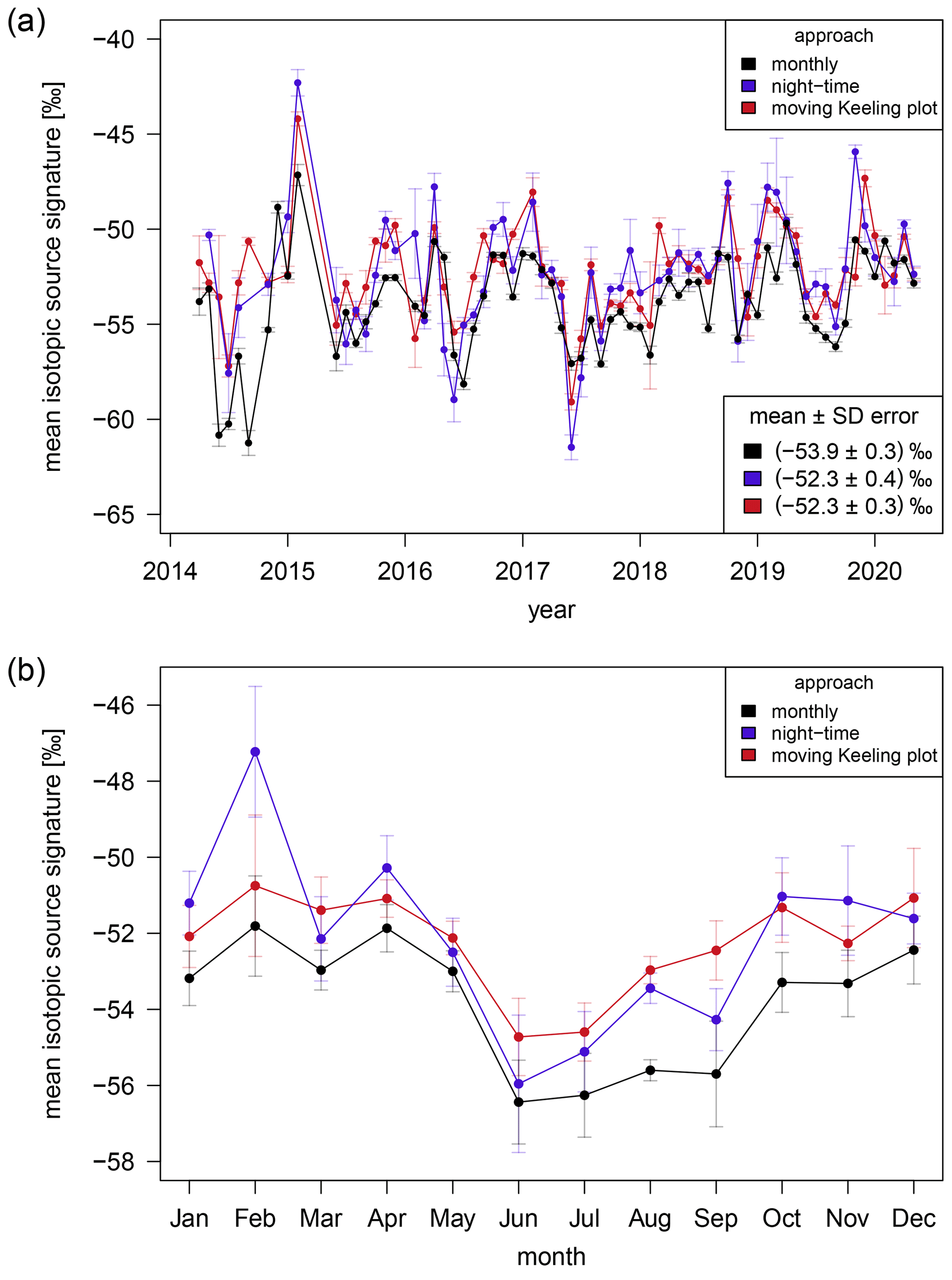
Figure 6 The monthly averages (a) and the annual cycle (b) of the mean isotopic carbon source signatures of CH₄ in the catchment area of Heidelberg between April 2014 and May 2020. The monthly (black), the night-time (blue), and the moving Keeling plot (red) approach are used for the determination. The error bars correspond to the standard deviations.

Since the determined mean isotopic source signature is low and close to what could be expected if biogenic sources (typically between −55 ‰ and −70 ‰) were dominant, a strong influence from biogenic CH₄ sources, such as waste management and agriculture, in the catchment area of Heidelberg can be assumed.

In comparison, the mean isotopic source signatures determined for two 5-month measurement campaigns in more rural areas in the Netherlands, where ruminants are a main CH₄ source, were (−60.8 ± 0.2) ‰ (Röckmann et al., 2016) and (−59.55 ± 0.13) ‰ (Menoud et al., 2020). Looking at other studies in urban areas, Menoud et al. (2021) reported an overall source signature of −48.7 ‰ in Kraków (Poland, 6-month campaign), and Saboya et al. (2022) calculated a median isotopic source signature of −41.6 ‰ for London (UK, 2.7 years), indicating that the primary CH₄ sources in London are natural gas leaks. The mean isotopic carbon signature of CH₄ in Heidelberg thus shows a contribution from less ¹³C-depleted sources such as natural gas, heating, and even traffic from the Heidelberg urban area in addition to biogenic emissions. However, neither of these sources appear to be the only main emitter. This is consistent with the emission inventory of the State Institute for the Environment Baden-Württemberg (LUBW, 2016) for the Heidelberg area, which reports one-third of the emissions each from natural gas leakage, the waste sector, or agriculture (see Fig. 8 in Sect. 3.4.1).

Between 2014 and 2020, no significant trend is detectable in the monthly mean isotopic carbon source signatures obtained from all three approaches. Therefore, we assume that the general composition of CH₄ emissions in the Heidelberg catchment area has not changed or has changed only slightly during this period. This finding is different to a previous study by Levin et al. (1999) from the 1990s. They found a change in the δ(¹³CH₄) source signature from (−47.4 ± 1.2) ‰ in 1992/1993 to (−52.9 ± 0.4) ‰ in 1995/1996 and attribute this change to a reduction of CH₄ emissions from fossil sources (mainly coal mining) and from cattle breeding.

Moreover, a commonality between the mean isotopic carbon source signatures calculated with the different approaches is that a strong annual cycle with more depleted values in the summer than in the winter months can be noticed (Fig. 6b). The annual cycles calculated with all three approaches show the most depleted source signatures in June. From June to October the isotopic carbon source signatures increase and stay relatively constant until April. Between April and June a strong decrease in the mean isotopic carbon source signature is visible. This annual cycle clearly indicates that in summer the CH₄ emissions have a larger biogenic share compared to the rest of the year. When analysing each year individually, the majority have a detectable annual cycle, and it is therefore a very well-defined signal that does not arise from one or two very pronounced annual cycles.

3.3.3 Mean isotopic carbon source signatures of individual nights and days

An advantage of the night-time and moving Keeling plot approach compared to the monthly approach is that the mean isotopic carbon source signature of individual nights or days can be studied. Figure 7a shows the histogram of the mean isotopic carbon source signatures of 460 individual nights calculated with the night-time approach, and Fig. 7b displays a similar histogram using the mean isotopic carbon source signatures averaged for each day determined by the moving Keeling plot approach. Most of the CH₄ emissions during one night or day are a mixture from several sources and cannot be attributed to one particular source. When separating the night-time and day source signatures into winter/spring (November to April) and summer/autumn (May to October), a shift in the mean isotopic carbon source signature of approximately 2 ‰ is noticeable. The mean isotopic carbon source signatures of $(-\mathrm{53.5}\pm \mathrm{0.4})$ ‰ or (−53.2 ± 0.2) ‰ in summer/autumn is less depleted than the ones of (−51.1 ± 0.5) ‰ or (−51.3 ± 0.3) ‰ in winter/spring for the night-time or the moving Keeling plot approach, respectively (Fig. 7). This annual cycle is also described in Sect. 3.3.2. Both approaches additionally have in common that our criteria are fulfilled for fewer nights or days in winter than in summer. Only 41 % to 43 % of the determined isotopic carbon source signatures occur between November and April. Since the diurnal variations are usually lower in winter than in summer, more night-time increases have ranges below the chosen threshold of 100 nmol mol⁻¹ and are therefore excluded.

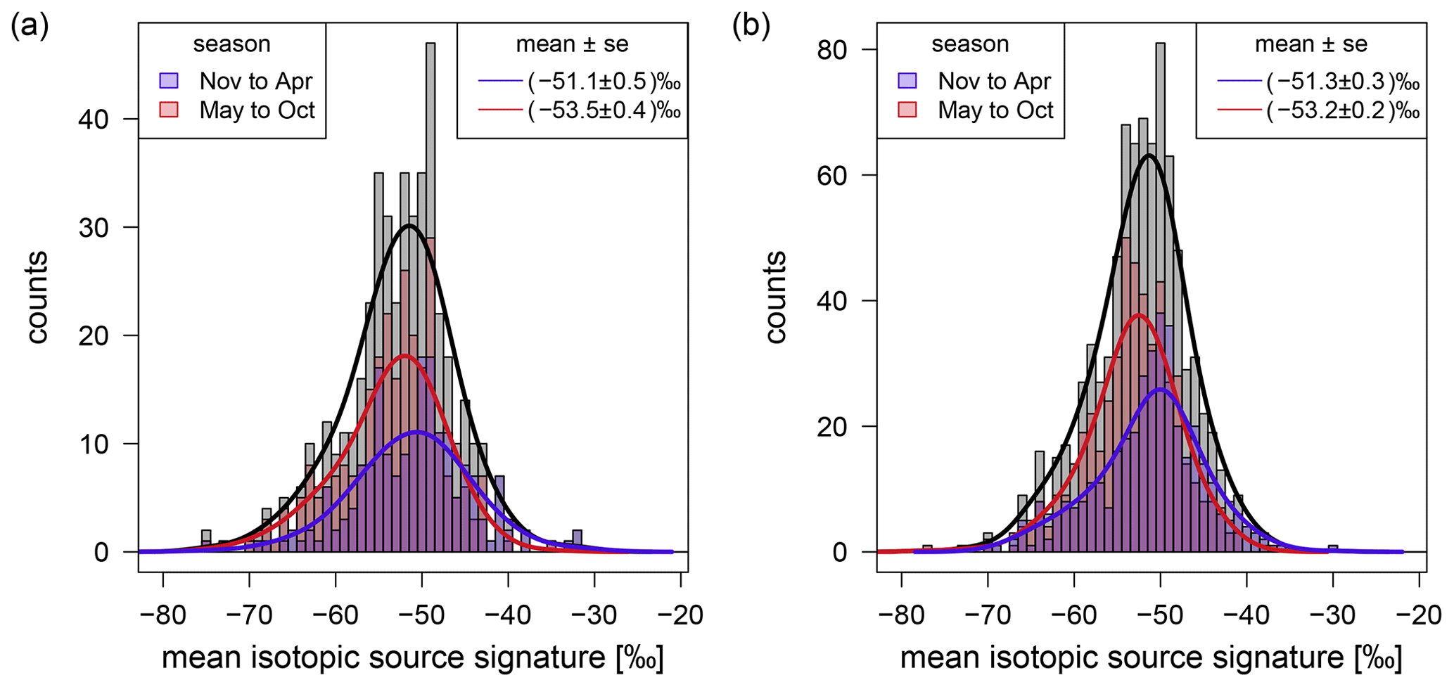
Figure 7 Frequency distribution of the determined mean CH₄ isotopic source signatures of individual nights (a) or daily averages (b) in the catchment area of Heidelberg.

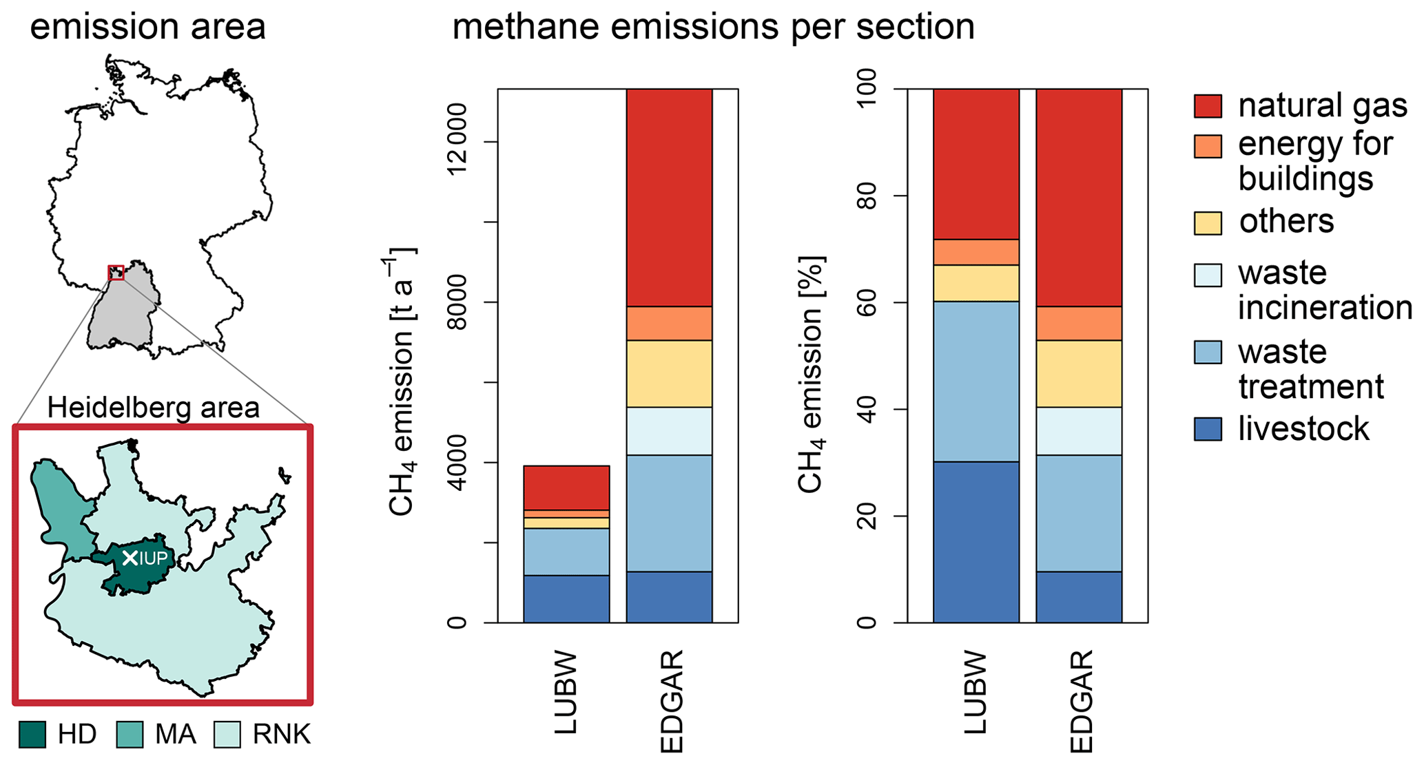
Figure 8 CH₄ emissions and relative proportion of different source categories reported by LUBW (LUBW, 2016 and Manfred Vogel and Thomas Leiber, personal communication, 2019) and calculated from EDGAR v6.0 (Crippa et al., 2021) data for the Heidelberg area, which includes the cities of Heidelberg (HD) and Mannheim (MA) as well as the county Rhein-Neckar-Kreis (RNK).

Furthermore, we determined the diurnal cycle for the mean isotopic carbon source signatures calculated with the moving Keeling plot approach. However, the year-to-year variations are too strong compared to the possible mean diurnal cycle to get reliable results and to exclude the possibility that the noticeable diurnal variations are only an artefact of the averaging. Even though we can analyse the isotopic carbon source signature at timescales below individual months, the precision of our analyser is still too low to interpret diurnal variations. However, the development of new instruments with better precision of isotope measurements will soon make this possible.

3.3.4 Discussion of different approaches

The average mean isotopic carbon source signatures of CH₄ and the annual cycles in Heidelberg calculated with the moving Keeling plot approach or the night-time approach from the whole 6-year time period show no significant differences. This can indicate that the composition of CH₄ sources in Heidelberg is the same during day and night or that the emissions during the night-time increase contribute most in the moving Keeling plot approach.

The monthly approach results in similar monthly mean isotopic carbon source signatures and a similar annual cycle to the other two approaches. The average mean source signature is, however, approximately 1.6 ‰ more depleted than the results from the moving Keeling plot and the night-time approaches (Fig. 6a). The reason for this difference cannot be conclusively resolved in this study. One possibility is that this difference can be caused by the assumption of a constant background over the entire month. Another explanation is that the CH₄ emissions considered in the monthly, night-time, and moving Keeling plot approaches represent different catchment areas and sources, which may cause the difference in the average mean isotopic source signatures. At night, the footprint of Heidelberg is smaller than during the day. In 2018, around 47 % of the surface influence calculated with the Stochastic Time-Inverted Lagrangian Transport (STILT) model (Lin et al., 2003 and Kountouris et al., 2018) for the station Heidelberg is within 50 km at night (18:00 to 03:00 UTC) but within 100 km during the day (06:00 to 15:00 UTC). For these calculations the STILT footprint tools² and the STILT Jupyter Notebook service³ were used. Thus, the monthly approach, which includes daytime data, represents a larger catchment area than the night-time approach. Furthermore, CH₄ emissions from more distant sources show lower and more temporally extended CH₄ peaks in the measured time series than emissions from local and regional sources. In the analysis of small time intervals of several hours, more distant emissions can be excluded by the selection criteria. Thus, the night-time and moving Keeling plot approach probably consider more distant emissions less often than local and regional ones. Excluding nights and time periods that do not fulfil our criteria can of course exclude small pollution events in the night-time and Miller–Tans approach regardless of the distance of the source. These small pollution events, however, contribute to the mean isotopic carbon source signature in the monthly approach, since all 1 min average data points are used there.

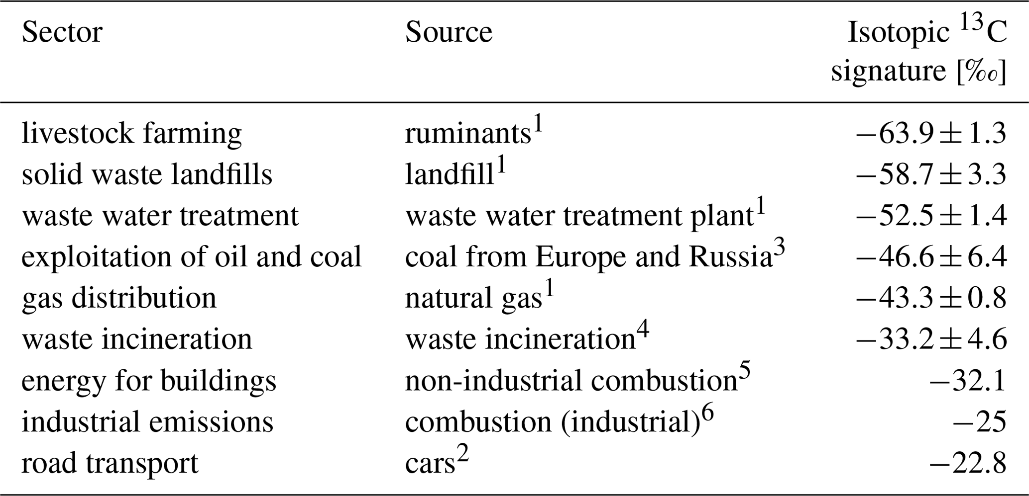
Different CH₄ sources have different isotopic source signatures, which depend on the production process of CH₄. The isotopic source signatures of several sources in the surroundings of Heidelberg are characterised in Hoheisel et al. (2019). Biogenic CH₄ emitted from livestock, landfills, and wastewater treatment is more depleted compared to thermogenic CH₄ from the gas distribution system (see Table 1). Other studies such as Levin et al. (1999), Menoud et al. (2021), and Zazzeri et al. (2017) report isotopic source signatures from combustion processes for traffic, industry, and energy for buildings (see Table 1). This pyrogenic CH₄ is even less depleted than thermogenic CH₄. Since the measurement site in Heidelberg is located in an urban area, the nearby CH₄ sources are more often natural gas leaks, traffic, or emissions from energy for buildings. The more distant sources tend to be in rural areas, so that emissions from landfills and livestock are more prominent. Therefore, the nearby CH₄ emissions are on average less depleted than the more distant biogenic emissions. This agrees well with the more depleted mean isotopic carbon source signature of CH₄ calculated with the monthly approach, in comparison to the night-time approach.

Table 1 Isotopic ¹³C signatures of different CH₄ sources based on measured values in the catchment area of Heidelberg and the literature: (1) Hoheisel et al. (2019), (2) Levin et al. (1993), (3) Sherwood et al. (2017), (4) Widory et al. (2006) (for δ(¹³CO₂)), (5) Menoud et al. (2021), and (6) Zazzeri et al. (2017).

We tested the robustness of the monthly, night-time, and moving Keeling plot approaches by varying the selection criteria. The CH₄ range was set to be 100, 150, or 200 nmol mol⁻¹ and the threshold for the fit error of the slope 2.5 ‰ over 5 ‰ to 10 ‰. All determined monthly mean source signatures show similar results, with an annual cycle containing more biogenic values in summer. The monthly mean isotopic source signatures calculated with different selection criteria show differences between 0.1 ‰ and 0.8 ‰, with standard deviations between 1 ‰ and 3 ‰. Therefore, we choose the CH₄ range of 100 nmol mol⁻¹ as a threshold to include more data sets and 2.5 ‰ as a threshold for the fit error of the slope, and thus the uncertainty of the source signature, to still assure precise results.

Furthermore, several automatic approaches to identify the nocturnal increases for each night in the time series were tested. The determined monthly averaged isotopic carbon source signatures did not vary strongly between the automatic approaches and the one using the fixed time window. Since the automatic approaches did not correctly identify the CH₄ increase for all nights, we chose the same fixed time interval between 17:00 and 07:00 CET for the nightly increase of CH₄ for each day. Also, varying the fixed time interval does not lead to any relevant changes in the monthly averaged mean isotopic carbon source signatures. In addition, we tested a more common method for the moving Keeling plot approach starting with a 12 h time window. Then the time interval is reduced in hourly steps when our two criteria are not fulfilled. There is no significant difference between the monthly averaged mean isotopic carbon source signatures of the two moving Keeling plot scenarios.

To conclude, all three approaches have their advantages depending on the temporal and spatial range we are interested in. We have shown that the monthly approach is a good and easy solution to determine the monthly mean source signature and deviates only slightly from the more specific night-time and moving Keeling plot approach. Especially for remote stations which only observe small diurnal variations in CH₄ this method is a good option, when night-time and moving Keeling plot approaches struggle with the low variations. We tested the monthly approach at the mountain station Schauinsland (47°54^′50^′′ N, 7°54^′28^′′ E, 1205 m a.s.l.) operated by the German Environment Agency (UBA – Umweltbundesamt) to determine the mean isotopic carbon signature of CH₄ for two measurement campaigns of 1 month. In the summer campaign (September to October 2018) the mean source signature is (−60.3 ± 0.7) ‰ and in the winter campaign (February to March 2019) (−56.9 ± 0.4) ‰. The larger influence of biogenic emissions in summer can also be seen at the Schauinsland station.

3.4 Comparison of CH₄ source contribution with different emission inventories

Emission inventories are based on bottom-up methods which involve statistical data about emitters, such as animal population or the amount and type of combusted fuel, and specific emission factors that quantify the emissions from different source categories (IPCC, 2006). Both statistical data and emission factors can have large uncertainties, for instance, due to unknown and unaccounted sources or high spatial and temporal variability. In addition to national emission inventories, regional emission inventories for each county are reported on a yearly basis, for example by the State Institute for the Environment Baden-Württemberg (LUBW, 2016). Other emission inventories, such as the Emissions Database for Global Atmospheric Research (EDGARv6.0, Crippa et al., 2021), extend the effort and aim to provide accurate annual emissions for different source types covering the entire globe. The different emission inventories can show, though, strong deviations in the amount and composition of emissions for the same area. Therefore, it is important to verify the reported greenhouse gas emissions given by emission inventories on a global, a national, and a regional scale. Only then can the intended reduction of greenhouse gases be confirmed and, if necessary, the mitigation strategy adapted.

In this study, the measurements of the atmospheric CH₄ mole fraction and the isotopic composition δ(¹³CH₄) were used to calculate a mean isotopic carbon source signature and its annual cycle for the catchment area of Heidelberg (Sect. 3.3). In the following section, these results are compared to two different emission inventories to constrain their estimated emissions and to explain the noticed annual cycle in the mean isotopic carbon source signature determined for the catchment area of Heidelberg.

3.4.1 Emission inventories

The first emission inventory used in this study is provided by the State Institute for the Environment Baden-Württemberg (LUBW, 2016 and Manfred Vogel and Thomas Leiber, personal communication, 2019), and the second is the Emissions Database for Global Atmospheric Research (EDGAR v6.0, Crippa et al., 2021). Since the measurements in Heidelberg were carried out at low elevation about 30 m above ground and within the city, the atmospheric CH₄ mole fraction measurements are most strongly influenced by local and regional sources. The LUBW provides detailed information about CH₄ emissions depending on different CH₄ categories for the cities of Heidelberg (HD) and Mannheim (MA), the county Rhein-Neckar-Kreis (RNK), and the state Baden-Württemberg (BW) for the reference year 2016 (see Fig. 8).

EDGAR v6.0⁴ estimates CH₄ emissions from different categories for 0.1 ° × 0.1° grid cells covering the whole world. In addition to annual sector-specific grid maps, monthly sector-specific grid maps are also provided for the years 2000 to 2018.

Emissions for the Heidelberg, Mannheim, and Rhein-Neckar-Kreis areas are determined from the monthly sector-specific grid maps using all grid cells which are at least partly within the borders of the respective county. Thereby, the emissions from each cell are weighted in the summation according to the percentage of overlap between the cell and the county and are then added up for each year. The CH₄ emissions provided by EDGAR v6.0 for the years 2014 to 2018 vary between 12 731 and 13 685 t a⁻¹ in the Heidelberg area (including HD, MA, and RNK) and seem to decrease slightly by 7 %. The average emission for the whole time period is (13 319 ± 163) t a⁻¹.

Figure 8 shows the emissions for the Heidelberg area per section for LUBW (2016) and EDGAR (2014–2018). The sectors which contribute most are natural gas, waste treatment, and livestock farming. For the Heidelberg area (HD, MA, RNK) the average emissions determined by EDGAR v6.0 are 3.4 times larger than CH₄ emissions provided by LUBW (3915 t a⁻¹). Both inventories report comparable CH₄ emissions from livestock farming (1.1 times larger emissions by EDGAR v6.0 than LUBW), but strong differences occur for emissions from the waste treatment and waste incineration sector (3.5 times), the natural gas sector (4.9 times), and the energy for the buildings sector (4.5 times). EDGAR v6.0 reports CH₄ emissions from waste incineration, which are comparable to the emissions from wastewater treatment plants. These emissions are not reported separately by the LUBW.

The city of Mannheim forms a connected urban area with the city of Ludwigshafen and is only separated by the river Rhine. Several industrial companies such as BASF are located there, especially near the river. In the EDGAR v6.0 inventory, strong CH₄ emissions occur in the two grid cells on the border between Mannheim and Ludwigshafen for the industry, gas, oil, and waste treatment sectors. Thus, CH₄ emissions determined from the EDGAR v6.0 inventory for Mannheim can include emissions from Ludwigshafen. In these grid cells, CH₄ emissions from waste treatment or the power industry sector can be assigned primarily to sites in Mannheim. However, the emissions from combustion for the manufacturing sector as well as the natural gas and oil sector cannot be separated so easily and could therefore lead to larger differences to the LUBW inventory. Unfortunately, to our knowledge, there is no sector-separated CH₄ inventory for Ludwigshafen that could be included in the LUBW inventory. However, the distribution of emissions at the border of the areas cannot explain the whole deviation. Indeed, the CH₄ emissions for all of Baden-Württemberg are still 1.5 times larger in EDGAR v6.0 than reported by LUBW. Again strong differences occur for the waste treatment and waste incineration sector (4.0 times larger emissions by EDGAR v6.0 than LUBW) as well as the energy for the buildings sector (3.9 times).

The differences between the reported CH₄ emissions by EDGAR v6.0 and LUBW are probably partly caused by differences in the statistical data, especially by different assumptions for the emission factors used to estimate the CH₄ emissions from different sectors. This is supported by the fact that the amount of emissions from sectors with well-studied emission factors and accurate statistical data are comparable for both inventories, such as livestock farming. CH₄ emissions estimated by EDGAR v5.0 for Germany have an uncertainty of only 16 % for the agriculture sector, while the uncertainty for the waste sector is 43 % (Solazzo et al., 2021). These values are estimated for the CH₄ emissions of Germany. The uncertainty of individual or several grid cells can be even larger. The LUBW does not report uncertainties of the CH₄ emissions.

3.4.2 Mean isotopic carbon signature of CH₄ sources in the Heidelberg area

The two emission inventories of LUBW and EDGAR v6.0 report CH₄ emissions depending on source sectors. By attributing a source-specific isotopic carbon signature to the emissions of each sector, the mean isotopic carbon signature of CH₄ sources in the Heidelberg area can be determined. The isotopic signatures for each source sector are chosen, if possible, from results of measurement campaigns in the catchment area of Heidelberg (Hoheisel et al., 2019; Levin et al., 1993). Table 1 summarises the isotopic carbon source signatures used for the different sectors. Despite intensive literature research we have not been able to find any publications describing δ¹³C for CH₄ emitted by waste incineration. Thus, we adopted the ¹³C composition of waste incineration reported by Widory et al. (2006) for CO₂. This is possible, since no strong isotopic fractionation is noticeable during the combustion for CO₂, and we assume that no strong fractionation of ¹³C occurs for CH₄, either.

The mean isotopic carbon source signature for the Heidelberg area determined using the LUBW (2016) inventory is −52 ‰. The result calculated from the average EDGAR v6.0 data for the years 2014 to 2018 for the Heidelberg area is −46 ‰. The uncertainty of the determined source signatures is 2 ‰, and it is calculated from the variations in the isotopic carbon signatures of the emission sectors. Since no uncertainties are reported for the CH₄ emissions in the LUBW inventory or the grid cells in the EDGAR v6.0 inventory, their impact on the determined mean source signature could not be taken into account.

A large difference of 6 ‰ between the mean source signature determined from LUBW and EDGAR v6.0 data occurs and is caused by the differences in the relative source mixture. On the right side in Fig. 8, the relative amount of CH₄ emissions per sector is shown for the Heidelberg area. Biogenic CH₄, which is typically more depleted compared to thermogenic or pyrogenic CH₄, contributes most in the LUBW inventory from livestock farming and waste treatment giving 30 % each. In the EDGAR v6.0 (2014–2018) inventory, only 10 % and 22 % of anthropogenic CH₄ is emitted by livestock farming and waste treatment in the Heidelberg area. At the same time, much more thermogenic and even pyrogenic CH₄, which is less depleted than biogenic CH₄, is emitted in the EDGAR v6.0 (2014–2018) inventory compared to the LUBW inventory. In the EDGAR v6.0 (2014–2018) inventory, 41 % of anthropogenic CH₄ is emitted from the natural gas sector and 9 % from waste incineration. The LUBW inventory reports only 28 % of anthropogenic CH₄ from the natural gas sector and does not include emissions from waste incineration.

3.4.3 Comparison between mean isotopic carbon source signatures calculated with atmospheric measurements and emission inventories

The mean isotopic carbon source signatures calculated for the LUBW and EDGAR v6.0 inventories are compared to the mean isotopic source signature determined out of atmospheric measurements. The annual mean isotopic carbon signature determined using EDGAR v6.0, (−46 ± 2) ‰, is approximately 7 ‰ less depleted than the results from atmospheric measurements calculated with the moving Keeling plot, (−52.3 ± 0.3) ‰, or the night-time approach. The results from the LUBW inventory, (−52 ± 2) ‰, show similar values to the mean source signatures determined out of atmospheric measurements, with only a small difference of less than 1 ‰.

Figure 9 shows the annual averages of the mean isotopic carbon source signatures, which are determined out of atmospheric measurements (black) or using the EDGAR v6.0 (blue) and LUBW (red) inventories, as dashed lines. In addition, the mean isotopic carbon source signatures for each month are displayed (solid lines). EDGAR v6.0 reports monthly CH₄ emissions, which were used to calculate the monthly mean isotopic carbon source signatures. The most prominent annual cycle in the CH₄ emissions estimated by EDGAR v6.0 occurs in the energy for the buildings sector The LUBW only reports annual emissions. Therefore, we included a modelled annual cycle for the energy for the buildings sector (the LUBW sector small- and medium-sized combustion plants – KuMF). This modelled annual cycle is based on the annual cycle noticeable in the monthly EDGAR v6.0 emissions for the energy for the buildings sector.

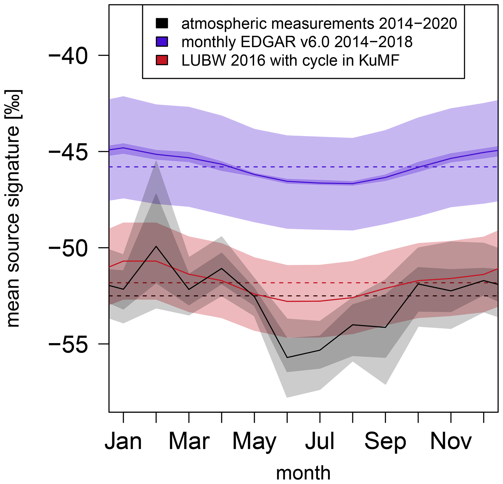
Figure 9 Annual variability in the monthly mean CH₄ isotopic source signatures calculated with emission inventories and atmospheric measurements for the Heidelberg area. The light-blue and red areas for EDGAR v6.0 (Crippa et al., 2021) and LUBW (LUBW, 2016) correspond to errors in the applied source signatures, and the dark-blue area for EDGAR v6.0 shows differences in the CH₄ isotopic source signatures for all years between 2014 and 2018. The dark-grey area corresponds to the results for atmospheric measurements from the different approaches, and the light-grey area includes errors.

The monthly mean isotopic source signatures calculated using the EDGAR v6.0 and the LUBW inventories also show an annual cycle with more depleted values in summer compared to winter. However, the peak-to-peak amplitude in the annual cycle determined out of atmospheric measurements is 5.8 ‰ and thus approximately 3 times larger than the annual cycles noticeable by EDGAR v6.0 and the modelled LUBW data. Thus, the observed annual cycle resulting from atmospheric measurements can only be partly explained by seasonal variations of CH₄ emissions from heating. This indicates that emissions from another sector have relevant seasonal variations too, which are not yet included into EDGAR v6.0 inventory.

By using inverse models, Bergamaschi et al. (2018) found an annual cycle in CH₄ emissions in Germany, with the maximum in summer. Due to the limited number of studies, they could not quantitatively estimate potential seasonal variations of anthropogenic sources (Bergamaschi et al., 2018). However, some studies such as Ulyatt et al. (2010), Spokas et al. (2011), and VanderZaag et al. (2014) reported an annual cycle in CH₄ emissions from biogenic sources such as dairy cows, landfills, or waste water with more emissions in summer. Such seasonal variations in biogenic emissions, in addition to the variations of emissions from heating, can explain the annual cycle in the catchment area of Heidelberg determined by atmospheric measurements.

The comparison between the isotopic carbon signatures determined using emissions from the EDGAR v6.0 inventory and the results from atmospheric measurements indicates that EDGAR v6.0 seems to overestimate CH₄ emissions from less depleted sources in the catchment area of Heidelberg. A recent study with mobile CH₄ measurements in Heidelberg by Wietzel and Schmidt (2023) shows that the EDGAR 6.0 and the LUBW emission inventories most probably overestimate the emissions from natural gas distribution systems in the city of Heidelberg. When comparing our results with studies in other cities, it becomes clear that the representativeness of emissions inventories can strongly vary by region and city. Saboya et al. (2022) showed that the mean isotopic source signature in EDGAR v4.3.2 for London is approximately −12 ‰ lower than the median of the isotopic source signatures, indicating that emissions due to natural gas leaks in London are being underestimated. Menoud et al. (2021) found that the average isotopic source signatures from the model using the EDGAR v5.0 inventory in Kraków are in good agreement with the ones from the measurements. These differences in the studies show the importance and significance of regional and local studies using continuous isotope measurements.

4 Conclusions

In this study, a continuous time series of atmospheric CH₄ and δ(¹³CH₄) measured over 6 years in Heidelberg is used to study seasonal variations and trends of CH₄ emissions in the catchment area of Heidelberg. The partitioning of local and regional CH₄ emissions among different source categories is analysed by determining the mean isotopic carbon source signature in the catchment area of Heidelberg. Therefore, the Keeling plot method in combination with the York fit is applied to the measured atmospheric CH₄ and δ(¹³CH₄) time series. Three different approaches are tested which correspond to different time intervals: the monthly approach, the night-time approach, and the moving Keeling plot approach. The mean isotopic carbon source signatures determined for the catchment area of Heidelberg from atmospheric measurements are then used to verify the CH₄ emissions reported by two emission inventories: EDGAR v6.0 and LUBW inventory.

No significant trend occurs during the 6 years in the monthly mean source signatures determined with all three approaches from atmospheric measurements. This was different in the 1990s, when the composition of CH₄ emissions in the Heidelberg catchment area changed due to a decline in CH₄ emissions from fossil sources (mainly coal mining) and from livestock farming (Levin et al., 1999). The average mean isotopic carbon source signature calculated with the night-time and the moving Keeling plot approaches is (−52.3 ± 0.4) ‰ in the Heidelberg catchment area. This shows that the CH₄ emissions in Heidelberg are not dominated by one source category but originate from different sources in the urban area as well as in the rural surroundings. They range from biogenic sources (livestock and waste treatment), to thermogenic sources (natural gas), and even to pyrogenic ones (traffic and wood-firing installations). This is different to previous studies, which determined the mean isotopic carbon source signatures for more rural areas in the Netherlands (Röckmann et al., 2016; Menoud et al., 2020), with strong biogenic emissions from dairy cows, or urban areas in Poland (Menoud et al., 2021) and the UK (Saboya et al., 2022), with stronger influence of fossil emissions. The LUBW inventory represents the composition of CH₄ emission well, but EDGAR v6.0 overestimates CH₄ emissions from less depleted sources, especially from waste incineration and the energy for the buildings sector. The comparison of our results with studies in other cities shows that the representativeness of emission inventories can vary greatly depending on the region and city. This demonstrates the importance and significance of regional and local studies using continuous isotope measurements.

The determined monthly mean isotopic carbon source signatures derived from atmospheric measurements show an annual cycle with a peak-to-peak amplitude of 5.8 ‰ and less depleted values in summer than in winter. Comparison with emission inventories shows that this cycle can only be partly explained by seasonal variations in the CH₄ emissions from heating and that strong seasonal variations in biogenic CH₄ emissions (waste water, landfills, or dairy cows) must contribute with stronger emissions in summer. Such an annual cycle in biogenic CH₄ emissions is not included in the monthly emissions from the EDGAR v6.0 inventory. There is thus a great need for research, to accurately understand and quantify annual cycles of CH₄ emissions. The composition of CH₄ emissions determined directly from long-term atmospheric δ(¹³CH₄) measurements, as in this study, can make a contribution to this, especially with regard to the ongoing improvement of measurement technology, and determine the annual cycle of entire source categories of a region independently of measurements at individual sources.

Our study provides an optimised method to detect the isotopic carbon source signature and its seasonal cycle of different CH₄ emitters. These provide valuable insights into the temporal resolution of CH₄ emissions on a regional scale and show how additional in situ δ(¹³CH₄) measurements could improve CH₄ emissions inventories. In particular, the ability to distinguish between over- and underestimated emission sectors in the inventories can lead to a significant improvement of high-resolution emission inventories in both temporal and spatial resolution. This study demonstrates the importance of in situ δ(¹³CH₄) long-term measurements, not only for global and regional model studies but also as a complementary tool to better understand and describe seasonal cycles in emissions, and it can be a model for other stations.

Appendix A

Table A1 CH₄ mole fraction and isotopic ratio of the two calibration gases used to calibrate the ambient air measurements carried out in Heidelberg.

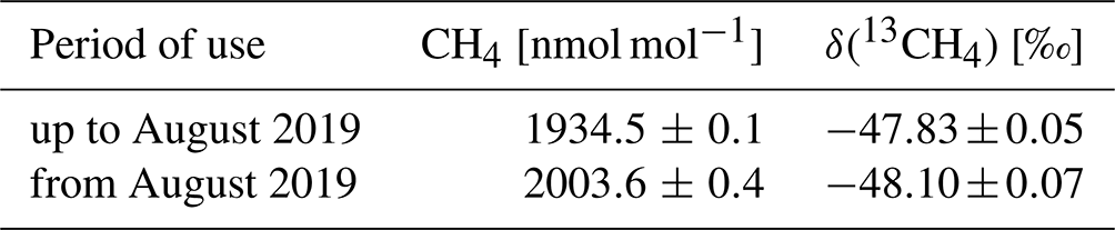
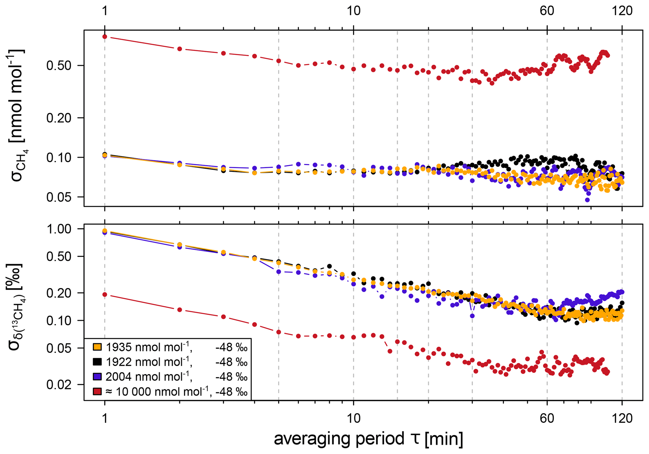
Figure A1 Allan standard deviations for CH₄ mole fraction and δ(¹³CH₄) determined for the CRDS G2201-i analyser and different CH₄ mole fractions and isotope ratios. The Allan standard deviations are based on measurements from 2013 (orange) and 2019 (black, blue, red).

Table A2 δ(¹³CH₄) measurements of six intercomparison cylinders. The δ(¹³CH₄) values determined by MPI-BGC are taken from Umezawa et al. (2018) and are compared with our results. The difference of the multiple measurements is shown in parentheses, and the uncertainty of the average difference is given as the standard error of the mean.

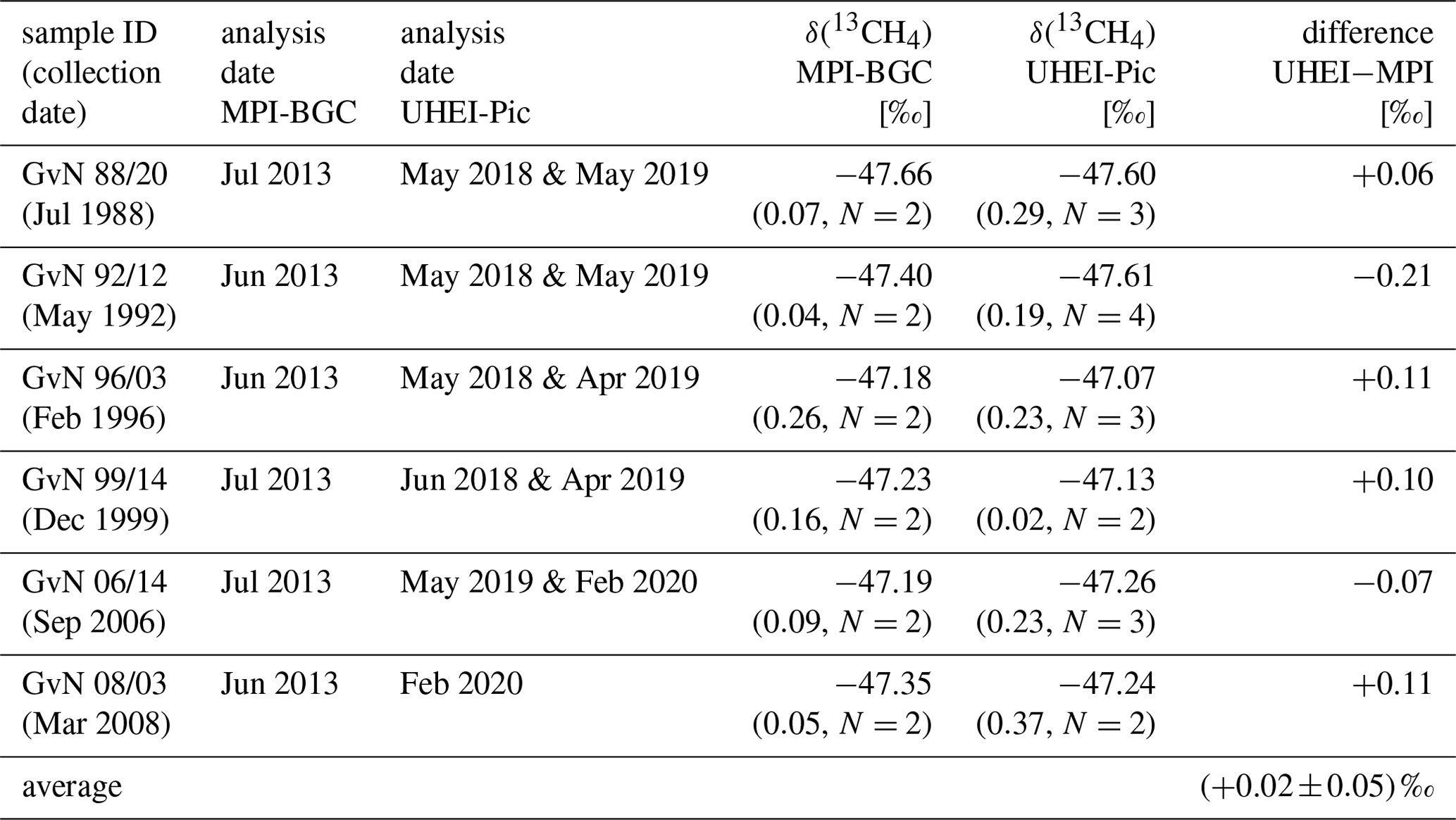
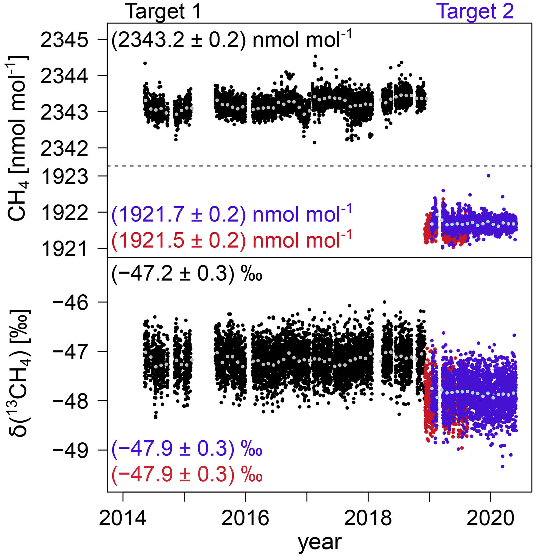
Figure A2 Calibrated CH₄ mole fractions and δ(¹³CH₄) values of the target cylinder measurements. Target 1 (calibrated with calibration cylinder 1) is shown in black and Target 2 (calibrated with calibration cylinder 2) in blue. The grey and light-blue data points correspond to the monthly average values. For quality control, Target 2 was additionally calibrated with calibration cylinder 1 and is shown here in red.