Daytime variation in the aerosol indirect effect for warm marine boundary layer clouds in the eastern North Atlantic

Warm boundary layer clouds in the eastern North Atlantic region exhibit significant diurnal variations in cloud properties. However, the diurnal cycle of the aerosol indirect effect (AIE) for these clouds remains poorly understood. This study takes advantage of recent advancements in the spatial resolution of geostationary satellites to explore the daytime variation in the AIE by estimating the cloud susceptibilities to changes in cloud droplet number concentration (N_d). Cloud retrievals for the month of July over 4 years (2018–2021) from the Spinning Enhanced Visible and Infrared Imager (SEVIRI) on Meteosat-11 over this region are analyzed. Our results reveal a significant “U-shaped” daytime cycle in susceptibilities of the cloud liquid water path (LWP), cloud albedo, and cloud fraction. Clouds are found to be more susceptible to N_d perturbations at noon and less susceptible in the morning and evening. The magnitude and sign of cloud susceptibilities depend heavily on the cloud state defined by cloud LWP and precipitation conditions. Non-precipitating thin clouds account for 44 % of all warm boundary layer clouds in July, and they contribute the most to the observed daytime variation. Non-precipitating thick clouds are the least frequent cloud state (10 %), and they exhibit more negative LWP and albedo susceptibilities compared to thin clouds. Precipitating clouds are the dominant cloud state (46 %), but their cloud susceptibilities show minimal variation throughout the day.

We find evidence that the daytime variation in LWP and albedo susceptibilities for non-precipitating clouds is influenced by a combination of the diurnal transition between non-precipitating thick and thin clouds and the “lagged” cloud responses to N_d perturbations. The daytime variation in cloud fraction susceptibility for non-precipitating thick clouds can be attributed to the daytime variation in cloud morphology (e.g., overcast or broken). The dissipation and development of clouds do not adequately explain the observed variation in cloud susceptibilities. Additionally, daytime variation in cloud susceptibility is primarily driven by variation in the intensity of cloud response rather than the frequency of occurrence of cloud states. Our results imply that polar-orbiting satellites with an overpass time at 13:30 LT underestimate daytime mean values of cloud susceptibility, as they observe susceptibility daily minima in the study region.

1 Introduction

Warm boundary layer clouds, including stratus, stratocumulus, and cumulus clouds, are prevalent over the sub-tropical oceans and account for over 30 % of the global annual mean cloud coverage (Warren et al., 1988; Wood, 2012). These clouds cause a significant net negative radiative forcing on the surface radiation budget. However, our understanding of the aerosol indirect effect (AIE) on these clouds, particularly the impact of aerosols on cloud amount, brightness, and lifetime, remains a significant source of uncertainty in estimating the radiative forcing from human activities. The AIE plays a critical role in the Earth's radiation budget through its interactions with clouds. It consists of two effects: the Twomey effect, which involves an increase in the cloud droplet number from increasing aerosols and leads to an increase in cloud albedo (α_c) from smaller droplets when the cloud liquid water path (LWP) is held constant (Twomey, 1977), and the cloud adjustment effect, which encompasses the impact of aerosols on cloud amount, cloud water, and α_c through modulating cloud processes (e.g., Albrecht, 1989; Xue and Feingold, 2006; Chen et al., 2014; Gryspeerdt et al., 2019). The cloud adjustment effect is highly variable with large uncertainties in signs and magnitudes depending on the cloud state, boundary layer, and meteorological conditions among other factors (e.g., Han et al., 2002; Wang et al., 2003; Small et al., 2009; Sato et al., 2018).

Previous studies have made significant progress in identifying different cloud processes and feedback mechanisms to explain the responses of the cloud fraction (CF), LWP, and α_c to aerosol perturbations (e.g., as summarized in Stevens and Feingold, 2009; Fan et al., 2016; Gryspeerdt et al., 2019). The cloud adjustment effect is influenced by two key feedback mechanisms: precipitation suppression and sedimentation–evaporation–entrainment.

Under clean conditions and for predominantly precipitating clouds, an increase in the cloud droplet number concentration (N_d) and an associated decrease in droplet sizes reduce precipitation efficiency and decrease water loss from precipitation. Consequently, this promotes an increase in cloudiness and cloud LWP (Albrecht, 1989; Qian et al., 2009; Li et al., 2011; Terai et al., 2012, 2015). For non-precipitating clouds, decreased cloud drop size due to increases in N_d impacts CF and LWP through their impact on the entrainment rate. A decrease in cloud droplet size diminishes the sedimentation rate in clouds, causing an accumulation of cloud water near the cloud top. This increased cloud water in the entrainment zone enhances cloud-top radiative cooling, the entrainment rate, and evaporation, resulting in a decrease in CF and cloud LWP (Bretherton et al., 2007; Chen et al., 2014; Toll et al., 2019; Gryspeerdt et al., 2019).

Additionally, the faster evaporation rates from smaller droplets enhance cloud-top cooling, downward motion in clouds, total kinetic energy, and the horizontal buoyancy gradient. The processes listed above, in turn, increase evaporation and the entrainment rate and, thus, form a positive feedback loop (Wang et al., 2003; Xue and Feingold, 2006; Small et al., 2009; Toll et al., 2019). Furthermore, among non-precipitating clouds, thick clouds with larger LWP exhibit stronger cloud-top longwave radiative cooling rates and therefore stronger cloud-top entrainment rates (e.g., Sandu et al., 2008; Williams and Igel, 2021). Therefore, the classification of cloud states (e.g., precipitating conditions and thickness) is essential for accurately quantifying the AIE and discerning opposing cloud processes. In this study, we classify cloud states based on the LWP–N_d parameter space, as these variables provide the most informative metrics for cloud susceptibility (Zhang et al., 2022).

This study focuses on the eastern North Atlantic (ENA) region, where the US Department of Energy (DOE) Atmospheric Radiation Measurement (ARM) program has deployed a ground-based user facility in the Azores archipelago (Mather and Voyles, 2013). During the summer over the ENA region, warm boundary layer clouds exhibit pronounced diurnal variations in their properties and cloud states. For example, based on ARM surface radar and lidar observations, the frequency of stratocumulus clouds is highest at night, accompanied by an increase in the fraction of precipitating clouds. Throughout the daytime, both the cloud fraction and the precipitation fraction experience a slight decrease, followed by an increase after sunset (Rémillard et al., 2012). The retrieved cloud microphysical properties from ARM ground-based observations show similar “U-shaped” diurnal variations in cloud LWP, liquid water content, and optical thickness (Dong et al., 2014). Additionally, numerical studies have revealed a distinct diurnal cycle of the AIE for marine stratocumulus clouds, attributed to changes in cloud properties and boundary layer thermodynamic conditions (e.g., Sandu et al., 2008, 2009). However, observational analyses based on the ground-based observations at the ENA site or in situ measurements from field campaigns are often based on a few cases with limited samples and insufficient spatial coverage (e.g., Liu et al., 2016; Wang et al., 2020; Zheng et al., 2022). There have been few observational studies investigating the diurnal cycle of the AIE in the ENA region. With recent advancements in the spatial resolution of geostationary satellites, this study aims to investigate the diurnal variation in the AIE in warm boundary layer clouds over the ENA region and give a better understanding of the underlying mechanisms.

Both cloud properties and meteorological conditions have substantial spatiotemporal variability and distinct diurnal variations. Furthermore, changes in meteorological conditions can in turn influence cloud and aerosol properties. One of the main challenges in understanding the AIE lies in isolating the impacts of the confounding meteorological drivers on clouds and aerosols from the AIE on clouds. To address this challenge, Gryspeerdt et al. (2016) proposed the use of N_d as an intermediary variable for the AIE, instead of using aerosol optical depth (AOD) or the aerosol index. The use of N_d circumvents the well-known dependency of AOD on CF and surface wind speed, which do not necessarily reflect actual changes in aerosol loading. Moreover, the control of relative humidity and aerosol type on AOD prevents the establishment of a direct link between AOD and aerosol concentration or cloud condensation nuclei (CCN).

Another common method to disentangle meteorological impacts is to sort the controlling meteorological factors of the cloud state, such as relative humidity, lower-tropospheric stability, or vertical velocity, and examine the AIE accordingly (e.g., Chen et al., 2014; Gryspeerdt et al., 2019). However, this approach overlooks important information, including the frequency of occurrence of specific environmental conditions, the spatiotemporal co-variation in meteorological factors, and the correlations among them. Zhou et al. (2021) and Zhang et al. (2022) proposed a new method to estimate the cloud susceptibility within a confined space (e.g., a 1° × 1° or 2° × 2° grid box) of each satellite snapshot by assuming consistent meteorological conditions within this spatial domain. Additionally, it is important to note that meteorological conditions influence albedo susceptibility by altering the frequency of occurrence of different cloud states (e.g., precipitating and non-precipitating). Specifically, within a particular cloud state, meteorological conditions offer limited information regarding cloud susceptibility (Zhang et al., 2022).

The second main source of uncertainty in observational AIE studies arises from inferring processes in a temporally evolving system based on snapshots of observations (Mülmenstädt and Feingold, 2018). Due to the limited temporal or spatial resolution of the observations, most studies assume a Markovian system, where clouds and the AIE are assumed to only relate to the current state of the system and have no memory of the past states. However, this assumption contradicts the nature of the cloud system. Observational and modeling studies have shown that aerosol–cloud interaction processes take hours to reach the equilibrium state and that the sensitivity of the AIE is time dependent. For instance, Glassmeier et al. (2021) utilized a Gaussian-process emulation and derived the adjustment equilibration timescale for LWP to be ∼ 20 h. By tracking the ship tracks in satellite observations, Gryspeerdt et al. (2021) found a similar AIE timescale of ∼ 20 h or longer and the magnitude of LWP susceptibility to increase with time. In addition, Christensen et al. (2020) discovered that the influence of aerosols on cloud LWP, CF, and cloud-top height persists for 2 to 3 d by tracking cloud systems in satellite observations. In summary, the sensitivity of cloud responses to N_d perturbations changes with time, and, thus, the assumption that the AIE has no memory of its past state is inadequate. Nonetheless, the direct evaluation of the impact of cloud memory on the quantified cloud susceptibility remains unexplored to the best of our knowledge.

To facilitate a process-level understanding of the drivers behind the diurnal variation in the AIE for warm boundary layer clouds, we will classify these clouds into three states: precipitating clouds, non-precipitating thick clouds, and non-precipitating thin clouds. We investigate the changes in both the frequency of occurrence of cloud states and the magnitude of the AIE for different cloud states throughout the day. Additionally, we document the temporal changes in cloud state within each fixed 1° × 1° grid box and quantify the influences of cloud memory and state transition on the AIE. Section 2 describes the datasets as well as the methodology employed to quantify cloud susceptibilities, distinguish precipitating clouds from the satellite retrievals, and track cloud states. We present our results in Sect. 3. Section 3.1 characterizes the general conditions of warm boundary clouds over the ENA region during the summer. Section 3.2 introduces the LWP–N_d parameter space and illustrates the dependence of cloud responses to N_d perturbations on cloud states. We then discuss the mean daytime variation in cloud susceptibilities for all cloud states in Sect. 3.3, followed by an analysis of the AIE daytime variation for each cloud state and the impact of the state transition on the AIE in Sect. 3.4. In Sect. 3.5, we decompose the contributions to the daytime variation in cloud susceptibility into two components: one is from changes in the frequency of occurrence of different cloud states, and the other is from changes in the intensity of the AIE during the day. Section 4 includes discussions on the similarities and differences in findings between this study and previous studies of the AIE, and Sect. 5 gives the summary and conclusions of this study.

2 Dataset and methodology

We use cloud retrievals derived from the Spinning Enhanced Visible and Infrared Imager (SEVIRI) on Meteosat-11, with a spatial resolution of 3 km at nadir and a half-hourly temporal resolution over the ENA region (33–43° N, 23–33° W). SEVIRI cloud products are derived using the Satellite ClOud and Radiation Property retrieval System (SatCORPS) algorithms (e.g., Painemal et al., 2021), based on the methods applied by the Clouds and the Earth's Radiant Energy System (CERES) project and specifically tailored to support the ARM program over the ARM ground-based observation sites (Minnis et al., 2011, 2020). Given the purpose of this study to quantify the AIE on warm boundary layer clouds, we focus on July over 4 years (2018–2021), a period that coincides with the highest frequency of occurrence of warm boundary layer clouds over the ARM ENA site (Rémillard et al., 2012; Dong et al., 2014, 2023).

The cloud mask algorithm implemented in SatCORPS is described in Trepte et al. (2019). SatCORPS cloud properties are based on the shortwave-infrared split-window technique during the daytime (VISST; Minnis et al., 2011, 2020), with the cloud optical depth (τ) and effective radius (r_e) being derived using an iterative process that combines reflectance and brightness temperatures from the 0.64 and 3.9 µm channels. Cloud LWP is computed from τ and r_e using the formula $\mathrm{LWP}=\frac{\mathrm{4}{r}_{\mathrm{e}}\mathit{\tau }}{\mathrm{3}{Q}_{\text{ext}}}$, where Q_ext represents the extinction efficiency and assumed constant of 2.0 (Minnis et al., 2011, 2020). The top-of-atmosphere (TOA) broadband shortwave α_c is derived from an empirical radiance-to-broadband conversion using the satellite imager's visible channel and CERES Single Scanner Footprint (SSF) shortwave fluxes and dependent on the solar zenith angle and surface type (Minnis et al., 2016). Cloud-top height computation follows the methodology in Sun-Mack et al. (2014).

To validate the Meteosat-11-retrieved cloud mask and the detection of boundary layer clouds, we compare the boundary layer cloud fractions derived from Meteosat-11 with the ground-based observations at the ARM ENA site. As seen in Fig. S1 in the Supplement, both the diurnal variation and the mean CF of Meteosat-11 agree well with ARM observations. More details on the methodology for the evaluation study are included in the Supplement.

Our analysis focuses on warm boundary layer clouds with cloud tops below 3 km and a liquid cloud phase. To focus specifically on boundary layer cloud cases without including the edges of deep clouds, we apply a stricter threshold than merely using the pixel-level cloud-top height. We define boundary layer clouds as those with 90 % of their cloud tops below 3 km, labeling all contiguous cloudy pixels as distinct cloud objects.

Cloud N_d is retrieved based on the adiabatic assumptions for warm boundary layer clouds, as in Grosvenor et al. (2018), according to the following equation:

$$\begin{array}{}\text{(1)}& N_{\mathrm{d}}={\displaystyle \frac{\sqrt{\mathrm{5}}}{\mathrm{2}\mathit{\pi }k}}{\left({\displaystyle \frac{f_{\text{ad}}{c}_{\mathrm{w}}\mathit{\tau }}{Q_{\text{ext}}{\mathit{\rho }}_{\mathrm{w}}{r}_{\mathrm{e}}^{\mathrm{5}}}}\right)}^{\mathrm{1}/\mathrm{2}}.\end{array}$$

In Eq. (1), k represents the ratio between the volume mean radius and r_e, assumed to be constant at 0.8 for stratocumulus; f_ad is the adiabatic fraction of the observed liquid water path and is assumed to be 0.8 for stratocumulus clouds (Brenguier et al., 2011; Zuidema et al., 2012); c_w is the condensation rate, which is a function of temperature and pressure; Q_ext is the extinction coefficient, approximated as 2 in this study; and ρ_w is the density of liquid water. While the different components of Eq. (1) could contribute to the uncertainties in N_d, errors in r_e are the dominant drivers in Eq. (1) (Grosvenor et al., 2018).

To minimize uncertainties associated with bias in satellite cloud microphysical retrievals, we only select pixels with a minimum r_e of 3 µm, a minimum τ of 3, and a solar zenith angle (SZA) of less than 65° (e.g., Painemal et al., 2013; Painemal, 2018; Zhang et al., 2022). The SZA threshold of 65° was chosen to minimize biases observed at high solar zenith angles in r_e and τ (e.g., Grosvenor and Wood, 2014; Grosvenor et al., 2018).

In addition, to reduce uncertainties associated with the adiabatic assumption in the N_d retrieval, we implement a filtering process. For each cloud, we exclude cloudy pixels at the cloud edge, defined as those adjacent to cloud-free pixels, following a similar sampling strategy to that suggested by Gryspeerdt et al. (2022). Therefore, all cloud properties in this study refer to the properties of the cloud body without the cloud edge. It is worth noting that shallow cumulus clouds with diameters smaller than 9 km are not included. The removal of cloud-edge pixels accounts for ∼ 14 % of the cloudy pixels. Furthermore, we removed grid boxes containing islands due to the uncertainties in Meteosat retrievals over contrasting underlying surfaces. Lastly, to avoid unrealistically large retrievals, we eliminate pixels with the retrieved N_d values exceeding 1000 cm⁻³, which constituted only 0.002 % of the data.

Cloud susceptibility is quantified as the slope between cloud properties and N_d using a least-squares regression. As found by Arola et al. (2022) and Zhou and Feingold (2023), the retrieved cloud susceptibilities are sensitive to small-scale cloud heterogeneity, the co-variability between cloud properties and N_d, and the spatial scale of cloud organization. To reduce biases resulting from heterogeneity and co-variability, we first average the 3 km pixel-level cloud retrievals and N_d (Eq. 1) to a regular 0.25° × 0.25° grid for each half-hourly time step.

To further mitigate the impact from co-variability between cloud properties and N_d at larger spatiotemporal scales, cloud susceptibility is estimated within a 1° × 1° grid box at each satellite time step (e.g., Zhang et al., 2022). Moreover, estimating the cloud susceptibility over a confined space also helps to constrain the meteorological impacts on the AIE, with the assumption of a homogeneous meteorological condition within this spatial scale. Next, susceptibilities are calculated using the 0.25° smoothed data if the number of data points within the 1° × 1° box exceeds 6 (from a maximum of 16 data points). It is important to note that when computing the 0.25° × 0.25° averaged cloud properties, only data from cloudy pixels are used to ensure that the estimated susceptibility is not weighted by CF or impacted by satellite artifacts. Lastly, due to the minimal spatial variability in cloud susceptibility in the study region, the 1° cloud susceptibility is averaged over the study region (33–43° N, 23–33° W) to characterize the daytime variation in the AIE. Additionally, the results and conclusions of this study are not sensitive to the size of the box used in calculating the cloud susceptibility (e.g., over a 0.8° × 0.8° box or over a 1.5° × 1.5° box, not shown).

Because of the nonlinear relationships between LWP and N_d, the LWP susceptibility is defined as the slope in logarithmic scale, that is $\mathrm{d}\text{ln}\left(\mathrm{LWP}\right)/\mathrm{d}\text{ln}(N_{\mathrm{d}}$) (e.g., Gryspeerdt et al., 2019). The albedo susceptibility is estimated as the slope between α_c and ln(N_d), equivalent to $\mathrm{d}{\mathit{\alpha }}_{\mathrm{c}}/\mathrm{d}\text{ln}(N_{\mathrm{d}}$) (e.g., Painemal, 2018). Lastly, the CF susceptibility is estimated as $\mathrm{d}\mathrm{CF}/\mathrm{d}\text{ln}(N_{\mathrm{d}}$). The mean CF is defined as the cloudy pixels excluding the cloud edge as a fraction of the sum of cloudy and clear pixels within each 0.25° × 0.25° box. Due to the highly variable nature of CF, the variability in the 0.25° CF could arise from quantifying edges or centers of the same cloud layer rather than N_d perturbations. To assess the potential influence of cloud morphology on the retrieved CF susceptibility, we did a sensitivity test to exclude any 1° × 1° scene meeting the following three criteria: (1) the difference between the maximum and minimum 0.25° CF is greater than 0.9, (2) the variation in the 0.25° N_d is less than 60 cm⁻³, and (3) the 0.25° CF in the 1° × 1° box samples the same cloud. The 0.9 and 60 cm⁻³ thresholds represent ∼ 45 % of the data. With the three thresholds combined, a total of 17 000 scenes were removed, which accounts for ∼ 24 % of the total samples. Removing these scenes does not change the conclusions of CF susceptibility in this study (not shown), which demonstrates that cloud morphology has minimal impact on the retrieved CF susceptibility. Furthermore, as we removed N_d retrievals at the cloud edge where N_d likely suffers large uncertainties, cloudy pixels at the cloud edge are set as clear for consistency in the calculation of the CF susceptibility. Removing the cloud edge decreases the 4-month mean CF for warm boundary layer clouds from 21.6 % to 19.0 %.

The susceptibility of the shortwave radiative fluxes to N_d (F₀) is estimated as the sensitivity of the TOA shortwave upward radiative flux (${\mathrm{SW}}_{\mathrm{TOA}}^{\mathrm{up}}$) to N_d perturbations (e.g., Chen et al., 2014; Painemal, 2018; Zhang et al., 2022). The mean ${\mathrm{SW}}_{\mathrm{TOA}}^{\mathrm{up}}$ over a 1° × 1° grid box is estimated using Eq. (2), with the assumption that the clear-sky albedo over the ocean is small compared to the cloud albedo:

$$\begin{array}{}\text{(2)}& \stackrel{\mathrm{‾}}{{\mathrm{SW}}_{\mathrm{TOA}}^{\mathrm{up}}}=\stackrel{\mathrm{‾}}{{\mathrm{SW}}_{\mathrm{TOA}}^{\mathrm{dn}}}\cdot \stackrel{\mathrm{‾}}{{\mathit{\alpha }}_{\mathrm{c}}}\cdot \stackrel{\mathrm{‾}}{\mathrm{CF}},\end{array}$$

where ${\mathrm{SW}}_{\mathrm{TOA}}^{\mathrm{dn}}$ is the grid-box mean TOA shortwave downward radiative flux, which is estimated based on the latitude, longitude, date, and overpass time of each pixel, and α_c and CF are the grid-box mean values. Then, F₀ is estimated using the calculated α_c and CF susceptibilities and the 1° × 1° grid-box mean cloud properties as shown in the equation below:

$$\begin{array}{}\text{(3)}& \begin{array}{rl}{F}_{\mathrm{0}}& =-{\displaystyle \frac{\mathrm{d}{\mathrm{SW}}_{\mathrm{TOA}}^{\mathrm{up}}}{\mathrm{d}\text{ln}\left(N_{\mathrm{d}}\right)}}\\ & =-\stackrel{\mathrm{‾}}{{\mathrm{SW}}_{\mathrm{TOA}}^{\mathrm{dn}}}\cdot \left({\displaystyle \frac{\mathrm{d}{\mathit{\alpha }}_{\mathrm{c}}}{\mathrm{d}\text{ln}\left(N_{\mathrm{d}}\right)}}\cdot \stackrel{\mathrm{‾}}{\mathrm{CF}}+{\displaystyle \frac{\mathrm{d}\mathrm{CF}}{\mathrm{d}\text{ln}\left(N_{\mathrm{d}}\right)}}\cdot \stackrel{\mathrm{‾}}{{\mathit{\alpha }}_{\mathrm{c}}}\right).\end{array}\end{array}$$

F₀ is in units of $\mathrm{W}{\mathrm{m}}^{-\mathrm{2}}\text{ln}(N_{\mathrm{d}}{)}^{-\mathrm{1}}$, and a positive value indicates a decrease in the ${\mathrm{SW}}_{\mathrm{TOA}}^{\mathrm{up}}$, which is a warming effect at the surface.

To minimize uncertainties in the linear regression for the estimated susceptibility, we analyze regressions that exhibited a goodness of fit exceeding the 95 % confidence interval (i.e., ${\mathit{\chi }}^{\mathrm{2}}<{\mathit{\chi }}_{\mathrm{0.95},\mathrm{c}}^{\mathrm{2}}$) and an absolute correlation coefficient greater than 0.2 (e.g., Painemal, 2018; Zhang et al., 2022). There are a total of ∼ 115 000 samples of the 1° cloud susceptibilities in this study; applying the goodness-of-fit thresholds results in exclusions of ∼ 33 000–43 000 samples for different susceptibilities, which comprise ∼ 28 %–37 % of the data. Sensitivity test shows that including cases that fail the goodness-of-fit test will not change the results and conclusions of this study (not shown). Specifically, including these cases decreases the magnitude of cloud susceptibilities for all three cloud states, but the signs of cloud responses to N_d perturbations remain consistent.

Since precipitating and non-precipitating clouds exhibit distinct responses to aerosol perturbations due to the effect of precipitation suppression and the wet-scavenging feedback, it is critical to distinguish between these two cloud states when estimating the AIE. Previous studies have utilized various methods based on the effective radius threshold (e.g., Gryspeerdt et al., 2019; Toll et al., 2019; Zhang et al., 2022) and the rain rate threshold (e.g., Duong et al., 2011; Terai et al., 2015) from satellite retrievals. In our study, we validate these two methods using the precipitating mask estimated from ground-based observations with a radar reflectivity threshold together with the lidar-defined cloud base at the ARM ENA site (e.g., Wu et al., 2020a). The thresholds of r_e > 12 µm and r_e > 15 µm yield hit rates of 0.79 and 0.73, respectively. However, the false alarm rate is higher for r_e > 12 µm (0.21) compared to r_e > 15 µm (0.1). The rain rate is computed using the empirical relationships derived from ground-based measurements in Comstock et al. (2004) as $R=\mathrm{0.0156}(\mathrm{LWP}/N_{\mathrm{d}}{)}^{\mathrm{1.75}}$. Using a threshold of R > 0.05 mm h⁻¹ results in a hit rate of 0.65. Consequently, we use the r_e > 15 µm threshold to define precipitating clouds in this study.

To investigate the dependencies of cloud susceptibility on previous cloud states and quantify the influence of cloud memory on the estimated cloud susceptibility, we track the historical cloud state over a 1° × 1° grid box for a 2 h period. During the summer in the study region, low-wind conditions prevail in the boundary layer, with the mean wind speed being less than 10 m s⁻¹ for 85 % of the time and less than 7 m s⁻¹ for 60 % of the time. Therefore, in most cases, fewer than half of the clouds exit the grid box within the 2 h, allowing us to track the previous cloud state within the same grid box (i.e., from the Eulerian perspective). The influence of cloud memory is assessed by comparing the cloud susceptibilities of clouds that undergo a transition in cloud state with those that do not experience such a transition. Section 3.4 provides more details and discussion on the sensitivity of tracking time and the influence of advection on our classification.

3 Results

3.1 General cloud conditions and mean cloud responses to N_d perturbations

In the ENA region, characterized by the dominant Bermuda High with its prevailing ridge and zonal synoptic pattern (Mechem et al., 2018), the summer season gives rise to the annual peak in boundary layer cloud coverage. The monthly mean low-level CF retrieved from Meteosat-11 reaches its maximum of 35 % in July, compared to an annual mean of 17 % during the 4-year study period. This region represents a typical clean marine condition, situated far from continental influences, which results in a consistently low N_d compared to polluted marine regions, such as the northeastern (NE) Pacific near California or the northwestern Atlantic near the Gulf of Maine. In July, the mean N_d over the ENA region is 65 cm⁻³ with lower 5th and upper 95th percentiles of 15 and 160 cm⁻³, respectively. The retrieved N_d values in this study closely align with in situ measurements from the Aerosol and Cloud Experiments in Eastern North Atlantic (ACE-ENA) field campaign. For instance, the in situ-measured N_d in July 2017 varied from 25 to 150 cm⁻³, with a mean value of 65 cm⁻³ (e.g., Yeom et al., 2021; Zhang et al., 2021). Moreover, our satellite-retrieved N_d exhibits good agreement with retrievals based on ground-based observations at the ARM ENA site (e.g., Dong et al., 2014; Wu et al., 2020b) and the Moderate Resolution Imaging Spectroradiometer (MODIS; e.g., Bennartz, 2007; Bennartz and Rausch, 2017).

Figure 1 Relationships between N_d and cloud properties: (a) cloud LWP, (b) cloud albedo, (c) cloud fraction, and (d) TOA shortwave upward radiative flux. The dots represent the mean values, while the whiskers indicate the upper and lower 25th percentiles. In (a), the dashed line denotes r_e = 15 µm, serving as an indicator of precipitation occurrence, with precipitating clouds located to the left of the line. Light-blue, green, and magenta lines in panels (a)–(d) represent the regression slopes of the mean cloud properties and the mean ln(N_d) for N_d < 40 cm⁻³, N_d between 40 and 80 cm⁻³, and N_d > 80 cm⁻³, respectively.

Previous studies have demonstrated that clouds exhibit diverse responses to aerosol perturbations under clean and polluted conditions (e.g., Fan et al., 2016; Mülmenstädt and Feingold, 2018). Figure 1 shows the relationships between the climate mean cloud properties, derived from the pixel-level SEVIRI cloud products and averaged to the 1° × 1° resolution, as a function of the 1° × 1° mean N_d values. To quantify these responses, cloud susceptibility is estimated as the slope of the mean cloud variable changes across N_d bins. In pristine conditions (N_d < 40 cm⁻³, ∼ 28 % of data), clouds predominantly precipitate (r_e > 15 µm, Fig. 1a). The mean cloud LWP features a slight increase followed by a decrease with increasing N_d. This result departs from the precipitation suppression hypothesis, in which LWP typically increases. The absence of a precipitation suppression signal is likely attributable to the relatively modest precipitation that occurs in this region during summer (e.g., Wu et al., 2020b; Zheng and Miller, 2022), resulting in a minimal precipitation suppression effect and a dominant entrainment drying effect. In terms of α_c, the potential decrease in α_c attributed to a LWP reduction offsets the potential increases in α_c caused by the Twomey effect, resulting in a net-zero change in mean α_c for clouds with N_d < 40 cm⁻³ (Fig. 1b). Furthermore, the majority of precipitating clouds are broken, with a mean CF that increases with N_d from 0.35 to 0.45 (Fig. 1c). Consequently, the mean ${\mathrm{SW}}_{\mathrm{TOA}}^{\mathrm{up}}$ flux increases from 100 to 140 W m⁻² as N_d increases from 10 to 40 cm⁻³. This increase in CF for precipitating clouds aligns with previous studies over the North Atlantic region across all seasons (e.g., Gryspeerdt et al., 2016). In summary, despite the slight decrease in mean LWP with increasing N_d for precipitating clouds, the mean cloud albedo remains relatively constant, while the mean CF increases, resulting in an overall increase in the TOA reflected shortwave flux.

Under relatively polluted conditions with N_d > 40 cm⁻³ (∼ 72 % of data), the mean LWP shows a decreasing trend with N_d. For N_d values between 40–80 cm⁻³, the $\text{ln}\left(\mathrm{LWP}\right)/\text{ln}\left(N_{\mathrm{d}}\right)$ slope is −0.37, while for N_d exceeding 80 cm⁻³, the slope reaches −0.26 (green and magenta lines in Fig. 1a). This negative adjustment of LWP for non-precipitating clouds is consistent with the sedimentation–evaporation–entrainment feedback, as well as with previous studies of stratocumulus clouds in other regions (e.g., Gryspeerdt et al., 2019; Zhang et al., 2022). The mean α_c remains nearly constant within the N_d range of 40–80 cm⁻³ (Fig. 1b). As LWP decreases at a slower rate for N_d > 80 cm⁻³, the Twomey effect becomes more dominant and leads to a slight increase in α_c with a slope of 0.01 (magenta line in Fig. 1b). For non-precipitating clouds, the mean CF slightly increases with increasing N_d with a CF susceptibility of 0.06 and 0.01 (green and magenta lines in Fig. 1c). As a result, the ${\mathrm{SW}}_{\mathrm{TOA}}^{\mathrm{up}}$ flux exhibits a weaker susceptibility compared to precipitating clouds (Fig. 1d).

3.2 Daytime mean cloud susceptibilities in the LWP–N_d space

One limitation of the relationships derived from the mean cloud properties with sorted N_d is the confounding effect from meteorological impacts on cloud properties and cloud susceptibilities. As a comparison, Fig. 2 shows the mean cloud susceptibility estimated within each half-hourly snapshot's 1° × 1° grid box and averaged in the LWP–N_d parameter space. There are around 72 000–82 000 samples of the 1° cloud susceptibilities in this study. The number of samples for different cloud susceptibilities are slightly different due to the goodness-of-fit test for each regression. We calculate the mean susceptibilities for LWP–N_d bins with more than 100 cloud susceptibility samples. Blank bins in Fig. 2 are bins with fewer than 100 samples. Figure 2e shows the occurrence frequency of samples for the LWP susceptibility in Fig. 2a.

Figure 2 Mean cloud susceptibilities for different N_d and LWP bins during the daytime. (a) Cloud LWP susceptibility ($\mathrm{d}\text{ln}\left(\mathrm{LWP}\right)/\mathrm{d}\text{ln}\left(N_{\mathrm{d}}\right))$, (b) cloud albedo susceptibility ($\mathrm{d}{\mathit{\alpha }}_{\mathrm{c}}/\mathrm{d}\text{ln}\left(N_{\mathrm{d}}\right))$, (c) cloud fraction susceptibility ($\mathrm{d}\mathrm{CF}/\mathrm{d}\text{ln}\left(N_{\mathrm{d}}\right))$, (d) cloud shortwave susceptibility ($-\mathrm{d}{\mathrm{SW}}_{\mathrm{TOA}}^{\mathrm{up}}/\mathrm{d}\text{ln}\left(N_{\mathrm{d}}\right))$ weighted by the frequency of occurrence of samples of each bin, and (e) frequency of occurrence of samples in each bin. The dashed lines in (a)–(e) indicate r_e = 15 µm and LWP = 75 g m⁻², as thresholds for precipitation (precipitating clouds located to the left of the line) and thick clouds (with LWP > 75 g m⁻²). The three defined cloud states are noted in (a).

With the assumption that the meteorological condition is homogeneous in each grid box, the estimated cloud susceptibilities exhibit much stronger relationships for all cloud variables compared to the climatological-mean adjustment rates shown in Fig. 1. The disparities between the two methods suggest that meteorological confounders tend to obscure the signal of the AIE over the ENA region. Moreover, the cloud responses for both precipitating and non-precipitating clouds exhibit consistent signs between the half-hourly (Fig. 2) and climatological-mean approaches (Fig. 1). This consistency is likely attributable to the confined domain (at 10° × 10°) and the focus on July in this study, which limit the spatial and temporal co-variability between cloud properties and N_d. This consistency also demonstrates that the overall cloud responses to N_d perturbations primarily depend on cloud states (e.g., precipitating conditions and cloud thickness).

The dependence of the cloud response on the cloud state is illustrated in Fig. 2. We define three cloud states: (1) the precipitating clouds (r_e > 15 µm), (2) the non-precipitating thick clouds (r_e < 15 µm, LWP > 75 g m⁻²), and (3) the non-precipitating thin clouds (r_e < 15 µm, LWP < 75 g m⁻²), which is similar to the definition in Zhang et al. (2022).

3.2.1 Precipitating clouds

Among warm boundary layer clouds, precipitating clouds are the dominant cloud state in July over the study region, with a total frequency of occurrence of 46 % (Fig. 2e). The increase in cloud LWP with increasing N_d is observed primarily in heavily precipitating thick clouds with N_d < 30 cm⁻³ and LWP > 125 g m⁻² (Fig. 2a). However, these clouds occur relatively infrequently in ENA, accounting for only 2 % of the total warm-boundary-cloud population (Fig. 2e). In contrast, most of the precipitating clouds in ENA are lightly precipitating with 15 < r_e < 20 µm (Figs. 2e and S2c in the Supplement) and they exhibit a slight decrease in LWP with N_d (Fig. 2a). The mean LWP susceptibility for lightly precipitating clouds ranges from −0.5 to −0.2 for different bins, with a mean value of −0.4. The standard deviations of LWP susceptibility in different LWP–N_d bins vary between 0.4 and 1.2, while the LWP susceptibilities for precipitating clouds are significantly different than the two other cloud states at a 95 % confidence level. The slight decrease in LWP for lightly precipitating clouds aligns with previous findings over the Pacific, Atlantic, and global oceans for marine stratocumulus (e.g., Fig. S4 in Zhang and Feingold, 2023).

The contrasting response of LWP to N_d perturbations for lightly and heavily precipitating clouds can be attributed to the interplay of two competing processes: the depletion of LWP caused by the sedimentation–evaporation–entrainment feedback and the accumulation of LWP resulting from the precipitation suppression feedback. Heavily precipitating clouds are predominantly overcast with a mean CF of 0.65 (Fig. S2a) and a mean r_e of 25 µm (Fig. S2c). Precipitation acts to stabilize the boundary layer, remove water from the cloud top, and reduce the entrainment rate (Sandu et al., 2008, 2009). Therefore, heavily precipitating clouds exhibit smaller entrainment rates than non-precipitating clouds with similar LWPs. The increase in LWP from precipitating suppression feedback outweighs the decrease in LWP from entrainment feedback and results in a net increase in LWP (e.g., Chen et al., 2014; Toll et al., 2019). In lightly precipitating clouds, however, the suppression effect of drizzle on the entrainment rate is minimal. Therefore, the decrease in LWP from entrainment overpowers the increases in LWP from precipitating suppression, leading to a net decrease in LWP with increasing N_d (e.g., Xue and Feingold, 2006).

Precipitating clouds generally exhibit brighter cloud albedo with increasing N_d as a result of the weak negative and positive LWP adjustment, particularly in heavily precipitating clouds (Fig. 2b). For lightly precipitating clouds, α_c susceptibilities range from −0.04 to 0.07 ln(N_d)⁻¹, with a mean of 0.02 ln(N_d)⁻¹. The suppression of precipitation by N_d also leads to a significant increase in CF for heavily precipitating clouds, with slopes greater than 0.25 ln(N_d)⁻¹. For most of the lightly precipitating clouds, the mean CF exhibits small variation with N_d perturbations, with CF susceptibilities in the range of ± 0.025 ln(N_d)⁻¹ (Fig. 2c). The standard deviation of the 1° α_c and CF susceptibilities for different precipitating bins ranges between 0.05–0.15 and 0.3–0.6, respectively. The α_c and CF susceptibilities for precipitating clouds are significantly different than the two other cloud states at a 95 % confidence level. Considering the combined effects of increased α_c and CF, the mean radiative response for precipitating clouds amounts to −13 $\mathrm{W}{\mathrm{m}}^{-\mathrm{2}}\ln (N_{\mathrm{d}}{)}^{-\mathrm{1}}$, which is a cumulative shortwave susceptibility of bins classified as precipitating clouds in Fig. 2d, weighted by their frequency of occurrence. The contributions from CF and α_c effects are −9.5 and −3.5 $\mathrm{W}{\mathrm{m}}^{-\mathrm{2}}\ln (N_{\mathrm{d}}{)}^{-\mathrm{1}}$, respectively (Eq. 3).

3.2.2 Non-precipitating thick clouds

Non-precipitating thick clouds are less frequent: the total frequency of occurrence is 10 % (Fig. 2e). Their cloud LWP responses to N_d perturbations differ from those of precipitating clouds. The LWP susceptibility for non-precipitating thick clouds is the most negative among the three cloud states, and it reaches a minimum value of −1.2 at the high-LWP and high-N_d ends (Fig. 2a). As LWP and N_d decrease, the LWP susceptibility gradually increases from −1.2 to −0.6. This negative susceptibility is likely explained by the evaporation enhancement associated with smaller droplets at high N_d values (e.g., Xue and Feingold, 2006; Small et al., 2009), which works in concert with an entrainment strengthening expected in clouds with large LWPs (e.g., Sandu et al., 2008; Williams and Igel, 2021). In addition, clouds with higher N_d and larger LWPs exhibit stronger shortwave absorption, which enhances LWP depletion and therefore a more negative LWP susceptibility (e.g., Boers and Mitchell, 1994; Petters et al., 2012). The mean LWP susceptibility for non-precipitating thick clouds is −0.94. Consistent with the negative LWP susceptibility, non-precipitating thick clouds become less reflective with increasing N_d for all N_d bins with LWP > 75 g m⁻² (Fig. 2b). The mean α_c susceptibility is −0.04 ln(N_d)⁻¹. Due to the enhanced entrainment and evaporation, the mean CF mostly decreases with increasing N_d, with the mean CF susceptibilities ranging from −0.1 to +0.04 ln(N_d)⁻¹ (Fig. 2c). Considering the decrease in both α_c and CF, non-precipitating thick clouds exhibit a warming effect at the surface: the mean radiative response is +4.4 $\mathrm{W}{\mathrm{m}}^{-\mathrm{2}}\ln (N_{\mathrm{d}}{)}^{-\mathrm{1}}$ (Fig. 2d), with contributions from the albedo effect and the CF effect of 2.9 and 1.5 $\mathrm{W}{\mathrm{m}}^{-\mathrm{2}}\ln (N_{\mathrm{d}}{)}^{-\mathrm{1}}$, respectively.

3.2.3 Non-precipitating thin clouds

Non-precipitating thin clouds are more common than thick clouds during summer, with a total frequency of occurrence of 44 % (Fig. 2e). Compared to non-precipitating thick clouds, they exhibit consistent negative but slightly weaker LWP responses to N_d perturbations. The mean LWP susceptibilities range from −0.9 to −0.4 in different LWP–N_d bins with a mean of −0.7 (Fig. 2a). Similarly to non-precipitating thick clouds, non-precipitating thin clouds mostly become darker with increasing N_d. Interestingly, with largely decreased LWPs, the mean CF mostly increases for all N_d conditions; the CF susceptibilities range from +0.02 to +0.25 ln(N_d)⁻¹ (Fig. 2c). The sedimentation–evaporation–entrainment feedback alone cannot explain the opposite signs in LWP and CF susceptibilities for non-precipitating thin clouds. A possible explanation for the increased CF is that the enhanced cloud-top radiative cooling rate from aerosol perturbations helps to mix the boundary layer, facilitates moisture transport from the ocean surface to clouds, and therefore favors new cloud formation and extends cloud lifetime (e.g., Christensen et al., 2020). This hypothesis is consistent with and supported by the relatively low CF for these clouds (Fig. S2a) and the diurnal variation in LWP susceptibility for non-precipitating thin clouds, which will be discussed in the next section. The opposite signs of LWP and CF susceptibilities indicate that the AIE might redistribute cloud water horizontally and make the thin clouds thinner and wider. The CF radiative effect from increased CF dominates the albedo effect from darker clouds and leads to a net cooling at the surface. The mean radiative response is −5.2 $\mathrm{W}{\mathrm{m}}^{-\mathrm{2}}\ln (N_{\mathrm{d}}{)}^{-\mathrm{1}}$, with CF and albedo contributions of −8.3 and +3.1 $\mathrm{W}{\mathrm{m}}^{-\mathrm{2}}\ln (N_{\mathrm{d}}{)}^{-\mathrm{1}}$, respectively (Fig. 2d).

To sum up, the magnitudes and signs of the responses of cloud LWP, α_c, and CF to N_d perturbations primarily depend on the cloud states. Precipitating clouds mostly become thinner and brighter with increasing N_d, accompanied by a slight increase in CF. An increase in LWP with increasing N_d is observed only for heavily precipitating clouds with N_d < 30 cm⁻³ and LWP > 125 g m⁻². Non-precipitating thick clouds become thinner and less reflective and decrease in cloudiness with N_d perturbations. On the other hand, non-precipitating thin clouds become thinner and less reflective, but their cloudiness increases as N_d increases. Given the dependence of the AIE on cloud state, we will apply the cloud state classification in the following two sections with the goal of facilitating a process-level understanding of cloud responses and the daytime variation in cloud susceptibilities.

3.3 Daytime variation in cloud susceptibility

As discussed in the Introduction, warm boundary layer clouds exhibit a distinct diurnal cycle in both cloud properties and frequency of occurrence of cloud states during summer. In this section, we investigate the daytime variation in cloud susceptibility from 09:00 to 18:00 LST (local standard time) using the half-hourly Meteosat-11 retrievals. The domain mean daytime variation in cloud susceptibility is estimated from each half-hourly time step within each 1° × 1° box and then averaged over the study domain (33–43° N, 23–33° W) during the 4 months. In the study domain, there is little spatial variability in cloud susceptibilities, and the diurnal cycle of the cloud susceptibility for the 1° × 1° box at the ARM ENA site agrees well with the domain mean pattern (not shown). Furthermore, the diurnal cycle of the cloud microphysical properties (e.g., r_e, τ, LWP, N_d) shows little difference between the domain mean value or that averaged over the 1° × 1° box at the ARM ENA site. The cloud microphysics retrievals from Meteosat-11 agree well with retrievals based on ground-based radar and lidar observations in terms of the daytime variation (not shown). Therefore, the ARM ENA site in the Azores archipelago can represent the cloud properties and the AIE for warm boundary layer clouds over the study region.

Warm boundary layer clouds witness distinct and significant daytime variations in cloud susceptibilities (Fig. 3). For example, the mean LWP susceptibility exhibits a magnitude of change of 0.4 from morning to evening, which corresponds to approximately 30 %–40 % of the overall variability in LWP susceptibility (Fig. 3a). Similarly, the α_c and CF susceptibility undergo a magnitude of changes of approximately 20 %–30 % compared to the overall variability (Fig. 3b and c). The high variability in cloud susceptibility highlights the complex synoptic, meteorological, and cloud conditions as well as the interplay between them in the ENA region. Nevertheless, the daytime variation in cloud susceptibility is statistically significant at a 95 % confidence level based on Student's t test. Interestingly, all three cloud variables exhibit a U-shaped diurnal cycle in cloud susceptibilities with less negative/more positive values in the morning and evening and more negative values at noon. Additionally, both α_c and CF susceptibilities switch signs from positive in the morning to negative at noon and then become positive again in the evening. The switch in sign for albedo susceptibility is statistically significant at a 95 % confidence level, while the switch in sign for CF susceptibility is not statistically significant (Fig. 3b and c). As both α_c and CF increase with increasing N_d in the morning, the AIE has a cooling effect at the surface, and the estimated shortwave susceptibility is −1.4 $\mathrm{W}{\mathrm{m}}^{-\mathrm{2}}\ln (N_{\mathrm{d}}{)}^{-\mathrm{1}}$. During 13:00–15:00 LST, the shortwave susceptibility switches sign to a warming effect of +1.2 $\mathrm{W}{\mathrm{m}}^{-\mathrm{2}}\ln (N_{\mathrm{d}}{)}^{-\mathrm{1}}$ (Fig. 3d).

Figure 3 Daytime variation in cloud susceptibilities. (a) Cloud LWP susceptibility ($\mathrm{d}\text{ln}\left(\mathrm{LWP}\right)/\mathrm{d}\text{ln}\left(N_{\mathrm{d}}\right))$, (b) cloud albedo susceptibility ($\mathrm{d}{\mathit{\alpha }}_{\mathrm{c}}/\mathrm{d}\text{ln}\left(N_{\mathrm{d}}\right))$, (c) cloud fraction susceptibility ($\mathrm{d}\mathrm{CF}/\mathrm{d}\text{ln}\left(N_{\mathrm{d}}\right))$, and (d) cloud shortwave susceptibility ($-\mathrm{d}{\mathrm{SW}}_{\mathrm{TOA}}^{\mathrm{up}}/\mathrm{d}\text{ln}\left(N_{\mathrm{d}}\right))$. The shaded areas represent the lower and upper 25th percentiles of the cloud susceptibilities for each time step, and the solid lines with dots represent the mean values. In (b) and (c), filled markers indicate data points where susceptibilities are significantly different from zero (p < 0.05), while open markers indicate statistical insignificance.

Given the pronounced daytime variation in cloud susceptibility, how can we explain this distinct daytime variation, and which state of cloud contributes most to the daytime variation? One possible explanation is the increased occurrence of precipitating clouds in the morning and evening during summer (Rémillard et al., 2012), which increases cloud susceptibility, as depicted in Fig. 2. To investigate this hypothesis and quantify the impacts of different cloud states on the variabilities in cloud susceptibilities, we examined the daytime variation in cloud susceptibility, along with the daytime shift in occurrence frequency for each cloud state.

3.4 Daytime variation in cloud susceptibility for different cloud states

3.4.1 Non-precipitating thin clouds

Non-precipitating clouds mainly consist of thin clouds, with a daytime mean occurrence of 44 % (Fig. 4a). The highest occurrence is observed around noon, which is consistent with ground-based radar reflectivity measurements at the ENA site (Rémillard et al., 2012). Furthermore, as seen in Fig. 4, not only the frequency of cloud occurrence, but also the susceptibilities of LWP, α_c, and CF show distinct daytime fluctuations. For example, the mean LWP susceptibility decreases from −0.4 to −0.9, and the mean α_c susceptibility decreases from 0.02 to −0.04 ln(N_d)⁻¹ from morning to noon, followed by increases in both LWP and α_c susceptibilities in the afternoon. The CF susceptibility is highly positive in the morning and decreases to near zero after 13:00 LST. In addition, cloud susceptibility for thin clouds in the morning is statistically significantly different from that at noon and in the evening at a 95 % confidence level.

Figure 4 Daytime variation in (a) the occurrence of non-precipitating thin clouds as a percentage of warm boundary layer clouds, (b) cloud LWP susceptibility ($\mathrm{d}\text{ln}\left(\mathrm{LWP}\right)/\mathrm{d}\text{ln}\left(N_{\mathrm{d}}\right))$, (c) cloud albedo susceptibility ($\mathrm{d}{\mathit{\alpha }}_{\mathrm{c}}/\mathrm{d}\text{ln}\left(N_{\mathrm{d}}\right))$, and (d) cloud fraction susceptibility ($\mathrm{d}\mathrm{CF}/\mathrm{d}\text{ln}\left(N_{\mathrm{d}}\right))$ for non-precipitating thin clouds. The shaded areas represent the lower and upper 25th percentiles of the cloud susceptibilities for each time step, and the solid lines with dots represent the mean values.

Table 1 List of hypotheses and associated explanations for the daytime variation in LWP and CF susceptibilities for different cloud states.

^a H1: LWP and CF responses to N_d perturbations slower than the transition of cloud state. ^b H2: dissipation or development of clouds. ^c H3: changes in cloud morphology.

To explain the decrease in cloud susceptibility of non-precipitating thin clouds from morning to noon, we test two hypotheses (H1 and H2 in Table 1). Hypothesis H2 is related to the dissipation of thin clouds during this period, which is caused by a decreased LWP due to increased solar radiation. During the dissipation, both LWP and r_e decrease. As r_e is raised to the power of $-\frac{\mathrm{5}}{\mathrm{2}}$ in Eq. (1) compared to τ being raised only to the power of $\frac{\mathrm{1}}{\mathrm{2}}$, the decreases in LWP and r_e could still result in an increase in the retrieved N_d. Consequently, a LWP decrease and N_d increase lead to a decrease in LWP susceptibility during the dissipation (Gryspeerdt et al., 2019). To examine this hypothesis (H2), non-precipitating thin clouds are classified as growing, dissipating, or constant based on the changes in the mean CF. Cloud susceptibilities for the three groups are shown in Fig. S3 in the Supplement. More specifically, we calculate the change in the mean CF within a 30 min window for each fixed 1° × 1° box. If the mean CF increases (decreases) by more than 10 %, clouds are classified as growing (dissipating). If the change in CF is less than 10 %, clouds are classified as constant. Similar results are obtained using classification methods based on different CF thresholds (e.g., from 10 % to 30 %) and during different time windows from 30 min to 2 h (not shown).

As seen in Fig. S3b, the LWP susceptibilities for non-precipitating thin clouds in the growing or dissipating stages are similar to or less negative than clouds that remain constant in CF, which contradicts the hypothesis H2. Additionally, the occurrence of dissipating and developing thin clouds remains relatively constant throughout the day (Fig. S3a), which differs from our hypothesis that thin clouds dissipate in the morning. Therefore, the decrease in LWP susceptibility in the morning is unlikely to be attributed to the dissipation or development of thin clouds. Yet, due to the observational limitation on estimating the mixing process from satellite retrievals, further investigation is needed to quantify the impact of cloud dissipation on the N_d–LWP relationship.

Besides the change in CF, the dissipation/development of clouds can be defined by changes in LWP. However, as our definition of thin and thick clouds uses LWP thresholds, results based on change in LWP are similar to results shown in Fig. 5, but with a weaker signal (not shown). This indicates that the classification of precipitating versus non-precipitating clouds is necessary to distinguish cloud responses to N_d perturbations rather than merely using the LWP threshold.

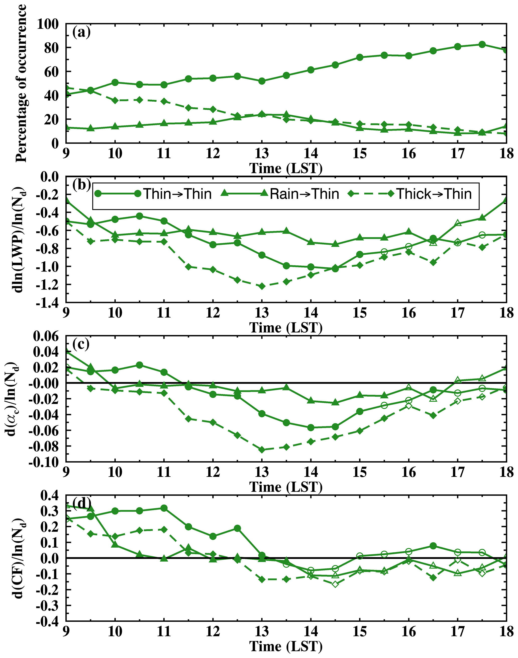
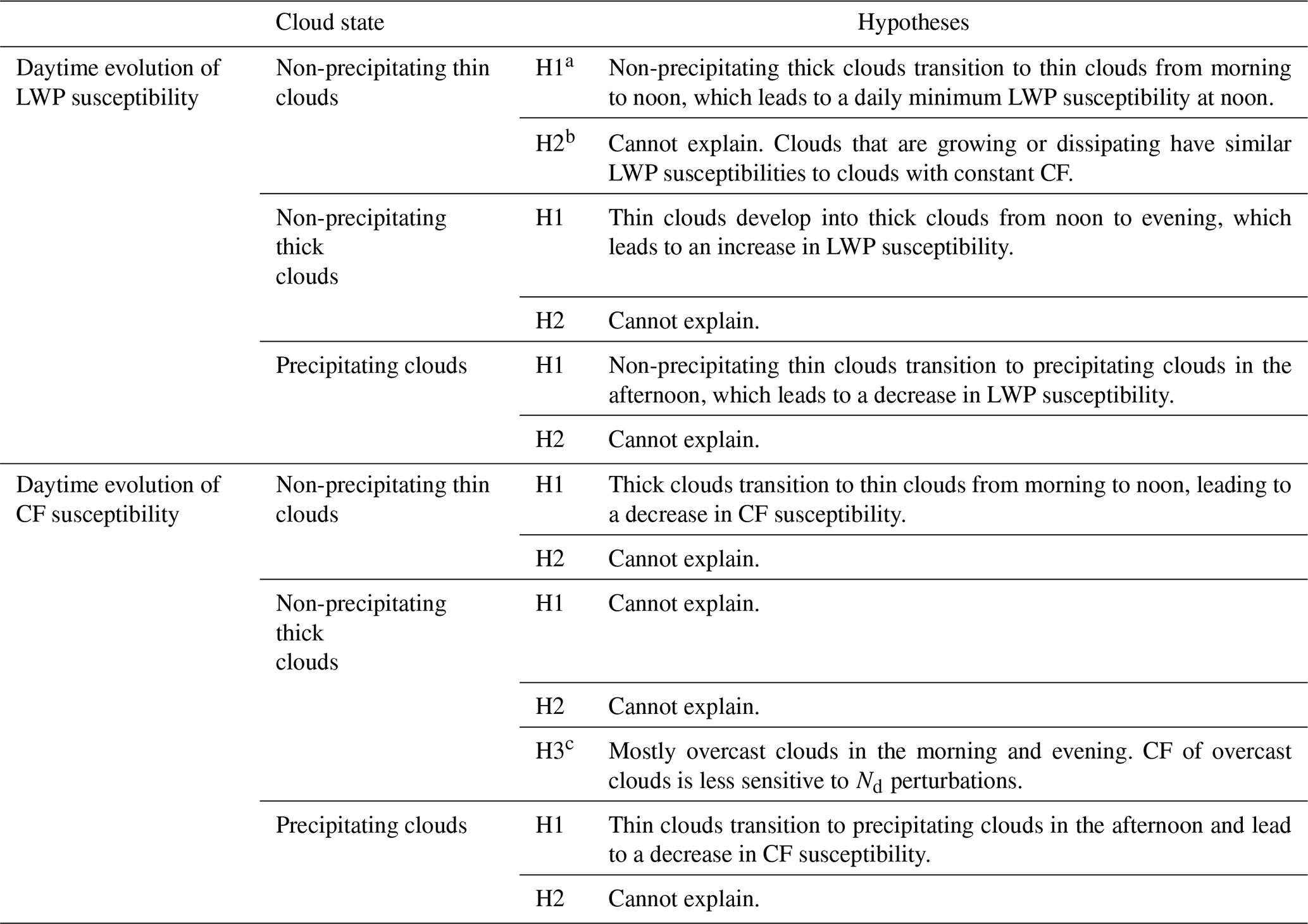
Figure 5 Daytime variation in non-precipitating thin clouds transitioning from non-precipitating thin clouds (thin → thin, solid line with circle symbols), precipitating clouds (rain → thin, solid line with triangle symbols), and non-precipitating thick clouds (thick → thin, dashed line with diamond symbols) in the previous 2 h. Symbols for different state transitions are noted in (b). In (b)–(d), filled markers indicate data points that are significantly different from the two other groups (p < 0.05), while open markers indicate statistical insignificance.

Hypothesis H1 is related to the response time of cloud LWP and CF to N_d perturbations. Both numerical models and observations have shown that the influence of aerosols on cloud LWP, achieved through adjusting the entrainment rate, may take 4 h to become apparent and up to 20 h to reach an equilibrium (e.g., Glassmeier et al., 2021; Gryspeerdt et al., 2021; Fons et al., 2023). Similarly, CF increases gradually from increasing aerosols and may take approximately 3 to 4 h to reach its maximum effect after the initial perturbation (Gryspeerdt et al., 2021). Therefore, we hypothesize that if clouds change state during the adjustment time, clouds may still retain the “memory” of their responses to N_d perturbations from the previous state. The possible physical processes and mechanisms for this hypothesis include the LWP susceptibility being mainly driven by cloud-top evaporation and the entrainment rate. The positive feedbacks among entrainment, evaporative cooling, longwave radiative cooling, and mixing from the cloud top form a positive feedback loop and set up an environment conducive to enhanced entrainment and evaporation. These feedbacks and the environment will not change immediately even when the cloud LWP decreases and clouds transition to a thin state or vice versa. The diurnal variation in cloud properties and transition in cloud state lead to a diurnal evolution in cloud susceptibility.

To quantify the dependence of current cloud susceptibility on previous cloud states, we track the cloud state for each 1° × 1° box backward in time for 2 h and classify the non-precipitating thin clouds into three groups (Fig. 5): (1) thin clouds that are currently classified as thin clouds and did not change states in the past 2 h (thin → thin), (2) thin clouds that evolved from precipitating clouds (rain → thin), and (3) thin clouds that decayed from non-precipitating thick clouds (thick → thin). This backward-tracking classification is applied at each time step. As shown in Fig. 5a, at 09:00 LST, ∼ 50 % of the non-precipitating thin clouds originate from thick clouds in previous hours. The transition from thick to thin clouds is likely caused by the increased solar radiation after sunrise, leading to clouds decoupling from the ocean surface and a decrease in cloud LWP. In the evening, on the other hand, around 80 % of the thin clouds are thin clouds in previous hours. In addition, fewer than 20 % of the non-precipitating thin clouds transition from precipitating clouds.

Consistently with our hypothesis, non-precipitating thin clouds that were previously thick have significantly more negative LWP and α_c susceptibilities than thin clouds that were previously thin or precipitating (Fig. 5b and c). The differences between the two categories are most pronounced from late morning to early afternoon and less pronounced in the early morning and evening. Such a pattern is likely attributable to the daytime evolution of the marine boundary layer and cloud coupling state. For example, in the early morning (e.g., 09:00–10:00 LST), even with a higher frequency of occurrence of thick clouds transitioning to thin clouds, the LWP susceptibility for the thick-to-thin category is less negative compared to later times (dashed line with diamond symbols in Fig. 5a and b). This is attributed to the less negative LWP susceptibility for non-precipitating thick clouds at earlier times (e.g., 07:00–09:00 LST, not shown), in connection with a well-mixed boundary layer that is able to transport moisture from the ocean to the cloud, which compensates for the moisture loss from aerosol-enhanced entrainment (e.g., Sandu et al., 2008) so that both thick and thin clouds exhibit less negative LWP susceptibilities. From late morning to early afternoon, with increasing solar radiation, deepening of the boundary layer, and clouds decoupled from the surface, LWP susceptibility for thick clouds largely decreases and reaches a daily minimum, which contributes to the largest difference between the thin-to-thin and thick-to-thin categories shown in Fig. 5b. The opposite processes occur from afternoon to evening: LWPs of thick clouds become less susceptible to N_d perturbations, and the difference between the two categories is less pronounced. These results support our hypothesis that clouds retain the memory of their responses to N_d perturbations from their previous states.

Similarly to LWP, responses of CF to N_d perturbations in the morning retain the memory of the previous states of clouds. As seen in Fig. 5d, thin clouds that transitioned from thick clouds or precipitating clouds have significantly less positive CF susceptibility than thin clouds that were previously thin, particularly in the morning. As the CF susceptibility for thin clouds that evolved from precipitating and thick clouds greatly decreases from morning to noon, the CF susceptibility for thin clouds decreases from large positive to near zero from morning to noon (Fig. 4c). A maximum in CF susceptibility in the early morning is likely associated with the influence of aerosols on boundary layer mixing and the evolution of the boundary layer from morning to noon. The enhanced entrainment rate and radiative cooling rate from N_d perturbations help to destabilize the boundary layer and transport moisture from the ocean surface to clouds, facilitating new cloud formation (e.g., Christensen et al., 2020). As the boundary layer is typically well mixed in the morning with clouds coupled to the surface, the impact of aerosols on CF is strongest in the morning and gradually decreases from morning to noon. In the afternoon, thin clouds transitioning from all three states have near-zero CF responses to N_d perturbations. Further analyses and model simulations are needed to better understand the impacts of aerosols and the associated diurnal evolution of the entrainment rate and boundary layer mixing on cloud cover and lifetime, to better explain the observed daytime variation in CF susceptibility for non-precipitating thin clouds.

Lastly, the impact of the cloud memory of the AIE on current cloud susceptibility is also evident within a 30 min window when a transition of the cloud state has just occurred (Fig. S4 in the Supplement). Consistent with the findings in Fig. 5, thin clouds that transition from thick clouds exhibit much more negative LWP and α_c susceptibilities compared to thin clouds that remain thin during the 30 min. Yet, the number of cases experiencing a transition in cloud state within a 30 min window is limited (Fig. S4a). In addition, the impact of the transition in cloud state on the current cloud susceptibility persists for at least 4 h (Fig. S5 in the Supplement). As our tracking method does not follow individual cloud parcels to track changes in their states, the influence of cloud advection may become significant over longer tracking times, such as 4 h. Therefore, a 2 h tracking window is used in this study.

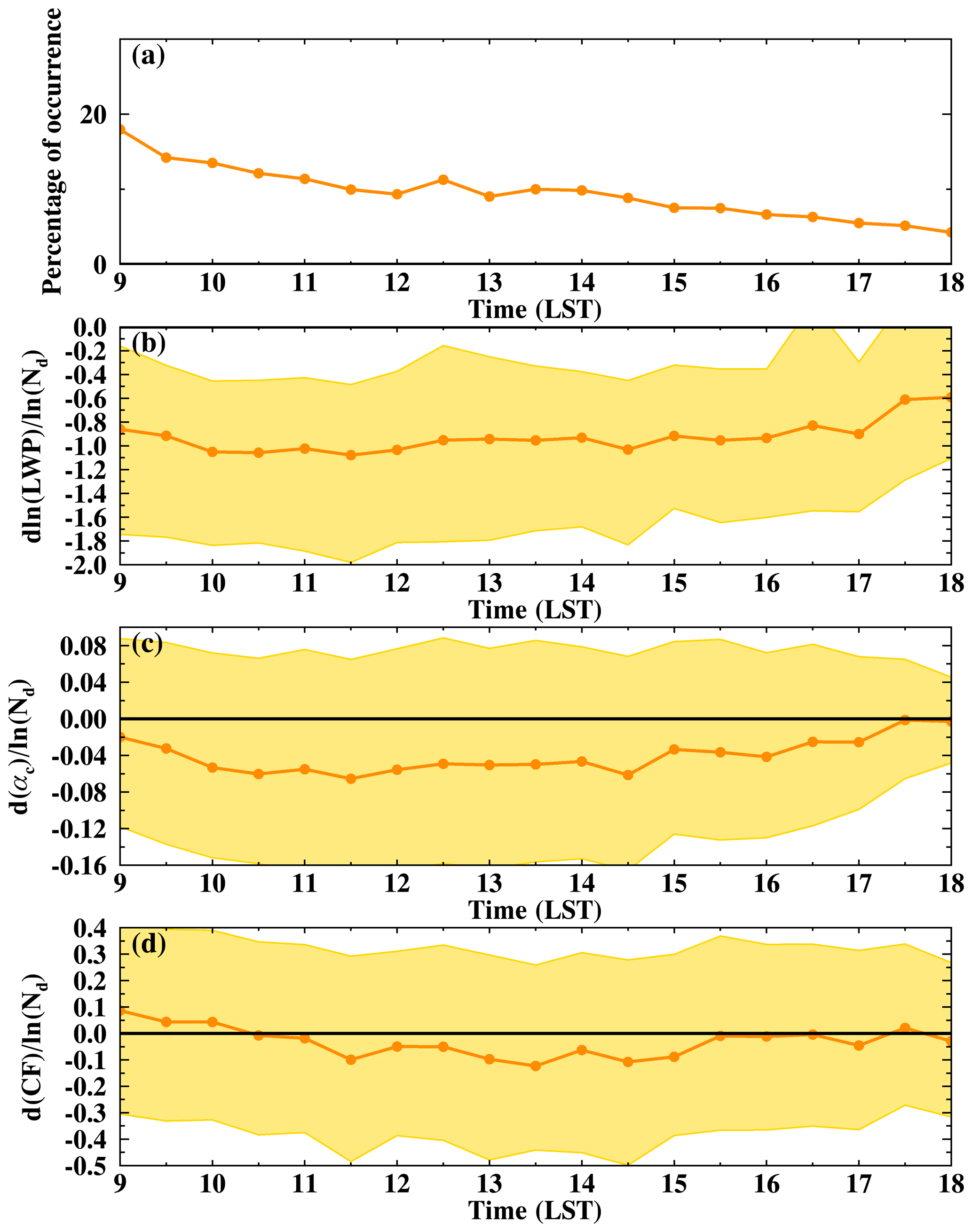
Figure 6 Daytime variation in (a) the occurrence of non-precipitating thick clouds as a percentage of warm boundary layer clouds, (b) cloud LWP susceptibility ($\mathrm{d}\text{ln}\left(\mathrm{LWP}\right)/\mathrm{d}\text{ln}\left(N_{\mathrm{d}}\right))$, (c) cloud albedo susceptibility ($\mathrm{d}{\mathit{\alpha }}_{\mathrm{c}}/\mathrm{d}\text{ln}\left(N_{\mathrm{d}}\right))$, and (d) cloud fraction susceptibility ($\mathrm{d}\mathrm{CF}/\mathrm{d}\text{ln}\left(N_{\mathrm{d}}\right))$ for non-precipitating thick clouds. The shaded areas represent the lower and upper 25th percentiles of the cloud susceptibilities for each time step, and the solid lines with dots represent the mean values.

As discussed in the “Dataset and methodology” section, while the advective effects in our study are expected to be modest, we further isolate their impact by performing an analysis for cloud scenes with wind speeds of less than 7 m s⁻¹ (60 % of time) when clouds are somewhat stationary in the 2 h period. The influence of transition in cloud state is consistent with Fig. 5, with more negative LWP and α_c susceptibilities for thin clouds transitioning from thick clouds, while the signal is slightly stronger (not shown). This consistency confirms that our tracking method can capture the signal of the cloud state transition and its impact on cloud susceptibilities during summer in the study region.

In summary, the U-shaped daytime variations in LWP and α_c susceptibilities for non-precipitating thin clouds are likely due to clouds retaining the memory of the AIE. From morning to noon, as non-precipitating thick clouds evolve into thin clouds, they retain their memory of the large negative LWP susceptibility. Therefore, both LWP and α_c susceptibilities decrease from morning to noon for thin clouds and reach their daily minima at noon. In the afternoon, as a growing percentage of thin clouds persist as thin clouds during the following hours, LWP and α_c susceptibilities gradually increase to less negative and near zero, respectively.

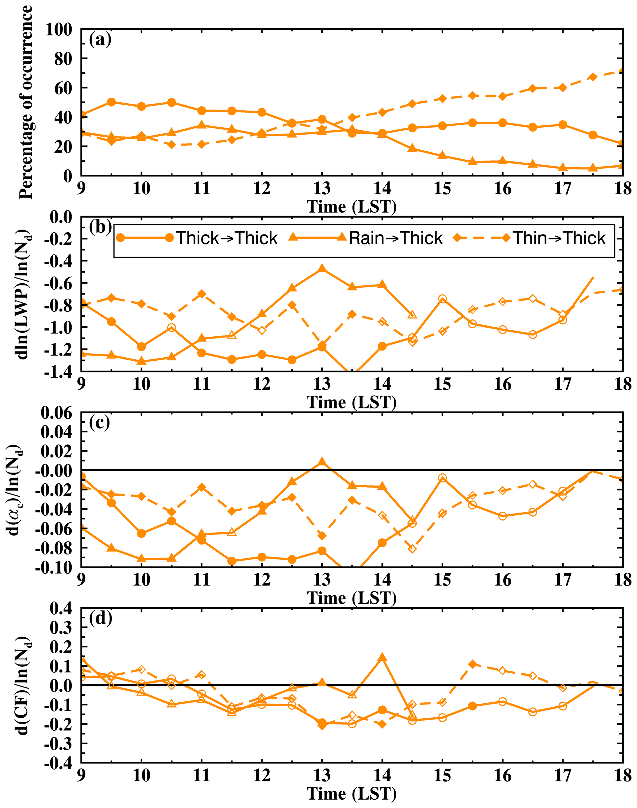
Figure 7 Daytime variation in non-precipitating thick clouds transitioning from non-precipitating thick clouds (thick → thick, solid line with circle symbols), precipitating clouds (rain → thick, solid line with triangle symbols), and non-precipitating thin clouds (thin → thick, dashed line with diamond symbols) in the previous 2 h. Symbols for different state transitions are noted in (b). In (b)–(d), filled markers indicate data points that are significantly different from the two other groups (p < 0.05), while open markers indicate statistical insignificance.

3.4.2 Non-precipitating thick clouds

Consistent with Fig. 2e, non-precipitating thick clouds are the least frequent warm boundary layer cloud state during summer over the ENA region. Their percentage of occurrence continuously decreases from 20 % in the morning to less than 5 % in the evening (Fig. 6a). For LWP and α_c, their susceptibilities first decrease from less negative to more negative in the morning and then increase from noon to evening (Fig. 6b and c, respectively). CF susceptibility is weakly positive in the early morning, becomes weakly negative from late morning to early afternoon, and increases to near zero in the evening (Fig. 6d). The daytime evolutions of LWP and α_c susceptibilities for thick clouds exhibit a consistent trend with cloud susceptibilities for thin clouds transitioning from thick clouds shown in Fig. 5 but with a lag of 2 h. For example, the LWP susceptibility for thick clouds decreases from −0.8 to −1.1 from 09:00 to 11:00 LST and it increases from −1.1 to −0.8 from 11:00 to 16:00 LST (Fig. 6b), while the LWP susceptibility for the thick-to-thin category in Fig. 5b decreases from −0.8 to −1.2 from 11:00–13:00 LST and increases to −0.6 from 13:00 to 18:00 LST. This result supports our hypothesis on clouds retaining their memory of the AIE of their previous cloud state.

To gain insight into the observed evolution of LWP and α_c susceptibility from morning to evening, we investigate the influence of the cloud state transition on cloud susceptibility for non-precipitating thick clouds, which is summarized as H1 in Table 1. As shown in Fig. 7a, around 40 % of thick clouds are sustained as thick clouds from the previous 2 h in the morning, whereas during the late afternoon to evening, with decreasing solar radiation, more than 60 % of thick clouds are developed from thin clouds. Consistently with the findings presented in Fig. 5, thick clouds that were previously thick exhibit significantly more negative LWP susceptibility compared to thick clouds that were previously thin (Fig. 7b). These differences are particularly prominent from late morning to noon and become insignificant in the afternoon. As discussed before, the difference between the thick-to-thick and the thin-to-thick categories is due to the LWP susceptibilities for thick and thin clouds of previous times, while the smaller differences in the early morning and afternoon could be attributed to the expected stronger turbulence and cloud coupling at these times. Additionally, Fig. 7d indicates that transition in cloud state cannot explain the daytime variation in CF susceptibility for thick clouds, as all three groups are insignificantly different from each other.

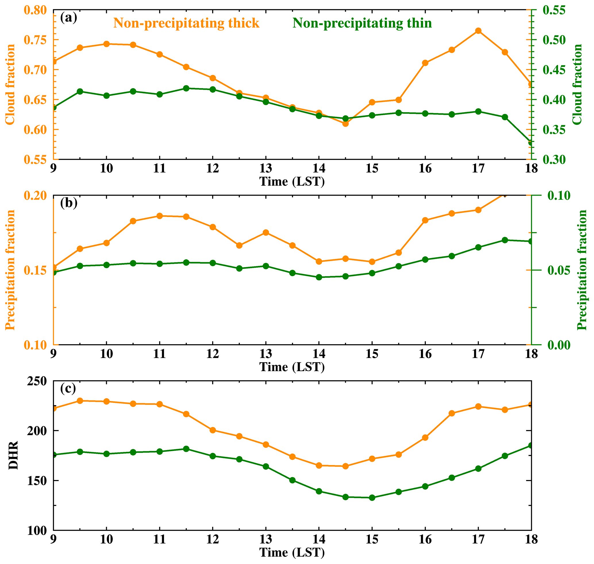
Figure 8 Diurnal variation in the (a) cloud fraction, (b) pixel-level precipitation fraction, and (c) diameter-to-height ratio (DHR) for non-precipitating clouds. Different colors represent different cloud states as indicated in (a). Please note that the non-precipitating thin cloud in (a) and (b) uses the y axis on the right side.

To understand the driving mechanism for the daytime variation in CF susceptibility shown in Fig. 6d, we calculate the mean cloud properties for non-precipitating thin and thick clouds, as shown in Fig. 8. In the morning, non-precipitating thick clouds are predominantly overcast clouds with a mean CF of 75 % (Fig. 8a). To distinguish between overcast and broken clouds, we calculate the diameter-to-height ratio (DHR) for each cloud, where the diameter is estimated by the square root of the area and height is defined as the 90th percentile of cloud tops. As shown in Fig. 8c, thick clouds are mostly overcast in the morning with a mean DHR of 230. Compared to broken clouds, overcast clouds have less room for CF to increase, which results in a less positive CF susceptibility for thick clouds compared to thin. After 10:00 LST, non-precipitating thick clouds start to break. The mean CF decreases from 75 % at 10:00 LST to 60 % at 14:00 LST, and the DHR decreases from 230 to 170. As CF for broken clouds is more sensitive to N_d perturbations, CF susceptibility decreases to −0.13 ln(N_d)⁻¹, which is consistent with the daytime mean negative CF susceptibility shown in Fig. 2c. From afternoon to evening, clouds transition to overcast again (Fig. 8), and the CF susceptibility increases back to zero. This impact of cloud morphology (e.g., overcast or broken clouds) on daytime variation in CF susceptibility is summarized as H3 in Table 1.

The previous results are summarized as follows: LWP susceptibility for non-precipitating thick clouds first decreases from less negative to more negative in the morning and then increases from noon to evening, which is likely attributable to the transition from thin to thick clouds. In the morning, 40 % to 50 % of thick clouds were previously thick clouds; these clouds exhibit a large negative LWP susceptibility. In the afternoon, an increasing percentage of thick clouds develop from thin clouds and retain the memory of LWP responses to N_d perturbations of the thin clouds. LWP susceptibility gradually increases and becomes similar to that of thin clouds (Figs. 4b and 6b). Daytime variation in CF susceptibility for thick clouds is likely attributable to changes in cloud morphology. In the morning and evening, thick clouds are mostly overcast with CF less sensitive to N_d perturbations, resulting in a near-zero CF susceptibility. From late morning to early afternoon, the overcast thick clouds break down and CF decreases with increasing N_d, likely due to the increased shortwave absorption, the enhanced entrainment, and evaporation.

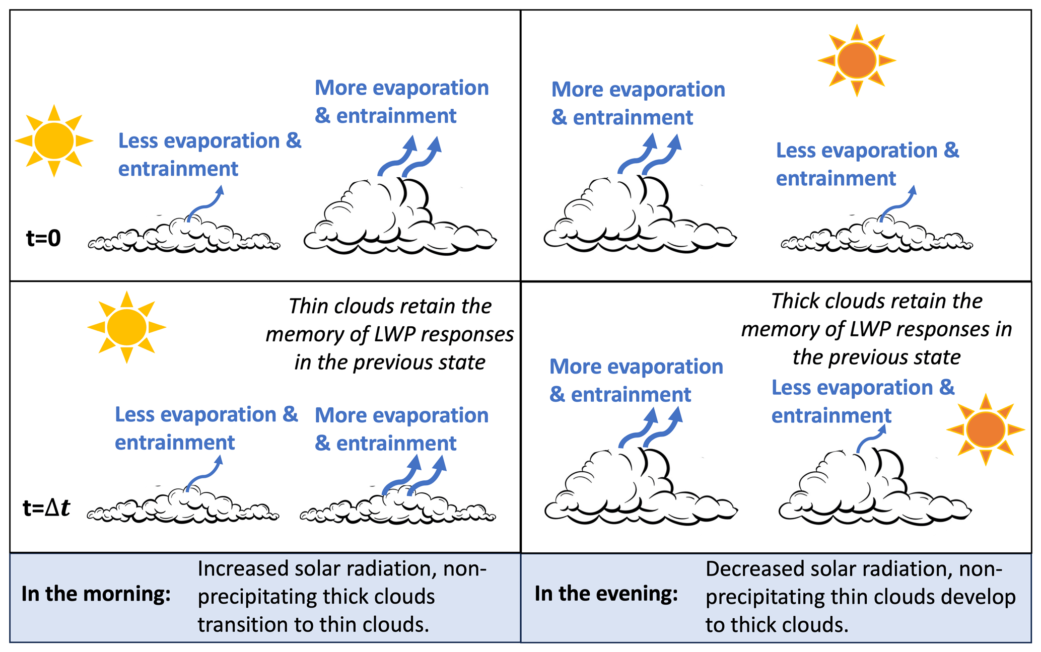
Figure 9 Schematic figure of the influence of cloud memory and transition of cloud state on the LWP susceptibility and its daytime variation.

The impact of cloud memory and the transition of cloud state on the daytime variation in LWP susceptibility is summarized as a schematic figure shown in Fig. 9. From morning to noon, as non-precipitating thick clouds transition to thin clouds, thin clouds retain their memory of the AIE of their previous state. Therefore, LWP susceptibility for thin clouds decreases from morning to noon and reaches its daily minimum in the early afternoon. From early afternoon to evening, with non-precipitating thin clouds developing into thick clouds, LWP susceptibility for thick clouds increases.

3.4.3 Precipitating clouds

Precipitating clouds, depicted in Fig. 10a, are the dominant cloud state in this region, accounting for 46 % of the warm boundary layer clouds, compared to 44 % of non-precipitating thin clouds. The frequency of precipitating clouds is higher in the morning and evening compared to noon. Throughout the day, the mean LWP susceptibility remains consistently negative, fluctuating between −0.5 and −0.3, with minimum values between 14:00–16:00 LST (Fig. 10b). The daytime variability in LWP susceptibility for precipitating clouds is much lower than that for non-precipitating thin (e.g., from −0.9 to −0.4) and thick (e.g., from −1.1 to −0.6) clouds. The negative LWP susceptibility is likely due to the prevalence of lightly precipitating clouds, with a mean precipitating fraction ranging from 0.2 to 0.5 (Fig. S2d). The influence of precipitation suppression is smaller than that of the entrainment enhancement. Similarly, α_c susceptibility fluctuates between 0 and 0.02 throughout the day, with near-zero α_c susceptibility in the early afternoon (Fig. 10c). Despite the minimal daytime variation, the LWP and α_c susceptibilities at 13:00–16:00 LST are statistically significantly different from cloud susceptibilities in the morning and evening at a 95 % confidence level with a two-tailed t test. The CF susceptibility for precipitating clouds also shows minimal daytime variation compared to non-precipitating clouds, with a mean value ranging from 0 to 0.1 (Fig. 10d).

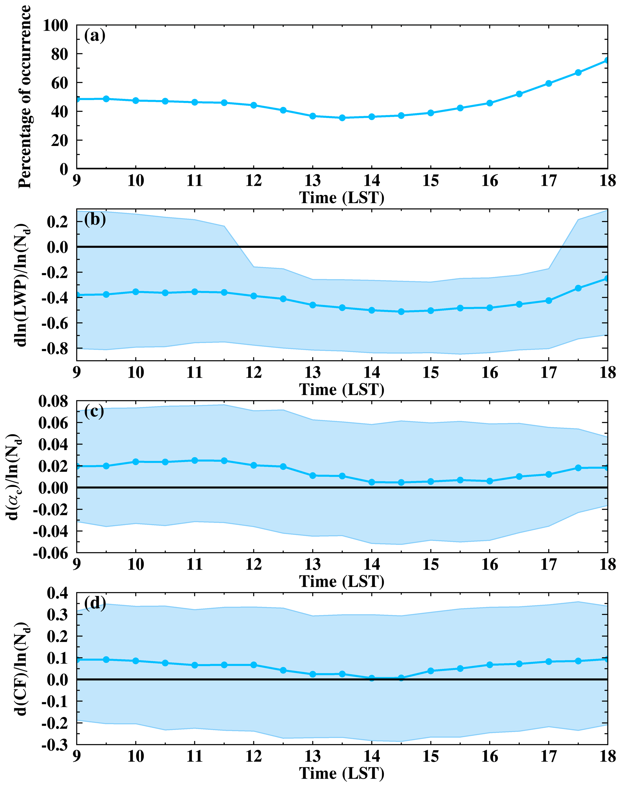
Figure 10 Daytime variation in (a) the occurrence of precipitating clouds as a percentage of warm boundary layer clouds, (b) cloud LWP susceptibility ($\mathrm{d}\text{ln}\left(\mathrm{LWP}\right)/\mathrm{d}\text{ln}\left(N_{\mathrm{d}}\right))$, (c) cloud albedo susceptibility ($\mathrm{d}{\mathit{\alpha }}_{\mathrm{c}}/\mathrm{d}\text{ln}\left(N_{\mathrm{d}}\right))$, and (d) cloud fraction susceptibility ($\mathrm{d}\mathrm{CF}/\mathrm{d}\text{ln}\left(N_{\mathrm{d}}\right))$ for precipitating clouds. The shaded areas represent the lower and upper 25th percentiles of the cloud susceptibilities for each time step.

Consistent with non-precipitating clouds, the daytime variation in LWP and α_c susceptibilities for precipitating clouds can be attributed to the transition of cloud states. For example, as shown in Fig. 11b–d, precipitating clouds that transition from non-precipitating thin clouds exhibit significantly more negative/less positive cloud susceptibilities than precipitating clouds that were previously precipitating. Meanwhile, α_c and CF susceptibilities switch signs from positive to negative in the afternoon for precipitating clouds that transition from non-precipitating thin clouds compared to those that were previously precipitating (dashed line with diamond symbols in Fig. 11c and d). Starting from 13:00 LST, when non-precipitating thin clouds transition to precipitating clouds (Fig. 11a), LWP and α_c susceptibilities begin to decrease and reach their daily minimum in the late afternoon. Interestingly, as non-precipitating clouds transition to precipitating clouds (Fig. 11b and c, thin → rain, thick → rain), their LWP and α_c susceptibilities exhibit both less negative values and smaller daytime variations compared to thin/thick clouds that remain thin/thick (Fig. 5b and c, thin → thin; Fig. 7b and c, thick → thick). The underlying reason for this observation is currently unclear and warrants further investigation into the sensitivity of the AIE for clouds experiencing transition in cloud states, especially between precipitating and non-precipitating clouds. Lastly, the percentage of precipitating clouds that transition from non-precipitating thick clouds is less than 7 % (Fig. 11a).

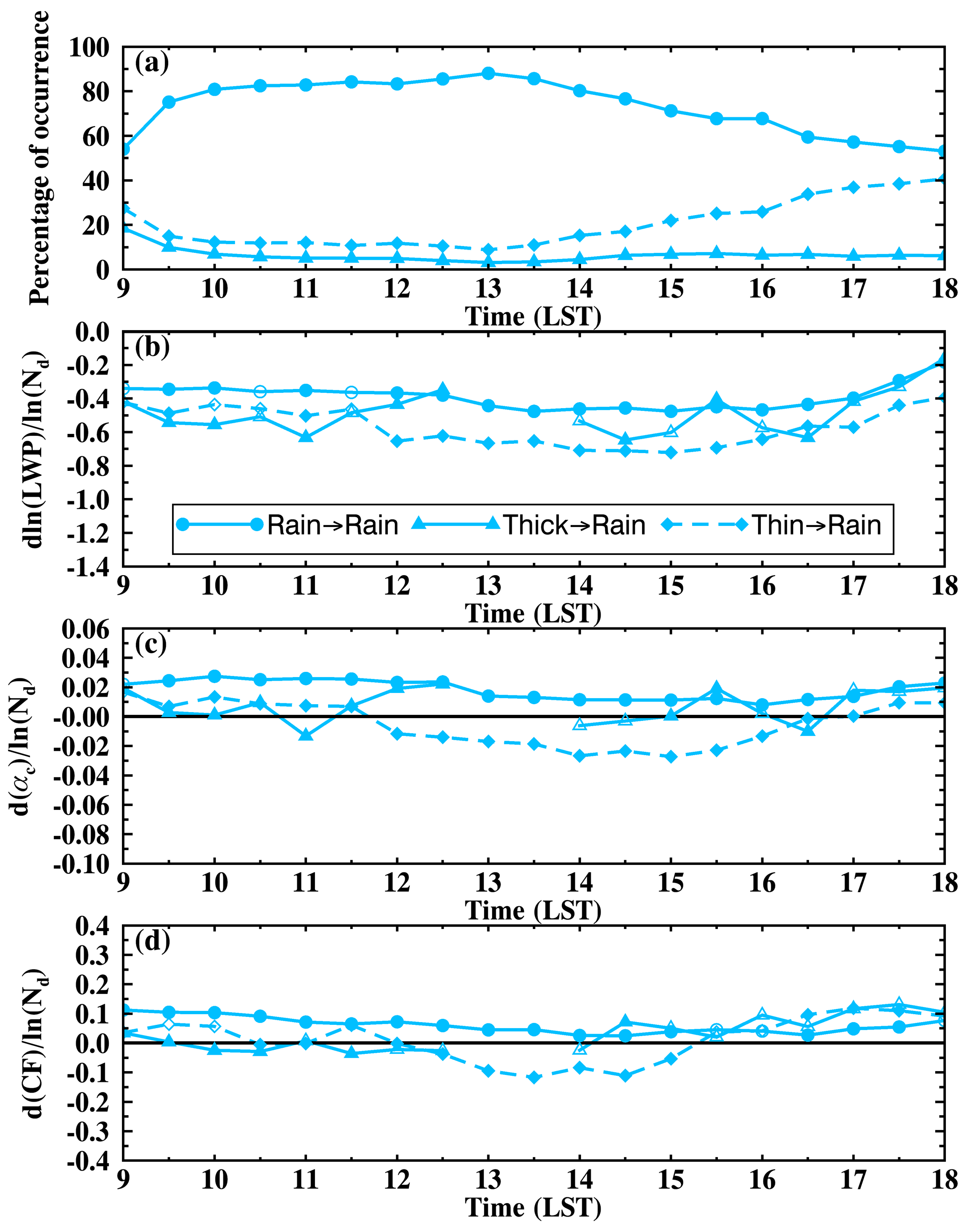
Figure 11 Daytime variation in precipitating clouds transitioning from precipitating clouds (rain → rain, solid line with circle symbols), non-precipitating thick clouds (thick → rain, solid line with triangle symbols), and non-precipitating thin clouds (thin → rain, dashed line with diamond symbols) in the previous 2 h. Symbols for different state transitions are noted in (b). In (b)–(d), filled markers indicate data points that are significantly different from the two other groups (p < 0.05), while open markers indicate statistical insignificance.

In conclusion, precipitating clouds exhibit smaller daytime variation in cloud susceptibilities compared to non-precipitating thin and thick clouds. The decrease in LWP and α_c susceptibilities for precipitating clouds in the afternoon is likely contributed to by the transition of non-precipitating thin clouds to precipitating clouds.

Combining the results shown here and results in Sect. 3.4.1, we can answer the question of which cloud state contributes the most to the daytime variation in cloud susceptibility. The non-precipitating thin clouds exhibit similar daytime variations in LWP, α_c, and CF susceptibility to the warm boundary layer clouds (Fig. 4 vs. Fig. 3), with clouds being less susceptible to N_d perturbations in the morning and evening and more susceptible at noon. Additionally, non-precipitating thin clouds have the highest frequency at noon. On the other hand, precipitating clouds, despite their higher percentage of occurrence than thin clouds, exhibit minimal daytime variation in cloud susceptibility. Therefore, the pronounced daytime variations in cloud susceptibilities for warm boundary layer clouds primarily stem from non-precipitating thin clouds. The distinct daytime evolution patterns for the three cloud states highlight the importance of cloud state classification in quantification of cloud susceptibility.

3.5 Contribution to the daytime variation in cloud susceptibility

As discussed in the previous section, both the frequency of occurrence of cloud states and the intensity of cloud responses to N_d perturbations exhibit pronounced daytime variations. In this section, we aim to compare the contribution of these two components to the overall daytime variation in cloud susceptibilities by fixing one component constant at a time. The contribution from changes in the frequency of cloud states is represented by the red lines in Fig. 12, which are estimated by weighting the daytime mean cloud susceptibility (Fig. 2a–c) with the half-hourly frequency of occurrence of clouds in the LWP–N_d parameter space, assuming a constant intensity of cloud susceptibility during the daytime. The contribution from changes in the intensity of cloud susceptibility is depicted by the blue lines, which are estimated by weighting the half-hourly cloud susceptibility in the LWP–N_d parameter space with the daytime mean frequency of occurrence of clouds (Fig. 2e), assuming a constant frequency during the daytime. The black line in Fig. 12 represents the observed susceptibility shown in Fig. 3, and it includes the contributions from daytime variations in both components.

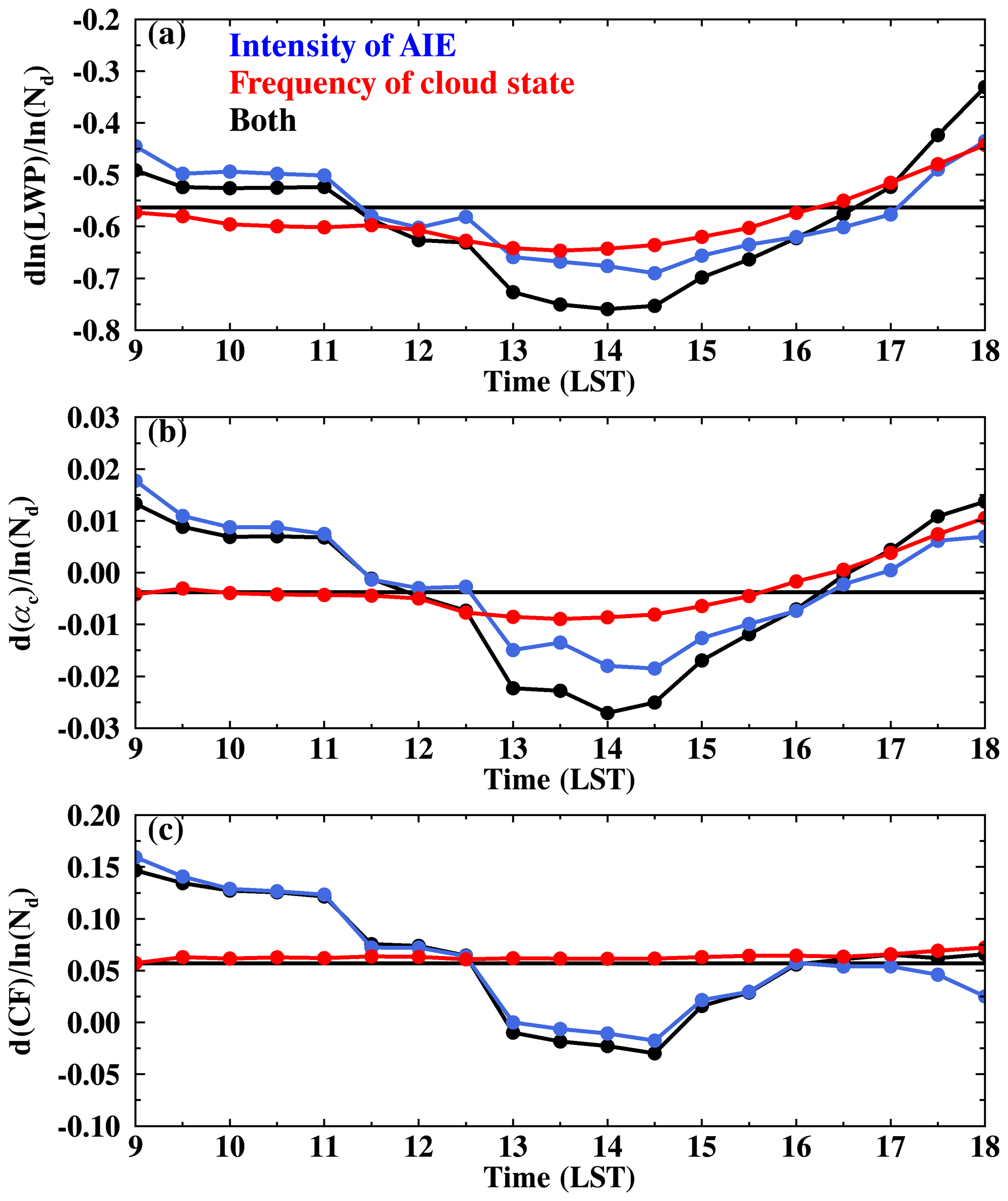
Figure 12 Daytime variation in cloud susceptibility contributed from the variability in the intensity of susceptibility (blue lines with symbols), variability in the frequency of occurrence of cloud state (red lines with symbols), and both (black lines with symbols). (a) Cloud LWP susceptibility ($\mathrm{d}\text{ln}\left(\mathrm{LWP}\right)/\mathrm{d}\text{ln}\left(N_{\mathrm{d}}\right))$; (b) cloud albedo susceptibility ($\mathrm{d}{\mathit{\alpha }}_{\mathrm{c}}/\mathrm{d}\text{ln}\left(N_{\mathrm{d}}\right))$; (c) cloud fraction susceptibility ($\mathrm{d}\mathrm{CF}/\mathrm{d}\text{ln}\left(N_{\mathrm{d}}\right))$. The horizontal solid black lines in (a)–(c) are the daytime mean susceptibility.

When comparing the net observed daytime variation in cloud susceptibilities (black lines) with the contributions from changes in the intensity and the frequency of cloud state (blue and red lines, respectively), we find that the daytime changes in cloud susceptibility are primarily driven by changes in the intensity of cloud susceptibilities during the day. Additionally, as shown in Fig. 12a and b, the red lines are close to the daytime mean values in the morning, which indicates that variations in the frequency of different cloud states have a minimal impact on changes in LWP and α_c susceptibilities in the morning. On the other hand, in the afternoon, both shifts in cloud states and changes in intensities contribute to the changes in LWP and α_c susceptibilities. Compared with LWP and α_c susceptibilities, the daytime variation in CF susceptibility shows minimal sensitivity to changes in the cloud state frequency. This limited impact stems from the fact that the daytime fluctuation in the cloud state frequency is predominantly influenced by precipitating and non-precipitating thin clouds. Meanwhile, the daytime mean CF susceptibilities for precipitating and non-precipitating thin clouds closely align, measuring 0.08 and 0.09, respectively (Fig. 2c). This convergence diminishes the influence of alterations in the frequency of these two cloud states.

In summary, the daytime variation in cloud susceptibility is largely driven by the variation in its intensity. Since polar-orbiting satellites only observe the cloud responses to N_d perturbations across different cloud states at their overpass time, they cannot fully capture the diurnal variation in cloud susceptibilities driven by the variation in the intensity of cloud susceptibility. Given that all three cloud susceptibilities reach their daily minimum at around 13:30 LST, studies based on polar-orbiting satellites with overpass times at noon may underestimate the daily mean value of cloud susceptibility.

4 Discussions

In this study, we quantify the susceptibility of warm boundary layer clouds to N_d perturbation using the pixel-level SEVIRI cloud retrievals of each time step. For heavily precipitating clouds, LWP increases under pristine conditions (e.g., N_d < 30 cm⁻³, Fig. 2a). For lightly precipitating and non-precipitating clouds, LWP decreases with N_d. The N_d–LWP relationship found in this study is consistent with that in Gryspeerdt et al. (2019) using global mean cloud retrievals from MODIS and AMSR-E at a coarser resolution of 1° × 1° and daily timescale. This consistency between different satellite measurements at different temporal and spatial scales greatly enhances our confidence in the retrieved relationship.

This study further separates non-precipitating clouds into thin and thick clouds based on their LWP. A consistent decreasing trend in cloud water is found for both states, yet non-precipitating thick clouds exhibit more negative LWP susceptibility $\left(\frac{\mathrm{d}\text{ln}\left(\mathrm{LWP}\right)}{\mathrm{d}\text{ln}\left(N_{\mathrm{d}}\right)}=-\mathrm{0.94}\right)$ compared to thin clouds $\left(\frac{\mathrm{d}\text{ln}\left(\mathrm{LWP}\right)}{\mathrm{d}\text{ln}\left(N_{\mathrm{d}}\right)}=-\mathrm{0.71}\right)$. The LWP susceptibilities estimated in this study are more negative than those in Zhang et al. (2022) and Zhang and Feingold (2023), based on a similar classification of cloud states. Particularly, we found that non-precipitating thin clouds have a decreasing trend in cloud water and a warming effect at the surface radiation while these are opposite in Zhang et al. (2022) and Zhang and Feingold (2023). This is due to different seasons and study regions between our study and their studies. The summer boundary layer in the ENA region is deeper and less stable with higher cloud tops (e.g., Klein and Hartmann, 1993; Ding et al., 2021; King et al., 2013) compared to the NE Pacific in Zhang et al. (2022) and the NE Atlantic region in Zhang and Feingold (2023). The less stable condition, deeper boundary layer, and deeper clouds could lead to a stronger cloud-top entrainment rate and result in a more negative LWP susceptibility (Possner et al., 2020; Toll et al., 2019).

Regarding the CF adjustment to N_d perturbation, a daytime mean positive response is found for precipitating and non-precipitating thin clouds and a negative response for non-precipitating thick clouds (Fig. 2c). Few studies have quantified the CF adjustment rate at 30 min intervals for a direct comparison of CF susceptibility. However, similar results are found using measurements and retrievals from different platforms at various spatial scales and timescales, which greatly increases our confidence in the observed CF responses toward N_d perturbation. For example, using MODIS measurement, Kaufman et al. (2005) found an increase in the longitudinal mean cloudiness for warm boundary layer clouds with increasing AOD in all four regions of the Atlantic Ocean characterized by distinct aerosol types. Using the natural experiment of volcanic eruption at Holuhraun in Iceland, Chen et al. (2022) found that aerosols from the eruption increase the monthly mean cloud cover by 10 % over the North Atlantic. By tracking the cloud trajectory using geostationary satellites, Christensen et al. (2020) found that aerosols enhance both CF and cloud lifetime at the timescale of 2–3 d, especially under stable conditions. It is worth noting that a decrease in CF was not observed in these studies, likely due to the prevalence of non-precipitating thin clouds and precipitating clouds in the Atlantic or the NE Pacific (e.g., Zhang and Feingold, 2023) that mask the signal from non-precipitating thick clouds without distinguishing cloud states.

Lastly, the distinct U-shaped daytime variation in all three cloud properties found in this study (Fig. 3a–c) is unlikely to be due to the systematic bias in r_e and τ retrievals at large SZAs based on the following two aspects. Firstly, if the daytime variation were driven by retrieval bias at large SZAs, we would expect the susceptibility to exhibit a symmetric pattern at local noon. As shown in Figs. 10 and 6, the LWP and α_c susceptibilities for precipitating and non-precipitating thick clouds exhibit asymmetric patterns at local noon: with a decreasing trend from 13:00 LST and daily minimum at 16:00 LST and a continuously increasing trend from 11:00 to 18:00 LST, respectively. In addition, the CF susceptibilities for all three cloud states show asymmetric patterns at local noon. Secondly, if the retrieval uncertainty were to dominate the signal, we would expect less variation in cloud susceptibilities for overcast clouds, which suffer lower uncertainties in cloud retrievals from the plane-parallel assumption and the cloud 3-D effect. However, the opposite is found from the sensitivity test where overcast clouds exhibit stronger daytime variation in cloud susceptibilities (not shown).

5 Conclusions

Using N_d as an intermediary variable, this study investigates the aerosol indirect effect (AIE) for warm boundary layer clouds and its daytime variation over the ENA region with the half-hourly and 3 km cloud property retrievals from SEVIRI on Meteosat-11. To constrain meteorological impacts on clouds and aerosol–cloud interaction, cloud susceptibilities are estimated within a 1° × 1° grid box for each satellite time step. Based on the daytime mean cloud susceptibilities in the LWP–N_d parameter space, the sign and magnitude of cloud susceptibilities strongly depend on the cloud states (Fig. 2). Accordingly, warm boundary layer clouds are classified into three states: precipitating clouds (r_e > 15 µm), non-precipitating thick clouds (r_e < 15 µm, LWP > 75 g m⁻²), and non-precipitating thin clouds (r_e < 15 µm, LWP < 75 g m⁻²).

Precipitating clouds exhibit contrasting responses in cloud LWP, with increases observed for heavily precipitating clouds and decreases for lightly precipitating clouds. Positive α_c and CF susceptibilities are identified for both heavily and lightly precipitating clouds. The net all-sky radiative forcing of the AIE on precipitating clouds is estimated to be −13 $\mathrm{W}{\mathrm{m}}^{-\mathrm{2}}\ln (N_{\mathrm{d}}{)}^{-\mathrm{1}}$, with contributions from the CF and α_c effects of −9.5 and −3.5 $\mathrm{W}{\mathrm{m}}^{-\mathrm{2}}\ln (N_{\mathrm{d}}{)}^{-\mathrm{1}}$, respectively. For non-precipitating clouds, both thick and thin clouds show negative LWP susceptibility with more negative values found for thick clouds with higher LWP and N_d. This is likely attributable to the stronger shortwave absorption, larger cloud-top radiative cooling rate, and stronger entrainment for thick clouds. Consistent with the evaporation–entrainment feedback, non-precipitating thick clouds exhibit a decrease in CF and α_c with increasing N_d and result in a net warming effect at the surface and a radiative forcing of +4.4 $\mathrm{W}{\mathrm{m}}^{-\mathrm{2}}\ln (N_{\mathrm{d}}{)}^{-\mathrm{1}}$. On the other hand, non-precipitating thin clouds show an increasing response in CF and a less negative α_c susceptibility. Additionally, the radiative effect from increasing CF (−8.3 $\mathrm{W}{\mathrm{m}}^{-\mathrm{2}}\ln (N_{\mathrm{d}}{)}^{-\mathrm{1}}$) outweighs that from a darker cloud (+3.1 $\mathrm{W}{\mathrm{m}}^{-\mathrm{2}}\ln (N_{\mathrm{d}}{)}^{-\mathrm{1}}$) and leads to a net cooling effect of −5.2 $\mathrm{W}{\mathrm{m}}^{-\mathrm{2}}\ln (N_{\mathrm{d}}{)}^{-\mathrm{1}}$.

Warm boundary layer clouds manifest distinct and significant (p < 0.05) daytime variations in LWP, α_c, and CF susceptibilities. All three cloud susceptibilities exhibit U-shaped diurnal patterns with clouds being less susceptible in the morning and evening and more susceptible at local noon (Fig. 3).

Daytime variation in LWP and α_c susceptibilities is likely attributable to the transition in cloud state with clouds sustaining the memory of responses to N_d of the previous state (H1 in Table 1). From morning to noon, with increasing solar radiation, non-precipitating thick clouds evolve into thin clouds. Thin clouds decayed from thick clouds show significantly more negative LWP and α_c susceptibilities than thin clouds that were previously thin (Fig. 5). Therefore, LWP and α_c susceptibilities decrease from morning to noon for thin clouds and reach their daily minima at noon (Fig. 4). In the afternoon, thin clouds develop into thick clouds while retaining the memory of being less susceptible to N_d perturbations (Fig. 7), and therefore this leads to an increase in LWP and α_c susceptibilities for non-precipitating thick clouds in the afternoon (Fig. 6). Meanwhile, daytime variation in CF susceptibility for non-precipitating thick clouds is more likely driven by changes in cloud morphology rather than the transition of cloud state (Fig. 8, H3 in Table 1). Compared to non-precipitating clouds, precipitating clouds exhibit smaller daytime variation in cloud susceptibility (Fig. 10).

The daytime variation in cloud susceptibility is primarily driven by changes in the intensity of cloud susceptibilities from morning to noon, rather than changes in the frequency of occurrence of different cloud states (Fig. 12). As the polar-orbiting satellites only observe cloud susceptibilities across different cloud states during a specific overpass time, they overlook the change in the intensity of cloud susceptibilities during the day. More specifically, based on the daytime variation in cloud susceptibilities found in this study, LWP susceptibility estimated at 13:30 LST could underestimate the daytime mean value by 26.3 % (−0.76 compared to −0.60), underestimate the α_c susceptibility by 475 % (−0.023 compared to −0.004), and underestimate the CF susceptibility by 120 % (−0.019 compared to +0.055). It is worth noting that both the daytime variation and the daytime mean values of cloud susceptibilities in this study are estimated based on the regression analysis on spatial data within each satellite time step, with the assumption that the temporal change in cloud properties from N_d perturbations can be represented by the spatial relationships.

This study underscores the importance of considering the diurnal cycle of cloud susceptibilities when quantifying the AIE and its impacts on clouds and radiation. The classification of cloud states enables us to distinguish the sign and magnitude of cloud susceptibility and the underlying processes driving the diurnal variation in the AIE.

To further advance our understanding of the diurnal variation in the AIE, several avenues for future research can be pursued. Firstly, it is important to address uncertainties associated with satellite retrievals, which can propagate into uncertainties in the retrieved N_d, as discussed in Grosvenor et al. (2018). Future study could utilize active sensors to reduce these uncertainties, particularly during nighttime conditions. Moreover, using the retrieved N_d as a proxy for aerosol concentration may introduce uncertainties related to cloud processes that can act as sources or sinks of N_d, potentially buffering the relationships between N_d and cloud condensation nuclei. Future investigations are needed to better understand the relationships and how they vary with different cloud processes and throughout the day. Lastly, this study encompasses all warm boundary layer clouds without considering the highly diverse meteorological regimes and the associated cloud types in the ENA region. Classification of the synoptic and meteorological conditions associated with different cloud states and aerosol properties would contribute to a more comprehensive understanding, allowing for the disentanglement of the impacts of meteorology from the AIE.